1 Introduction
The problem of the generation mechanism of the Earth’s magnetic field, first proposed by Larmor (Reference Larmor1919), remains an outstanding challenge. Observational evidence shows that the field has existed for at least 4.2 Ga (Tarduno et al. Reference Tarduno, Cottrell, Davis, Nimmo and Bono2015) through a so-called self-excited dynamo process, whereby convection-driven fluid motions induce electrical currents and an associated magnetic field. This process has lent itself to direct numerical simulation (DNS), an enterprise that has proved remarkably successful over the last 20 years. Beginning with the simulations of Glatzmaier & Roberts (Reference Glatzmaier and Roberts1995a ,Reference Glatzmaier and Roberts b ) and Kageyama & Sato (Reference Kageyama and Sato1995), computational models have reached a state of maturity in which many features of the magnetic field can be reproduced; comprehensive reviews can be found in Roberts & King (Reference Roberts and King2013) and Christensen & Wicht (Reference Christensen and Wicht2015). These conventional models solve the equations describing the dynamics of Earth’s core, namely of momentum, magnetic induction and energy transfer. The overwhelming dominance (by many orders of magnitude) of rotation compared to viscous and inertial effects make the problem extremely challenging when models seek to resolve dynamics on all temporal and spatial scales. Despite a gradual improvement in the reality of the simulated regimes, largely capitalizing on the developments in high-performance computing, realizing the true dynamical state of the core by this direct route will not be achieved for many decades, and thus other approaches offer an attractive alternative. Our paper focuses on one such alternative.
Over 50 years ago, Taylor (Reference Taylor1963), in a seminal contribution, proposed a complementary framework in which the minuscule effects of viscosity and inertia are neglected at the outset, defining what is known as the magnetostrophic equations. This idea is seductive for several reasons: the absence of viscosity removes the need to resolve thin boundary layers whilst the absence of inertia filters out very short time scales; both of these choices expedite large-scale numerical simulations. Whilst the removal of these two terms may appear radical in the allied hydrodynamical problem, the presence of a magnetic field completely alters the nature of the physics and renders tractable the inviscid case. For example, magnetic forces provide a mechanism by which the Taylor–Proudman theorem can be broken, and convection is then permitted even in the absence of viscosity. Furthermore, dissipation by Joule heating (Ohmic dissipation), provides a mechanism to remove small scales, allowing the system to attain a large-scale equilibrium. In the reduced equations written down by Taylor, the character of the Navier–Stokes equations is changed from predictive to diagnostic. Because there is no explicit time derivative of flow, the flow is enslaved to the time-dependent structure of both the magnetic field and the buoyancy.
It is instructive to briefly discuss the linearized normal modes of a rapidly rotating fluid sphere (in the absence of an inner core), because these lend insight into the methodology. In the inviscid limit, when inertia is retained but in the absence of magnetic field, the normal modes of the system comprise the so-called Poincaré or inertial modes, recently comprehensively reviewed by Zhang & Liao (Reference Zhang and Liao2017). Viscosity damps these modes, and modifies them only slightly outside the boundary layer. The introduction of magnetic fields results in a new class of normal modes, typically referred to as magneto-Coriolis (MC) waves, evolving over long periods, whilst the short-period (including diurnal) hydrodynamic modes remain present in an almost unaltered form. Thus there are two branches of the dispersion relation that coexist. We should consider the effect that the removal of inertia would have on these two branches, since this is the idea of Taylor adopted herein. In fact its removal serves to simply annihilate the fast branch, the modified inertial waves, whilst the MC waves remain. Because our interest is in describing the physics of the long-term evolution of the magnetic field, this achieves exactly the result we desire. The filtering operation removes short-period waves (just as the incompressible assumption removes sound waves), and thus the approximation is justifiable provided that we are interested in time scales of several decades and above. However, our emphasis on long time scales removes key physics that is necessary to describe dynamics on short, subdecadal time scales such as torsional waves (Gillet et al. Reference Gillet, Jault, Canet and Fournier2010).
The problem on which we focus has the following form: an electrically conducting fluid is contained within a sphere (of non-dimensional radius 1) whose boundaries are rigid and electrically insulating. The need to satisfy impenetrable boundary conditions on the flow, and to match the magnetic field to an external potential field motivates a choice of spherical polar coordinates
 $(r,\unicode[STIX]{x1D703},\unicode[STIX]{x1D719})$
. In contrast, cylindrical coordinates
 $(s,\unicode[STIX]{x1D719},z)$
are central to this problem as a result of a continuum of solvability conditions on the magnetic field, derived by Taylor and of the form
 $$\begin{eqnarray}\displaystyle {\mathcal{T}}(s)\equiv s\int _{C(s)}[\boldsymbol{J}\times \boldsymbol{B}]\boldsymbol{\cdot }\hat{\unicode[STIX]{x1D753}}\,\text{d}z\,\text{d}\unicode[STIX]{x1D719}=0, & & \displaystyle\end{eqnarray}$$
where
 $\boldsymbol{J}$
is the electrical current density,
 $\boldsymbol{B}$
is the magnetic field and
 $C(s)$
is any cylinder coaxial with the rotation axis of cylindrical radius
 $s$
. These conditions have become known as Taylor’s constraint. Historically, the need to satisfy constraints in a cylindrical geometry, whilst naturally describing quantities in spherical coordinates, has led to numerical difficulties, such as interpolation between coordinate grids. In our work, we sidestep these difficulties by using a fully spectral representation of magnetic and velocity fields, polynomial in Cartesian coordinates (with an associated simple analytic description in spherical and cylindrical radial coordinates), enabling (1.1) to be evaluated exactly.
Taylor showed that the momentum equation serves to uniquely determine the flow, but only up an arbitrary geostrophic velocity field, of the form
 $u_{g}(s)\hat{\unicode[STIX]{x1D753}}$
. It is the role of this geostrophic flow to ensure the magnetic field remains on the manifold of structures that satisfy (1.1). By demanding (1.1) to be satisfied for all time, Taylor showed that this becomes a necessary and sufficient condition for unique determination of the flow. Critical to Taylor’s work is that
 $\unicode[STIX]{x2202}{\mathcal{T}}/\unicode[STIX]{x2202}t$
, which defines the tangent to the manifold, must vanish; then the instantaneous description of
 $u_{g}$
satisfies a certain second-order ordinary differential equation with unique solution. However, there is a difference between analytic and numerical implementations of this method. In Livermore, Ierley & Jackson (Reference Livermore, Ierley and Jackson2011) it was demonstrated that a direct implementation of Taylor’s algorithm can lead to linear divergence from the nonlinear manifold. This can be easily understood: a finite time step
 $\unicode[STIX]{x0394}t$
cannot be used together with Taylor’s solution that considers
 $\unicode[STIX]{x2202}{\mathcal{T}}/\unicode[STIX]{x2202}t$
, just as Newton’s method does not find the root of an equation in one step unless the equation is linear. In this vein, to quote a 2004 review, ‘as elegant as this [Taylor’s] prescription undoubtedly is, no-one has ever succeeded in following it’ (Rüdiger & Hollerbach Reference Rüdiger and Hollerbach2004), although convincing demonstrations of viscosity-independent solutions (the approach to the Taylor state) have been made using increasingly weak viscosity (Hollerbach & Ierley Reference Hollerbach and Ierley1991; Jault Reference Jault1995; Fearn & Rahman Reference Fearn and Rahman2004). It is our contention that central to any robust algorithm for time stepping the magnetostrophic equations must be the concept of optimal control, a technique we shall now go on to describe.
The techniques of optimal control (Lions Reference Lions1971) have at their heart the considerations of initial conditions or physical parameters of the system that can lead to specific behaviour at a time horizon that can be distant from the trajectory’s start point. The relevance of optimal control to the present problem is the need for Taylor’s constraint to be satisfied at the end of a time step of finite duration
 $\unicode[STIX]{x0394}t$
. This is a different concept from the idea that
 $\unicode[STIX]{x2202}{\mathcal{T}}/\unicode[STIX]{x2202}t=0$
locally. We set up a global measure (
 $\unicode[STIX]{x1D712}^{2}$
) of the adherence to Taylor’s constraint, akin to that adopted by Fearn & Proctor (Reference Fearn and Proctor1987), that can only be zero when
 ${\mathcal{T}}(s,\unicode[STIX]{x0394}t)=0$
for all
 $s$
:
 $$\begin{eqnarray}\displaystyle \unicode[STIX]{x1D712}^{2}\equiv \frac{1}{2}\int _{0}^{1}w(s){\mathcal{T}}(s,\unicode[STIX]{x0394}t)^{2}\,\text{d}s, & & \displaystyle\end{eqnarray}$$
where
 $w(s)$
is a non-negative-definite weight function. We contrast this definition with the conventional diagnostic of Taylorization (Anufriev, Cupal & Hejda Reference Anufriev, Cupal and Hejda1995; Rotvig & Jones Reference Rotvig and Jones2002) which, because it involves the use of absolute values, is not a differentiable function of the magnetic field and is not suitable for use as a target function. (In § 3.5 we will introduce an analogous quantity which we term ‘Taylicity’.) In our polynomial representation of magnetic fields and flows, our integral
 $\unicode[STIX]{x1D712}^{2}$
is a smooth function that can be computed exactly. We determine the geostrophic flow
 $u_{g}$
such that
 $\unicode[STIX]{x1D712}^{2}$
is reduced below a very small target threshold
 $\unicode[STIX]{x1D712}_{T}^{2}$
. Our recipe for
 $u_{g}$
will agree with that of Taylor in two circumstances: firstly, for vanishingly small time steps, because then
 $T(s,\unicode[STIX]{x0394}t)$
will be equal to
 $\unicode[STIX]{x0394}t\,(\unicode[STIX]{x2202}{\mathcal{T}}/\unicode[STIX]{x2202}t)$
; and secondly, when the dynamo is steady, the two prescriptions agree for any
 $\unicode[STIX]{x0394}t$
.
We set up our model in the form of an optimization problem in which the differential equations to be satisfied are introduced into an overall target through the use of Lagrange multipliers. When variations are taken, a new so-called adjoint differential equation in time arises that can be used to discover the derivative of the target with respect to the unknown geostrophic flow. Within a specific time step, this derivative is used to update the estimate of
 $u_{g}$
, through an iterative loop. In this way, in a few iterations, the correct
 $u_{g}$
can be found that results in a very small
 $\unicode[STIX]{x1D712}^{2}$
at time
 $\unicode[STIX]{x0394}t$
. The ability to calculate this derivative cheaply is central to our implementation, as we show in § 2 and appendix E.
Our algorithm is designed with the three-dimensional (3D) convectively driven dynamo problem in mind. However, in this paper we address the problem of two-dimensional (2D) axisymmetric dynamos as a proof of concept. Because Cowling’s theorem dictates that there are no self-exciting dynamos in an axisymmetric system, we revisit the concept of mean-field dynamos that can exist within such a symmetry class. This decision is based on ease and numerical expediency, but we stress that there is no a priori obstacle to an implementation in three dimensions. Recently the 2D axisymmetric dynamo subject to Taylor’s constraint has been the subject of a study by Wu & Roberts (Reference Wu and Roberts2015). In their paper these authors showed convincing solutions to a set of mean-field dynamos, and we are able to confirm many aspects of these dynamos by our own methods. Wu & Roberts (Reference Wu and Roberts2015) drew on a property of (1.1) that is specific to the 2D system (see, e.g. Roberts & King Reference Roberts and King2013, § 6.3.2), namely that
 ${\mathcal{T}}=0$
reduces to the condition
 $$\begin{eqnarray}\displaystyle \frac{1}{s}\frac{\unicode[STIX]{x2202}}{\unicode[STIX]{x2202}s}\int _{C(s)}(s\,B_{s}B_{\unicode[STIX]{x1D719}})s\,\text{d}\unicode[STIX]{x1D719}\,\text{d}z=0. & & \displaystyle\end{eqnarray}$$
Use of this form allows one to derive a first-order differential equation for
 $u_{g}$
, which has a direct solution for the geostrophic shear. Such a method does not generalize to three dimensions, in which case one must resort to Taylor’s original differential equation. Actual reported solutions are not computed by adherence to Taylor’s
 $\unicode[STIX]{x2202}{\mathcal{T}}/\unicode[STIX]{x2202}t=0$
but by a linearized shooting method, valid to first order in the time step.
The paper is arranged as follows. In § 2 we introduce the governing equations and our optimal control algorithm, followed by the numerical implementation in § 3. We provide two verification tests of our method in § 4. We firstly demonstrate the numerical accuracy of the required derivatives of the target function used in the determination of
 $u_{g}$
, and secondly we verify that we recover, assuming a simple initial magnetic field structure, the instantaneous analytic solution for
 $u_{g}$
when taking a short time step. In § 5 we reproduce some benchmark kinematic dynamos, which we then explore within our Taylor state framework in §§ 6–8. We find overwhelming evidence for stable, well-converged, saturated solutions that demonstrate the existence of the elusive dynamos originally envisaged by Taylor (Reference Taylor1963).
2 The Taylor state dynamo model
2.1 The governing equations
The geometry of our model is a whole sphere of radius
 $R$
containing fluid of electrical conductivity
 $\unicode[STIX]{x1D70E}$
, density
 $\unicode[STIX]{x1D70C}$
, kinematic viscosity
 $\unicode[STIX]{x1D708}$
, thermal diffusivity
 $\unicode[STIX]{x1D705}$
, rotating about the
 $z$
-axis with angular velocity
 $\unicode[STIX]{x1D6FA}\,\hat{\boldsymbol{z}}$
, surrounded by an impenetrable electrical insulator. The body has a gravity profile
 $\boldsymbol{g}=g_{0}\boldsymbol{r}$
and thermal expansivity
 $\unicode[STIX]{x1D6FC}$
, which together supply thermal buoyancy. We present the equations pertinent to a buoyancy-driven flow under the Boussinesq approximation with future applications in mind, although in the calculations that follow we neglect the temperature equation and buoyancy effects. Since our intention in this work is to model the dynamics of Earth’s core over long time scales, it is essential that we non-dimensionalize appropriately. In particular, we scale length by the spherical radius
 $R$
, time by the Ohmic dissipation time scale
 $R^{2}/\unicode[STIX]{x1D702}$
, where
 $\unicode[STIX]{x1D702}=(\unicode[STIX]{x1D70E}\unicode[STIX]{x1D707}_{0})^{-1}$
and
 $\unicode[STIX]{x1D707}_{0}$
is the permeability of free space, magnetic field strength by
 $(2\unicode[STIX]{x1D6FA}\unicode[STIX]{x1D707}_{0}\unicode[STIX]{x1D70C}\unicode[STIX]{x1D702})^{1/2}$
and temperature by
 $\unicode[STIX]{x1D6FD}R$
, where
 $\unicode[STIX]{x1D6FD}$
is a typical temperature gradient. Then the non-dimensional equations governing the dynamics of the Earth’s core are (Fearn Reference Fearn1998)
 $$\begin{eqnarray}\displaystyle & \displaystyle R_{o}\left(\frac{\unicode[STIX]{x2202}\boldsymbol{u}}{\unicode[STIX]{x2202}t}+(\boldsymbol{u}\boldsymbol{\cdot }\unicode[STIX]{x1D735})\boldsymbol{u}\right)+\hat{\boldsymbol{z}}\times \boldsymbol{u}=-\unicode[STIX]{x1D735}\unicode[STIX]{x1D70B}+(\unicode[STIX]{x1D735}\times \boldsymbol{B})\times \boldsymbol{B}+q\,R_{a}\unicode[STIX]{x1D717}\boldsymbol{r}+E\unicode[STIX]{x1D6FB}^{2}\boldsymbol{u}, & \displaystyle\end{eqnarray}$$
 $$\begin{eqnarray}\displaystyle & \displaystyle \frac{\unicode[STIX]{x2202}\boldsymbol{B}}{\unicode[STIX]{x2202}t}=\unicode[STIX]{x1D735}\times (\boldsymbol{u}\times \boldsymbol{B})+\unicode[STIX]{x1D6FB}^{2}\boldsymbol{B}, & \displaystyle\end{eqnarray}$$
 $$\begin{eqnarray}\displaystyle & \displaystyle \frac{\unicode[STIX]{x2202}\unicode[STIX]{x1D717}}{\unicode[STIX]{x2202}t}=-\boldsymbol{u}\boldsymbol{\cdot }\unicode[STIX]{x1D735}\unicode[STIX]{x1D717}+q\unicode[STIX]{x1D6FB}^{2}\unicode[STIX]{x1D717}+h, & \displaystyle\end{eqnarray}$$
 $$\begin{eqnarray}\displaystyle & \displaystyle \unicode[STIX]{x1D735}\boldsymbol{\cdot }\boldsymbol{u}=\unicode[STIX]{x1D735}\boldsymbol{\cdot }\boldsymbol{B}=0, & \displaystyle\end{eqnarray}$$
where
 $\boldsymbol{u}$
is the flow,
 $\boldsymbol{B}$
the magnetic field,
 $\unicode[STIX]{x1D717}$
the temperature,
 $\unicode[STIX]{x1D70B}$
the pressure and
 $h$
is an internal heat source. The non-dimensional parameters appearing are the modified Rayleigh number
 $R_{a}$
, the magnetic Rossby number
 $R_{o}$
, the Ekman number
 $E$
and Roberts number
 $q$
defined as
 $$\begin{eqnarray}\displaystyle R_{a}=\frac{\unicode[STIX]{x1D6FC}\unicode[STIX]{x1D6FD}g_{0}R}{2\unicode[STIX]{x1D6FA}\unicode[STIX]{x1D705}},\quad R_{o}=\frac{\unicode[STIX]{x1D702}}{2\unicode[STIX]{x1D6FA}R^{2}},\quad E=\frac{\unicode[STIX]{x1D708}}{2\unicode[STIX]{x1D6FA}R^{2}},\quad q=\frac{\unicode[STIX]{x1D705}}{\unicode[STIX]{x1D702}}, & & \displaystyle\end{eqnarray}$$
the latter three of which take typical values
 $10^{-9}$
,
 $10^{-15}$
and
 $10^{-5}$
, respectively. Taylor (Reference Taylor1963) recognized the smallness of both
 $R_{o}$
and
 $E$
, and a dominant balance between Coriolis, pressure, Lorentz and buoyancy leads to the magnetostrophic approximation, here specialized to the case
 $R_{a}=0$
and described by
 $$\begin{eqnarray}\displaystyle \hat{\boldsymbol{z}}\times \boldsymbol{u}=-\unicode[STIX]{x1D735}\unicode[STIX]{x1D70B}+(\unicode[STIX]{x1D735}\times \boldsymbol{B})\times \boldsymbol{B}, & & \displaystyle\end{eqnarray}$$
which replaces (2.1). We note parenthetically that the equations given by the
 $R_{o}=0$
limit of (2.1) were those solved in the seminal work of Glatzmaier & Roberts (Reference Glatzmaier and Roberts1995a
,Reference Glatzmaier and Roberts
b
). In the case of axisymmetry, equation (2.2) has no self-sustained solutions. However, in this case, mean-field effects are often invoked and the induction equation takes the more general form
 $$\begin{eqnarray}\displaystyle \frac{\unicode[STIX]{x2202}\boldsymbol{B}}{\unicode[STIX]{x2202}t}=\unicode[STIX]{x1D735}\times (\boldsymbol{u}\times \boldsymbol{B}+\boldsymbol{f}(\boldsymbol{B},\unicode[STIX]{x1D6FC},\unicode[STIX]{x1D714}))+\unicode[STIX]{x1D6FB}^{2}\boldsymbol{B}, & & \displaystyle\end{eqnarray}$$
where
 $\boldsymbol{f}$
encapsulates the effects of helical twisting (the
 $\unicode[STIX]{x1D6FC}$
-effect) and large-scale differential rotation (the
 $\unicode[STIX]{x1D714}$
-effect). One important assignment for
 $\boldsymbol{f}$
is as the classic isotropic
 $\unicode[STIX]{x1D6FC}$
-effect, which takes the form of an electromotive force (EMF)
 ${\mathcal{E}}$
, of the form
 $$\begin{eqnarray}\displaystyle {\mathcal{E}}=\unicode[STIX]{x1D6FC}\boldsymbol{B}, & & \displaystyle\end{eqnarray}$$
where
 $\unicode[STIX]{x1D6FC}$
is a spatially dependent prescribed scalar.
Equations (2.6) and (2.7) are solved within the unit sphere,
 $V$
, augmented by the boundary conditions
 $\boldsymbol{u}\boldsymbol{\cdot }\boldsymbol{r}=0$
,
 $[\boldsymbol{B}]=\mathbf{0}$
and
 $[\boldsymbol{r}\times \boldsymbol{E}]=\mathbf{0}$
on
 $r=1$
where
 $[~]$
indicates the jump across the boundary,
 $\boldsymbol{E}$
is the electric field and the magnetic field is potential in the exterior region
 $\hat{V}$
described by
 $r>1$
.
Equation (2.6) only has solutions when (1.1) is satisfied (Taylor Reference Taylor1963), and only gives the ageostrophic component of flow,
 $\boldsymbol{u}_{m}$
, also termed the magnetic wind (as signified by the subscript
 $m$
). To this flow can be added an arbitrary geostrophic flow
 $\boldsymbol{u}_{g}=u_{g}(s)\hat{\unicode[STIX]{x1D753}}$
that is made specific by the following requirements: (i)
 ${\mathcal{T}}$
remains zero at all times; (ii)
 $u_{g}(s)\hat{\unicode[STIX]{x1D753}}$
is finite on the axis; and (iii) angular momentum is conserved. The problem as envisaged by Taylor now has a complete and unique solution.
It is noteworthy that, within a Taylor state, the geostrophic component directly contributes zero to the change in magnetic energy. This can be seen by taking the dot product of the induction equation (2.7) with
 $\boldsymbol{B}$
and integrating over all space:
 $$\begin{eqnarray}\displaystyle \frac{\text{d}}{\text{d}t}\int _{V+\hat{V}}\frac{1}{2}\boldsymbol{B}^{2}\,\text{d}V=\int _{V+\hat{V}}\boldsymbol{B}\boldsymbol{\cdot }\frac{\unicode[STIX]{x2202}\boldsymbol{B}}{\unicode[STIX]{x2202}t}\,\text{d}V=\int _{V+\hat{V}}\boldsymbol{B}\boldsymbol{\cdot }[\unicode[STIX]{x1D735}\times (\boldsymbol{u}\times \boldsymbol{B}+{\mathcal{E}})+\unicode[STIX]{x1D6FB}^{2}\boldsymbol{B}]\,\text{d}V. & & \displaystyle\end{eqnarray}$$
The contribution from the geostrophic flow is
 $$\begin{eqnarray}\displaystyle \int _{V}\boldsymbol{B}\boldsymbol{\cdot }\unicode[STIX]{x1D735}\times [\boldsymbol{u}_{g}\times \boldsymbol{B}]\,\text{d}V=\int _{V}\unicode[STIX]{x1D735}\boldsymbol{\cdot }[(\boldsymbol{u}_{g}\times \boldsymbol{B})\times \boldsymbol{B}]\,\text{d}V-\int _{V}\boldsymbol{u}_{g}\boldsymbol{\cdot }[(\unicode[STIX]{x1D735}\times \boldsymbol{B})\times \boldsymbol{B}]\,\text{d}V. & & \displaystyle\end{eqnarray}$$
The first term on the right-hand side can be written as a surface integral:
 $$\begin{eqnarray}\displaystyle \int _{r=1}[(\boldsymbol{u}_{g}\times \boldsymbol{B})\times \boldsymbol{B}]\boldsymbol{\cdot }\text{d}\boldsymbol{S}=\int _{r=1}[(\boldsymbol{u}_{g}\boldsymbol{\cdot }\boldsymbol{B})\,\boldsymbol{B}-|\boldsymbol{B}|^{2}\,\boldsymbol{u}_{g}]\boldsymbol{\cdot }\text{d}\boldsymbol{S}=\int _{r=1}[\boldsymbol{u}_{g}\boldsymbol{\cdot }\boldsymbol{B}]B_{r}\,\text{d}S, & & \displaystyle\end{eqnarray}$$
since
 $u_{r}=0$
on
 $r=1$
. Owing to the form of the magnetic boundary conditions and the assumed axisymmetry,
 $\boldsymbol{B}$
has no azimuthal component at
 $r=1$
, which renders the whole term zero. Thus the contribution of
 $u_{g}$
to the evolution of magnetic energy is
 $$\begin{eqnarray}\displaystyle -\int _{V}\boldsymbol{u}_{g}\boldsymbol{\cdot }[(\unicode[STIX]{x1D735}\times \boldsymbol{B})\times \boldsymbol{B}]\,\text{d}V=-\int _{0}^{1}A(s){\mathcal{T}}\,\boldsymbol{u}_{g}\boldsymbol{\cdot }\hat{\unicode[STIX]{x1D753}}\,\text{d}s=0, & & \displaystyle\end{eqnarray}$$
since the Taylor integral
 ${\mathcal{T}}$
is zero, where
 $A(s)=4\unicode[STIX]{x03C0}s\sqrt{1-s^{2}}$
is the area of a cylinder. The special form of the magnetic field (a Taylor state) together with the form of the geostrophic flow serves to annul the usual
 $\unicode[STIX]{x1D714}$
-effect. This result was shown by Fearn, Roberts & Soward (Reference Fearn, Roberts, Soward, Galdi and Straughan1988, pp. 185–186) and contrasts with the observation that for weakly viscous models the effect of the geostrophic flow on the magnetic energy is negative-semidefinite. The corresponding analysis with
 $u_{m}$
is not possible, as this flow is not purely azimuthal, and the boundary term remains.
2.2 Maintaining a Taylor state using optimal control
Key to our implementation is the ability to maintain
 ${\mathcal{T}}=0$
at all times, which we do by drawing on the theory of optimal control. Beginning with the foundations laid down by Athans & Falb (Reference Athans and Falb1966) and Lions (Reference Lions1971), developments of this technique are now widely used in numerous fields (e.g. Tarantola Reference Tarantola1984; Talagrand & Courtier Reference Talagrand and Courtier1987; Tromp, Tape & Lui Reference Tromp, Tape and Lui2005; Pringle & Kerswell Reference Pringle and Kerswell2010); a recent review is given by Kerswell, Pringle & Willis (Reference Kerswell, Pringle and Willis2014). In this section we introduce the theory in a continuous setting in order to illustrate the basic concepts. Actual implementation details, which depend on the choice of a numerical time-stepping algorithm, differ slightly and are described in appendix E. Our intention here is to illustrate the general concepts in an accessible manner.
We consider the problem of taking a single time step, from
 $t=0$
, at which
 ${\mathcal{T}}=0$
, to
 $t=\unicode[STIX]{x0394}t$
. At time
 $t=0$
the ageostrophic component
 $\boldsymbol{u}_{m}$
is known from (2.6), which uses the structure of the magnetic field at time
 $t=0$
and is assumed constant over the time step; the geostrophic component
 $u_{g}$
, required to remain on the Taylor manifold, is similarly assumed constant and is to be determined.
The variational calculus we employ (Roberts Reference Roberts1960) will be based on integrals taken over all space,
 $V+\hat{V}$
, denoted by
 $\langle \;\rangle$
, anticipating the simple form of the adjoint equations that arise in this case (Chen et al.
Reference Chen, Herreman, Li, Livermore, Luo and Jackson2018, and appendix C):
 $$\begin{eqnarray}\displaystyle \langle \bullet \rangle =\int _{V\cup \hat{V}}\bullet \,\text{d}V. & & \displaystyle\end{eqnarray}$$
Since the Lorentz force
 $\boldsymbol{J}\times \boldsymbol{B}$
of (1.1) vanishes in
 $\hat{V}$
, we note that we can extend the definition of Taylor’s constraint
 ${\mathcal{T}}$
both in
 $z$
and in
 $s$
to all space:
 $$\begin{eqnarray}\displaystyle {\mathcal{T}}(s,t)=\int _{0}^{2\unicode[STIX]{x03C0}}\!\int _{-\infty }^{\infty }[\boldsymbol{J}\times \boldsymbol{B}]_{\unicode[STIX]{x1D719}}\,\text{d}z\,s\,\text{d}\unicode[STIX]{x1D719}=\{\boldsymbol{J}\times \boldsymbol{B}\},\quad 0\leqslant s<\infty , & & \displaystyle\end{eqnarray}$$
where
 ${\mathcal{T}}$
vanishes at
 $s=1$
and joins continuously to its value of zero in
 $s>1$
. In the above, we have introduced a notation
 $\{~\}$
to signify integration of the
 $\unicode[STIX]{x1D719}$
component over an infinite cylinder,
 $C_{\infty }(s)$
, the extension of
 $C(s)$
at radius
 $s$
:
 $$\begin{eqnarray}\displaystyle \{\boldsymbol{q}\}=\int _{C_{\infty }(s)}\hat{\unicode[STIX]{x1D753}}\boldsymbol{\cdot }\boldsymbol{q}\,\text{d}z\,s\,\text{d}\unicode[STIX]{x1D719}. & & \displaystyle\end{eqnarray}$$
We are now in a position to introduce the core of our methodology, involving the augmented objective function or Lagrangian,
 $\unicode[STIX]{x1D712}^{2}$
(redefined from (1.2)), which includes the constraints that must be obeyed by the magnetic field: those of the solenoidal condition and the equation of magnetic induction. For the sake of clarity of exposition, we specialize to the case
 $\boldsymbol{f}=\unicode[STIX]{x1D6FC}\boldsymbol{B}$
, the more general case proceeding along similar lines, and revert to dimensional equations. Our augmented Lagrangian is
 $$\begin{eqnarray}\displaystyle \unicode[STIX]{x1D712}^{2} & = & \displaystyle \frac{1}{2}\int _{0}^{\infty }w(s){\mathcal{T}}(s,\unicode[STIX]{x0394}t)^{2}\,\text{d}s+\int _{0}^{\unicode[STIX]{x0394}t}\langle p^{\dagger }\unicode[STIX]{x1D735}\boldsymbol{\cdot }\boldsymbol{B}\rangle \,\text{d}t\nonumber\\ \displaystyle & & \displaystyle +\,\int _{0}^{\unicode[STIX]{x0394}t}\left\langle \boldsymbol{B}^{\dagger }\boldsymbol{\cdot }\left[\frac{\unicode[STIX]{x2202}\boldsymbol{B}}{\unicode[STIX]{x2202}t}-\unicode[STIX]{x1D735}\times [(\boldsymbol{u}_{m}+\boldsymbol{u}_{g})\times \boldsymbol{B}+\unicode[STIX]{x1D6FC}\boldsymbol{B}]+\unicode[STIX]{x1D702}^{\prime }\unicode[STIX]{x1D735}\times \unicode[STIX]{x1D735}\times \boldsymbol{B}\right]\right\rangle \,\text{d}t,\end{eqnarray}$$
where
 ${\mathcal{T}}(s,\unicode[STIX]{x0394}t)$
is Taylor’s integral at
 $t=\unicode[STIX]{x0394}t$
,
 $\boldsymbol{B}^{\dagger }$
is a time-dependent Lagrange multiplier (also known as the adjoint magnetic field) and
 $p^{\dagger }$
is an adjoint pressure term that constrains
 $\boldsymbol{B}$
to be divergence-free. In the above,
 $\unicode[STIX]{x1D702}^{\prime }=\unicode[STIX]{x1D702}$
(a constant) in
 $V$
, and
 $\hat{\unicode[STIX]{x1D702}}$
in
 $\hat{V}$
, as defined in appendix C, and serves to allow the treatment of the magnetic field in the mantle in the limit of vanishingly small electrical conductivity (Namikawa & Matsushita Reference Namikawa and Matsushita1970).
Using the analysis of appendix C to rewrite (2.16) in modified form, we then take the variation, using the designation
 $D$
to signify the Gateaux derivative (see appendix B) and noting
 $D\boldsymbol{B}(0)=0$
, to obtain
 $$\begin{eqnarray}\displaystyle D\unicode[STIX]{x1D712}^{2} & = & \displaystyle \underbrace{D\int _{0}^{\infty }\frac{1}{2}w(s){\mathcal{T}}(s,\unicode[STIX]{x0394}t)^{2}\,\text{d}s}_{I_{1}}-\int _{0}^{\unicode[STIX]{x0394}t}\underbrace{\langle D\boldsymbol{B}\boldsymbol{\cdot }\boldsymbol{A}\rangle }_{I_{2}}\,\text{d}t-\int _{0}^{\unicode[STIX]{x0394}t}\underbrace{\langle \boldsymbol{B}^{\dagger }\boldsymbol{\cdot }\unicode[STIX]{x1D735}\times (Du_{g}\hat{\unicode[STIX]{x1D753}}\times \boldsymbol{B})\rangle }_{I_{3}}\,\text{d}t\nonumber\\ \displaystyle & & \displaystyle +\,\langle D\boldsymbol{B}\boldsymbol{\cdot }\boldsymbol{B}^{\dagger }(\unicode[STIX]{x0394}t)\rangle ,\end{eqnarray}$$
where
 $\boldsymbol{A}$
defines the following adjoint induction equation derived in appendix C,
 $$\begin{eqnarray}\displaystyle \boldsymbol{A}\equiv \frac{\unicode[STIX]{x2202}\boldsymbol{B}^{\dagger }}{\unicode[STIX]{x2202}t}+\unicode[STIX]{x1D735}\times \boldsymbol{B}^{\dagger }\times \boldsymbol{u}+\unicode[STIX]{x1D6FC}\unicode[STIX]{x1D735}\times \boldsymbol{B}^{\dagger }+\unicode[STIX]{x1D702}^{\prime }\unicode[STIX]{x1D6FB}^{2}\boldsymbol{B}^{\dagger }+\unicode[STIX]{x1D735}p^{\dagger }=0, & & \displaystyle\end{eqnarray}$$
similar to that used in an allied context by Chen et al. (Reference Chen, Herreman, Li, Livermore, Luo and Jackson2018). The adjoint field
 $\boldsymbol{B}^{\dagger }$
is divergenceless and satisfies the same boundary conditions as
 $\boldsymbol{B}$
; it is governed by the adjoint induction equation that operates in reverse time and is driven by initial conditions given at
 $t=\unicode[STIX]{x0394}t$
, arising from the term
 $I_{1}$
in (2.17), which we will analyse now.
The variation
 $I_{1}$
becomes
 $$\begin{eqnarray}\displaystyle D\int _{0}^{\infty }\frac{1}{2}w(s){\mathcal{T}}(s,\unicode[STIX]{x0394}t)^{2}\,\text{d}s=\int _{0}^{\infty }w(s){\mathcal{T}}\,D{\mathcal{T}}\,\text{d}s. & & \displaystyle\end{eqnarray}$$
Dropping the explicit time
 $\unicode[STIX]{x0394}t$
for convenience, the integrand is
 $$\begin{eqnarray}\displaystyle w(s){\mathcal{T}}\,D{\mathcal{T}}=w(s){\mathcal{T}}(s)\{\unicode[STIX]{x1D735}\times D\boldsymbol{B}\times \boldsymbol{B}+\unicode[STIX]{x1D735}\times \boldsymbol{B}\times D\boldsymbol{B}\}. & & \displaystyle\end{eqnarray}$$
Including the integral over
 $s$
, considering the first term on the right-hand side, we have
 $$\begin{eqnarray}\displaystyle & & \displaystyle \langle w(s){\mathcal{T}}(s)\hat{\unicode[STIX]{x1D753}}\boldsymbol{\cdot }\unicode[STIX]{x1D735}\times D\boldsymbol{B}\times \boldsymbol{B}\rangle \nonumber\\ \displaystyle & & \displaystyle \quad =\langle \unicode[STIX]{x1D735}\times D\boldsymbol{B}\boldsymbol{\cdot }[\boldsymbol{B}\times w(s){\mathcal{T}}(s)\hat{\unicode[STIX]{x1D753}}]\rangle \nonumber\\ \displaystyle & & \displaystyle \quad =\langle \unicode[STIX]{x1D735}\boldsymbol{\cdot }(D\boldsymbol{B}\times [\boldsymbol{B}\times w(s){\mathcal{T}}(s)\hat{\unicode[STIX]{x1D753}}])\rangle +\langle D\boldsymbol{B}\boldsymbol{\cdot }\unicode[STIX]{x1D735}\times [\boldsymbol{B}\times w(s){\mathcal{T}}(s)\hat{\unicode[STIX]{x1D753}}]\rangle \nonumber\\ \displaystyle & & \displaystyle \quad =\oint \hat{\boldsymbol{n}}\boldsymbol{\cdot }D\boldsymbol{B}\times [\boldsymbol{B}\times w(s){\mathcal{T}}(s)\hat{\unicode[STIX]{x1D753}}]\,\text{d}S+\langle D\boldsymbol{B}\boldsymbol{\cdot }\unicode[STIX]{x1D735}\times [\boldsymbol{B}\times w(s){\mathcal{T}}(s)\hat{\unicode[STIX]{x1D753}}]\rangle .\end{eqnarray}$$
Looking at the first of the terms above (the surface term) we find it is
 $$\begin{eqnarray}\displaystyle \oint \hat{\boldsymbol{n}}\boldsymbol{\cdot }D\boldsymbol{B}\times [\boldsymbol{B}\times w(s){\mathcal{T}}(s)\hat{\unicode[STIX]{x1D753}}]\,\text{d}S & = & \displaystyle \oint D\boldsymbol{B}\boldsymbol{\cdot }(\boldsymbol{B}\times w(s){\mathcal{T}}(s)\hat{\unicode[STIX]{x1D753}})\times \hat{\boldsymbol{n}}\,\text{d}S\nonumber\\ \displaystyle & = & \displaystyle \oint D\boldsymbol{B}\boldsymbol{\cdot }w(s){\mathcal{T}}(s)B_{r}\hat{\unicode[STIX]{x1D753}}\,\text{d}S=0,\end{eqnarray}$$
since we evaluate the surface integral at infinity where
 $B_{r}$
goes to zero at least as fast as
 $r^{-3}$
. We note that there is no contribution from the surface
 $r=1$
, since all quantities in the integrand (in particular, both
 $B_{r}$
and
 ${\mathcal{T}}(s)$
) are continuous.
The second term arising in (2.20) is much simpler:
 $$\begin{eqnarray}\displaystyle \langle w(s){\mathcal{T}}(s)\hat{\unicode[STIX]{x1D753}}\boldsymbol{\cdot }\unicode[STIX]{x1D735}\times \boldsymbol{B}\times D\boldsymbol{B}\rangle =\langle D\boldsymbol{B}\boldsymbol{\cdot }w(s){\mathcal{T}}(s)\hat{\unicode[STIX]{x1D753}}\times (\unicode[STIX]{x1D735}\times \boldsymbol{B})\rangle . & & \displaystyle\end{eqnarray}$$
Collecting together the term at
 $t=\unicode[STIX]{x0394}t$
from (2.17), the last term of (2.21) and (2.23), this now gives us the initial value for
 $\boldsymbol{B}^{\dagger }$
at time
 $\unicode[STIX]{x0394}t$
, from which we integrate backwards:
 $$\begin{eqnarray}\displaystyle -\boldsymbol{B}^{\dagger }(\unicode[STIX]{x0394}t)=\unicode[STIX]{x1D735}\times (\boldsymbol{B}\times w(s){\mathcal{T}}(s)\hat{\unicode[STIX]{x1D753}})+w(s){\mathcal{T}}(s)\hat{\unicode[STIX]{x1D753}}\times (\unicode[STIX]{x1D735}\times \boldsymbol{B}). & & \displaystyle\end{eqnarray}$$
Since
 $\boldsymbol{B}$
and
 $\boldsymbol{B}^{\dagger }$
are known over the interval
 $[0,\unicode[STIX]{x0394}t]$
, we are now in a position to use
 $I_{3}$
to determine the derivative of the objective function with respect to
 $u_{g}$
, our ultimate goal.
Manipulation of
 $I_{3}$
shows the following:
 $$\begin{eqnarray}\displaystyle & & \displaystyle D\int _{0}^{\unicode[STIX]{x0394}t}\!\langle \boldsymbol{B}^{\dagger }\boldsymbol{\cdot }\unicode[STIX]{x1D735}\times (u_{g}\hat{\unicode[STIX]{x1D753}}\times \boldsymbol{B})\rangle \,\text{d}t\nonumber\\ \displaystyle & & \displaystyle \quad =\int _{0}^{\unicode[STIX]{x0394}t}\langle \boldsymbol{B}^{\dagger }\boldsymbol{\cdot }\unicode[STIX]{x1D735}\times (Du_{g}\hat{\unicode[STIX]{x1D753}}\times \boldsymbol{B})\rangle \,\text{d}t\nonumber\\ \displaystyle & & \displaystyle \quad =\int _{0}^{\unicode[STIX]{x0394}t}\!\langle (Du_{g}\hat{\unicode[STIX]{x1D753}}\times \boldsymbol{B})\boldsymbol{\cdot }\unicode[STIX]{x1D735}\times \boldsymbol{B}^{\dagger }-\unicode[STIX]{x1D735}\boldsymbol{\cdot }[\boldsymbol{B}^{\dagger }\times (Du_{g}\hat{\unicode[STIX]{x1D753}}\times \boldsymbol{B})]\rangle \,\text{d}t\nonumber\\ \displaystyle & & \displaystyle \quad =\int _{0}^{\unicode[STIX]{x0394}t}\langle Du_{g}\hat{\unicode[STIX]{x1D753}}\boldsymbol{\cdot }\boldsymbol{B}\times \unicode[STIX]{x1D735}\times \boldsymbol{B}^{\dagger }\rangle \,\text{d}t-\int _{0}^{\unicode[STIX]{x0394}t}\oint \hat{\boldsymbol{r}}\boldsymbol{\cdot }[\boldsymbol{B}^{\dagger }\times (Du_{g}\hat{\unicode[STIX]{x1D753}}\times \boldsymbol{B})]\,\text{d}t\nonumber\\ \displaystyle & & \displaystyle \quad =\int _{0}^{\unicode[STIX]{x0394}t}\int _{0}^{1}\{\boldsymbol{B}\times \unicode[STIX]{x1D735}\times \boldsymbol{B}^{\dagger }\}Du_{g}\,\text{d}s\,\text{d}t,\end{eqnarray}$$
where, in the penultimate line the last term vanishes. The reason for this is that it is
 $D\boldsymbol{E}_{\Vert }\boldsymbol{\cdot }\hat{\boldsymbol{r}}\times \boldsymbol{B}^{\dagger }$
, where
 $D\boldsymbol{E}_{\Vert }$
represents the incremental horizontal electric field created by
 $Du_{g}$
, and the analysis of appendix C shows that this must match to the electric field outside the core.
We are now ready to extract the relevant derivative of
 $\unicode[STIX]{x1D712}^{2}$
from the volume integral by the following definition,
 $$\begin{eqnarray}\displaystyle D\unicode[STIX]{x1D712}^{2}=\langle \unicode[STIX]{x1D735}_{u_{g}}\unicode[STIX]{x1D712}^{2}Du_{g}(s)\rangle =\int _{0}^{1}A(s)\unicode[STIX]{x1D735}_{u_{g}}\unicode[STIX]{x1D712}^{2}Du_{g}(s)\,\text{d}s\,\text{d}t, & & \displaystyle\end{eqnarray}$$
where
 $$\begin{eqnarray}\displaystyle A(s)=4\unicode[STIX]{x03C0}s\sqrt{1-s^{2}} & & \displaystyle\end{eqnarray}$$
is the area of the cylinder
 $C(s)$
at radius
 $s$
. Equation (2.25) shows the relevant derivative to be
 $$\begin{eqnarray}\displaystyle A(s)\unicode[STIX]{x1D735}_{u_{g}}\unicode[STIX]{x1D712}^{2} & = & \displaystyle -\int _{0}^{\unicode[STIX]{x0394}t}\{\boldsymbol{B}\times \unicode[STIX]{x1D735}\times \boldsymbol{B}^{\dagger }\}\,\text{d}t,\end{eqnarray}$$
 $$\begin{eqnarray}\displaystyle & = & \displaystyle -\int _{0}^{\unicode[STIX]{x0394}t}\{\boldsymbol{B}\times \boldsymbol{J}^{\dagger }\}\,\text{d}t.\end{eqnarray}$$
The scheme that now ensues is classic and has found wide use in many areas of science; a recent review is given by Kerswell et al. (Reference Kerswell, Pringle and Willis2014). We take the opportunity to reiterate the relevant equations; these form the basis of an iterative scheme in which we gradually improve our estimate of
 $u_{g}$
whilst driving down the value of
 $\unicode[STIX]{x1D712}^{2}$
:
(i) The adjoint field
 $\boldsymbol{B}^{\dagger }$
is governed by the adjoint equation (2.30)over the reverse time interval,$$\begin{eqnarray}\displaystyle -\frac{\unicode[STIX]{x2202}\boldsymbol{B}^{\dagger }}{\unicode[STIX]{x2202}t}=\unicode[STIX]{x1D735}\times \boldsymbol{B}^{\dagger }\times \boldsymbol{u}+\unicode[STIX]{x1D6FC}\unicode[STIX]{x1D735}\times \boldsymbol{B}^{\dagger }+\unicode[STIX]{x1D702}^{\prime }\unicode[STIX]{x1D6FB}^{2}\boldsymbol{B}^{\dagger }+\unicode[STIX]{x1D735}p^{\dagger }, & & \displaystyle\end{eqnarray}$$
$t\in [0,\unicode[STIX]{x0394}t]$
.
(ii) The terminal condition is
(2.31)$$\begin{eqnarray}\displaystyle \boldsymbol{B}^{\dagger }(\unicode[STIX]{x0394}t)=-\unicode[STIX]{x1D735}\times (w\boldsymbol{B}\times {\mathcal{T}}\hat{\unicode[STIX]{x1D753}})-w{\mathcal{T}}\hat{\unicode[STIX]{x1D753}}\times (\unicode[STIX]{x1D735}\times \boldsymbol{B}). & & \displaystyle\end{eqnarray}$$
(iii) The downhill direction is
(2.32)where the adjoint field$$\begin{eqnarray}\displaystyle -\unicode[STIX]{x1D735}_{\boldsymbol{u}_{g}}\unicode[STIX]{x1D712}^{2}=\frac{1}{A(s)}\int _{0}^{\unicode[STIX]{x0394}t}\{\boldsymbol{B}\times (\unicode[STIX]{x1D735}\times \boldsymbol{B}^{\dagger })\}\,\text{d}t, & & \displaystyle\end{eqnarray}$$
$\boldsymbol{B}^{\dagger }$
is a divergence-free field and satisfies the same insulating boundary conditions as those of
$\boldsymbol{B}$
.(iv) Two additional conditions, namely a regularity condition,
$\boldsymbol{u}_{g}=0$
at
$s=0$
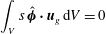
, and conservation of angular momentum (2.33)must be imposed and serve to uniquely determine$$\begin{eqnarray}\displaystyle \int _{V}s\,\hat{\unicode[STIX]{x1D753}}\boldsymbol{\cdot }\boldsymbol{u}_{g}\,\text{d}V=0 & & \displaystyle\end{eqnarray}$$
$u_{g}$
.






The equations developed thus far capture the spirit of our method for the calculation of the sensitivity of
 $\unicode[STIX]{x1D712}^{2}$
with respect to
 $u_{g}$
, allowing the limit
 $\unicode[STIX]{x1D712}^{2}\rightarrow 0$
to be reached. Actual details of implementation differ somewhat, as they depend on the choice of a method for the numerical time stepping of the equations. We discuss these details in appendix E where we give an implementation specific to the Adams–Bashforth time-stepping scheme.
3 Numerical implementation
3.1 Spatial discretization
Our implementation relies on a fully spectral Galerkin method, which is expected to deliver rapid convergence for spatially smooth solutions. We build on the work of Livermore & Ierley (Reference Livermore and Ierley2009), Livermore (Reference Livermore2010) and Li, Jackson & Livermore (Reference Li, Jackson and Livermore2011). For the magnetic and velocity fields we use the classic Mie representation, which ensures that the solenoidality condition is satisfied. Using capital letters to represent quantities associated with the magnetic field and lower case for velocity field, we therefore expand the ageostrophic flow (the ‘magnetic wind’) and the magnetic field,
 $\boldsymbol{u}_{m}$
and
 $\boldsymbol{B}$
, using the poloidal–toroidal decomposition
 $$\begin{eqnarray}\displaystyle \boldsymbol{B}=\boldsymbol{S}+\boldsymbol{T}=\mathop{\sum }_{(n,l,m)}S_{(n,l,m)}\hat{\boldsymbol{S}}_{(n,l,m)}+T_{(n,l,m)}\hat{\boldsymbol{T}}_{(n,l,m)}, & & \displaystyle\end{eqnarray}$$
where
 $$\begin{eqnarray}\displaystyle \hat{\boldsymbol{S}}_{(n,l,m)}=\unicode[STIX]{x1D735}\times \unicode[STIX]{x1D735}\times [\unicode[STIX]{x1D6F7}_{n}^{l}(r)Y_{l}^{m}(\unicode[STIX]{x1D703},\unicode[STIX]{x1D719})\hat{\boldsymbol{r}}],\quad \hat{\boldsymbol{T}}_{(n,l,m)}=\unicode[STIX]{x1D735}\times [\unicode[STIX]{x1D6F9}_{n}^{l}(r)Y_{l}^{m}(\unicode[STIX]{x1D703},\unicode[STIX]{x1D719})\hat{\boldsymbol{r}}]. & & \displaystyle\end{eqnarray}$$
The basis functions have the property
 $$\begin{eqnarray}\displaystyle & \displaystyle \int _{V+\hat{V}}\hat{\boldsymbol{S}}_{(n_{1},l_{1},m_{1})}\boldsymbol{\cdot }\hat{\boldsymbol{S}}_{(n_{2},l_{2},m_{2})}\,\text{d}V=\int _{V}\hat{\boldsymbol{T}}_{(n_{1},l_{1},m_{1})}\boldsymbol{\cdot }\hat{\boldsymbol{T}}_{(n_{2},l_{2},m_{2})}\,\text{d}V=\unicode[STIX]{x1D6FF}_{n_{1},n_{2}}\unicode[STIX]{x1D6FF}_{l_{1},l_{2}}\unicode[STIX]{x1D6FF}_{m_{1},m_{2}}, & \displaystyle\end{eqnarray}$$
 $$\begin{eqnarray}\displaystyle & \displaystyle \int _{V+\hat{V}}\hat{\boldsymbol{S}}_{(n_{1},l_{1},m_{1})}\boldsymbol{\cdot }\hat{\boldsymbol{T}}_{(n_{2},l_{2},m_{2})}\,\text{d}V=0. & \displaystyle\end{eqnarray}$$
In (3.2),
 $Y_{l}^{m}(\unicode[STIX]{x1D703},\unicode[STIX]{x1D719})$
is a fully normalized spherical harmonic of degree
 $l$
and order
 $m$
whose squared integral over the sphere is unity, and
 $S_{(n,l,m)}$
and
 $T_{(n,l,m)}$
are the spectral coefficients for
 $\boldsymbol{B}$
where
 $n$
is a radial index. The Galerkin radial basis functions
 $\unicode[STIX]{x1D6F7}_{n}^{l}$
and
 $\unicode[STIX]{x1D6F9}_{n}^{l}$
are polynomials in which the required boundary conditions are encoded (see appendix D for details). Thus each
 $\hat{\boldsymbol{S}}$
and
 $\hat{\boldsymbol{T}}$
individually satisfies the boundary conditions. These basis functions have been constructed by using the fundamental Jones–Worland polynomials (Livermore, Jones & Worland Reference Livermore, Jones and Worland2007) as building blocks. Such functions have been analysed by Marti & Jackson (Reference Marti and Jackson2016), particularly with respect to their smooth differentiable nature at the origin of the coordinate system. A key feature of the basis when used in a time-stepping scheme is the fact that the Courant–Friedrichs–Lewy condition remains innocuous near the origin (Marti & Jackson Reference Marti and Jackson2016), something that is hard to achieve in other (e.g. finite difference) methods.
Similarly, the ageostrophic flow is represented as
 $$\begin{eqnarray}\displaystyle \boldsymbol{u}_{m}=\mathop{\sum }_{(n,l,m)}s_{(n,l,m)}\hat{\boldsymbol{s}}_{(n,l,m)}+t_{(n,l,m)}\hat{\boldsymbol{t}}_{(n,l,m)}, & & \displaystyle\end{eqnarray}$$
where
 $$\begin{eqnarray}\displaystyle \hat{\boldsymbol{s}}_{(n,l,m)}=\unicode[STIX]{x1D735}\times \unicode[STIX]{x1D735}\times [\unicode[STIX]{x1D6F1}_{n}^{l}(r)Y_{l}^{m}(\unicode[STIX]{x1D703},\unicode[STIX]{x1D719})\hat{\boldsymbol{r}}],\quad \hat{\boldsymbol{t}}_{(n,l,m)}=\unicode[STIX]{x1D735}\times [\unicode[STIX]{x1D6EF}_{n}^{l}(r)Y_{l}^{m}(\unicode[STIX]{x1D703},\unicode[STIX]{x1D719})\hat{\boldsymbol{r}}], & & \displaystyle\end{eqnarray}$$
and the radial Galerkin functions
 $\unicode[STIX]{x1D6F1}_{n}^{l}$
and
 $\unicode[STIX]{x1D6EF}_{n}^{l}$
are suitably defined in order that
 $\hat{\boldsymbol{t}}_{(n,l,m)}$
and
 $\hat{\boldsymbol{s}}_{(n,l,m)}$
satisfy both their boundary conditions and a similar orthonormality relation to (3.4) (see appendix D). It is worth noting that, of the four classes of basis function, only
 $\hat{\boldsymbol{S}}_{(n,l,m)}$
is non-zero in
 $\hat{V}$
.
The remaining geostrophic flow is represented as
 $$\begin{eqnarray}\displaystyle \boldsymbol{u}_{g}=\mathop{\sum }_{k}g_{k}\unicode[STIX]{x1D6EC}_{k}(s)\hat{\unicode[STIX]{x1D753}}, & & \displaystyle\end{eqnarray}$$
with coefficients
 $g_{k}$
, where the basis functions
 $\unicode[STIX]{x1D6EC}_{k}$
(see appendix D) are orthonormal when integrated over the volume of the unit sphere (recall
 $A(s)$
is defined in (2.27)),
 $$\begin{eqnarray}\displaystyle \int _{0}^{1}A(s)\unicode[STIX]{x1D6EC}_{j}(s)\unicode[STIX]{x1D6EC}_{k}(s)\,\text{d}s=\unicode[STIX]{x1D6FF}_{j,k}. & & \displaystyle\end{eqnarray}$$
As will be described in § 3.2, we note that the only component of flow that carries angular momentum is
 $\unicode[STIX]{x1D6EC}_{1}$
.
Because our basis functions
 $\hat{\boldsymbol{S}}$
,
 $\hat{\boldsymbol{T}}$
,
 $\hat{\boldsymbol{s}}$
and
 $\hat{\boldsymbol{t}}$
are defined in terms of spherical harmonics and regular polynomials in radius, they may be equivalently represented in Cartesian coordinates as polynomials. This not only allows us to calculate quantities such as (1.1) exactly, but also permits us to define a largest polynomial degree of the Cartesian components which defines a measure of spatial complexity. By using a triangular truncation for the radial index (Ivers, Jackson & Winch Reference Ivers, Jackson and Winch2015), we adopt a resolution uniform in each coordinate direction (see table 1). At each spherical harmonic degree
 $l$
, the maximum radial index is
 $(L_{max}+q)/2-\lfloor (l-(1-q))/2\rfloor$
with
 $q=L_{max}~\text{mod}\,2$
.
Our fields
 $\boldsymbol{B}$
,
 $\boldsymbol{u}_{m}$
and
 $u_{g}$
are truncated at
 $L_{B}$
,
 $L_{u_{m}}$
and
 $N$
, respectively. We sometimes report a truncation of
 $L_{max}$
, which means
 $L_{B}=L_{max}$
,
 $L_{u_{m}}=2L_{B}$
and
 $N=L_{max}$
, which is the natural band limit for the fields (recall that
 $u_{g}/s$
is an even polynomial so that the largest degree is then
 $2L_{max}-1$
and has the same complexity as
 $\boldsymbol{u}_{m}$
), but some calculations have to resort to more aggressively truncated fields.
We work in the subspace of truncated polynomials for all our fields. Little is known about the behaviour of the geostrophic flow in general, and there are examples of
 $\unicode[STIX]{x1D6FC}$
distributions, albeit non-polynomial ones, for which
 $u_{g}$
exhibits singularities. We have received a demonstration from Professor G. Ierley, who has completed the analysis of Greenspan (Reference Greenspan1974), showing that the geostrophic flow does not necessarily remain finite at
 $s=1$
. This is presented in appendix F.
The maximum radial index
 $N_{max}$
as a function of spherical degree
 $l$
, where
 $L_{max}$
is the maximum degree of the spherical harmonic expansion.

3.2 Algorithm for finding the ageostrophic flow
In the exact magnetostrophic balance (2.6), in which the magnetic field necessarily satisfies Taylor’s constraint, Taylor showed that
 $\boldsymbol{u}_{m}$
is uniquely determined up to the geostrophic flow for a given forcing term
 $\boldsymbol{F}$
(here, the Lorentz force
 $\unicode[STIX]{x1D735}\times \boldsymbol{B}\times \boldsymbol{B}$
). Because of our fully spectral representation of
 $\boldsymbol{B}$
, the forcing term has Cartesian components that are polynomial (of the form
 $x^{a}y^{b}z^{c}$
) and are of some maximum degree
 $P$
. We further observe that if the operator
 $\hat{\boldsymbol{z}}\,\times$
acts upon a vector with polynomial coefficients, it does not alter the maximum degree. Because the pressure term can be eliminated by taking the curl, it follows that the space of solutions for the ageostrophic flow is spanned by those fully spectral basis functions (defined in § 3.1) which have Cartesian components of degree no greater than
 $P$
. We may construct a closed system of equations for the unknown poloidal and toroidal modal coefficients by back-projecting onto the same set of velocity modes of degrees up to
 $P$
; thus we find the spectral flow coefficients as
 $\unicode[STIX]{x1D648}^{-1}\,\boldsymbol{f}$
, where
 $$\begin{eqnarray}\displaystyle \unicode[STIX]{x1D614}_{i,j}=M(\boldsymbol{u}_{i},\boldsymbol{u}_{j})=\int _{V}\boldsymbol{u}_{i}\boldsymbol{\cdot }(\hat{\boldsymbol{z}}\times \boldsymbol{u}_{j})\,\text{d}V,\quad \boldsymbol{f}_{i}=\int _{V}\boldsymbol{u}_{i}\boldsymbol{\cdot }\boldsymbol{F}\,\text{d}V. & & \displaystyle\end{eqnarray}$$
We note that the pressure term vanishes in the above projection procedure by virtue of the divergence theorem, along with exploiting incompressibility and impenetrability of the boundary.
The results we shall present in §§ 6–8 have very small values of
 $\unicode[STIX]{x1D712}^{2}$
(as measured by (1.2)), indicating a close adherence to Taylor’s constraint. However, numerically it is impossible to achieve an exactly zero
 ${\mathcal{T}}$
everywhere in (1.1). It is therefore worth considering the repercussions of this for our algorithm for finding
 $\boldsymbol{u}_{m}$
, in light of the fact that (3.9) was developed assuming an exact magnetostrophic balance. When
 ${\mathcal{T}}\neq 0$
for all
 $s$
, the band-limited property of
 $\boldsymbol{u}_{m}$
alluded to above is lost. However, the matrix
 $\unicode[STIX]{x1D648}$
remains invertible and we can nevertheless continue to solve for
 $\boldsymbol{u}_{m}$
using (3.9), and we do so using the same truncation as before.
To simplify the numerics, we note that the sparse matrix
 $\unicode[STIX]{x1D648}$
separates into azimuthal modes and by equatorial symmetry (see appendix A). The axisymmetric class containing the geostrophic component needs to be treated carefully, as the matrix
 $\unicode[STIX]{x1D648}$
is formally singular in this case. One way of eliminating the geostrophic degeneracy is to remove all lowest-radial-order odd-
 $l$
toroidal modes from the representation. The cylindrical average of the azimuthal component can then be removed from the resulting flow. In all symmetry classes, therefore, this procedure results in the ageostrophic flow with no geostrophic component.
We remark that this construction ensures that the ageostrophic flow carries no angular momentum. To show this we note that to extract the angular momentum from a general flow
 $\boldsymbol{U}$
one needs to take the inner product
 $$\begin{eqnarray}\displaystyle \langle \hat{\boldsymbol{t}}_{(1,1,0)}\boldsymbol{\cdot }\boldsymbol{U}\rangle . & & \displaystyle\end{eqnarray}$$
However, no mode in the ageostrophic flow other than
 $\hat{\boldsymbol{t}}_{(1,1,0)}$
can carry angular momentum. But having removed the geostrophic component from
 $\boldsymbol{u}_{m}$
, one can see that it carries no angular momentum at all. Only the geostrophic component then contributes to the angular momentum:
 $$\begin{eqnarray}\displaystyle \int A(s)su_{g}(s)\,\text{d}s & & \displaystyle\end{eqnarray}$$
and we note that in our basis the polynomial ‘
 $s$
’ appearing in (3.11) is just a scalar multiple of
 $\unicode[STIX]{x1D6EC}_{1}$
, the solid-body component of the flow. Thus we see from (3.8) that all angular momentum is carried by the coefficient
 $g_{1}$
and therefore it must be set to zero. This is not updated by use of the gradient, whilst all other
 $N-1$
components are.
3.3 A smoothness-inducing linear friction model
Computationally we face a cascade to smaller wavenumbers at each time step: suppose that at time
 $t$
the spatial complexity of the magnetic field is
 $L_{max}$
. The magnetostrophic equation (2.6) is quadratic in
 $\boldsymbol{B}$
, which creates a
 $\boldsymbol{u}_{m}$
that is of complexity
 $2L_{max}$
, whilst the induction term,
 $\unicode[STIX]{x1D735}\times (\boldsymbol{u}\times \boldsymbol{B})$
, further increases the spatial complexity of
 $\boldsymbol{B}$
to
 $3L_{max}$
after a time step. Hence at every time step, we have to truncate the magnetic field at
 $L_{max}$
and it is this truncated field that is forced to satisfy Taylor’s condition (i.e. the maximum degree of
 $\boldsymbol{B}$
in (1.1) is
 $L_{max}$
while the degree of (1.2) is twice this). This truncation error is inevitably injected into the computation of
 $\boldsymbol{u}_{g}$
. After a large number of computational time steps, the accumulated truncation error inversely cascades into the spectrum of
 $\boldsymbol{u}_{g}$
and eventually destroys its convergence.
To combat this effect we introduce a linear friction model previously employed by Hollerbach & Ierley (Reference Hollerbach and Ierley1991), drawing on the oceanographic implementation of Salmon (Reference Salmon1986). We shall show the adoption of this idea to be beneficial in suppressing small-scale structures that have little effect on the magnetic field at the time horizon, and that the linear friction will always be below the level of the Lorentz torque
 ${\mathcal{T}}$
. We define a damping term as
 ${\mathcal{L}}=-\{\boldsymbol{u}_{g}\}$
(noting that the geostrophic flow vanishes outside of
 $V$
), which together with a pseudo-Ekman number
 $\unicode[STIX]{x1D716}^{2}$
satisfies
 $$\begin{eqnarray}\displaystyle \unicode[STIX]{x1D716}\Vert {\mathcal{L}}(\boldsymbol{u}_{g})\Vert \ll \Vert {\mathcal{T}}\Vert \ll 1. & & \displaystyle\end{eqnarray}$$
Correspondingly, in our numerical model, Taylor’s integral
 ${\mathcal{T}}$
is replaced by
 ${\mathcal{T}}-\unicode[STIX]{x1D716}\{\boldsymbol{u}_{g}\}$
and a suitably modified version of
 $\unicode[STIX]{x1D712}^{2}$
is used. We note that there is a link between this approach and that of an Ekman state formulation, in which boundary friction is used to balance Taylor torques. The correspondence is not exact, as we omit the geometric factor containing a singularity at
 $s=1$
, but
 $\unicode[STIX]{x1D716}$
can be seen to be akin to
 $\sqrt{E}$
. This friction term appears in our objective function but none of the underlying physical equations are altered. Thus we still seek purely magnetostrophic states (that is, with zero viscosity); the introduction of the pseudo-Ekman number merely assists us in finding them numerically. In appendix E, we derive the discretized version of the continuous model (E 3) presented in § 2 using this modified version of the target function.
3.4 On the choice of weight function
$w$

The choice of the positive weight function
 $w(s)$
has thus far remained arbitrary. We will report calculations with
 $w(s)=(1-s^{2})^{\unicode[STIX]{x1D6FE}}$
with three choices of
 $\unicode[STIX]{x1D6FE}$
, namely
 $(-1/2,0,1/2)$
. We will show in subsequent examples that the choice of
 $\unicode[STIX]{x1D6FE}$
has very little effect on the solutions obtained.
There is a need to compute a number of integrals in cylindrical coordinates, such as the value of the Taylor torque (1.1) and its downhill direction (2.32). With our polynomial basis for
 $\boldsymbol{B}$
and
 $\boldsymbol{B}^{\dagger }$
, all of these integrals can be computed exactly by using quadrature rules appropriate for the weighting function chosen. For example,
 $w=1$
dictates that we use Gauss–Legendre quadrature, and
 $w=(1-s^{2})^{-1/2}$
dictates that we use Gauss–Chebyshev quadrature.
3.5 The use of gradients in the update of
$\boldsymbol{u}_{g}$

Note that the target
 $\unicode[STIX]{x1D712}^{2}$
as defined in (1.2) is a quartic functional with respect to
 $\boldsymbol{B}$
that can tend to zero as a result of both adherence to Taylor’s constraint, or if
 $\boldsymbol{B}\rightarrow 0$
. We define a normalized quantity
 $\mathbb{T}$
, here dubbed the ‘Taylicity’ (we coin the term ‘Taylicity’ to avoid confusion with the term ‘Taylorization’ (Rotvig & Jones Reference Rotvig and Jones2002), which has a different definition and is not a differentiable function of the magnetic field) to quantify the adherence to Taylor’s constraint:
 $$\begin{eqnarray}\displaystyle \mathbb{T}=\frac{\unicode[STIX]{x1D712}^{2}}{\langle \boldsymbol{B}^{2}\rangle ^{2}}. & & \displaystyle\end{eqnarray}$$
We seek the optimal solution for
 $\boldsymbol{u}_{g}$
by minimizing the misfit,
 $\unicode[STIX]{x1D712}^{2}$
, using the following procedure:
(i) At
$t=0$
, we start with a
$\boldsymbol{B}$
field in a Taylor state, calculate
$\boldsymbol{u}_{m}$
(assumed constant for
$t\in [0,\unicode[STIX]{x0394}t]$
) by (3.9) and take
$\boldsymbol{u}_{g}=0$
; we then forward evolve (2.7) from
$t=0$
to
$t=\unicode[STIX]{x0394}t$
.(ii) We compute the Taylicity,
$\mathbb{T}$
, defined in (3.13).(iii) We compute the downhill direction,
$-\unicode[STIX]{x1D735}_{\boldsymbol{u}_{g}}\unicode[STIX]{x1D712}^{2}$
, with respect to
$\boldsymbol{u}_{g}$
using the adjoint method.(iv) We use the limited memory L-BFGS algorithm (Nocedal & Wright Reference Nocedal and Wright2006), a gradient-based optimization method, to calculate an updated
$\boldsymbol{u}_{g}$
: (3.14)where$$\begin{eqnarray}\displaystyle \boldsymbol{u}_{g}^{(i+1)}=\boldsymbol{u}_{g}^{(i)}-\unicode[STIX]{x1D70C}{\mathcal{H}}^{-1}\unicode[STIX]{x1D735}_{\boldsymbol{u}_{g}}\unicode[STIX]{x1D712}^{2}, & & \displaystyle\end{eqnarray}$$
$\boldsymbol{u}_{g}^{(i)}$
is the solution of the geostrophic flow at the
$i$
th iteration,
${\mathcal{H}}^{-1}$
is the estimate of the inverse Hessian built up by BFGS and based on previous iterations, and
$\unicode[STIX]{x1D70C}$
is the step length (Nocedal Reference Nocedal1980). Angular momentum conservation is respected as described in § 3.2.(v) We keep iterating (ii)–(iv) until the normalized misfit is less than or equal to a target or threshold value,
$\unicode[STIX]{x1D712}_{T}^{2}$
, i.e.,
$\mathbb{T}\leqslant \unicode[STIX]{x1D712}_{T}^{2}$
.(vi) When condition (v) is satisfied, the solution of
$\boldsymbol{B}$
,
$\boldsymbol{u}_{m}$
and
$\boldsymbol{u}_{g}$
at
$t=\unicode[STIX]{x0394}t$
is accepted as the optimal Taylor state solution and we move on to the next time step.





4 Two algorithm benchmarks using a single time step,
$\unicode[STIX]{x0394}t$

In this section we report two different tests to demonstrate that we can successfully determine the geostrophic flow using our algorithms. The first compares two numerical schemes for recovering
 $u_{g}$
over an arbitrary time step
 $\unicode[STIX]{x0394}t$
. The comparison is between a so-called ‘brute-force’ technique for determining the derivative of
 $\unicode[STIX]{x1D712}^{2}$
with respect to
 $u_{g}$
, which is straightforward and simple (thus reducing the likelihood of analytic or coding errors), but which requires
 $N$
times more evaluations than our adjoint method; in our tests we use a resolution
 $N=30$
. The second check compares an instantaneous solution for
 $u_{g}$
, which can be determined analytically for a very special choice of initial condition for
 $\boldsymbol{B}$
, with that determined by our scheme. When
 $\unicode[STIX]{x0394}t$
is chosen to be small, the two should agree, as indeed they do. In the following sections we set
 $\unicode[STIX]{x1D716}=0$
(see § 3.3) and
 ${\mathcal{E}}=0$
(2.8).
4.1 Numerical verification of the gradient computation
In order to demonstrate the veracity of the derivations and their numerical implementation, we undertake a comparison of our gradient calculation against the so-called ‘brute-force’ method. We test using the most general structure of the initial magnetic field, which is not a Taylor state, shown in (figure 1
a). We also use an arbitrary ageostrophic flow and geostrophic flow,
 $\boldsymbol{u}_{g}$
(figure 1
b); this assignment means that (2.6) is not obeyed in this test. No aspect of this brute-force test relies on the adherence to a magnetostrophic balance.
(a) The poloidal and (b) toroidal components of the axisymmetric initial magnetic field used in the gradient benchmark: (a) the stream function is shown, such that field lines are parallel to contours, and (b) the
 $\unicode[STIX]{x1D719}$
component of the field is shown. (c) The initial geostrophic flow,
 $\boldsymbol{u}_{g}$
, and (d) Taylor’s integral,
 ${\mathcal{T}}$
, of the prescribed
 $\boldsymbol{B}$
as functions of
 $s$
.

We forward evolve (2.7) and (2.30)–(2.31) for one time step
 $\unicode[STIX]{x0394}t=10^{-6}$
, and compute the gradient,
 $\unicode[STIX]{x1D735}_{\boldsymbol{u}_{g}}\unicode[STIX]{x1D712}^{2}$
, via
(i) the adjoint method (2.32) and
(ii) a brute-force method in which we perturb each coefficient,
$g_{k}$
, of
$\boldsymbol{u}_{g}$
, in sequence with
$\unicode[STIX]{x1D6FF}g_{k}/g_{k}=10^{-3}$
, and compute the
$k$
th entry of the gradient in terms of
$\unicode[STIX]{x0394}\unicode[STIX]{x1D712}_{k}^{2}/\unicode[STIX]{x1D6FF}g_{k}$
.


Figure 2 illustrates the gradient comparison for this scenario, comparing
 $\unicode[STIX]{x1D735}_{\boldsymbol{u}_{g}}\unicode[STIX]{x1D712}^{2}$
of the adjoint method and the brute-force method for each of the spectral coefficients of
 $\boldsymbol{u}_{g}$
using different weight functions,
 $w$
. We set the spatial resolution as
 $L_{B}=30$
,
 $L_{u_{m}}=60$
and
 $N_{u_{g}}=30$
. The adjoint method is seen to be accurate for all weight functions.
Comparison of the gradient computations,
 $\unicode[STIX]{x1D735}_{\boldsymbol{u}_{g}}\unicode[STIX]{x1D712}^{2}$
, using the adjoint method (green dots) and brute-force method (red open squares) for different weight functions
 $w=(1-s^{2})^{\unicode[STIX]{x1D6FE}}$
for (a)
 $\unicode[STIX]{x1D6FE}=0$
, (b)
 $\unicode[STIX]{x1D6FE}=-1/2$
and (c)
 $\unicode[STIX]{x1D6FE}=1/2$
. In all cases, the green and red symbols overplot. The ordinate shows the index of the spectral coefficient
 $g_{n}$
of
 $\boldsymbol{u}_{g}$
. The time step taken is
 $\unicode[STIX]{x0394}t=10^{-6}$
, and truncation levels are
 $L_{B}=30$
,
 $L_{u_{m}}=60$
and
 $N_{u_{g}}=30$
.

4.2 Benchmark against a Taylor-type analytic solution for
$\boldsymbol{u}_{g}$

A second comparison can be made between our methodology and that of Taylor when
 $\unicode[STIX]{x0394}t$
is small. We look for an instantaneous solution for
 $\boldsymbol{u}_{m}$
and
 $\boldsymbol{u}_{g}$
when the field
 $\boldsymbol{B}$
is prescribed, where
 $$\begin{eqnarray}\displaystyle \boldsymbol{B}=16\sqrt{\frac{7\unicode[STIX]{x03C0}}{3}}\hat{\boldsymbol{S}}_{(1,2,0)}=\left\{\begin{array}{@{}ll@{}}\unicode[STIX]{x1D735}\times \unicode[STIX]{x1D735}\times [r^{3}(5r^{2}-7)(3\cos ^{2}\unicode[STIX]{x1D703}-1)\hat{\boldsymbol{r}}], & r\in [0,1],\\ -2\unicode[STIX]{x1D735}r^{-3}(3\cos ^{2}\unicode[STIX]{x1D703}-1), & r\in [1,\infty ).\end{array}\right. & & \displaystyle\end{eqnarray}$$
Such a single-mode choice for
 $\boldsymbol{B}$
is automatically a Taylor state (Livermore, Ierley & Jackson Reference Livermore, Ierley and Jackson2008, Reference Livermore, Ierley and Jackson2009). For this choice of
 $\boldsymbol{B}$
, the velocity fields
 $\boldsymbol{u}_{m}$
and
 $\boldsymbol{u}_{g}$
have closed analytic forms. We solve the magnetostrophic equation (2.6) to obtain
 $\boldsymbol{u}_{m}$
. To obtain
 $u_{g}$
, we differentiate (1.3) with respect to time and demand that
 $\unicode[STIX]{x2202}{\mathcal{T}}/\unicode[STIX]{x2202}t=0$
. This leads to a first-order differential equation (Wu & Roberts Reference Wu and Roberts2015) for
 $d_{s}(u_{g}/s)$
, where
 $d_{s}=\text{d}/\text{d}s$
, that has an analytical solution in this case. Note that in the presence of viscosity
 $\unicode[STIX]{x1D708}$
, the term
 $\unicode[STIX]{x1D708}sd_{s}(u_{g}/s)$
would be the stress of the geostrophic flow in the tangential direction of the geostrophic cylinder. We make use of this in our diagnostics.
For our chosen single mode
 $\boldsymbol{B}$
, the instantaneous solution for
 $\boldsymbol{u}_{m}$
is
 $$\begin{eqnarray}\displaystyle \boldsymbol{u}_{m}=210r\sin (\unicode[STIX]{x1D703})[22-70r^{2}+39r^{4}-2(r^{2}+7)r^{2}\cos (2\unicode[STIX]{x1D703})-7r^{4}\cos (4\unicode[STIX]{x1D703})]\hat{\unicode[STIX]{x1D753}}, & & \displaystyle\end{eqnarray}$$
and the geostrophic flow has a closed-form solution,
 $$\begin{eqnarray}\displaystyle u_{g} & = & \displaystyle {\textstyle \frac{5}{4}}s\{\!48(81s^{2}+62)s^{2}-688\log (5(s^{2}-2)s^{2}+6)\nonumber\\ \displaystyle & & \displaystyle -\,2464\sqrt{5}\tan ^{-1}(\sqrt{5}(s^{2}-1))-896\log (s)+4557\!\}+\,c_{1}s.\end{eqnarray}$$
The constant
 $c_{1}\approx -14282.627018357707$
is the strength of the solid-body rotation component and is chosen so that the angular momentum of the flow in the
 $\hat{\unicode[STIX]{x1D753}}$
direction remains zero. Within our axisymmetric system, we note that the form of the geostrophic flow contains an
 $s\log s$
term, which means that the flow is not differentiable at
 $s=0$
(e.g. Fearn & Proctor Reference Fearn and Proctor1987; Jault Reference Jault1995; Wu & Roberts Reference Wu and Roberts2015). We have chosen not to make any special accommodation for this term, remaining instead with our polynomial description of
 $u_{g}$
. The polynomial description can, of course, adequately synthesize most continuous functions, as we shall see, although it does not capture the singular derivatives, being itself everywhere regular.
We compare Taylor’s solution to the results of our own method with time step
 $\unicode[STIX]{x0394}t=10^{-6}$
and spatial and temporal resolutions
 $L_{B}=30$
,
 $L_{u_{m}}=60$
and
 $L_{u_{g}}=30$
. We determine
 $\boldsymbol{u}_{m}$
using our matrix solver and, in this special case, the solution for
 $\boldsymbol{u}_{m}$
is entirely toroidal; we find the analytic and the numerical solutions for
 $\boldsymbol{u}_{m}$
are identical up to machine precision. We initially set the geostrophic flow,
 $\boldsymbol{u}_{g}$
, to zero as our starting value and forward evolve the induction equation from
 $t=0$
to
 $t=\unicode[STIX]{x0394}t$
and obtain a normalized misfit (Taylicity),
 $\unicode[STIX]{x1D712}_{0}^{2}$
, as a reference value. We perform a number of iterations to gradually refine our estimate of
 $u_{g}$
. The optimization stops when
 $\mathbb{T}\leqslant \unicode[STIX]{x1D712}_{T}^{2}$
is satisfied. We use a reduction factor,
 $R_{d}$
, to quantify the stringentness of the optimization, setting the threshold to be
 $\unicode[STIX]{x1D712}_{T}^{2}=R_{d}\unicode[STIX]{x1D712}_{0}^{2}$
. Figure 3 compares the numerical and analytic solutions for different weight functions,
 $w$
, and reduction factors,
 $R_{d}$
. An accurate solution is obtained if
 $\unicode[STIX]{x1D712}_{T}^{2}$
is made sufficiently small. For the case
 $R_{d}=10^{-6}$
, the numerical and the analytic solutions are identical, except for a very small deviation of
 $\boldsymbol{u}_{g}$
at
 $s=0$
, due to the
 $s\log s$
singularity. The three different weight functions,
 $w$
, appear to perform equally well. As noted in § 3.4, we prefer to use
 $w=(1-s^{2})^{-1/2}$
as a weight function in order to cancel the geometric factor
 $\sqrt{1-s^{2}}$
, rendering all important quantities polynomial (e.g.
 $\boldsymbol{B}_{\unicode[STIX]{x0394}t}^{\dagger }$
, see (E 5)) and adopt this for all subsequent calculations.
Plots of
 $u_{g}$
and
 $d_{s}(u_{g}/s)$
as a function of
 $s$
comparing the numerical and analytic instantaneous solution (4.3) for the single-mode assignment of
 $\boldsymbol{B}$
given in (4.1). (a–e) The numerical solution (in dashed green) versus the analytic solutions (in red) with different weight functions,
 $w$
, and reduction factors,
 $R_{d}$
. (f) Plot of
 $d_{s}(u_{g}/s)$
as a function of
 $s$
, where the red curve is the analytic solution and the green, blue, orange and purple ones (these latter three curves almost entirely overlaying one another) correspond to the numerical solutions of
 $\boldsymbol{u}_{g}$
in (a–d), respectively. Only in such a derivative plot does the
 $s\log s$
singularity show itself markedly.

5 Axisymmetric examples of dynamo models: kinematics
The preceding description of our modelling strategy in §§ 2 and 3 is inherently 3D. However, in order to simplify the calculations and also to benchmark against other results obtained using independent methods, in the rest of the paper we specialize our analysis to purely axisymmetric examples. In this section we set out the mathematical models that we wish to pursue for the rest of the paper. We begin by deriving kinematic results that verify our numerical methods, before enlarging the discussion to encompass the dynamical constraints from magnetostrophic equilibrium in §§ 6–8.
As is well known, axisymmetric systems cannot sustain a magnetic field without mean-field effects (Cowling Reference Cowling1933); of particular note are the two end-member and widely studied
 $\unicode[STIX]{x1D6FC}^{2}$
and
 $\unicode[STIX]{x1D6FC}{-}\unicode[STIX]{x1D714}$
models (Steenbeck, Krause & Rädler Reference Steenbeck, Krause and Rädler1966). In the so-called
 $\unicode[STIX]{x1D6FC}^{2}$
dynamo model, the generation of both the poloidal and the toroidal fields are due to helical motion parametrized by the given
 $\unicode[STIX]{x1D6FC}$
. In contrast, in an
 $\unicode[STIX]{x1D6FC}{-}\unicode[STIX]{x1D714}$
model, twisting helical flow creates poloidal field from the toroidal magnetic field, whereas toroidal magnetic field is created from the poloidal field due to the flow’s differential rotation, parametrized by
 $\unicode[STIX]{x1D714}$
; such models are typically oscillatory.
A description of the
 $\unicode[STIX]{x1D6FC}$
-effect is the most straightforward of the two models. A turbulent EMF
 ${\mathcal{E}}$
is supposed to be created by small-scale motions, and is a prescribed input to the model of the form
 $$\begin{eqnarray}\displaystyle {\mathcal{E}}=\unicode[STIX]{x1D6FC}\boldsymbol{B}. & & \displaystyle\end{eqnarray}$$
In addition we use
 $\unicode[STIX]{x1D6FC}{-}\unicode[STIX]{x1D714}$
models (5.9), which are more complex and are described in Roberts (Reference Roberts1972) and Wu & Roberts (Reference Wu and Roberts2015). In these models a prescribed shear is added to the ageostrophic flow governed by (2.6). However, certain terms associated with the
 $\unicode[STIX]{x1D6FC}$
-effect are omitted from the equation governing the creation of the toroidal field, the argument being that the
 $\unicode[STIX]{x1D714}$
-effect is much greater than these terms.
For our
 $\unicode[STIX]{x1D6FC}$
-effect models we use two different prescriptions of
 $\unicode[STIX]{x1D6FC}$
: we use the original Braginsky
 $\unicode[STIX]{x1D6FC}$
term,
 $\unicode[STIX]{x1D6FC}_{B}$
(Roberts Reference Roberts1972), and a newly created
 $\unicode[STIX]{x1D6FC}$
term,
 $\unicode[STIX]{x1D6FC}_{L}$
, as the source terms of the
 $\unicode[STIX]{x1D6FC}$
-effects, where
 $$\begin{eqnarray}\displaystyle \unicode[STIX]{x1D6FC}_{B}=\frac{729}{16}r^{8}(1-r^{2})^{2}\cos \unicode[STIX]{x1D703} & & \displaystyle\end{eqnarray}$$
and
 $$\begin{eqnarray}\displaystyle \unicode[STIX]{x1D6FC}_{L}=\sqrt{\frac{7}{3}}\frac{343}{48}r^{3}(1-r^{2})^{2}\cos 3\unicode[STIX]{x1D703}. & & \displaystyle\end{eqnarray}$$
We choose
 $\unicode[STIX]{x1D6FC}_{B}$
for comparison with the known results of Wu & Roberts (Reference Wu and Roberts2015) and
 $\unicode[STIX]{x1D6FC}_{L}$
in order to increase the spatial complexity of the solution. Both
 $\unicode[STIX]{x1D6FC}$
terms are antisymmetric (dipole symmetry class) and normalized by their maximum value,
 $\max |\unicode[STIX]{x1D6FC}_{B}|=\max |\unicode[STIX]{x1D6FC}_{L}|=1$
.
The
 $\unicode[STIX]{x1D714}$
term we use is that of Braginsky as described in Roberts (Reference Roberts1972) and Wu & Roberts (Reference Wu and Roberts2015):
 $$\begin{eqnarray}\displaystyle \unicode[STIX]{x1D714}_{B}=-\frac{19\,683}{40\,960}(1-r^{2})^{5}, & & \displaystyle\end{eqnarray}$$
symmetric about the equator (quadrupole symmetry class) and normalized by its largest shear,
 $\max |\unicode[STIX]{x1D735}\unicode[STIX]{x1D714}_{B}|=1$
. The mean-field
 $\unicode[STIX]{x1D6FC}$
and
 $\unicode[STIX]{x1D714}$
terms preserve the symmetry class of the solution of the magnetic field in the induction equation, i.e., for the initial
 $\boldsymbol{B}$
in a dipole/quadrupole (Dp/Qp) symmetric class, the solution of
 $\boldsymbol{B}$
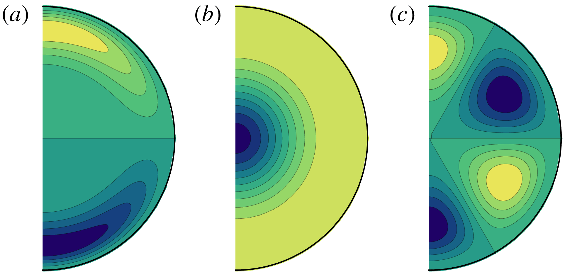
in the induction equation remains in the same class. Figure 4 shows the contours of the mean-field effects.


We are now in a position to compute the kinematic growth rates for the
 $\unicode[STIX]{x1D6FC}$
-effect dynamos by introducing a forcing parameter
 $\unicode[STIX]{x1D6FC}_{0}$
, so that the EMF is
 $$\begin{eqnarray}\displaystyle {\mathcal{E}}=\unicode[STIX]{x1D6FC}_{0}\unicode[STIX]{x1D6FC}\boldsymbol{B}. & & \displaystyle\end{eqnarray}$$
The induction equation being linear in
 $\boldsymbol{B}$
, it is well known that the solutions take the form of eigenmodes
 $\boldsymbol{B}_{i}$
with time dependence
 $$\begin{eqnarray}\displaystyle \boldsymbol{B}_{i}\propto \exp (\unicode[STIX]{x1D706}_{i}t), & & \displaystyle\end{eqnarray}$$
where the eigenvalue
 $\unicode[STIX]{x1D706}_{i}$
can be real or complex. At large times the eigenmode associated with the eigenvalue with largest real part is the one that dominates, and, depending on the degree of forcing, one can find an eigenvalue whose real part is zero. This value of the forcing then defines criticality, or the ability for the field to be sustained against Ohmic decay. Figure 5(a,b) illustrates the eigenvalues of the kinematic
 $\unicode[STIX]{x1D6FC}^{2}$
dynamo,
 $$\begin{eqnarray}\displaystyle \frac{\unicode[STIX]{x2202}\boldsymbol{B}}{\unicode[STIX]{x2202}t}=\unicode[STIX]{x1D6FC}_{0}\unicode[STIX]{x1D735}\times [\unicode[STIX]{x1D6FC}\boldsymbol{B}]+\unicode[STIX]{x1D6FB}^{2}\boldsymbol{B}, & & \displaystyle\end{eqnarray}$$
for
 $\unicode[STIX]{x1D6FC}_{B}$
and
 $\unicode[STIX]{x1D6FC}_{L}$
in Dp and Qp symmetries. Within the range
 $\unicode[STIX]{x1D6FC}_{0}\in [0,20]$
for both
 $\unicode[STIX]{x1D6FC}_{B}$
and
 $\unicode[STIX]{x1D6FC}_{L}$
in Dp and Qp symmetries, the eigenvalues of the leading order of all cases are real, replicating previous results (Roberts Reference Roberts1972). Below the kinematic onset, the magnitude of the decay rate of the dipole field is smaller than that of the quadrupole field. For both
 $\unicode[STIX]{x1D6FC}_{B}$
and
 $\unicode[STIX]{x1D6FC}_{L}$
, the kinematic onset of the dipole and quadrupole fields occur at approximately the same
 $\unicode[STIX]{x1D6FC}_{0}$
(13.1 and 12.5, respectively). For each
 $\unicode[STIX]{x1D6FC}$
term, above the critical
 $\unicode[STIX]{x1D6FC}_{0}$
, the growth rates of the kinematic dynamo for both symmetry classes are nearly identical.
(a,b) The largest eigenvalue of the
 $\unicode[STIX]{x1D6FC}_{B}^{2}$
and
 $\unicode[STIX]{x1D6FC}_{L}^{2}$
dynamos in dipole (green) and quadrupole (red) symmetry. (c) The time evolution of the
 $\unicode[STIX]{x1D6FC}\unicode[STIX]{x1D714}$
kinematic dynamo in terms of
 $\langle \boldsymbol{B}^{2}\rangle /2$
as a function of magnetic decay time, where the solid green, red and blue curves are for
 $\unicode[STIX]{x1D6FC}=-\unicode[STIX]{x1D714}_{0}=200$
, 206 and 210 in the dipole symmetry and the dotted green, red and blue are for
 $\unicode[STIX]{x1D6FC}_{0}=-\unicode[STIX]{x1D714}_{0}=250$
, 254 and 260 in the quadrupole symmetry.

The eigenfunctions
 $\boldsymbol{B}$
when
 $\unicode[STIX]{x1D6FC}_{0}=14$
and
 $\unicode[STIX]{x1D6FC}_{0}=15$
for the
 $\unicode[STIX]{x1D6FC}_{B}^{2}$
and
 $\unicode[STIX]{x1D6FC}_{L}^{2}$
dynamos in both symmetry classes are shown in figure 6, where all magnetic eigenfunctions are normalized so that
 $\langle \boldsymbol{B}^{2}\rangle =1$
. For vector fields such as
 $\boldsymbol{u}$
and
 $\boldsymbol{B}$
we plot the field lines
 $\boldsymbol{B}_{FL}$
and streamlines
 $\boldsymbol{u}_{SF}$
, respectively, in the meridional direction, where their streamfunctions are defined respectively by
 $$\begin{eqnarray}\displaystyle -\sin \,\unicode[STIX]{x1D703}\frac{\unicode[STIX]{x2202}S}{\unicode[STIX]{x2202}\unicode[STIX]{x1D703}}\quad \text{and}\quad -\sin \,\unicode[STIX]{x1D703}\frac{\unicode[STIX]{x2202}s}{\unicode[STIX]{x2202}\unicode[STIX]{x1D703}}, & & \displaystyle\end{eqnarray}$$
and
 $S$
and
 $s$
are the poloidal scalars for the magnetic field and flow. The latter streamlines of course circulate around a suitably modulated streamfunction, hence the moniker
 $\boldsymbol{u}_{SF}$
. The magnetic field lines are concentrated in the region of the strong
 $\unicode[STIX]{x1D6FC}$
-effect.
Contour plots of the linear
 $\unicode[STIX]{x1D6FC}_{B}^{2}$
and
 $\unicode[STIX]{x1D6FC}_{L}^{2}$
kinematic dynamos in dipole and quadrupole symmetry, where
 $\langle \boldsymbol{B}^{2}\rangle =1$
: (a) kinematic
 $\unicode[STIX]{x1D6FC}_{B}^{2}$
dynamo for
 $\unicode[STIX]{x1D6FC}_{0}=14$
in Dp (two leftmost) and Qp (two rightmost) symmetry; (b) kinematic
 $\unicode[STIX]{x1D6FC}_{L}^{2}$
dynamo for
 $\unicode[STIX]{x1D6FC}_{0}=15$
in Dp (two leftmost) and Qp (two rightmost) symmetry. For each dynamo we show the field lines (using (5.8)) and the toroidal field
 $B_{\unicode[STIX]{x1D719}}$
.

We have also studied the following Braginsky
 $\unicode[STIX]{x1D6FC}\unicode[STIX]{x1D714}$
kinematic dynamo for comparison with the results of Wu & Roberts (Reference Wu and Roberts2015); the system evolves according to
 $$\begin{eqnarray}\displaystyle \frac{\unicode[STIX]{x2202}\boldsymbol{B}}{\unicode[STIX]{x2202}t}=\unicode[STIX]{x1D735}\times [\unicode[STIX]{x1D6FC}_{0}\unicode[STIX]{x1D6FC}_{B}\boldsymbol{T}+\unicode[STIX]{x1D714}_{0}(r\sin \unicode[STIX]{x1D703}\,\unicode[STIX]{x1D714}_{B}\hat{\unicode[STIX]{x1D753}})\times \boldsymbol{S}]+\unicode[STIX]{x1D6FB}^{2}\boldsymbol{B}, & & \displaystyle\end{eqnarray}$$
where
 $\boldsymbol{S}$
and
 $\boldsymbol{T}$
are the poloidal and toroidal components of
 $\boldsymbol{B}$
, and
 $\unicode[STIX]{x1D714}_{B}$
is given in (5.4). Unlike the
 $\unicode[STIX]{x1D6FC}^{2}$
kinematic dynamo system, the kinematic dynamo of
 $\unicode[STIX]{x1D6FC}\unicode[STIX]{x1D714}$
type often possesses travelling-wave solutions. This is due to the communication and competition between the
 $\unicode[STIX]{x1D6FC}$
-effect and the
 $\unicode[STIX]{x1D714}$
-effect in different regions within the core. A strong poloidal field results in a strong
 $\unicode[STIX]{x1D714}$
-effect, which converts the poloidal magnetic field into toroidal and weakens the poloidal field itself; simultaneously, a strong toroidal field results in a strong
 $\unicode[STIX]{x1D6FC}$
-effect, which converts the toroidal field into poloidal. As a result, the
 $\unicode[STIX]{x1D6FC}\unicode[STIX]{x1D714}$
kinematic dynamo is usually oscillatory and is measured by the dynamo number,
 ${\mathcal{D}}=\unicode[STIX]{x1D6FC}_{0}\unicode[STIX]{x1D714}_{0}$
, where
 $\unicode[STIX]{x1D6FC}_{0}$
and
 $\unicode[STIX]{x1D714}_{0}$
are the strength of the
 $\unicode[STIX]{x1D6FC}$
- and
 $\unicode[STIX]{x1D714}$
-effect. Figure 5(c) shows the energy of the kinematic
 $\unicode[STIX]{x1D6FC}_{B}\unicode[STIX]{x1D714}_{B}$
dynamo for different dynamo numbers given by
 $\unicode[STIX]{x1D6FC}_{0}=-\unicode[STIX]{x1D714}_{0}$
, in Dp and Qp symmetries. The kinematic onset for the dipole symmetry is approximately
 $\unicode[STIX]{x1D6FC}_{c}=-\unicode[STIX]{x1D714}_{c}=206$
; while the critical value for the quadrupole symmetry is
 $\unicode[STIX]{x1D6FC}_{c}=-\unicode[STIX]{x1D714}_{c}=254$
. The dynamos oscillate rapidly in time; for the dipole field, the oscillation period is approximately 6 % of the magnetic decay time, and for the quadrupole field, it is approximately 5 % of the magnetic decay time (Roberts Reference Roberts1972). Figure 7 illustrates the eigenstates of
 $\boldsymbol{B}$
of the
 $\unicode[STIX]{x1D6FC}_{B}\unicode[STIX]{x1D714}_{B}$
dynamo at the minimal and maximal energy states in dipole and quadrupole symmetries at the kinematic onset values
 $\unicode[STIX]{x1D6FC}_{c}$
and
 $\unicode[STIX]{x1D714}_{c}$
; for the calculations we used resolutions
 $L_{B}=30$
and
 $\unicode[STIX]{x0394}t=10^{-5}$
.
Contour plots and field lines of the
 $\unicode[STIX]{x1D6FC}_{B}\unicode[STIX]{x1D714}_{B}$
kinematic dynamo in dipole and quadrupole symmetry: (a) kinematic
 $\unicode[STIX]{x1D6FC}_{B}\unicode[STIX]{x1D714}_{B}$
dynamo for
 $\unicode[STIX]{x1D6FC}_{0}=-\unicode[STIX]{x1D714}_{0}=206$
in Dp symmetry of the minimum (two leftmost), at
 $t=0.42$
, and the maximum (two rightmost), at
 $t=0.45$
, energy states; (b) kinematic
 $\unicode[STIX]{x1D6FC}_{B}\unicode[STIX]{x1D714}_{B}$
dynamo for
 $\unicode[STIX]{x1D6FC}_{0}=-\unicode[STIX]{x1D714}_{0}=254$
in Qp symmetry of the minimum (two leftmost), at
 $t=0.41$
, and the maximum (two rightmost), at
 $t=0.43$
, energy states.

6 The Braginsky
$\unicode[STIX]{x1D6FC}_{B}$
model and Taylor’s constraint

6.1 The torsional wave (TW) versus the Taylor state (TS) dynamo model
We now extend our investigations to take into account some dynamics. We compare models in which Taylor’s constraint is adhered to (termed TS models) with models that allow for deviations from this state and consequently generate torsional oscillations or waves (termed TW models), as presaged in § 5 of Taylor (Reference Taylor1963) and rigorously studied by Braginsky (Reference Braginsky1970). Such an approach was first implemented by Jault (Reference Jault1995), although much of our discussion builds upon the study of Roberts & Wu (Reference Roberts and Wu2014), who set out the theoretical links between TS (what they term ordinary Taylor theory, OTT) and TW (what they term MTT, modified Taylor theory).
Our model is the following, in which the inertial force is assumed to be negligible except for the geostrophic component, i.e.
 $$\begin{eqnarray}\displaystyle \left.\begin{array}{@{}c@{}}\displaystyle R_{o}\frac{\unicode[STIX]{x2202}\boldsymbol{u}_{g}}{\unicode[STIX]{x2202}t}+\hat{\boldsymbol{z}}\times \boldsymbol{u}_{m}=(\unicode[STIX]{x1D735}\times \boldsymbol{B})\times \boldsymbol{B}-\unicode[STIX]{x1D735}\unicode[STIX]{x1D70B},\\ \displaystyle \frac{\unicode[STIX]{x2202}\boldsymbol{B}}{\unicode[STIX]{x2202}t}=\unicode[STIX]{x1D735}\times [\boldsymbol{u}\times \boldsymbol{B}+{\mathcal{E}}]+\unicode[STIX]{x1D6FB}^{2}\boldsymbol{B},\end{array}\right\} & & \displaystyle\end{eqnarray}$$
where
 ${\mathcal{E}}$
is defined in (5.5),
 $\boldsymbol{u}=\boldsymbol{u}_{m}+\boldsymbol{u}_{g}$
and
 $R_{o}$
is the magnetic Rossby number defined in (2.5). We use the
 $\unicode[STIX]{x1D6FC}_{B}$
-effect in these calculations. The TS model is, of course, defined by
 $R_{o}=0$
, in which case
 $\boldsymbol{u}_{g}$
is determined by the methods of § 2.2, whereas for
 $R_{o}\neq 0$
,
 $\boldsymbol{u}_{g}$
is explicitly deterministic. We envisage that (6.1) evolves towards an equilibrium state, in which the torsional wave stops and the magnetic field becomes stationary in time. Note that
 $\unicode[STIX]{x2202}_{t}u_{g}=0$
is true if and only if Taylor’s condition is satisfied,
 ${\mathcal{T}}=0$
for all
 $s$
. Therefore, at the equilibrium state, the solutions of the TS and TW models are expected to be identical. It is worth noting, however, that, if the torsional wave speed (Roberts & King Reference Roberts and King2013) is locally relatively small at
 $s=s_{a}$
, convergence of the TW model as
 $t\rightarrow \infty$
to the TS model may be slow in the neighbourhood of
 $s_{a}$
. However, the pointwise vanishing of the Alfvén speed is not, in itself, sufficient to prevent the propagation of torsional waves (Maffei & Jackson Reference Maffei and Jackson2016).
In (6.1), in contrast to what has gone before, the geostrophic component of the flow
 $\boldsymbol{u}_{g}$
is now determined prognostically and is solved explicitly in time using a second-order Adams–Bashforth method. We solve the TS and TW models for different values of
 $\unicode[STIX]{x1D6FC}_{0}$
with spatial resolutions
 $L_{B}=50$
,
 $L_{u_{m}}=60$
and
 $N_{u_{g}}=30$
. The stable time step is
 $\unicode[STIX]{x0394}t=10^{-5.5}{-}10^{-6}$
for the Taylor state model and
 $\unicode[STIX]{x0394}t\leqslant 10^{-6.5}$
for
 $R_{o}\leqslant 10^{-3.5}$
, determined empirically through tests.
We set
 $\boldsymbol{B}=\hat{\boldsymbol{S}}_{(1,1,0)}$
and
 $\boldsymbol{B}=\hat{\boldsymbol{S}}_{(1,2,0)}$
as the initial condition of the
 $\unicode[STIX]{x1D6FC}_{B}^{2}$
TS and TW dynamo systems for the dipole and quadrupole symmetries, respectively. (Note that by dint of (3.3) this means
 $\langle \boldsymbol{B}^{2}\rangle =1$
.) Although we focus on single-parity solutions, it is possible that mixed-parity solutions have a lower onset threshold (Jault Reference Jault1996). This prescription serves to determine the initial
 $\boldsymbol{u}_{m}$
, after which the whole system is forward evolved in time to equilibrium, the action of the magnetic field on the flow eventually saturating the initial exponential growth. In the quadrupole symmetry, we note that the initial
 $\boldsymbol{u}_{m}$
is given in (4.2); whereas for the dipolar case, the initial
 $\boldsymbol{u}_{m}=\mathbf{0}$
because the associated Lorentz force is curl-free. Figure 8 illustrates the Taylicity and the energy evolution of the
 $\unicode[STIX]{x1D6FC}_{B}^{2}$
dynamo for different values of
 $\unicode[STIX]{x1D6FC}_{0}$
in the dipole symmetry.
The Braginsky
 $\unicode[STIX]{x1D6FC}_{B}^{2}$
dynamo in dipole symmetry computed under two paradigms, either Taylor state (TS) or torsional wave (TW). (a) Time evolution of the Taylicity. (b) Energy evolution. The dashed red and green curves show the TW solution with
 $\unicode[STIX]{x1D6FC}_{0}=18$
,
 $R_{o}=10^{-3}$
and
 $10^{-4}$
, respectively. The blue and black curves show the TS solutions for
 $\unicode[STIX]{x1D6FC}_{0}=18$
and 14.25 with
 $\unicode[STIX]{x1D712}_{T}^{2}=10^{-7}$
and
 $\unicode[STIX]{x1D716}=10^{-2}\sqrt{\unicode[STIX]{x1D712}_{T}^{2}}$
.

For
 $\unicode[STIX]{x1D6FC}_{0}=18$
, we compute the TS and TW model for the purposes of comparison, where
 $R_{o}=10^{-3}$
and
 $10^{-4}$
for the TW model. For the TW model, the initial condition of the geostrophic flow is zero. We draw the following conclusions from figure 8:
(i) At the initial stage,
$t\in [0,0.01]$
(magnetic decay times), the flow experiences a very rapid acceleration due to the rapid variation of the magnetic field, which evolves away from the Taylor manifold. At
$t\sim 0.01$
,
$\mathbb{T}$
increases from
$0$
to
$10^{-2}$
. After the rapid acceleration, Taylor’s condition is gradually restored. At
$t=1$
, the Taylicity is 100 times smaller than its peak value at
$t\approx 0.01$
. The TW simulations are terminated at approximately
$t=2.8$
, since the reduction rate of
$\unicode[STIX]{x1D712}^{2}$
becomes smaller and smaller and the solution
$\boldsymbol{u}_{g}$
is nearly identical to its state at
$t=1$
.(ii) As a twin experiment, we evolve the Taylor state model in time with the same initial condition as for the TW model. At each time step, we enforce Taylor’s constraint, i.e.,
$\mathbb{T}\leqslant \unicode[STIX]{x1D712}_{T}^{2}=10^{-7}$
. This twin experiment shows that the TS model is the asymptotic limit of the TW model as
$R_{o}\rightarrow 0$
. As we decrease the inertia, there is a tendency for the Taylicity to be better preserved, i.e. the dashed green line in figure 8(a) lies below the red line, although they do not reach the low values of Taylicity achieved by the TS model. One notes that the equilibrium energies are identical (figure 8
b), while there is no discernible difference in the field structure (e.g. figure 9).(iii) Evolving the TS dynamo system towards the equilibrium state is approximately 3–5 times faster than computing the TW model, for two reasons. Firstly, in the TW model, torsional waves with local frequency proportional to
$\{B_{s}^{2}\}^{1/2}$
need to be resolved; these are entirely absent from the TS model. Secondly, we use the solution of
$\boldsymbol{u}_{g}$
obtained from the previous time step as a starting approximation for the current time step: it sometimes happens that this is an optimal solution within the tolerance that we seek, i.e., the resulting Lorentz force of the estimated magnetic field satisfies
$\mathbb{T}\leqslant \unicode[STIX]{x1D712}_{T}^{2}$
. Thus no iterative improvement for the geostrophic flow is required in such a case. We note that the typical number of iterations required within the TS model is less than three per time step, except for the computations at the initial stages,
$t<0.01$
, when 10–20 iterations are required at each time step.(iv) We focus on the behaviour in figure 8(b). At the initial stage,
$|{\mathcal{E}}|\ll |\unicode[STIX]{x1D735}\times [(\boldsymbol{u}_{m}+\boldsymbol{u}_{g})\times \boldsymbol{B}]+\unicode[STIX]{x1D6FB}^{2}\boldsymbol{B}|$
and the dynamo systems decay exponentially with the same decay rates for all
$\unicode[STIX]{x1D6FC}_{0}$
. The transition stage occurs when the
$\unicode[STIX]{x1D6FC}$
-effect becomes significant. For stronger
$\unicode[STIX]{x1D6FC}_{0}$
, the transition stage occurs earlier with shorter duration. For example, for
$\unicode[STIX]{x1D6FC}_{0}=18$
, the transition occurs at
$t=0.15$
and, within one decay time, the dynamo reaches the equilibrium state; while for
$\unicode[STIX]{x1D6FC}_{0}=14.25$
(black line), the energy of the dynamo system keeps reducing until
$t=0.6$
and slowly increases towards the equilibrium state. The solution finally settles down at approximately
$t=4$
.





6.2 Saturation of the
$\unicode[STIX]{x1D6FC}_{B}^{2}$
model

Contour plots of the solutions at the equilibrium state of the torsional wave model (a) and the Taylor state model (b) for the
 $\unicode[STIX]{x1D6FC}_{B}^{2}$
dynamo for
 $\unicode[STIX]{x1D6FC}_{0}=18$
with the threshold
 $\unicode[STIX]{x1D712}_{T}^{2}=10^{-7}$
in dipole symmetry. Shown from left to right are meridional field lines (
 $\boldsymbol{B}_{FL}$
), toroidal field
 $B_{\unicode[STIX]{x1D719}}$
, poloidal (meridional) flow (
 $\boldsymbol{u}_{SF}$
) from the ageostrophic flow
 $\boldsymbol{u}_{m}$
and the zonal component of
 $\boldsymbol{u}_{m}$
.

The poloidal, toroidal and total energy
 $\langle \boldsymbol{B}^{2}\rangle /2$
of the
 $\unicode[STIX]{x1D6FC}_{B}^{2}$
TS dynamo for different
 $\unicode[STIX]{x1D6FC}_{0}$
in dipole and quadrupole symmetries at equilibrium.

Table 2 shows the variation of the saturated energy of the TS model as we increase
 $\unicode[STIX]{x1D6FC}_{0}$
for both the dipole and quadrupole symmetry solutions. Note that, in this study, the poloidal magnetic field energy is measured over all space, hence the energy of the poloidal field is slightly larger (approximately 10 % larger) than its energy within the unit sphere. The critical value of the
 $\unicode[STIX]{x1D6FC}_{B}^{2}$
TS dynamo is slightly larger than the critical value of the kinematic
 $\unicode[STIX]{x1D6FC}_{B}^{2}$
model (whose
 $\unicode[STIX]{x1D6FC}_{c}\approx 13.1$
for both the dipole and quadrupole fields). A referee suggested that the magnetic energy bifurcates from
 $\unicode[STIX]{x1D6FC}_{T}$
as
 $(\unicode[STIX]{x1D6FC}-\unicode[STIX]{x1D6FC}_{T})^{1/2}$
where
 $\unicode[STIX]{x1D6FC}_{T}\approx 13.8$
is the critical
 $\unicode[STIX]{x1D6FC}_{0}$
for a TS model, a value corroborated by Wu & Roberts (Reference Wu and Roberts2015). Table 2 supports this scaling.
At the equilibrium state, the solutions of the TS and the TW model are very similar for the same
 $\unicode[STIX]{x1D6FC}_{0}$
, as demonstrated by figures 9–11, which show stationary solutions of the TW and TS models for
 $\unicode[STIX]{x1D6FC}_{0}=18$
in the dipole and quadrupole symmetries. This property is expected and reassuring, serving as an internal check of our methodology. For an axisymmetric dipole magnetic field, the torsional wave speed vanishes at both
 $s=0$
and
 $s=1$
, a feature that is likely to locally slow convergence of the TW solution as
 $t\rightarrow \infty$
; this may then explain the small difference in the TW and TS solutions at the end points of the
 $s$
domain at large but finite time.
Contour plots of the solutions at the equilibrium state of the torsional wave model (a) and the Taylor state model (b) for the
 $\unicode[STIX]{x1D6FC}_{B}^{2}$
dynamo for
 $\unicode[STIX]{x1D6FC}_{0}=18$
with the threshold
 $\unicode[STIX]{x1D712}_{T}^{2}=10^{-7}$
in quadrupole symmetry. Shown from left to right are meridional field lines (
 $\boldsymbol{B}_{FL}$
), toroidal field
 $B_{\unicode[STIX]{x1D719}}$
, poloidal (meridional) flow (
 $\boldsymbol{u}_{SF}$
) from the ageostrophic flow
 $\boldsymbol{u}_{m}$
and the zonal component of
 $\boldsymbol{u}_{m}$
.

Plots of
 $\boldsymbol{u}_{g}$
as a function of cylindrical radius,
 $s$
, with
 $\unicode[STIX]{x1D6FC}_{0}=18$
for the
 $\unicode[STIX]{x1D6FC}_{B}^{2}$
dynamo, where the green curves are the torsional wave solution and the red curves are the solution in the Taylor state model for
 $\unicode[STIX]{x1D716}=10^{-2}\sqrt{\unicode[STIX]{x1D712}_{T}^{2}}$
with the threshold
 $\unicode[STIX]{x1D712}_{T}^{2}=10^{-7}$
.
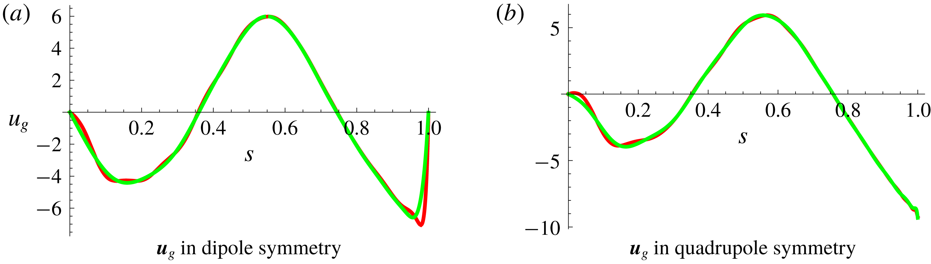
We note that Roberts & Wu (Reference Roberts and Wu2014) (their appendix B) proposed the presence of a singularity in
 $u_{g}$
at
 $s=1$
: for the dipole field,
 $B_{s}$
is always zero at
 $s=1$
due to symmetry, resulting in Taylor’s condition always being satisfied at the equator and therefore a nugatory role for the geostrophic flow at this point. In figure 11 (and also in the forthcoming figure 14), there is the suggestion of a boundary layer type structure in
 $u_{g}$
. In concert with Wu & Roberts (Reference Wu and Roberts2015) our solutions remain finite.
6.3 Force and energy balances in the
$\unicode[STIX]{x1D6FC}_{B}^{2}$
model

For the
 $\unicode[STIX]{x1D6FC}_{B}^{2}$
model we now examine the contribution of the different flow components in more detail. Following in the spirit of Taylor (Reference Taylor1963) temporarily, the time-differentiated Taylor integral
 $$\begin{eqnarray}\displaystyle \unicode[STIX]{x2202}_{t}{\mathcal{T}}=s\int _{C(s)}[\unicode[STIX]{x2202}_{t}\boldsymbol{J}\times \boldsymbol{B}+\boldsymbol{J}\times \unicode[STIX]{x2202}_{t}\boldsymbol{B}]\boldsymbol{\cdot }\hat{\unicode[STIX]{x1D753}}\,\text{d}z\,\text{d}\unicode[STIX]{x1D719}=0 & & \displaystyle\end{eqnarray}$$
can be split into several components as
 $$\begin{eqnarray}\displaystyle \unicode[STIX]{x0394}{\mathcal{T}}_{1} & = & \displaystyle s\int _{C(s)}[(\unicode[STIX]{x1D735}\times \unicode[STIX]{x0394}{\mathcal{I}}_{1})\times \boldsymbol{B}+(\unicode[STIX]{x1D735}\times \boldsymbol{B})\times \unicode[STIX]{x0394}{\mathcal{I}}_{1}]\boldsymbol{\cdot }\hat{\unicode[STIX]{x1D753}}\,\text{d}z\,\text{d}\unicode[STIX]{x1D719},\end{eqnarray}$$
 $$\begin{eqnarray}\displaystyle \unicode[STIX]{x0394}{\mathcal{T}}_{2} & = & \displaystyle s\int _{C(s)}[(\unicode[STIX]{x1D735}\times \unicode[STIX]{x0394}{\mathcal{I}}_{2})\times \boldsymbol{B}]\boldsymbol{\cdot }\hat{\unicode[STIX]{x1D753}}\,\text{d}z\,\text{d}\unicode[STIX]{x1D719},\end{eqnarray}$$
 $$\begin{eqnarray}\displaystyle \unicode[STIX]{x0394}{\mathcal{T}}_{3} & = & \displaystyle s\int _{C(s)}[(\!\unicode[STIX]{x1D735}\times \unicode[STIX]{x1D6FB}^{2}\boldsymbol{B}\times \boldsymbol{B}]\boldsymbol{\cdot }\hat{\unicode[STIX]{x1D753}}+[(\!\unicode[STIX]{x1D735}\times \boldsymbol{B}\times \unicode[STIX]{x1D6FB}^{2}\boldsymbol{B}]\boldsymbol{\cdot }\hat{\unicode[STIX]{x1D753}}\,\text{d}z\,\text{d}\unicode[STIX]{x1D719},\end{eqnarray}$$
which sum to zero at equilibrium, where the inductive secular variation contributions are
 $$\begin{eqnarray}\displaystyle \left.\begin{array}{@{}c@{}}\unicode[STIX]{x0394}{\mathcal{I}}_{1}=\unicode[STIX]{x1D735}\times [\boldsymbol{u}_{m}\times \boldsymbol{B}+{\mathcal{E}}],\\ \unicode[STIX]{x0394}{\mathcal{I}}_{2}=\unicode[STIX]{x1D735}\times [\boldsymbol{u}_{g}\times \boldsymbol{B}],\end{array}\right\} & & \displaystyle\end{eqnarray}$$
and we note that there is no second term in (6.4) arising for the geostrophic flow contribution by dint of the fact that it creates only azimuthal secular variation. We analyse these contributions in figure 12(a), which shows the leading-order Lorentz force balance in the
 $\hat{\unicode[STIX]{x1D753}}$
direction. There is a close balance between the
 $\boldsymbol{u}_{m}$
and
 $\boldsymbol{u}_{g}$
contributions, with the diffusion operating on a much longer time scale and contributing relatively little. Figure 12(b) illustrates the resulting Taylor integral of
 $\boldsymbol{B}$
versus the residue damping term,
 $\unicode[STIX]{x1D716}{\mathcal{L}}(\boldsymbol{u}_{g})=-\unicode[STIX]{x1D716}A(s)\boldsymbol{u}_{g}\boldsymbol{\cdot }\hat{\unicode[STIX]{x1D753}}$
. Here we see that the linear friction term is always small in comparison to the Taylor torque.
The contributions to the time-differentiated Taylor torque at
 $t=3$
in dipole symmetry for
 $\unicode[STIX]{x1D6FC}_{0}=18$
with
 $\unicode[STIX]{x1D712}_{T}^{2}=10^{-7}$
and
 $\unicode[STIX]{x1D716}=10^{-2}\sqrt{\unicode[STIX]{x1D712}_{T}^{2}}$
. (a) The leading-order balance in Taylor’s integral from the magnetic wind
 $\unicode[STIX]{x0394}{\mathcal{T}}_{1}$
(in red) and the geostrophic flow
 $\unicode[STIX]{x0394}{\mathcal{T}}_{2}$
(in green), with the diffusive term
 $\unicode[STIX]{x0394}{\mathcal{T}}_{3}$
(in black) making a minor contribution. (b) The normalized Taylor’s integral,
 ${\mathcal{T}}(s)/\langle \boldsymbol{B}^{2}\rangle$
, in blue alongside the damping term
 $\unicode[STIX]{x1D716}{\mathcal{L}}(\boldsymbol{u}_{g})$
in red.

Another useful diagnostic is the energy balance:
 $$\begin{eqnarray}\displaystyle \frac{\text{d}}{\text{d}t}\int _{V+\hat{V}}\frac{1}{2}\boldsymbol{B}^{2}\,\text{d}V=\int _{V+\hat{V}}\boldsymbol{B}\boldsymbol{\cdot }\frac{\unicode[STIX]{x2202}\boldsymbol{B}}{\unicode[STIX]{x2202}t}\,\text{d}V=\int _{V+\hat{V}}\boldsymbol{B}\boldsymbol{\cdot }[\unicode[STIX]{x1D735}\times (\boldsymbol{u}\times \boldsymbol{B}+{\mathcal{E}})-\unicode[STIX]{x1D702}^{\prime }\unicode[STIX]{x1D735}\times \unicode[STIX]{x1D735}\times \boldsymbol{B}]\,\text{d}V, & & \displaystyle \nonumber\\ \displaystyle & & \displaystyle\end{eqnarray}$$
and we define the following rate-of-work terms:
 $$\begin{eqnarray}\displaystyle W_{\unicode[STIX]{x1D6FC}_{B}} & = & \displaystyle \int _{V+\hat{V}}\boldsymbol{B}\boldsymbol{\cdot }\unicode[STIX]{x1D735}\times (\unicode[STIX]{x1D6FC}_{0}\unicode[STIX]{x1D6FC}_{B}\boldsymbol{B})\,\text{d}V,\end{eqnarray}$$
 $$\begin{eqnarray}\displaystyle W_{\unicode[STIX]{x1D6FB}^{2}\boldsymbol{B}} & = & \displaystyle \int _{V+\hat{V}}\boldsymbol{B}\boldsymbol{\cdot }\unicode[STIX]{x1D6FB}^{2}\boldsymbol{B}\,\text{d}V,\end{eqnarray}$$
 $$\begin{eqnarray}\displaystyle W_{\boldsymbol{u}_{m}} & = & \displaystyle \int _{V+\hat{V}}\boldsymbol{B}\boldsymbol{\cdot }\unicode[STIX]{x1D735}\times (\boldsymbol{u}_{m}\times \boldsymbol{B})\,\text{d}V,\end{eqnarray}$$
 $$\begin{eqnarray}\displaystyle W_{\boldsymbol{u}_{g}} & = & \displaystyle \int _{V+\hat{V}}\boldsymbol{B}\boldsymbol{\cdot }\unicode[STIX]{x1D735}\times (\boldsymbol{u}_{g}\times \boldsymbol{B})\,\text{d}V.\end{eqnarray}$$
An analysis of the equilibrium state for
 $\unicode[STIX]{x1D712}_{T}^{2}=10^{-7}$
,
 $\unicode[STIX]{x1D6FC}_{0}=18$
and
 $\unicode[STIX]{x1D716}=10^{-2}\sqrt{\unicode[STIX]{x1D712}_{T}^{2}}$
yields
 $W_{\unicode[STIX]{x1D6FC}_{B}}=-W_{\unicode[STIX]{x1D6FB}^{2}\boldsymbol{B}}\approx 80$
in dipole parity, whereas
 $W_{\unicode[STIX]{x1D6FC}_{B}}=-W_{\unicode[STIX]{x1D6FB}^{2}\boldsymbol{B}}\approx 90$
in quadrupole parity, while the contributions of
 $\boldsymbol{u}_{m}$
and
 $\boldsymbol{u}_{g}$
are expected to be zero and indeed are very small in the computation,
 $W_{\boldsymbol{u}_{m}}$
and
 $W_{\boldsymbol{u}_{g}}$
both being
 ${\sim}O(10^{-4}){-}O(10^{-5})$
.
6.4 Role of linear friction
In order to obtain a smooth and well-converged solution, a damping term has been applied in the computation. We compare the
 $\unicode[STIX]{x1D6FC}_{B}^{2}$
TS dynamo of
 $\unicode[STIX]{x1D6FC}_{0}=18$
with and without the damping term
 ${\mathcal{L}}(\boldsymbol{u}_{g})$
in a quadrupole symmetry class computation, where
 $\boldsymbol{u}_{g}$
is well defined everywhere. Both systems evolve with an identical energy trajectory and saturate at the same equilibrium state with the magnetic energy,
 $E=\langle \boldsymbol{B}^{2}\rangle /2=0.427$
(as in table 2); however there are differences in the solution of the geostrophic flow. Figure 13 illustrates the solution for
 $\boldsymbol{u}_{g}$
with (in red) and without (in green) the damping term,
 $\unicode[STIX]{x1D716}{\mathcal{L}}(\boldsymbol{u}_{g})=-\unicode[STIX]{x1D716}A(s)\boldsymbol{u}_{g}\boldsymbol{\cdot }\hat{\unicode[STIX]{x1D753}}$
. For the large-scale component of the geostrophic flow, the two solutions are in agreement; however, for the solution without the residue absorbing term, numerical error accumulates at the small scale and results an oscillatory solution. A very small residue damping term significantly improves the convergence and smoothness of the solution for the geostrophic flow.
The
 $\unicode[STIX]{x1D6FC}_{B}^{2}$
TS dynamo solutions of
 $\boldsymbol{u}_{g}$
as a function of
 $s$
for
 $\unicode[STIX]{x1D6FC}_{0}=18$
in Qp with (in red) and without (in green) the damping term
 $\unicode[STIX]{x1D716}{\mathcal{L}}(\boldsymbol{u}_{g})$
, where, for both solutions, the threshold value of the Taylor state is
 $\unicode[STIX]{x1D712}_{T}^{2}=10^{-7}$
and
 $\unicode[STIX]{x1D716}=10^{-2}\sqrt{\unicode[STIX]{x1D712}^{2}}$
.

The solution for
 $\boldsymbol{u}_{g}$
of the
 $\unicode[STIX]{x1D6FC}_{B}^{2}$
TS dynamo for different
 $\unicode[STIX]{x1D6FC}_{0}$
at equilibrium, where the black, red and green curves stand for the cases of
 $\unicode[STIX]{x1D6FC}_{0}=14.25$
, 16 and 18 in dipole symmetry (a) and for
 $\unicode[STIX]{x1D6FC}_{0}=14$
, 16 and 18 in quadrupole symmetry (b).

The total azimuthal flow for the
 $\unicode[STIX]{x1D6FC}_{B}^{2}$
TS dynamo at equilibrium for (a) dipole symmetry with
 $\unicode[STIX]{x1D6FC}_{0}=14.25$
, 16 and 18 and (b) for quadrupole symmetry with
 $\unicode[STIX]{x1D6FC}_{0}=14$
, 16 and 18.

6.5 Dominance of
$u_{g}$

We conclude this section by focusing on the azimuthal flow in the steady saturated solutions, noting that the geostrophic component is overwhelmingly dominant. We plot the solutions for
 $\boldsymbol{u}_{g}$
as a function of
 $\unicode[STIX]{x1D6FC}_{0}$
in figure 14 and the total azimuthal flow
 $u_{\unicode[STIX]{x1D719}}=[u_{m}]_{\unicode[STIX]{x1D719}}+u_{g}$
in figure 15 in the equilibrium states for the cases of
 $\unicode[STIX]{x1D6FC}_{0}=14.25,~16$
and 18 in the dipole symmetry and for
 $\unicode[STIX]{x1D6FC}_{0}=14,~16$
and 18 in the quadrupole symmetry. For all cases, we set
 $\unicode[STIX]{x1D712}_{T}^{2}=10^{-7}$
and
 $\unicode[STIX]{x1D716}=10^{-2}\sqrt{\unicode[STIX]{x1D712}_{T}^{2}}$
. For the
 $\unicode[STIX]{x1D6FC}_{B}^{2}$
dynamo, the flow is dominated by the geostrophic component. As we increase the driving force,
 $\unicode[STIX]{x1D6FC}_{0}$
, the intensity of the magnetostrophic and the geostrophic flow increases, although the flow pattern remains essentially the same. Table 3 records the root-mean-square values of the poloidal, toroidal and total flows. All solutions demonstrate spectral convergence, as shown in figure 16 for the energy spectra of
 $\boldsymbol{B}$
and
 $\boldsymbol{u}=\boldsymbol{u}_{m}+\boldsymbol{u}_{g}$
; more than eight decades of convergence in energy are found in the poloidal components, with slightly less in the toroidal components.
The poloidal and toroidal energy of
 $\boldsymbol{B}$
and
 $\boldsymbol{u}=\boldsymbol{u}_{m}+\boldsymbol{u}_{g}$
for the
 $\unicode[STIX]{x1D6FC}_{B}^{2}$
TS dynamo with
 $\unicode[STIX]{x1D6FC}_{0}=18$
in dipole (a–d) and quadrupole (e–h) symmetry classes. The triangles stand for the solution of
 $\unicode[STIX]{x1D712}_{T}^{2}=10^{-7}$
and
 $\unicode[STIX]{x1D716}=10^{-2}\sqrt{\unicode[STIX]{x1D712}_{T}^{2}}$
for both the Dp and Qp; and the diamonds are for
 $\unicode[STIX]{x1D712}_{T}^{2}=10^{-8}$
and
 $\unicode[STIX]{x1D716}=10^{-2}\sqrt{\unicode[STIX]{x1D712}_{T}^{2}}$
in dipole symmetry and for
 $\unicode[STIX]{x1D712}_{T}^{2}=10^{-9}$
and
 $\unicode[STIX]{x1D716}=10^{-2}\sqrt{\unicode[STIX]{x1D712}_{T}^{2}}$
in quadrupole symmetry.

The
 $L_{2}$
-norm of
 $\boldsymbol{u}_{m}$
of the poloidal and the toroidal components,
 $\sqrt{\int _{V}[\boldsymbol{u}_{m}]_{P}^{2}\,\text{d}V}$
and
 $\sqrt{\int _{V}[\boldsymbol{u}_{m}]_{T}^{2}\,\text{d}V}$
, and the norm of
 $\boldsymbol{u}_{g}$
,
 $\sqrt{\int _{V}\boldsymbol{ u}_{g}^{2}\,\text{d}V}$
, of the
 $\unicode[STIX]{x1D6FC}_{B}^{2}$
TS dynamo for different
 $\unicode[STIX]{x1D6FC}_{0}$
in dipole and quadrupole symmetries.

7 A Taylor state dynamo model driven by the
$\unicode[STIX]{x1D6FC}_{L}^{2}$
-effect

Most
 $\unicode[STIX]{x1D6FC}^{2}$
kinematic dynamos have real eigenvalues (monotonic growth), although their behaviour can change markedly when considering nonlinear equilibration within the Taylor regime (Hollerbach & Ierley Reference Hollerbach and Ierley1991). In the previous section, we showed that the Braginsky TS model saturates in a steady state, but here we describe a different TS
 $\unicode[STIX]{x1D6FC}^{2}$
dynamo, driven by the
 $\unicode[STIX]{x1D6FC}_{L}$
term of (5.3), whose nonlinear evolution is oscillatory in time. The kinematic behaviour of this dynamo was described in § 5 and consists of two pairs of active dynamo regions with opposite polarities, the dominant region being located at low latitude as seen in the kinematic eigenfunction of figure 6(b). However, when Taylor’s constraint is enforced, the structure changes considerably.
The energy evolution of the
 $\unicode[STIX]{x1D6FC}_{L}^{2}$
Taylor state dynamo for
 $\unicode[STIX]{x1D6FC}_{L}=13,~14$
and 15 in red, green and blue respectively.
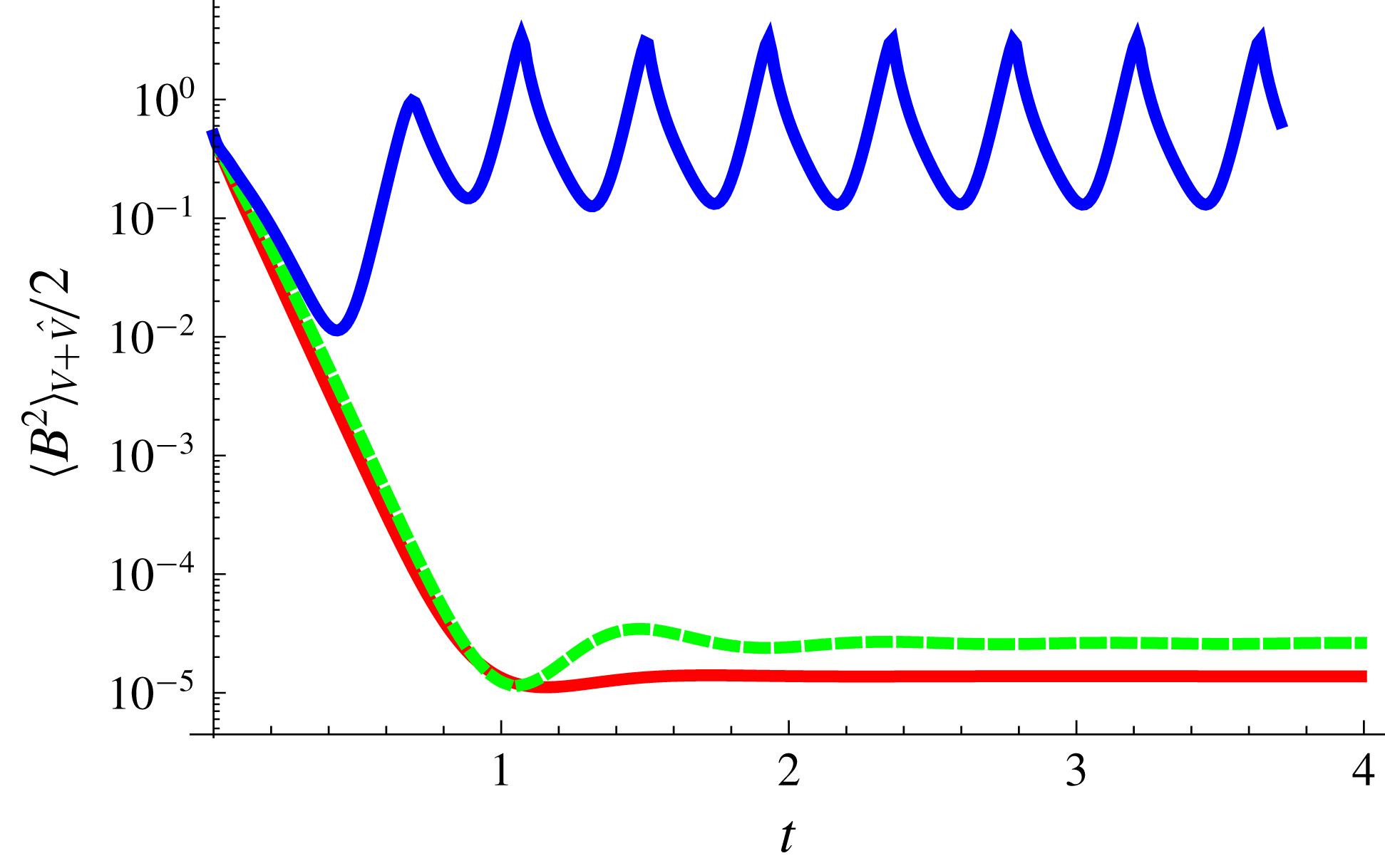
Figure 17 shows the energy evolution of the dynamo system for
 $\unicode[STIX]{x1D6FC}_{0}=13,~14$
and 15. At low driving,
 $\unicode[STIX]{x1D6FC}_{0}=13$
and 14, the dynamo system is stationary and dominated by the dynamo region at low latitudes, as shown in figure 18. For these values, the magnetic field distribution is similar to the kinematic case and the flow is dominated by the geostrophic component: compare figures 6(b) and 18. A bifurcation occurs in the range
 $14<\unicode[STIX]{x1D6FC}_{0}<15$
, such that the dynamo region at high latitudes becomes strong enough to interact with the dominant region at low latitudes. The TS dynamo now oscillates periodically with a period of approximately 40 % of the magnetic decay time. Figure 19 shows contours of
 $\boldsymbol{B}$
and
 $\boldsymbol{u}_{m}+\boldsymbol{u}_{g}$
in the maximum, middle and minimum energy states. In the maximum energy state (figure 19
a), the dynamo solution is similar to the solution of
 $\unicode[STIX]{x1D6FC}_{0}=14$
but with stronger intensity, while clearly showing that the dynamo is dominated by the dynamo region at low latitude. Simultaneously, the weak dynamo region grows and amplifies the magnetic field of the opposite polarity in the
 $B_{\unicode[STIX]{x1D719}}$
component (figure 19
b). When the energy reaches a minimum, the magnetic field
 $B_{\unicode[STIX]{x1D719}}$
polarity has reversed completely, while the poloidal field is dominated by an octupole rather than a dipole component (the dipole energy has dropped to approximately one-hundredth of its peak value). We still find that the flow is dominated by the geostrophic component and varies together with the magnetic field, although we note that the relative role of the geostrophic flow (compared with the ageostrophic flow) is time-dependent, for example, taking a more dominant role in the minimal energy state (see also Fearn & Rahman Reference Fearn and Rahman2004). The flow is enslaved to the magnetic field, where the energy of
 $\boldsymbol{u}_{m}$
and
 $\boldsymbol{u}_{g}$
and the energy of
 $\boldsymbol{B}$
reach maxima and minima simultaneously. Values of the magnetic energy in this
 $\unicode[STIX]{x1D6FC}_{0}=15$
oscillatory state are given in table 4.
The contours of
 $\boldsymbol{B}$
and
 $\boldsymbol{u}_{m}+\boldsymbol{u}_{g}$
of the
 $\unicode[STIX]{x1D6FC}_{L}^{2}$
TS dynamo for
 $\unicode[STIX]{x1D6FC}_{0}=14$
in dipole symmetry.

The contours of
 $\boldsymbol{B}$
and
 $\boldsymbol{u}_{m}+\boldsymbol{u}_{g}$
of the
 $\unicode[STIX]{x1D6FC}_{L}^{2}$
TS dynamo for
 $\unicode[STIX]{x1D6FC}_{0}=15$
in dipole symmetry in the maximal, middle and minimal energy states. (a) The maximal magnetic energy state at
 $t=1.07$
. (b) The middle magnetic energy state at
 $t=1.19$
. (c) The minimal magnetic energy state at
 $t=1.32$
.

The poloidal, toroidal and total energy of the
 $\unicode[STIX]{x1D6FC}_{L}^{2}$
Taylor state dynamo for different
 $\unicode[STIX]{x1D6FC}_{0}$
in dipole symmetry, where ‘min’ and ‘max’ indicate the dynamo state with minimal and maximal magnetic energy and ‘mid’ is the state at the time snapshot at the middle of the ‘min’ and ‘max’ states.

In quadrupole symmetry, the TS dynamo solution remains stationary up to
 $\unicode[STIX]{x1D6FC}_{0}=15$
but with energy
 $E_{P}=5.14$
,
 $E_{T}=2.1$
and
 $E=7.24$
for the poloidal, toroidal and total magnetic energy, approximately twice as large as the maximal energy state of the dipole case. We have not investigated higher values to see if there is also a transition to an oscillatory state.
We find it instructive to compute the same diagnostics as before in terms of force and energy balances. Figure 20(a) shows the leading-order net Lorentz force balance (see (6.3)–(6.5)) and figure 20(b) compares the Taylor torque to the damping term. In terms of the energy balance, figure 21 illustrates the rate of energy variation due to the
 $\unicode[STIX]{x1D6FC}_{L}$
-effect,
 $\unicode[STIX]{x1D6FB}^{2}B$
,
 $\boldsymbol{u}_{m}$
and
 $\boldsymbol{u}_{g}$
terms. The
 $\unicode[STIX]{x1D6FC}_{L}^{2}$
-effect is completely balanced by the magnetic diffusion process, while the energy contribution from the
 $\boldsymbol{u}_{m}$
and
 $\boldsymbol{u}_{g}$
terms are five to six orders of magnitude smaller than these leading terms. Note that, since the dynamo is not steady, we do not expect the exact cancellation that we previously saw in the
 $\unicode[STIX]{x1D6FC}_{B}^{2}$
dynamo energetics. We can again demonstrate the excellent spectral convergence our scheme is able to achieve; the energies as a function of spherical harmonic degree
 $l$
are shown in figure 22 for
 $\boldsymbol{B}$
and
 $\boldsymbol{u}=\boldsymbol{u}_{m}+\boldsymbol{u}_{g}$
when we set
 $\unicode[STIX]{x1D6FC}_{0}=15$
and observe the maximal energy state. We see 12 orders of magnitude of decrease in the energies. The calculations were performed with spatial and temporal resolutions set to be
 $L_{B}=50$
,
 $L_{u_{m}}=100$
,
 $N_{u_{g}}=50$
and
 $\unicode[STIX]{x0394}t=10^{-6}$
. The threshold value is
 $\unicode[STIX]{x1D712}_{T}^{2}=10^{-7}$
with the damping parameter
 $\unicode[STIX]{x1D716}=10^{-2}\sqrt{\unicode[STIX]{x1D712}_{T}^{2}}$
.
Plot of the Taylor torque at
 $t=1.07$
in the maximum magnetic energy state for
 $\unicode[STIX]{x1D6FC}_{0}=15$
with
 $\unicode[STIX]{x1D712}_{T}^{2}=10^{-7}$
and
 $\unicode[STIX]{x1D716}=10^{-2}\sqrt{\unicode[STIX]{x1D712}_{T}^{2}}$
. (a) The leading-order balance in the time derivative of the Taylor torque from the magnetic wind
 $\unicode[STIX]{x0394}{\mathcal{T}}_{1}$
(in red) and the geostrophic flow
 $\unicode[STIX]{x0394}{\mathcal{T}}_{2}$
(in green); the very small diffusive contribution
 $\unicode[STIX]{x0394}{\mathcal{T}}_{3}$
is omitted. (b) The normalized Taylor’s integral,
 ${\mathcal{T}}(s)/\langle \boldsymbol{B}^{2}\rangle$
, in blue, alongside the damping term
 $\unicode[STIX]{x1D716}{\mathcal{L}}(\boldsymbol{u}_{g})$
, in red.

Plot of
 $\text{d}E/\text{d}t$
of the
 $\unicode[STIX]{x1D6FC}_{L}^{2}$
TS dynamo in dipole symmetry, where the black, purple, green and red curves correspond to the
 $\unicode[STIX]{x1D6FC}$
-effect, magnetic diffusion,
 $\boldsymbol{u}_{m}$
and
 $\boldsymbol{u}_{g}$
field.

The poloidal (red triangles) and toroidal (green diamonds) energy spectra of the magnetic field and total velocity field,
 $\boldsymbol{u}=\boldsymbol{u}_{m}+\boldsymbol{u}_{g}$
, for the
 $\unicode[STIX]{x1D6FC}_{L}^{2}$
TS dynamo in dipole symmetry as a function of the spherical harmonic degree,
 $l$
, at the maximal magnetic energy state.

8 A Taylor state dynamo model driven by the
$\unicode[STIX]{x1D6FC}_{B}\unicode[STIX]{x1D714}_{B}$
-effect

As a last example, we study the axisymmetric Taylor state model driven by an
 $\unicode[STIX]{x1D6FC}_{B}\unicode[STIX]{x1D714}_{B}$
-effect, where the system is governed by (5.9) and the
 $\unicode[STIX]{x1D6FC}$
- and
 $\unicode[STIX]{x1D714}$
-effects are defined in (5.2) and (5.4). Roberts (Reference Roberts1972) previously discovered the onset of dynamo action for this system at
 $\unicode[STIX]{x1D6FC}_{c}=-\unicode[STIX]{x1D714}_{T}=206$
; Wu & Roberts (Reference Wu and Roberts2015) also found Taylor states above
 $\unicode[STIX]{x1D6FC}_{T}=-\unicode[STIX]{x1D714}_{T}=420$
.
We choose
 $\hat{\boldsymbol{S}}_{(1,1,0)}$
and
 $\hat{\boldsymbol{S}}_{(1,2,0)}$
as the initial conditions for the
 $\unicode[STIX]{x1D6FC}_{B}\unicode[STIX]{x1D714}_{B}$
TS dynamo in dipole and quadrupole symmetry classes, respectively, and forward integrate dynamos in time for the system with
 $\unicode[STIX]{x1D6FC}_{0}=-\unicode[STIX]{x1D714}_{0}=425$
, a value slightly above the known onset value. We use the solution at
 $t=5$
(decay times) as the initial condition for larger driving force models,
 $\unicode[STIX]{x1D6FC}_{0}=-\unicode[STIX]{x1D714}_{0}=450$
and 500. Figure 23 illustrates the evolution of the magnetic energy of the dynamo systems as a function of time for
 $\unicode[STIX]{x1D6FC}_{0}=-\unicode[STIX]{x1D714}_{0}=425,~450$
and 500 for both symmetry classes. The saturated energy increases as we increase the driving, while the intensity of the flow,
 $\boldsymbol{u}_{m}$
and
 $\boldsymbol{u}_{g}$
varies in phase with the variation of the magnetic field. We find that the oscillation frequency of this system increases as the driving force is increased. None of the dynamos are exactly sinusoidal in figure 23(a), but the two cases of weakest driving are periodic. The behaviour for the strongest driving appears to be entirely consistent with the results of Wu & Roberts (Reference Wu and Roberts2015). The quadrupolar symmetry case is not reported by Wu & Roberts (Reference Wu and Roberts2015) but in our calculations shows a marked periodic behaviour for the two lowest
 $\unicode[STIX]{x1D6FC}_{0}$
cases, in contrast to the much more chaotic behaviour at
 $\unicode[STIX]{x1D6FC}_{0}=500$
.
The energy evolution of the
 $\unicode[STIX]{x1D6FC}_{B}\unicode[STIX]{x1D714}_{B}$
Taylor state dynamo with
 $\unicode[STIX]{x1D6FC}_{0}=-\unicode[STIX]{x1D714}_{0}=425,~450$
and 500, respectively, in blue, green and dashed red in Dp (a) and Qp (b).

In terms of inductive effects, the
 $\unicode[STIX]{x1D6FC}_{B}\unicode[STIX]{x1D714}_{B}$
dynamo oscillates as a result of the competition between the
 $\unicode[STIX]{x1D6FC}_{B}$
- and
 $\unicode[STIX]{x1D714}_{B}$
-effects. Strong magnetic fields are generated within the regions to which the
 $\unicode[STIX]{x1D6FC}_{B}$
-effect and
 $\unicode[STIX]{x1D714}_{B}$
-effects are localized with different polarities and drift outwards. At the intersections between two strong field patches, the flow has the largest magnitude and shear. In the dipole symmetry, we plot contours of the magnetic field and the magnetostrophic flow,
 $\boldsymbol{u}_{m}$
for
 $\unicode[STIX]{x1D6FC}_{0}=-\unicode[STIX]{x1D714}_{0}=500$
in figure 24 and
 $\unicode[STIX]{x1D6FC}_{0}=-\unicode[STIX]{x1D714}_{0}=450$
for the quadrupole field in figure 25. The solutions for the geostrophic flow (figure 26) and the zonal flow
 $[u_{m}]_{\unicode[STIX]{x1D719}}+u_{g}$
(figure 27) both show minor changes to the flow structure between times of magnetic energy maxima and minima.
Contours of
 $\boldsymbol{B}$
and
 $\boldsymbol{u}_{m}$
of the
 $\unicode[STIX]{x1D6FC}_{B}\unicode[STIX]{x1D714}_{B}$
Taylor state dynamo with
 $\unicode[STIX]{x1D6FC}_{0}=-\unicode[STIX]{x1D714}_{0}=500$
in minimum and maximum energy states in dipole symmetry: (a) at the minimum energy state at
 $t=1.56$
; (b) at the maximum energy state at
 $t=1.51$
.

Contours of
 $\boldsymbol{B}$
and
 $\boldsymbol{u}_{m}$
of the
 $\unicode[STIX]{x1D6FC}_{B}\unicode[STIX]{x1D714}_{B}$
Taylor state dynamo with
 $\unicode[STIX]{x1D6FC}_{0}=-\unicode[STIX]{x1D714}_{0}=450$
in minimum and maximum energy states in quadrupole symmetry: (a) at the minimum energy state at
 $t=1.67$
; (b) at the maximum energy state at
 $t=1.73$
.

The solution for
 $\boldsymbol{u}_{g}$
in the minimum (red) and the maximum (green) magnetic energy states as a function of
 $s$
for (a)
 $\unicode[STIX]{x1D6FC}_{0}=-\unicode[STIX]{x1D714}_{0}=500$
in dipole symmetry and (b)
 $\unicode[STIX]{x1D6FC}_{0}=-\unicode[STIX]{x1D714}_{0}=450$
in quadrupole symmetry.

Contours of the zonal flow,
 $[u_{m}]_{\unicode[STIX]{x1D719}}+u_{g}$
, for
 $\unicode[STIX]{x1D6FC}_{0}=-\unicode[STIX]{x1D714}_{0}=500$
in dipole symmetry and
 $\unicode[STIX]{x1D6FC}_{0}=-\unicode[STIX]{x1D714}_{0}=450$
in quadrupole symmetry at the minimal (a,c) and maximal (b,d) magnetic energy state.

We again dissect the forces in a similar way to previously in figure 28(a). We need to slightly redefine the quantity
 $\unicode[STIX]{x0394}{\mathcal{I}}_{1}$
for this new system, but it remains analogous to the previous definition; in this case
 $$\begin{eqnarray}\displaystyle {\mathcal{I}}_{1}=\unicode[STIX]{x1D735}\times [\boldsymbol{u}_{m}\times \boldsymbol{B}+\unicode[STIX]{x1D6FC}_{0}\unicode[STIX]{x1D6FC}_{B}\hat{\boldsymbol{T}}+\unicode[STIX]{x1D714}_{0}(r\sin \unicode[STIX]{x1D703}\,\unicode[STIX]{x1D714}_{B})\hat{\unicode[STIX]{x1D753}}\times \hat{\boldsymbol{S}}], & & \displaystyle\end{eqnarray}$$
but the definitions
 $\unicode[STIX]{x0394}{\mathcal{T}}_{i}$
of (6.3)–(6.5) remain. The behaviour of the
 $\unicode[STIX]{x0394}{\mathcal{T}}_{i}$
in figure 28(a) follows the familiar pattern of cancellation seen before, and again, the damping effect in figure 28(b) remains negligible.
Plot of the Taylor torque in the
 $\unicode[STIX]{x1D6FC}_{B}\unicode[STIX]{x1D714}_{B}$
TS dynamo for the dipole symmetry at the maximal magnetic energy state when
 $\unicode[STIX]{x1D6FC}_{0}=-\unicode[STIX]{x1D714}_{0}=500$
with
 $\unicode[STIX]{x1D712}_{T}^{2}=10^{-7}$
and
 $\unicode[STIX]{x1D716}=10^{-2}\sqrt{\unicode[STIX]{x1D712}_{T}^{2}}$
. (a) The leading-order balance in the time derivative of Taylor integral from the magnetic wind
 $\unicode[STIX]{x0394}{\mathcal{T}}_{1}$
(in red) and the geostrophic flow
 $\unicode[STIX]{x0394}{\mathcal{T}}_{2}$
(in green); the very small diffusive contribution
 $\unicode[STIX]{x0394}{\mathcal{T}}_{3}$
is omitted. (b) The normalized Taylor’s integral,
 ${\mathcal{T}}/\langle \boldsymbol{B}^{2}\rangle$
, in blue, alongside the damping term
 $\unicode[STIX]{x1D716}{\mathcal{L}}(\boldsymbol{u}_{g})$
, in red.

We again analyse the energy balance as before. Figure 29 illustrates the changes in the magnetic energy due to the
 $\unicode[STIX]{x1D6FC}_{B}$
,
 $\unicode[STIX]{x1D714}_{B}$
,
 $\unicode[STIX]{x1D6FB}^{2}B$
,
 $\boldsymbol{u}_{m}$
and
 $\boldsymbol{u}_{g}$
terms. The
 $\unicode[STIX]{x1D6FC}_{B}$
-effect and the magnetic diffusion process are the leading-order terms and balance each other. The energy contributions from
 $\boldsymbol{u}_{m}$
and
 $\boldsymbol{u}_{g}$
are six or seven orders of magnitude smaller than the leading terms.
Plots of
 $\text{d}E/\text{d}t$
of the
 $\unicode[STIX]{x1D6FC}_{B}\unicode[STIX]{x1D714}_{B}$
TS dynamo for both dipole and quadrupole symmetries, where the black, purple, green, red and blue curves correspond to the
 $\unicode[STIX]{x1D6FC}$
-effect, magnetic diffusion,
 $\boldsymbol{u}_{m}$
,
 $\boldsymbol{u}_{g}$
and
 $\unicode[STIX]{x1D714}$
-effect field.

We end this section with the usual demonstration of spectral convergence in figure 30. The
 $\unicode[STIX]{x1D6FC}_{B}\unicode[STIX]{x1D714}_{B}$
model considered here was computed with
 $L_{B}=40$
,
 $L_{u_{m}}=80$
,
 $N_{u_{g}}=40$
and
 $\unicode[STIX]{x0394}t=10^{-6}$
.
The poloidal (red triangles) and toroidal (green diamonds) energy of
 $\boldsymbol{B}$
and
 $\boldsymbol{u}=\boldsymbol{u}_{m}+\boldsymbol{u}_{g}$
for the
 $\unicode[STIX]{x1D6FC}_{B}\unicode[STIX]{x1D714}_{B}$
TS dynamo in the maximum magnetic energy state at
 $t=1.51$
with
 $\unicode[STIX]{x1D6FC}_{0}=-\unicode[STIX]{x1D714}_{0}=500$
,
 $\unicode[STIX]{x1D712}_{T}^{2}=10^{-7}$
and
 $\unicode[STIX]{x1D716}=10^{-2}\sqrt{\unicode[STIX]{x1D712}_{T}^{2}}$
, as a function of spherical harmonic degree,
 $l$
, in dipole symmetry.

9 Discussion and conclusions
We have developed a comprehensive methodology for evolving the Taylor state dynamo system based on the paradigm of optimal control, and demonstrated its effectiveness through examples of axisymmetric Taylor state dynamos driven by mean-field effects. The solutions we obtain are smooth, accurate and well converged. It is our view that obtaining solutions to the inviscid problem, in which the Ekman number
 $E=0$
, is a worthy step towards understanding real planetary cores (described by
 $E=O(10^{-15})$
), and certainly the inviscid problem can be seen as an extreme point that complements the set of conventional viscous dynamos, currently reaching no lower than
 $E=O(10^{-7})$
. True planetary behaviour necessarily lives between these two dynamical regimes. Together with the seminal work of Wu & Roberts (Reference Wu and Roberts2015), we have successfully enlarged the domain of planetary behaviours that can be addressed by numerical calculation. In all our models, the geostrophic flow dominates the ageostrophic flow, in agreement with some theories (Braginsky Reference Braginsky1964), but in contrast to the current state of the art of conventional weakly viscous dynamos (Christensen & Wicht Reference Christensen and Wicht2015).
As we have stressed throughout this paper, the algorithm developed is inherently 3D. However, we have applied it only to axisymmetric examples in order to compare against other published work: in particular, we find in general close agreement with the results of Wu & Roberts (Reference Wu and Roberts2015). It is worth noting, however, that the algorithm of Wu & Roberts (Reference Wu and Roberts2015) cannot be extended to three dimensions because it is dependent on the form of the Taylor integral specialized to axisymmetry. Thus, what we present here is a promising new, entirely general, method for computing 3D Taylor state dynamos. Our framework can further be extended to include viscous effects within the thin Ekman boundary layers, while neglecting viscosity within the bulk of the domain (Braginsky Reference Braginsky1964).
In a magnetostrophic balance, the Taylor integral is necessarily exactly zero. However, in numerical computations, this condition is difficult to achieve, a phenomenon already observed by Wu & Roberts (Reference Wu and Roberts2015). Therefore, we introduce a threshold,
 $\unicode[STIX]{x1D712}_{T}^{2}$
, as an acceptance criterion. When the Taylicity (recall this is the normalized misfit,
 $\mathbb{T}$
) is smaller than this value, we accept that the solution is in a Taylor state. In this study, we tested several cases for
 $\unicode[STIX]{x1D712}_{T}^{2}=10^{-6}{-}10^{-8}$
and found that the saturated states agree with one another, suggesting that our models were independent of
 $\unicode[STIX]{x1D712}_{T}^{2}$
and therefore also describe the Taylor state end-member for which
 $\unicode[STIX]{x1D712}_{T}^{2}=0$
. However, whether a 3D convection-driven dynamo remains similarly insensitive to the value of
 $\unicode[STIX]{x1D712}_{T}^{2}$
(for
 $\unicode[STIX]{x1D712}_{T}^{2}\ll 1$
) remains a topic for future investigation.
We found that stably evolving a dynamo system close to the Taylor manifold to be a delicate task. In our numerical experiments, when
 $\unicode[STIX]{x0394}t$
is set too large and
 $\unicode[STIX]{x1D712}_{T}^{2}$
is too small, the computation becomes very expensive, as reflected in the number of iterations within the optimization loop increasing dramatically from 0–3 to
 $O(100)$
at each time step. Our numerical work further revealed that it was necessary to introduce a linear damping term in our computations, as, without it, the solution for the geostrophic flow
 $\boldsymbol{u}_{g}$
became noisy. However, in our experiments, we ensured that the numerical damping term, in the optimized state, was very small compared to the Taylor integral, and thus acted only as a numerical tool for approaching the inviscid state, without affecting the structure of the solution. The questions of how to choose the threshold
 $\unicode[STIX]{x1D712}_{T}^{2}$
with respect to
 $\unicode[STIX]{x0394}t$
, and how to objectively control the optimal damping mechanism, remain open.
The optimal solution for
 $\boldsymbol{u}_{g}$
is computed via a gradient-based optimization method, the limited-memory BFGS algorithm (Nocedal & Wright Reference Nocedal and Wright2006). The gradient,
 $\unicode[STIX]{x1D735}_{\boldsymbol{u}_{g}}\unicode[STIX]{x1D712}^{2}$
, is computed via an adjoint method, which is efficient and accurate up to machine procession, and the second-derivative Hessian matrix is estimated and updated at each iteration by the BFGS routine, based on previous search directions. Therefore, our method is a first-order method. In the future we may make use of methods that can compute the Hessian term from first principles for a particular time-stepping scheme. For example, for the 2D cases considered here and the AB2 time-stepping scheme,
 $\boldsymbol{B}$
and
 $\unicode[STIX]{x1D735}\times \boldsymbol{B}$
can always be written as
 $$\begin{eqnarray}\displaystyle \boldsymbol{B}_{t+\unicode[STIX]{x0394}t} & = & \displaystyle \boldsymbol{C}+\frac{3\unicode[STIX]{x0394}t}{2}L_{1}(\boldsymbol{u}_{g})\end{eqnarray}$$
and
 $$\begin{eqnarray}\displaystyle \unicode[STIX]{x1D735}\times \boldsymbol{B}_{t+\unicode[STIX]{x0394}t}=\unicode[STIX]{x1D735}\times \boldsymbol{C}+\frac{3\unicode[STIX]{x0394}t}{2}L_{2}(\boldsymbol{u}_{g}), & & \displaystyle\end{eqnarray}$$
where
 $\boldsymbol{C}$
is a known function of
 $\boldsymbol{B}_{t}$
and
 $\boldsymbol{u}_{m}$
, and
 $L_{1}(\boldsymbol{u}_{g})=\unicode[STIX]{x1D735}\times (\boldsymbol{u}_{g}\times \boldsymbol{B}_{t})$
and
 $L_{2}(\boldsymbol{u}_{g})=\unicode[STIX]{x1D735}\times \unicode[STIX]{x1D735}\times (\boldsymbol{u}_{g}\times \boldsymbol{B}_{t})$
. Each entry of the Hessian matrix,
 ${\mathcal{H}}_{i,j}$
, can be written as
 $$\begin{eqnarray}\displaystyle {\mathcal{H}}_{i,j}=\frac{9\unicode[STIX]{x0394}t^{2}}{4}\int _{V}L_{1}(\unicode[STIX]{x1D6EC}_{i})L_{2}(\unicode[STIX]{x1D6EC}_{j})\,\text{d}V & & \displaystyle\end{eqnarray}$$
and
 $\boldsymbol{u}_{g}=\boldsymbol{u}_{g}^{est}-{\mathcal{H}}^{-1}\unicode[STIX]{x1D735}_{\boldsymbol{u}_{g}}\unicode[STIX]{x1D712}^{2}$
, where
 $\boldsymbol{u}_{g}^{est}$
is the previous estimate.
Much remains to be done, not least the adaptation of the present ideas to the problem of thermal convection in a 3D setting. The only remaining small parameter in this problem is the Roberts number
 $q$
, which has values of
 $O(10^{-5})$
in the Earth. Present-day models face the same challenge of handling small amounts of thermal diffusion, and as a result computations tend to favour
 $q\sim O(10^{-1})$
or larger. Oceanographic dynamics face analogous problems, and developments from this field (e.g. Arakawa & Lamb Reference Arakawa and Lamb1981) may prove to be transferable. Nevertheless, even at
 $q\sim O(1)$
it is expected that results and dynamics may differ substantially from the currently computed dynamos.
Acknowledgements
This work was supported by SNF grants 200020_143596 and 200021_163163, by ERC grant 247303 (MFECE) and by NERC grant NE/G014043/1. A.J. is grateful to Dr C. Pringle for a helpful discussion that provided clarity at a critical time in the project. J. Luo is thanked for his careful reading of the manuscript. Part of this work was performed when A.J. was a visitor at the Bullard Laboratories, University of Cambridge. He thanks the Drum building members, and particularly Professor N. J. White, for the hospitality shown. We thank Professor G. Ierley for numerous discussions and encouragement, and for providing the proof of appendix F. The manuscript benefited from the reviews of Professor P. H. Roberts and two anonymous reviewers.
Appendix A. Symmetry classes of the Taylor state system
The vector (
 $\boldsymbol{u}_{m}$
,
 $\boldsymbol{u}_{g}$
and
 $\boldsymbol{B}$
) can be categorized in equatorially symmetric and antisymmetric classes, also known as the quadrupole and dipole symmetries. Let us denote by
 $E^{S}$
and
 $E^{A}$
two sets of scalar functions and by
 $\boldsymbol{E}^{S}$
and
 $\boldsymbol{E}^{A}$
two sets of vector functions of the symmetric and antisymmetric classes labelled by the superscripts
 $S$
and
 $A$
. In spherical coordinates,
 $E^{S}$
and
 $E^{A}$
, respectively, satisfy (Gubbins & Zhang Reference Gubbins and Zhang1993)
(i)
$E^{S}(r,\unicode[STIX]{x1D703},\unicode[STIX]{x1D719})=E^{S}(r,\unicode[STIX]{x03C0}-\unicode[STIX]{x1D703},\unicode[STIX]{x1D719})$
,(ii)
$E^{A}(r,\unicode[STIX]{x1D703},\unicode[STIX]{x1D719})=-E^{A}(r,\unicode[STIX]{x03C0}-\unicode[STIX]{x1D703},\unicode[STIX]{x1D719})$
,


and
 $\boldsymbol{E}^{S}$
and
 $\boldsymbol{E}^{A}$
, respectively, satisfy
(i)
$[E_{r}^{S},E_{\unicode[STIX]{x1D703}}^{S},E_{\unicode[STIX]{x1D719}}^{S}](r,\unicode[STIX]{x1D703},\unicode[STIX]{x1D719})=[E_{r}^{S},-E_{\unicode[STIX]{x1D703}}^{S},E_{\unicode[STIX]{x1D719}}^{S}](r,\unicode[STIX]{x03C0}-\unicode[STIX]{x1D703},\unicode[STIX]{x1D719})$
,(ii)
$[E_{r}^{A},E_{\unicode[STIX]{x1D703}}^{A},E_{\unicode[STIX]{x1D719}}^{A}](r,\unicode[STIX]{x1D703},\unicode[STIX]{x1D719})=[-E_{r}^{A},E_{\unicode[STIX]{x1D703}}^{A},-E_{\unicode[STIX]{x1D719}}^{A}](r,\unicode[STIX]{x03C0}-\unicode[STIX]{x1D703},\unicode[STIX]{x1D719})$
.


The interactions of these functions follow a general rule; see table 5. Substituting the rules of table 5 into the governing equations (2.1) and (2.2), one has:
(i) if
$\boldsymbol{B}$
is
$\boldsymbol{E}^{S}/\boldsymbol{E}^{A}$
, the resulting Lorentz force is always
$\boldsymbol{E}^{S}$
, the magnetostrophic flow created by the Lorentz force is always
$\boldsymbol{E}^{S}$
and the induced magnetic field is
$\boldsymbol{E}^{S}/\boldsymbol{E}^{A}$
;(ii) if
$\boldsymbol{B}$
is mixed with both symmetry classes, all of Lorentz force, magnetostrophic flow and the induced magnetic fields are a mixture of two classes.


General rules of the interaction of different symmetry classes, where the symbol
 $\rightarrow$
stands for ‘result as’.

Appendix B. Functional differentiation and derivatives
We use the misfit,
 $\unicode[STIX]{x1D712}^{2}(\boldsymbol{u}_{g})$
, defined in (1.2) as a pertinent example of functional differentiation, where by definition the Gateaux differential of
 $\unicode[STIX]{x1D712}^{2}$
at
 $\boldsymbol{u}_{g}$
in the direction
 $\tilde{\boldsymbol{u}}_{g}$
reads
 $$\begin{eqnarray}\displaystyle D\unicode[STIX]{x1D712}^{2}(\boldsymbol{u}_{g})=\lim _{\unicode[STIX]{x1D70F}\rightarrow 0}\frac{\unicode[STIX]{x1D712}^{2}(\boldsymbol{u}_{g}+\unicode[STIX]{x1D70F}\tilde{\boldsymbol{u}}_{g})-\unicode[STIX]{x1D712}^{2}(\boldsymbol{u}_{g})}{\unicode[STIX]{x1D70F}}. & & \displaystyle\end{eqnarray}$$
In a Hilbert space, the differentiation in (B 1) can be written as the inner product,
 $$\begin{eqnarray}\displaystyle D\unicode[STIX]{x1D712}^{2}(\boldsymbol{u}_{g})=\int _{V}\unicode[STIX]{x1D735}_{\boldsymbol{u}_{g}}\unicode[STIX]{x1D712}^{2}\boldsymbol{\cdot }D\boldsymbol{u}_{g}\,\text{d}V, & & \displaystyle\end{eqnarray}$$
where
 $\int _{V}(\cdot )\,\text{d}V$
is the inner product and
 $\unicode[STIX]{x1D735}_{\boldsymbol{u}_{g}}\unicode[STIX]{x1D712}^{2}$
is the derivative of
 $\unicode[STIX]{x1D712}^{2}$
with respect to
 $\boldsymbol{u}_{g}$
. The differentiation of a function is a special case of the Gateaux differentiation, equation (B 2). For a function
 $F(\boldsymbol{r})$
defined in Euclidean space
 $(x,y,z)$
, its Gateaux derivative is equivalent to
 $\text{d}F(\boldsymbol{r})=\unicode[STIX]{x1D735}F(x,y,z)\cdot \text{d}\boldsymbol{r}$
.
Appendix C. Adjoint of the magnetic induction equation
In this section, we derive a general adjoint system of the electric and magnetic field; see also Namikawa & Matsushita (Reference Namikawa and Matsushita1970) for the less-general steady case. A derivation from a ‘primitive variables’ viewpoint is given in Chen et al. (Reference Chen, Herreman, Li, Livermore, Luo and Jackson2018). Working in dimensional quantities, the physical system is set up as follows. We consider diffusivities
 $\unicode[STIX]{x1D702}$
and
 $\hat{\unicode[STIX]{x1D702}}$
in
 $V$
and
 $\hat{V}$
, with the intention that we will let
 $\hat{\unicode[STIX]{x1D702}}\rightarrow \infty$
in order to achieve an insulating exterior. The boundary conditions that apply on
 $\unicode[STIX]{x2202}V$
, the boundary between
 $V$
and
 $\hat{V}$
, are
 $\boldsymbol{B}_{r=1_{-}}=\boldsymbol{B}_{r=1_{+}}$
while the tangential component of the electric field
 $\boldsymbol{E}_{\Vert }$
is continuous,
 $\hat{\boldsymbol{r}}\times \boldsymbol{E}_{r=1_{-}}=\hat{\boldsymbol{r}}\times \boldsymbol{E}_{r=1_{+}}$
; also
 $\boldsymbol{B}$
vanishes on the sphere
 $R_{\infty }$
at infinity,
 $\boldsymbol{B}\rightarrow 0|_{r\rightarrow \infty }$
.
We consider the adjoint of the induction equation subject to the divergenceless condition on
 $\boldsymbol{B}$
. Recall that throughout our treatment the inner product is based on integration over all space. We treat the contributions from
 $V$
and
 $\hat{V}$
separately, using the notation
 $\hat{\boldsymbol{B}}$
,
 $\hat{\boldsymbol{B}}^{\dagger }$
,
 $\hat{\boldsymbol{E}}$
and
 $\hat{\boldsymbol{E}}^{\dagger }$
for the magnetic and electric field and their adjoints in
 $\hat{V}$
.
The induction operator in
 $V$
is
 $$\begin{eqnarray}\displaystyle {\mathcal{I}}\boldsymbol{B}=\unicode[STIX]{x2202}_{t}\boldsymbol{B}-\unicode[STIX]{x1D735}\times (\boldsymbol{u}\times \boldsymbol{B}+\unicode[STIX]{x1D6FC}\boldsymbol{B})+\unicode[STIX]{x1D702}\unicode[STIX]{x1D735}\times \unicode[STIX]{x1D735}\times \boldsymbol{B}. & & \displaystyle\end{eqnarray}$$
We consider the integral over
 $V$
and over the time window
 $t\in [0,\unicode[STIX]{x0394}t]$
subject to the divergenceless condition imposed using Lagrange multiplier
 $p^{\dagger }$
:
 $$\begin{eqnarray}\displaystyle Q_{V}=\int _{0}^{\unicode[STIX]{x0394}t}\!\int _{V}\boldsymbol{B}^{\dagger }\boldsymbol{\cdot }{\mathcal{I}}\boldsymbol{B}\,\text{d}V+\int _{0}^{\unicode[STIX]{x0394}t}\!\int _{V}p^{\dagger }\unicode[STIX]{x1D735}\boldsymbol{\cdot }\boldsymbol{B}\,\text{d}V\,\text{d}t. & & \displaystyle\end{eqnarray}$$
Various manipulations lead to (Li et al. Reference Li, Jackson and Livermore2011)
 $$\begin{eqnarray}\displaystyle Q_{V} & = & \displaystyle \int _{0}^{\unicode[STIX]{x0394}t}\!\int _{V}\boldsymbol{B}\boldsymbol{\cdot }\left\{-\frac{\unicode[STIX]{x2202}\boldsymbol{B}^{\dagger }}{\unicode[STIX]{x2202}t}-\unicode[STIX]{x1D735}\times \boldsymbol{B}^{\dagger }\times \boldsymbol{u}-\unicode[STIX]{x1D6FC}(\boldsymbol{r})\unicode[STIX]{x1D735}\times \boldsymbol{B}^{\dagger }\right.\nonumber\\ \displaystyle & & \displaystyle -\left.\unicode[STIX]{x1D702}\unicode[STIX]{x1D6FB}^{2}\boldsymbol{B}^{\dagger }+[\unicode[STIX]{x1D6FF}(t-\unicode[STIX]{x0394}t)-\unicode[STIX]{x1D6FF}(t)]\boldsymbol{B}^{\dagger }-\unicode[STIX]{x1D735}p^{\dagger }\right\}\,\text{d}V\,\text{d}t+S,\end{eqnarray}$$
where
 $$\begin{eqnarray}\displaystyle S=\int _{0}^{\unicode[STIX]{x0394}t}\!\int _{\unicode[STIX]{x2202}V}[\boldsymbol{B}^{\dagger }\times (\boldsymbol{u}\times \boldsymbol{B})+\unicode[STIX]{x1D6FC}(\boldsymbol{B}^{\dagger }\times \boldsymbol{B})+\unicode[STIX]{x1D702}\boldsymbol{B}\times \unicode[STIX]{x1D735}\times \boldsymbol{B}^{\dagger }-\unicode[STIX]{x1D702}\boldsymbol{B}^{\dagger }\times \unicode[STIX]{x1D735}\times \boldsymbol{B}+p^{\dagger }\boldsymbol{B}]\boldsymbol{\cdot }\hat{\boldsymbol{r}}\,\text{d}S\,\text{d}t. & & \displaystyle \nonumber\\ \displaystyle & & \displaystyle\end{eqnarray}$$
The electric field in
 $V$
is
 $$\begin{eqnarray}\displaystyle \boldsymbol{E}=\unicode[STIX]{x1D702}\unicode[STIX]{x1D735}\times \boldsymbol{B}-\boldsymbol{u}\times \boldsymbol{B}-\unicode[STIX]{x1D6FC}\boldsymbol{B}, & & \displaystyle\end{eqnarray}$$
which we identify with the terms in (C 4), so that
 $$\begin{eqnarray}\displaystyle S=\int _{0}^{\unicode[STIX]{x0394}t}\!\int _{\unicode[STIX]{x2202}V}[-\boldsymbol{B}^{\dagger }\times \boldsymbol{E}+\unicode[STIX]{x1D702}\boldsymbol{B}\times \unicode[STIX]{x1D735}\times \boldsymbol{B}^{\dagger }+p^{\dagger }\boldsymbol{B}]\boldsymbol{\cdot }\hat{\boldsymbol{r}}\,\text{d}S\,\text{d}t. & & \displaystyle\end{eqnarray}$$
Note that only the horizontal electric field enters this surface integral since
 $\hat{\boldsymbol{r}}\boldsymbol{\cdot }\boldsymbol{B}^{\dagger }\times \boldsymbol{E}=\boldsymbol{E}_{\Vert }\boldsymbol{\cdot }\hat{\boldsymbol{r}}\times \boldsymbol{B}^{\dagger }$
, so that
 $S$
becomes
 $$\begin{eqnarray}\displaystyle S=\int _{0}^{\unicode[STIX]{x0394}t}\!\int _{\unicode[STIX]{x2202}V}[-\boldsymbol{B}\times \boldsymbol{E}_{\Vert }+\boldsymbol{B}\times \unicode[STIX]{x1D702}\unicode[STIX]{x1D735}\times \boldsymbol{B}^{\dagger }+p^{\dagger }\boldsymbol{B}]\boldsymbol{\cdot }\hat{\boldsymbol{r}}\,\text{d}S. & & \displaystyle\end{eqnarray}$$
For the contribution from
 $\hat{V}$
, we note that the equation satisfied by
 $\hat{\boldsymbol{B}}$
and
 $\hat{\boldsymbol{B}}^{\dagger }$
is identical to that within
 $V$
but with
 $\unicode[STIX]{x1D6FC}=0$
and
 $\boldsymbol{u}=\mathbf{0}$
:
 $$\begin{eqnarray}\displaystyle Q_{\hat{V}}=\int _{0}^{\unicode[STIX]{x0394}t}\!\int _{\hat{V}}\hat{\boldsymbol{B}}\boldsymbol{\cdot }\left\{-\frac{\unicode[STIX]{x2202}\hat{\boldsymbol{B}}^{\dagger }}{\unicode[STIX]{x2202}t}-\hat{\unicode[STIX]{x1D702}}\unicode[STIX]{x1D6FB}^{2}\hat{\boldsymbol{B}}^{\dagger }+[\unicode[STIX]{x1D6FF}(t-\unicode[STIX]{x0394}t)-\unicode[STIX]{x1D6FF}(t)]\hat{\boldsymbol{B}}^{\dagger }-\unicode[STIX]{x1D735}\hat{p}^{\dagger }\right\}\,\text{d}V\,\text{d}t+{\hat{S}}, & & \displaystyle\end{eqnarray}$$
where the surface terms are of a similar form to before,
 $$\begin{eqnarray}\displaystyle {\hat{S}}=\int _{0}^{\unicode[STIX]{x0394}t}\!\int _{\unicode[STIX]{x2202}V\cup R_{\infty }}[-\hat{\boldsymbol{B}}^{\dagger }\times \hat{\boldsymbol{E}}_{\Vert }+\hat{\boldsymbol{B}}\times \hat{\unicode[STIX]{x1D702}}\unicode[STIX]{x1D735}\times \hat{\boldsymbol{B}}^{\dagger }+\hat{p}^{\dagger }\hat{\boldsymbol{B}}]\boldsymbol{\cdot }\hat{\boldsymbol{n}}\,\text{d}S\,\text{d}t, & & \displaystyle\end{eqnarray}$$
and where we have identified
 $\hat{\boldsymbol{E}}=\hat{\unicode[STIX]{x1D702}}\unicode[STIX]{x1D735}\times \hat{\boldsymbol{B}}$
in
 $\hat{V}$
, and the unit normal on
 $\unicode[STIX]{x2202}V$
now points inwards,
 $\hat{\boldsymbol{n}}=-\hat{\boldsymbol{r}}$
. The contribution from infinity vanishes, while the other is at
 $r=1$
where continuity of the first term cancels the equivalent term in
 $S$
(since the sense of the normal is opposite). If we identify
 $$\begin{eqnarray}\displaystyle \boldsymbol{E}^{\dagger }=\unicode[STIX]{x1D702}\unicode[STIX]{x1D735}\times \boldsymbol{B}^{\dagger }\quad \text{and}\quad \hat{\boldsymbol{E}^{\dagger }}=\hat{\unicode[STIX]{x1D702}}\unicode[STIX]{x1D735}\times \hat{\boldsymbol{B}}^{\dagger } & & \displaystyle\end{eqnarray}$$
and take the boundary condition for
 $\boldsymbol{E}^{\dagger }$
to be continuity of (adjoint) horizontal electric fields, noting continuity of
 $B_{r}$
and taking
 $p^{\dagger }$
to be continuous, we now have
 ${\hat{S}}+S=0$
and the surface contributions vanish identically. Finally, then, the complete term
 $Q_{V}~+~Q_{\hat{V}}$
comprises volume integrals and no surface terms, which can be made to vanish by prescribing the adjoint fields to obey
 $\boldsymbol{A}=\hat{\boldsymbol{A}}=\mathbf{0}$
, where
 $$\begin{eqnarray}\displaystyle \left.\begin{array}{@{}c@{}}\displaystyle \boldsymbol{A}=\frac{\unicode[STIX]{x2202}\boldsymbol{B}^{\dagger }}{\unicode[STIX]{x2202}t}+\unicode[STIX]{x1D735}\times \boldsymbol{B}^{\dagger }\times \boldsymbol{u}+\unicode[STIX]{x1D6FC}(\boldsymbol{r})\unicode[STIX]{x1D735}\times \boldsymbol{B}^{\dagger }+\unicode[STIX]{x1D702}\unicode[STIX]{x1D6FB}^{2}\boldsymbol{B}^{\dagger }+\unicode[STIX]{x1D735}p^{\dagger },\\ \displaystyle \hat{\boldsymbol{A}}=\frac{\unicode[STIX]{x2202}\hat{\boldsymbol{B}}^{\dagger }}{\unicode[STIX]{x2202}t}+\hat{\unicode[STIX]{x1D702}}\unicode[STIX]{x1D6FB}^{2}\hat{\boldsymbol{B}}^{\dagger }+\unicode[STIX]{x1D735}\hat{p}^{\dagger }.\end{array}\right\} & & \displaystyle\end{eqnarray}$$
We now take the zero electrical conductivity limit (
 $\hat{\unicode[STIX]{x1D702}}\rightarrow \infty$
) in the mantle, which turns
 $\hat{\boldsymbol{B}}$
into a potential field, and the matching of fields simply into a boundary condition on
 $\boldsymbol{B}$
and
 $\boldsymbol{B}^{\dagger }$
. Denoting the jump in a quantity by
 $[~]$
, we have
 $[\boldsymbol{B}]=0$
and choose
 $[\boldsymbol{B}^{\dagger }]=[p^{\dagger }]=0,~\unicode[STIX]{x1D735}\boldsymbol{\cdot }\boldsymbol{B}^{\dagger }=0$
along with the adjoint equation obeyed by
 $\boldsymbol{B}^{\dagger }$
, which, on omitting the delta-functions in time, is often seen to be operating in reverse time,
 $$\begin{eqnarray}\displaystyle -\frac{\unicode[STIX]{x2202}\boldsymbol{B}^{\dagger }}{\unicode[STIX]{x2202}t}=\unicode[STIX]{x1D735}\times \boldsymbol{B}^{\dagger }\times \boldsymbol{u}+\unicode[STIX]{x1D6FC}(\boldsymbol{r})\unicode[STIX]{x1D735}\times \boldsymbol{B}^{\dagger }+\unicode[STIX]{x1D702}\unicode[STIX]{x1D6FB}^{2}\boldsymbol{B}^{\dagger }+\unicode[STIX]{x1D735}p^{\dagger }. & & \displaystyle\end{eqnarray}$$
The device of defining our inner product over all space can be seen as critical to successfully deriving a simple adjoint. Note that, because we have chosen the boundary conditions for
 $\boldsymbol{B}^{\dagger }$
to be identical to those of
 $\boldsymbol{B}$
, we now can use the same basis set for both vector fields.
Appendix D. Orthogonality of the spectral basis over all space
The magnetic field in Earth’s core is a solenoidal field and can be represented by poloidal–toroidal decomposition, and satisfies an electrically insulating boundary condition at
 $r=1$
. The poloidal–toroidal radial basis functions
 $\unicode[STIX]{x1D6F7}_{n}^{l}$
and
 $\unicode[STIX]{x1D6F9}_{n}^{l}$
satisfy (Bullard & Gellman Reference Bullard and Gellman1954)
 $$\begin{eqnarray}\displaystyle 0=\frac{\text{d}\unicode[STIX]{x1D6F7}_{n}^{l}}{\text{d}r}+l\unicode[STIX]{x1D6F7}_{n}^{l}=\unicode[STIX]{x1D6F9}_{n}^{l} & & \displaystyle\end{eqnarray}$$
at
 $r=1$
. In the insulating mantle, the electric current is zero, i.e.,
 $0=\boldsymbol{J}=(1/\unicode[STIX]{x1D707}_{0})\unicode[STIX]{x1D735}\times \boldsymbol{B}$
. Therefore, in this region, the magnetic field can be written as a scalar potential field, i.e.,
 $\boldsymbol{B}=-\unicode[STIX]{x1D735}\unicode[STIX]{x1D70B}$
, where the scalar potential
 $\unicode[STIX]{x1D70B}$
satisfies Laplace’s equation,
 $\unicode[STIX]{x1D6FB}^{2}\unicode[STIX]{x1D70B}=0$
. The general class of solutions that are finite at infinity are
 $Y_{l}^{m}(\unicode[STIX]{x1D703},\unicode[STIX]{x1D719})/r^{l+1}$
. The volume integral of the magnetic field in the core’s exterior
 $\hat{V}$
is equivalent to a surface integral (e.g. Livermore & Jackson Reference Livermore and Jackson2005) and we define the orthogonality of the poloidal modes of the magnetic field over all space as
 $$\begin{eqnarray}\displaystyle \unicode[STIX]{x1D6FF}_{n,n_{2}}\unicode[STIX]{x1D6FF}_{l,l_{2}}\unicode[STIX]{x1D6FF}_{m,m_{2}} & = & \displaystyle \int _{V+\hat{V}}\hat{\boldsymbol{S}}_{(n,l,m)}\hat{\boldsymbol{S}}_{(n_{2},l_{2},m_{2})}\,\text{d}V\nonumber\\ \displaystyle & = & \displaystyle \unicode[STIX]{x1D6FF}_{m,m_{2}}l(l+1)\left[\int _{0}^{1}\frac{l(l+1)\unicode[STIX]{x1D6F7}_{n}^{l}\unicode[STIX]{x1D6F7}_{n_{2}}^{l_{2}}}{r^{2}}+\frac{\text{d}\unicode[STIX]{x1D6F7}_{n}^{l}}{\text{d}r}\frac{\text{d}\unicode[STIX]{x1D6F7}_{n_{2}}^{l_{2}}}{\text{d}r}\,\text{d}r+l~\unicode[STIX]{x1D6F7}_{n}^{l}(1)\unicode[STIX]{x1D6F7}_{n_{2}}^{l_{2}}(1)\right].\nonumber\\ \displaystyle & & \displaystyle\end{eqnarray}$$
Since the toroidal part of the magnetic field vanishes at
 $r=1$
, the orthogonality of the toroidal modes can be written as
 $$\begin{eqnarray}\displaystyle \unicode[STIX]{x1D6FF}_{n,n_{2}}\unicode[STIX]{x1D6FF}_{l,l_{2}}\unicode[STIX]{x1D6FF}_{m,m_{2}}=\int _{V}\hat{\boldsymbol{T}}_{(n,l,m)}\hat{\boldsymbol{T}}_{(n_{2},l_{2},m_{2})}\,\text{d}V=\unicode[STIX]{x1D6FF}_{m,m_{2}}\left[l(l+1)\int _{0}^{1}\unicode[STIX]{x1D6F9}_{n}^{l}\unicode[STIX]{x1D6F9}_{n_{2}}^{l_{2}}\,\text{d}r\right]. & & \displaystyle\end{eqnarray}$$
The radial basis functions for the poloidal magnetic field satisfying the electrical insulating boundary condition are
 $$\begin{eqnarray}\displaystyle \unicode[STIX]{x1D6F7}_{n}^{l}(r)\propto r^{l+1}[c_{n,l}P_{n}^{(0,l+1/2)}(2r^{2}-1)+d_{n,l}P_{n-1}^{(0,l+1/2)}(2r^{2}-1)], & & \displaystyle\end{eqnarray}$$
where
 $P_{n}^{(a,b)}$
is a Jacobi polynomial of degree
 $n$
, and the coefficients
 $c_{n,l}$
and
 $d_{n,l}$
are defined as
 $$\begin{eqnarray}\displaystyle c_{n,l}=n(2l+2n-1)\quad \text{and}\quad d_{n,l}=-(n+1)(2n+2l+1). & & \displaystyle\end{eqnarray}$$
These were used for the first time in an allied context by Chen et al. (Reference Chen, Herreman, Li, Livermore, Luo and Jackson2018).
For example,
 $\hat{\boldsymbol{S}}_{(1,1,0)}$
and
 $\hat{\boldsymbol{S}}_{(1,2,0)}$
are orthonormal over all space and are written as
 $$\begin{eqnarray}\displaystyle \hat{\boldsymbol{S}}_{(1,1,0)}=\left\{\begin{array}{@{}ll@{}}\displaystyle \frac{1}{8}\sqrt{\frac{7}{5\unicode[STIX]{x03C0}}}\unicode[STIX]{x1D735}\times \unicode[STIX]{x1D735}\times [r^{2}(3r^{2}-5)\cos \unicode[STIX]{x1D703}\,\hat{\boldsymbol{r}}], & r\in [0,1],\\ \displaystyle -\frac{1}{4}\sqrt{\frac{7}{5\unicode[STIX]{x03C0}}}\unicode[STIX]{x1D735}\frac{\cos \unicode[STIX]{x1D703}}{r^{2}}, & r\in (1,\infty ),\end{array}\right. & & \displaystyle\end{eqnarray}$$
and
 $$\begin{eqnarray}\displaystyle \hat{\boldsymbol{S}}_{(1,2,0)}=\left\{\begin{array}{@{}ll@{}}\displaystyle \frac{1}{16}\sqrt{\frac{3}{7\unicode[STIX]{x03C0}}}\unicode[STIX]{x1D735}\times \unicode[STIX]{x1D735}\times [r^{3}(5r^{2}-7)(3\cos ^{2}\unicode[STIX]{x1D703}-1)\hat{\boldsymbol{r}}], & r\in [0,1],\\ \displaystyle \frac{1}{4}\sqrt{\frac{3}{7\unicode[STIX]{x03C0}}}\unicode[STIX]{x1D735}\frac{3\cos ^{2}\unicode[STIX]{x1D703}-1}{r^{3}}, & r\in (1,\infty ).\end{array}\right. & & \displaystyle\end{eqnarray}$$
The radial basis functions for the toroidal magnetic field satisfying the electrically insulating boundary condition are defined as
 $$\begin{eqnarray}\displaystyle \unicode[STIX]{x1D6F9}_{n}^{l}(r)\propto r^{l+1}(1-r^{2})P_{n-1}^{(2,l+1/2)}(2r^{2}-1), & & \displaystyle\end{eqnarray}$$
used for the first time by Li, Livermore & Jackson (Reference Li, Livermore and Jackson2010) and by Li et al. (Reference Li, Jackson and Livermore2011).
Two further radial basis functions have been created for velocity fields only satisfying non-penetration but allowing free slip at the boundary; they have been used in allied work by Chen (Reference Chen2017). The basis for a poloidal velocity field satisfying the non-penetrating boundary condition is defined as
 $$\begin{eqnarray}\displaystyle \unicode[STIX]{x1D6F1}_{n}^{l}(r)\propto r^{l+1}(1-r^{2})P_{n-1}^{(1,l+1/2)}(2r^{2}-1), & & \displaystyle\end{eqnarray}$$
while for a toroidal velocity field with no embedded boundary condition the basis is
 $$\begin{eqnarray}\displaystyle \unicode[STIX]{x1D6EF}_{n}^{l}(r)\propto r^{l+1}P_{n-1}^{(0,l+1/2)}(2r^{2}-1). & & \displaystyle\end{eqnarray}$$
Radial basis functions for the geostrophic flow are defined as
 $$\begin{eqnarray}\displaystyle \unicode[STIX]{x1D6EC}_{n}=\sqrt{\frac{(2n+1)(4n+1)}{8\unicode[STIX]{x03C0}n}}sP_{n-1}^{(1/2,1)}(2s^{2}-1). & & \displaystyle\end{eqnarray}$$
Figure 31 shows the geostrophic basis functions,
 $\unicode[STIX]{x1D6EC}_{2}$
and
 $\unicode[STIX]{x1D6EC}_{15}$
, as a function of cylindrical radius
 $s$
and figure 31(b) illustrates the energy spectrum of the toroidal field expansion of the geostrophic basis functions,
 $\unicode[STIX]{x1D6EC}_{2},~\unicode[STIX]{x1D6EC}_{15}$
and
 $\unicode[STIX]{x1D6EC}_{30}$
, as a function of
 $l$
. A strong variation at
 $s=1$
is associated with each basis function
 $\unicode[STIX]{x1D6EC}_{i}$
for large
 $i$
. Since the geostrophic flow
 $\unicode[STIX]{x1D6EC}_{N}$
is a toroidal vector, it can be uniquely represented by a finite expansion in
 $\hat{\boldsymbol{t}}_{(n,l,0)}$
with odd
 $l$
for
 $l\in [1,2N-1]$
. While it would be possible to expand the geostrophic flow in terms of other polynomials, for example Chebyshev polynomials of odd degree, our choice is dictated by the need to conserve angular momentum in the core. A very special member of our chosen basis set is the lowest-degree polynomial
 $\unicode[STIX]{x1D6EC}_{1}=\sqrt{15/8\unicode[STIX]{x03C0}}\,s$
which represents solid-body rotation and carries the entire angular momentum of the flow; we make use of this property in § 4.2.
(a) Plot of the basis functions,
 $\unicode[STIX]{x1D6EC}_{2}$
and
 $\unicode[STIX]{x1D6EC}_{15}$
, as a function of
 $s$
. (b) The energy spectrum of the geostrophic basis functions,
 $\unicode[STIX]{x1D6EC}_{2}$
,
 $\unicode[STIX]{x1D6EC}_{15}$
and
 $\unicode[STIX]{x1D6EC}_{30}$
; the energy of only the toroidal modes for odd
 $l$
is plotted.

Appendix E. Derivatives in a discrete time-stepping scheme
The spatial discretization of the induction equation has the following form:
 $$\begin{eqnarray}\displaystyle \left.\begin{array}{@{}c@{}}\displaystyle \frac{\unicode[STIX]{x2202}S_{(n,l,m)}}{\unicode[STIX]{x2202}t}=\int _{V+\hat{V}}\hat{\boldsymbol{S}}_{(n,l,m)}\boldsymbol{\cdot }\{\unicode[STIX]{x1D735}\times [(\boldsymbol{u}_{m}+\boldsymbol{u}_{g})\times \boldsymbol{B}+\unicode[STIX]{x1D6FC}\boldsymbol{B}]+\unicode[STIX]{x1D6FB}^{2}\boldsymbol{B}\}\,\text{d}V,\\ \displaystyle \frac{\unicode[STIX]{x2202}T_{(n,l,m)}}{\unicode[STIX]{x2202}t}=\int _{V}\hat{\boldsymbol{T}}_{(n,l,m)}\boldsymbol{\cdot }\{\unicode[STIX]{x1D735}\times [(\boldsymbol{u}_{m}+\boldsymbol{u}_{g})\times \boldsymbol{B}+\unicode[STIX]{x1D6FC}\boldsymbol{B}]+\unicode[STIX]{x1D6FB}^{2}\boldsymbol{B}\}\,\text{d}V.\end{array}\right\} & & \displaystyle\end{eqnarray}$$
See appendix G for details of the spatial transform method employed.
For the purposes of exposition we adopt the second-order Adams–Bashforth (AB2) method with constant time step
 $\unicode[STIX]{x0394}t$
as the time-stepping scheme. We have implemented both fully explicit and mixed implicit–explicit schemes, where the linear diffusion term is treated by Crank–Nicolson. However, we find that there is little difference in the numerical solutions. We present here the equations relevant when all terms on the right-hand side are treated explicitly by AB2 (on which our presented calculations are based), but the extension to a mixed implicit–explicit scheme is straightforward. In what follows, vectors are time-independent one-dimensional arrays and the time-evolution scheme is
 $$\begin{eqnarray}\displaystyle \frac{\boldsymbol{B}_{\unicode[STIX]{x0394}t}-\boldsymbol{B}_{0}}{\unicode[STIX]{x0394}t} & = & \displaystyle \frac{3}{2}\{\unicode[STIX]{x1D735}\times [(\boldsymbol{u}_{m}+\boldsymbol{u}_{g})\times \boldsymbol{B}_{0}+\unicode[STIX]{x1D6FC}\boldsymbol{B}_{0}]+\unicode[STIX]{x1D6FB}^{2}\boldsymbol{B}_{0}\}\nonumber\\ \displaystyle & & \displaystyle -\,\frac{1}{2}\{\unicode[STIX]{x1D735}\times [(\boldsymbol{u}_{m}+\boldsymbol{u}_{g})_{-\unicode[STIX]{x0394}t}\times \boldsymbol{B}_{-\unicode[STIX]{x0394}t}+\unicode[STIX]{x1D6FC}\boldsymbol{B}_{-\unicode[STIX]{x0394}t}]+\unicode[STIX]{x1D6FB}^{2}\boldsymbol{B}_{-\unicode[STIX]{x0394}t}\},\end{eqnarray}$$
where both the magnetic and the velocity field,
 $\boldsymbol{B}$
,
 $\boldsymbol{u}_{m}$
and
 $\boldsymbol{u}_{g}$
, are represented by their spectral coefficients, and the subscript
 $t=-\unicode[STIX]{x0394}t,0,\unicode[STIX]{x0394}t$
stands for the previous, the current and the future time steps. Note that, at the previous and current time steps,
 $t=-\unicode[STIX]{x0394}t$
and 0, the magnetic field,
 $\boldsymbol{B}$
, and the associated flow,
 $\boldsymbol{u}_{m}+\boldsymbol{u}_{g}$
, are in a Taylor state, hence the functional differentiations of these quantities are zero. A vector
 $\boldsymbol{B}_{\unicode[STIX]{x0394}t}^{\dagger }$
is introduced to augment the target with the discrete induction equation so that the total differentiation of
 $\unicode[STIX]{x1D712}^{2}$
at
 $t=\unicode[STIX]{x0394}t$
reads
 $$\begin{eqnarray}\displaystyle D\unicode[STIX]{x1D712}^{2} & = & \displaystyle \int w[{\mathcal{T}}-\unicode[STIX]{x1D716}{\mathcal{L}}(\boldsymbol{u}_{g})]_{\unicode[STIX]{x0394}t}[D{\mathcal{T}}-\unicode[STIX]{x1D716}{\mathcal{L}}(D\boldsymbol{u}_{g})]_{\unicode[STIX]{x0394}t}\,\text{d}s\nonumber\\ \displaystyle & & \displaystyle +\,\int \boldsymbol{B}_{\unicode[STIX]{x0394}t}^{\dagger }\boldsymbol{\cdot }\left\{D\boldsymbol{B}_{\unicode[STIX]{x0394}t}-\frac{3\unicode[STIX]{x0394}t}{2}[\unicode[STIX]{x1D735}\times (D\boldsymbol{u}_{g}\times \boldsymbol{B}_{0})]\right\}\,\text{d}V+\int p^{\dagger }\unicode[STIX]{x1D735}\boldsymbol{\cdot }D\boldsymbol{B}_{\unicode[STIX]{x0394}t}\,\text{d}V.\end{eqnarray}$$
The ascent direction of
 $\unicode[STIX]{x1D712}^{2}$
with respect to
 $\boldsymbol{u}_{g}$
is
 $$\begin{eqnarray}\displaystyle \unicode[STIX]{x1D735}_{u_{g}}\unicode[STIX]{x1D712}^{2}=\frac{1}{A(s)}\int _{C(s)}s\left[\frac{3\unicode[STIX]{x0394}t}{2}\boldsymbol{B}_{0}\times (\unicode[STIX]{x1D735}\times \boldsymbol{B}_{\unicode[STIX]{x0394}t}^{\dagger })-\unicode[STIX]{x1D716}{\mathcal{L}}^{\dagger }(\boldsymbol{B}^{\dagger })\right]\boldsymbol{\cdot }\hat{\unicode[STIX]{x1D753}}\,\text{d}z\,\text{d}\unicode[STIX]{x1D719}, & & \displaystyle\end{eqnarray}$$
where
 ${\mathcal{L}}^{\dagger }=w({\mathcal{T}}-\unicode[STIX]{x1D716}{\mathcal{L}}(u_{g}))$
is the adjoint operator of the linear friction, and the adjoint vector
 $\boldsymbol{B}^{\dagger }$
at
 $t=\unicode[STIX]{x0394}t$
is
 $$\begin{eqnarray}\displaystyle \boldsymbol{B}_{\unicode[STIX]{x0394}t}^{\dagger } & = & \displaystyle -\unicode[STIX]{x1D735}\times [\boldsymbol{B}_{\unicode[STIX]{x0394}t}\times w[{\mathcal{T}}-\unicode[STIX]{x1D716}{\mathcal{L}}(\boldsymbol{u}_{g})]_{\unicode[STIX]{x0394}t}\hat{\unicode[STIX]{x1D753}}]\nonumber\\ \displaystyle & & \displaystyle -\,w[{\mathcal{T}}-\unicode[STIX]{x1D716}{\mathcal{L}}(\boldsymbol{u}_{g})]_{\unicode[STIX]{x0394}t}\hat{\unicode[STIX]{x1D753}}\times (\unicode[STIX]{x1D735}\times \boldsymbol{B}_{\unicode[STIX]{x0394}t})-\unicode[STIX]{x1D735}p^{\dagger }.\end{eqnarray}$$
The adjoint pressure,
 $p^{\dagger }$
, keeps
 $\boldsymbol{B}_{\unicode[STIX]{x0394}t}^{\dagger }$
divergence-free. The adjoint equation (E 5) is solved in spectral space; see appendix G for details. The gradient
 $\unicode[STIX]{x1D735}_{u_{g}}\unicode[STIX]{x1D712}^{2}$
is a function of
 $s$
and is further expanded using the geostrophic basis functions
 $\unicode[STIX]{x1D6EC}_{i}(s)$
, where the
 $i$
th component of the spectral coefficient of the gradient is computed via
 $$\begin{eqnarray}\displaystyle [\unicode[STIX]{x1D735}_{u_{g}}\unicode[STIX]{x1D712}^{2}]_{i}=\int _{0}^{1}A(s)\unicode[STIX]{x1D6EC}_{i}(s)\unicode[STIX]{x1D735}_{\boldsymbol{u}_{g}}\unicode[STIX]{x1D712}^{2}\,\text{d}s. & & \displaystyle\end{eqnarray}$$
As shown by Livermore et al. (Reference Livermore, Ierley and Jackson2008), for the spectral expansion of
 $\boldsymbol{B}$
that we adopt, the Taylor integral
 ${\mathcal{T}}$
can be always represented by the form
 $$\begin{eqnarray}\displaystyle {\mathcal{T}}=s^{2}\sqrt{1-s^{2}}\,Q(s^{2}), & & \displaystyle\end{eqnarray}$$
where
 $Q$
is an even polynomial in
 $s$
. It is then clear that taking
 $w=(1-s^{2})^{\pm 1/2}$
renders
 $\boldsymbol{B}_{\unicode[STIX]{x0394}t}^{\dagger }$
polynomial in
 $s$
(in (E 5)), ensuring that the geostrophic flow itself (updated using (E 4)) remains polynomial.
Appendix F. Divergence of
$u_{g}$
for a specific choice of
$\unicode[STIX]{x1D6FC}$


Greenspan (Reference Greenspan1974) analysed the following problem: the background flow
 $\boldsymbol{u}_{m}$
is zero and only the inductive effects of the
 $\unicode[STIX]{x1D6FC}$
-effect and the geostrophic flow are taken into account. The
 $\unicode[STIX]{x1D6FC}$
-effect is antisymmetric with respect to the equator, constant in each hemisphere and concentrated in a thin boundary layer (a distribution
 $\unicode[STIX]{x1D6FC}(\unicode[STIX]{x1D703},r)=[-1+2H(\unicode[STIX]{x1D703}-\unicode[STIX]{x03C0})]\unicode[STIX]{x1D6FF}(r)$
would suffice); this allows an analytic solution to be found. The geostrophic flow is related to a known scalar
 $\unicode[STIX]{x1D712}$
through
 $$\begin{eqnarray}\displaystyle u_{g}=s\int \frac{1}{s^{2}}\left(\frac{1}{s}(s\unicode[STIX]{x1D712})^{\prime }\right)^{\prime }\,\text{d}s, & & \displaystyle\end{eqnarray}$$
where
 $\unicode[STIX]{x1D712}$
is written in the form
 $$\begin{eqnarray}\displaystyle \unicode[STIX]{x1D712}(s)=\mathop{\sum }_{k=0}^{\infty }c_{k}s^{2k+1}, & & \displaystyle\end{eqnarray}$$
with the
 $c_{k}$
being known positive coefficients (see (F 6) below). This leads to a velocity field
 $$\begin{eqnarray}\displaystyle u_{g}(s)=8c_{1}s\log s+\mathop{\sum }_{k=2}^{\infty }\frac{2k(k+1)}{k-1}c_{k}s^{2k-1}. & & \displaystyle\end{eqnarray}$$
The following is due to G. Ierley. At the equator the geostrophic flow takes the value
 $$\begin{eqnarray}\displaystyle u_{g}(1)=\mathop{\sum }_{k=2}^{\infty }\frac{2k(k+1)}{k-1}c_{k}. & & \displaystyle\end{eqnarray}$$
The positivity of
 $c_{k}$
permitting term-by-term differentiation, we have
 $$\begin{eqnarray}\displaystyle \unicode[STIX]{x1D712}^{\prime }(1)=\mathop{\sum }_{k=0}^{\infty }(2k+1)c_{k}=2\mathop{\sum }_{0}^{\infty }kc_{k}+\unicode[STIX]{x1D712}(1). & & \displaystyle\end{eqnarray}$$
We shall now prove that
 $\unicode[STIX]{x1D712}(1)$
remains finite whilst
 $\unicode[STIX]{x1D712}^{\prime }(1)$
diverges. We start from Greenspan’s solution for
 $\unicode[STIX]{x1D712}$
(his equation (50)):
 $$\begin{eqnarray}\displaystyle \unicode[STIX]{x1D712}(\sin \unicode[STIX]{x1D703})=-\frac{1}{\cos \unicode[STIX]{x1D703}}\mathop{\sum }_{n=1}^{\infty }\frac{b_{2n+1}}{2n+3}P_{2n+2}^{1}(\cos \unicode[STIX]{x1D703}), & & \displaystyle\end{eqnarray}$$
where the
 $b_{2n+1}$
are known (Greenspan’s equation (48)). Using the equation (8.10.7) of Abramowitz & Stegun (Reference Abramowitz and Stegun1972) to determine the large-
 $n$
expansion of the Legendre functions with argument zero (i.e. at
 $\sin \unicode[STIX]{x1D703}=1$
), together with the asymptotic expansion of
 $b_{2n+1}$
,
 $$\begin{eqnarray}\displaystyle b_{2n+1}=\frac{(-1)^{n+1}}{\unicode[STIX]{x03C0}^{1/2}}\left[\frac{2}{n^{5/2}}+\frac{11}{4n^{7/2}}+\frac{341}{64n^{9/2}}+\cdots \right], & & \displaystyle\end{eqnarray}$$
we find that the summand at
 $s=1$
tends to
 $$\begin{eqnarray}\displaystyle -\frac{4}{\unicode[STIX]{x03C0}n^{2}}+\frac{13}{4\unicode[STIX]{x03C0}n^{3}}+\cdots \,, & & \displaystyle\end{eqnarray}$$
and hence that
 $\unicode[STIX]{x1D712}(1)$
remains finite. Assuming, again, that it is permissible to differentiate through the summation, the same analysis shows that
 $\unicode[STIX]{x1D712}^{\prime }(1)$
tends to
 $$\begin{eqnarray}\displaystyle -\frac{16}{3\unicode[STIX]{x03C0}}-\frac{9}{\unicode[STIX]{x03C0}n}+\cdots \,, & & \displaystyle\end{eqnarray}$$
and thus that
 $\unicode[STIX]{x1D712}^{\prime }(1)$
diverges. Having shown that
 $$\begin{eqnarray}\displaystyle \sum kc_{k} & & \displaystyle\end{eqnarray}$$
diverges, it is clear from (F 4) that
 $u_{g}(1)$
must diverge.
Appendix G. Spatial discretization of the induction and the adjoint induction equation
The induction term
 $\unicode[STIX]{x1D735}\times (\boldsymbol{u}\times \boldsymbol{B})$
is computed in the following steps.
(i) Evaluate
$\boldsymbol{u}$
and
$\boldsymbol{B}$
at the sampling points,
$\{r_{i},\unicode[STIX]{x1D703}_{j},\unicode[STIX]{x1D719}_{k}\}$
, for all
$i$
,
$j$
and
$k$
.(ii) Compute
(G 1)$$\begin{eqnarray}\displaystyle \boldsymbol{H}=\left[(\boldsymbol{u}\times \boldsymbol{B})_{r},\frac{(\boldsymbol{u}\times \boldsymbol{B})_{\unicode[STIX]{x1D703}}}{\sin \unicode[STIX]{x1D703}},\frac{(\boldsymbol{u}\times \boldsymbol{B})_{\unicode[STIX]{x1D719}}}{\sin \unicode[STIX]{x1D703}}\right]. & & \displaystyle\end{eqnarray}$$
(iii) Compute the poloidal and toroidal scalar functions,
$S_{l}^{m}$
and
$T_{l}^{m}$
, where the subscript
$(l,m)$
stands for the spectral transform of the spherical harmonics, (G 2a,b )where, with the help of the recursion coefficients (e.g. Glatzmaier Reference Glatzmaier1984),$$\begin{eqnarray}\displaystyle S_{l}^{m}(r)=\frac{r^{2}}{l(l+1)}[\boldsymbol{r}\boldsymbol{\cdot }\unicode[STIX]{x1D735}\times (\boldsymbol{u}\times \boldsymbol{B})],\quad T_{l}^{m}(r)=\frac{r^{2}}{l(l+1)}[\boldsymbol{r}\boldsymbol{\cdot }\unicode[STIX]{x1D735}\times \unicode[STIX]{x1D735}\times (\boldsymbol{u}\times \boldsymbol{B})], & & \displaystyle \nonumber\\ \displaystyle & & \displaystyle\end{eqnarray}$$
$c_{l}^{m}=\sqrt{((l+m)(l-m))/((2l+1)(2l-1))}$
,
$S_{l}^{m}$
and
$T_{l}^{m}$
can be written as (G 3)and$$\begin{eqnarray}\displaystyle S_{l}^{m}(r)=\frac{c_{l}^{m}r}{l}[H_{\unicode[STIX]{x1D719}}]_{(l-1,m)}(r)-\frac{c_{l+1}^{m}r}{l+1}[H_{\unicode[STIX]{x1D719}}]_{(l+1,m)}(r)-\frac{r}{l[l+1]}\left[\frac{\unicode[STIX]{x2202}H_{\unicode[STIX]{x1D703}}}{\unicode[STIX]{x2202}\unicode[STIX]{x1D719}}\right]_{(l,m)}(r) & & \displaystyle\end{eqnarray}$$
(G 4)with$$\begin{eqnarray}\displaystyle T_{l}^{m}(r)=[H_{r}]_{(l,m)}+\frac{\text{d}}{\text{d}r}[r~\unicode[STIX]{x1D6E9}_{l}^{m}(r)], & & \displaystyle\end{eqnarray}$$
$\unicode[STIX]{x1D6E9}_{l}^{m}$
defined as (G 5)$$\begin{eqnarray}\displaystyle T_{l}^{m}(r)\frac{c_{l}^{m}r}{l}[H_{\unicode[STIX]{x1D703}}]_{(l-1,m)}(r)-\frac{c_{l+1}^{m}r}{l+1}[H_{\unicode[STIX]{x1D703}}]_{(l+1,m)}(r)+\frac{r}{l[l+1]}\left[\frac{\unicode[STIX]{x2202}H_{\unicode[STIX]{x1D719}}}{\unicode[STIX]{x2202}\unicode[STIX]{x1D719}}\right]_{(l,m)}(r). & & \displaystyle\end{eqnarray}$$
(iv) Compute the radial transform via the relation defined in (D 2) and (D 3).










The adjoint induction term,
 $\unicode[STIX]{x1D735}\times \boldsymbol{B}^{\dagger }\times \boldsymbol{u}-\unicode[STIX]{x1D735}p^{\dagger }$
, is computed in a similar manner. Notice that we are looking for the divergence-free part of the adjoint induction, where the adjoint pressure does not change the toroidal component of the adjoint equation and can be solved in the same way that we solve the poloidal component of the induction term, i.e.
 $$\begin{eqnarray}\displaystyle [T^{\dagger }]_{l}^{m}(r)=\frac{r^{2}}{l(l+1)}[\boldsymbol{r}\boldsymbol{\cdot }\unicode[STIX]{x1D735}\times (\unicode[STIX]{x1D735}\times \boldsymbol{B}^{\dagger }\times \boldsymbol{u}-\unicode[STIX]{x1D735}p^{\dagger })]=\frac{r^{2}}{l(l+1)}[\boldsymbol{r}\boldsymbol{\cdot }\unicode[STIX]{x1D735}\times (\unicode[STIX]{x1D735}\times \boldsymbol{B}^{\dagger }\times \boldsymbol{u})]. & & \displaystyle \nonumber\\ \displaystyle & & \displaystyle\end{eqnarray}$$
The adjoint poloidal scalar satisfies
 $$\begin{eqnarray}\displaystyle [S^{\dagger }]_{l}^{m}(r)=\frac{r^{2}}{l(l+1)}[\boldsymbol{r}\boldsymbol{\cdot }(\unicode[STIX]{x1D735}\times \boldsymbol{B}^{\dagger }\times \boldsymbol{u}-\unicode[STIX]{x1D735}p^{\dagger })], & & \displaystyle\end{eqnarray}$$
where
 $p^{\dagger }$
satisfies the Poisson equation,
 $\unicode[STIX]{x1D6FB}^{2}p^{\dagger }=\unicode[STIX]{x1D735}\boldsymbol{\cdot }[\unicode[STIX]{x1D735}\times \boldsymbol{B}^{\dagger }\times \boldsymbol{u}]$
, and can be solved as follows.
(i) Compute
(G 8)$$\begin{eqnarray}\displaystyle \boldsymbol{H}^{\dagger }=\left\{[(\unicode[STIX]{x1D735}\times \boldsymbol{B}^{\dagger })\times \boldsymbol{u}]_{r},\frac{[(\unicode[STIX]{x1D735}\times \boldsymbol{B}^{\dagger })\times \boldsymbol{u}]_{\unicode[STIX]{x1D703}}}{\sin \unicode[STIX]{x1D703}},\frac{[(\unicode[STIX]{x1D735}\times \boldsymbol{B}^{\dagger })\times \boldsymbol{u}]_{\unicode[STIX]{x1D719}}}{\sin \unicode[STIX]{x1D703}}\right\}. & & \displaystyle\end{eqnarray}$$
(ii) Solve an ordinary differential equation for
$p^{\dagger }$
for
$r$
, i.e. (G 9)where$$\begin{eqnarray}\displaystyle \frac{1}{r^{2}}\frac{\text{d}}{\text{d}r}\left(r^{2}\frac{\text{d}}{\text{d}r}\right)[p^{\dagger }]_{(l,m)}=\left[\frac{\unicode[STIX]{x2202}H_{r}^{\dagger }}{\unicode[STIX]{x2202}r}\right]_{(l,m)}+\frac{1}{r}{\mathcal{K}}_{(l,m)}, & & \displaystyle\end{eqnarray}$$
${\mathcal{K}}_{(l,m)}$
is defined as (G 10)$$\begin{eqnarray}\displaystyle {\mathcal{K}}_{(l,m)}=\left(2[H_{r}^{\dagger }]_{(l,m)}+(l+1)c_{l}^{m}[H_{\unicode[STIX]{x1D703}}^{\dagger }]_{(l-1,m)}-lc_{l+1}^{m}[H_{\unicode[STIX]{x1D703}}^{\dagger }]_{(l+1,m)}+\left[\frac{\unicode[STIX]{x2202}H_{\unicode[STIX]{x1D719}}^{\dagger }}{\unicode[STIX]{x2202}\unicode[STIX]{x1D719}}\right]_{(l,m)}\right). & & \displaystyle\end{eqnarray}$$