1. Introduction
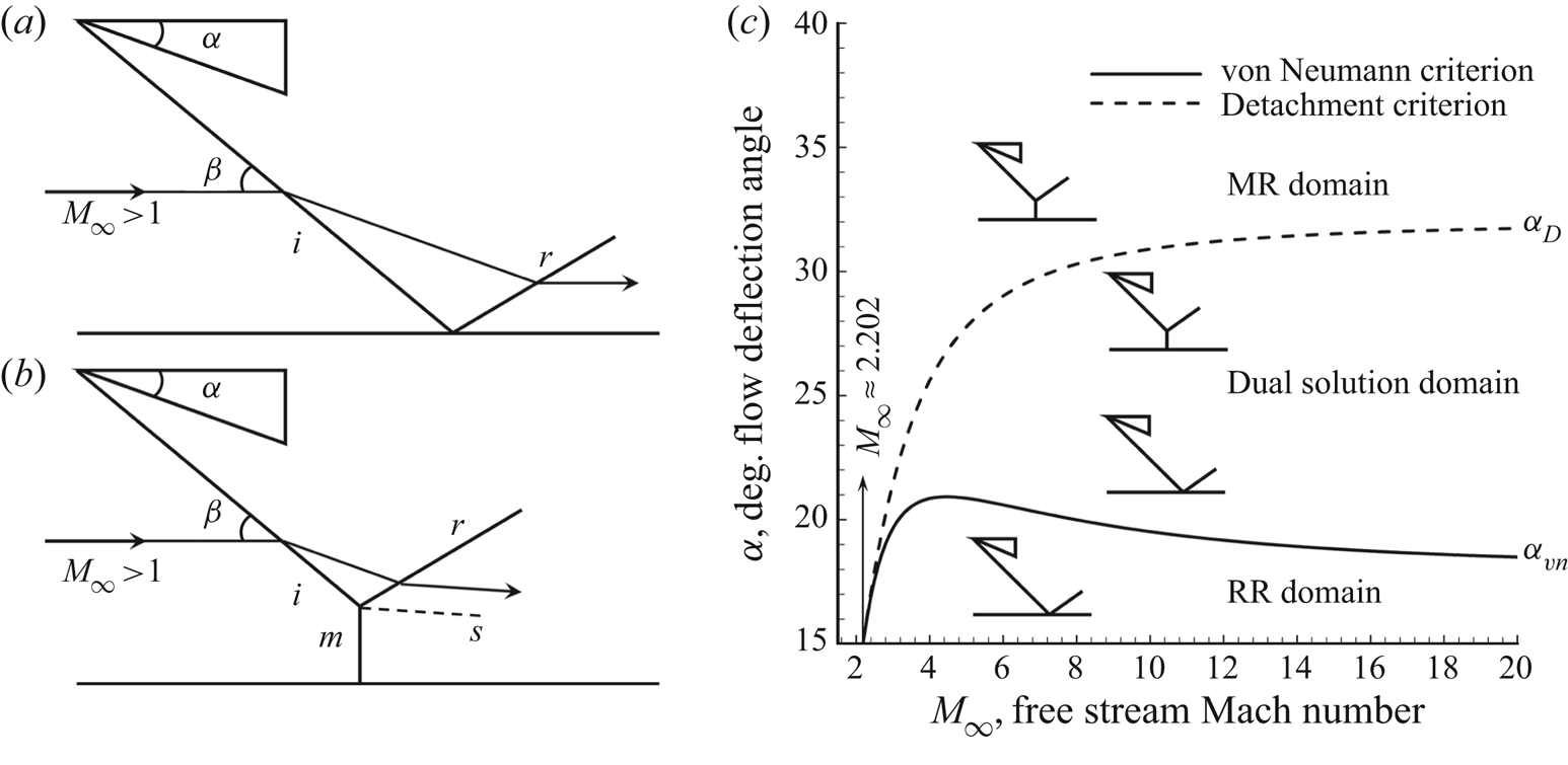
Shock reflections, including regular reflection (RR) and Mach reflection (MR), are fundamental phenomena existing widely in flow fields of supersonic as well as hypersonic vehicle bodies, inlets and nozzles. Analyses based on inviscid methods usually characterize the two flow configurations as sketches (see Tao, Fan & Zhao Reference Tao, Fan and Zhao2014) shown in figures 1(a) and 1(b). The former, RR configuration, consists of incident  $i$ and reflected
 $r$ shock waves, while the latter, MR, is shaped by an extra normal shock, knowing as Mach stem
 $m$. Additionally, because of the two different-velocity flows crossing, respectively,
 $r$ and
 $m$, downstream flow is separated by a slip line
 $s$. Theoretical solutions prove that reflection configurations rely on incoming Mach number
 $M_\infty$ and flow deflection angle
 $\alpha$, of which the relations are demonstrated by figure 1(c). Two classical criteria proposed by von Neumann (Reference von Neumann1943, Reference von Neumann1945), the von Neumann criterion (solid line,
 $\alpha _{vn}$) and the detachment criterion (dashed line,
 $\alpha _D$), divide the domain into three parts: RR domain with a small
 $\alpha$ below von Neumann criterion (
 $\alpha <\alpha _{vn}$); MR domain with a large
 $\alpha$ exceeding detachment criterion (
 $\alpha >\alpha _D$); and dual solution domain residing in the area between solid line and dashed line (
 $\alpha _{vn}<\alpha <\alpha _D$), in which both RR and MR are possible. Besides, the minimum valid Mach number for von Neumann criteria is
 $M_\infty \approx 2.202$.
Schematic illustration of inviscid shock reflection configurations and the domains of possible shock reflection pattern: (a) RR configuration, (b) MR configuration and (c) solution domains, based on the work of Tao et al. (Reference Tao, Fan and Zhao2014).

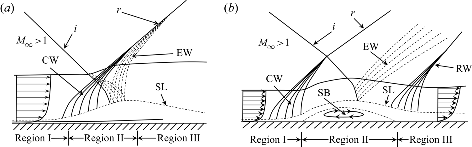
In fact, inviscid methods analyse flow characteristics incompletely, and the influence of boundary flow should be taken into consideration, which means the shock wave–boundary layer interaction (SWBLI) plays an important role in the shock reflection configurations (see D'elery & Bur Reference D'elery and Bur2000). The immersion of incident shock leads to a pressure rise in the boundary flow and results in an adverse pressure gradient on wall. This pressure disturbance propagates upstream via the subsonic channel and thickens the boundary layer, as shown in figure 2. If the pressure rise is not too large (figure 2a), in the interaction region (region II) close to the sonic line, both incident shock  $i$ and reflected shock
 $r$ are replaced by a series of weak waves including compression waves upstream and expansion waves downstream. When the pressure rise is large enough (figure 2b), boundary flow is separated by the formation of a separation bubble in region II. In the incipient interaction region (region I), compression waves grow higher out of the boundary layer and coalesce to form the separation shock
 $i_2$, which is reflected as shock
 $r_2$. Then the boundary flow reattaches in region III with the formation of a reattachment shock wave downstream.
Schematic illustration of oblique shock wave-turbulent boundary layer interactions: ( $a$) attached reflection and (
 $b$) separated reflection, based on the work of D'elery & Bur (Reference D'elery and Bur2000). CW, compression waves; EW, expansion waves; RW, reattachment shock wave; SL, sonic line; SB, separation bubble.

The pressure rise in the SWBLI region is determined by upstream and boundary flow properties, which could be well explained based on free interaction theory (FIT) (see Chapman, Kuehn & Larson Reference Chapman, Kuehn and Larson1958). According to FIT, the separation shock strength depends on Mach number and Reynolds number, while it shows independence with incident shock strength and downstream flow properties. For relatively strong shock waves, as shown in figure 2(b), the FIT could be well established (see D'elery & Marvin Reference D'elery and Marvin1986; Tao et al. Reference Tao, Fan and Zhao2014), while much less information is available in the literature for weak interactions, as shown in figure2(a), where a pressure plateau is never reached (see Giepman, Schrijer& van Oudheusden Reference Giepman, Schrijer and van Oudheusden2018).
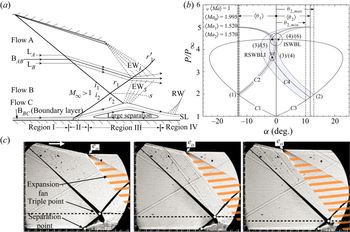
Several recent results from both computational fluid dynamics and experiments (see Matheis & Hickel Reference Matheis and Hickel2015; Giepman et al. Reference Giepman, Schrijer and van Oudheusden2018) prove that the separation bubble size grows almost linearly with the increase of incident shock strength, which could not be explained by FIT. Additionally, the experimental work conducted by Grossman & Bruce (Reference Grossman and Bruce2018) demonstrates a very strong influence of downstream flow on SWBLI, as shown in figure 3. Accordingly, only separation shock strength in region II (figure 3a) might be determined by boundary flow properties, while the majority of the separation shock seems to be dependent upon the separation bubble, which could be affected by downstream flow similar to the expansion fan (EW $_I$), as shown in figure3(c). This downstream influence could even intensify the separation shock strength of SWBLI in region III, and be strong enough to lead to transition of regular reflection to irregular reflection, as shown in figure3(b). Thus, the application of FIT is limited in some situations. On one hand the FIT might be only applicable up to the point of separation and responsible for some initial contributions to the separation shock; on the other hand the influence of incident shock strength as well as downstream flow disturbance on the configuration of SWBLI should not be neglected, indicating that there should be some other principles being applicable up to the situations with large separation.
Influence of expansion fan on shock wave–boundary layer interactions: ( $a$) schematic illustration of incident shock–separation shock interaction, (
 $b$) polar lines and (
 $c$) schlieren images with various expansion fans, based on the work of Grossman & Bruce (Reference Grossman and Bruce2018). ISWBLI, irregular reflection; RSWBLI, regular reflection.

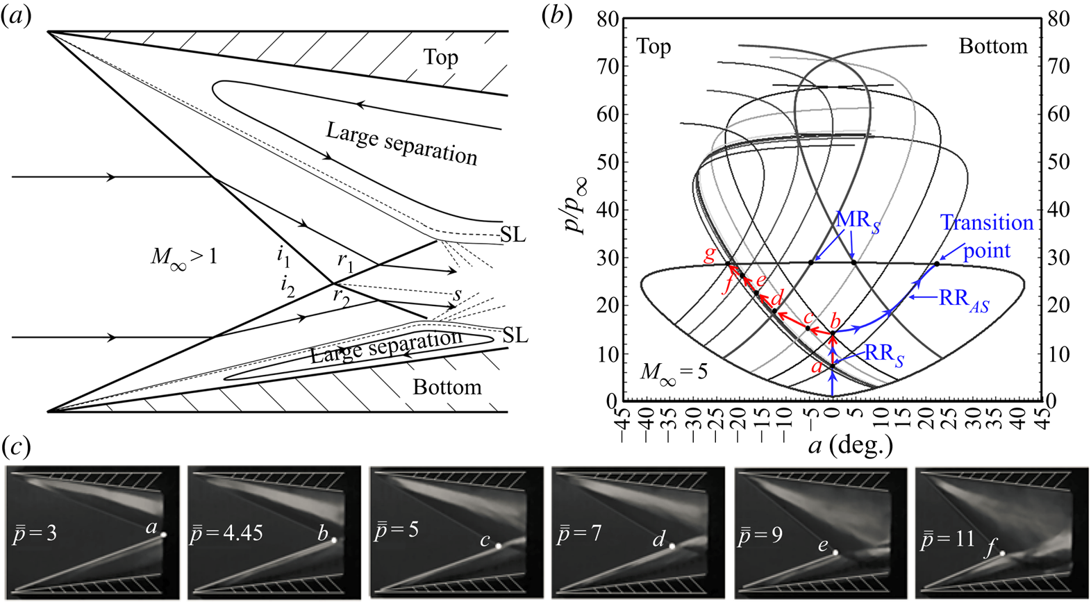
Some researchers attempt to explain the shock interaction principles from the view of entropy. Li & Ben-Dor (Reference Li and Ben-Dor1996a,Reference Li and Ben-Dorb) firstly employ the minimum entropy production principle (MEP) to propose new criteria for the RR–MR transition, which have been proved by experiments (see Chpoun et al. Reference Chpoun, Passerel, Li and Ben-Dor1995). Accordingly, in the work conducted by Wang et al. (Reference Wang, Xue and Cheng2018), MEP is employed to analyse the configurations as well as RR to MR transition of separation shock–separation shock interactions, as shown in figure 4, which agree well with experimental results. With both top and bottom boundary flow separated by a large separation region, as shown in figure 4(a), increasing downstream back pressure drives the separation shock–separation shock interaction solutions moving from point  $a$ to
 $g$, as shown in figures 4(b) and 4(c), indicating that downstream flow disturbance exerts a strong influence on separation shock strength, while effects of boundary flow properties are much weaker.
Influence of downstream back pressure on shock wave–boundary layer interactions: ( $a$) schematic illustration of separation shock–separation shock interaction, (
 $b$) solution path on shock polar lines changed by back pressure and (
 $c$) schlieren images with various downstream back pressures, based on the work of Wang, Xue & Cheng (Reference Wang, Xue and Cheng2018).

To sum up, according to the recent literature, in the situation with a relatively small separation bubble, boundary flow shows the dominant influence on SWBLI, while this influence becomes weaker with the separation bubble growing larger. The works mentioned above also demonstrate that separation shock seems to be curved, and the FIT could not predict well the separation shock strength in the situation with a relatively large separation region, applying to which should be other principles, while very little theoretical research into this situation exists. In addition, several studies prove that incident shock could affect SWBLI, but few of them could establish the connection between separation shock strength and the influences. Therefore, the motivation of the current study is to analyse the appearance of curved separation shock and establish the correlation between incident shock and separation shock. Aiming to solve these problems, theoretical methods including FIT and MEP focusing on the regular SWBLI are discussed in detail and, for verification, the current experiments are performed at Mach number 2 and 2.5 on test models with various wedge angles of  $9^\circ$,
 $12^\circ$,
 $13^\circ$,
 $15^\circ$,
 $17^\circ$,
 $19^\circ$,
 $20^\circ$ and
 $21^\circ$.
2. Theoretical methods and analyses
2.1. Free interaction theory and the minimum entropy production principle
The free interaction theory is proposed firstly by Chapman et al. (Reference Chapman, Kuehn and Larson1958), according to which the pressure rise  $p_{\textit{FIT}}/p_\infty$ in the separation region as shown in figure 2(b) can be expressed as follows:
 \begin{equation} \frac{p_{\textit{FIT}}}{p_\infty}=1+F(\bar{x}){\gamma}{M_\infty}^2\sqrt{\frac{C_{f0}}{2({M_\infty}^2-1)^{0.5}}}, \end{equation}
herein  $\gamma$ is the specific heat ratio and
 $F(\bar {x})$ is a universal correlation function which depends on pressure rise distance and flow patterns. In turbulent flow,
 $F(\bar {x})$ is proposed by Erdos & Pallone (Reference Erdos and Pallone1962) such that
 $F(\bar {x})_{tur0}\approx 4.22$ close to separation point and
 $F(\bar {x})_{tur1}\approx 6$ for pressure plateau, while in laminar flow,
 $F(\bar {x})$ is found experimentally such that
 $F(\bar {x})_{lam0}\approx 0.8$ and
 $F(\bar {x})_{lam1}\approx 1.5$, respectively (see Hakkinen et al. Reference Hakkinen, Greber, Trilling and Abarbanel1959; Babinsky & Harvey Reference Babinsky and Harvey2011). Here,
 $C_{f0}$ is skin friction coefficient, which could be obtained according to incoming flow conditions (see Tao et al. Reference Tao, Fan and Zhao2014). Therefore, the independent variables of FIT are upstream flow properties including free stream Mach number
 $M_\infty$ and skin friction coefficient
 $C_{f0}$.
The minimum entropy production principle is employed firstly by Li & Ben-Dor (Reference Li and Ben-Dor1996a,Reference Li and Ben-Dorb) to determine the criteria of RR to MR transition in steady as well as unsteady shock–shock interaction flow, based on which the MEP is employed to analyse the separation shock–separation shock interactions by Wang et al. (Reference Wang, Xue and Cheng2018). In the flow shown in figure 4(a), an implicit function is derived to establish the connection among the configuration of separation shock–separation shock interaction, total entropy production and flow conditions, which is expressed as follows:
 \begin{equation} \ddot{S}_{RR}=f_{SRR}(M_\infty,\beta_i,\bar{\bar{p}}), \end{equation}
where total entropy production factor  $\ddot {S}_{RR}$ is related to variables of the incoming Mach number
 $M_\infty$, separation shock angle
 $\beta _i$ and equivalent back pressure
 $\bar {\bar {p}}$. The implicit relation of (2.2) is determined by the expressions of
 $\ddot {S}_{RR}$ and
 $\bar {\bar {p}}$.
Here,  $\ddot {S}_{RR}$ is derived by employing the incoming mass flow rate (two-dimensional flow) to normalize total entropy production
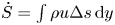 $\dot {S}=\int \rho u{\rm \Delta} s \,\textrm {d}y$ (see Li & Ben-Dor Reference Li and Ben-Dor1996a; Wang et al. Reference Wang, Xue and Cheng2018)
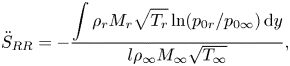 \begin{equation} \ddot{S}_{RR}=-\frac{\displaystyle\int\rho_rM_r\sqrt{T_r}\ln(p_{0r}/p_{0\infty})\,\textrm{d}y}{l\rho_\infty M_\infty \sqrt{T_\infty}}, \end{equation}
where  $\rho$,
 $M$,
 $T$,
 $p_0$ and
 $l$ denote the local density, Mach number, static temperature, total pressure and the height of incoming flow, respectively. The subscripts
 $\infty$ and
 $r$ denote far-field flow and flow crossing downstream reflected shock waves, respectively.
Here  $\bar {\bar {p}}$ is expressed as follows:
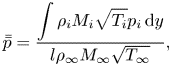 \begin{equation} \bar{\bar{p}}=\frac{\displaystyle\int\rho_iM_i\sqrt{T_i}p_i\,\textrm{d}y}{l\rho_\infty M_\infty \sqrt{T_\infty}}, \end{equation}
where subscript  $i$ denotes flow crossing upstream incident (or separation) shock waves. According to the work of Wang et al. (Reference Wang, Xue and Cheng2018), the influence of downstream pressure disturbance on shock–shock interaction could be measured by
 $\bar {\bar {p}}$. Because the variables can be obtained by incoming Mach number
 $M_\infty$ and local shock angle
 $\beta _i$, for shock
 $i_1$–shock
 $i_2$ interaction flow shown in figure 4(a), (2.3) and (2.4) can be written as
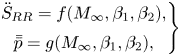 \begin{equation} \left.\begin{array}{@{}c@{}} \ddot{S}_{RR}=f(M_\infty,\beta_1,\beta_2),\\ \bar{\bar{p}}=g(M_\infty,\beta_1,\beta_2), \end{array} \right\} \end{equation}
herein  $\beta _1$ and
 $\beta _2$ are shock angles of
 $i_1$ and
 $i_2$, respectively. Then (2.2) is derived by inserting
 $\beta _1=g^{-1}(M_\infty ,\beta _2,\bar {\bar {p}})$ into
 $f(M_\infty ,\beta _1,\beta _2)$. According to the MEP, for given flow conditions (neglect heat exchange), if
 $f_{SRR}(M_\infty ,\beta _2,\bar {\bar {p}})=\min$, (2.2) should fulfil the following limitations:
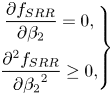 \begin{equation} \left.\begin{array}{@{}c@{}} \displaystyle\dfrac{\partial f_{SRR}}{\partial \beta_2}=0,\\ \displaystyle\dfrac{\partial^2 f_{SRR}}{\partial {\beta_2}^2}\geq0, \end{array} \right\} \end{equation}
thus, for the flow fields shown in figure 4(a) with a given incoming Mach number, the correlation between separation shock strength and downstream pressure disturbance are determined, of which the theoretical solution path validated by experimental results is shown in figures 4(b) and 4(c).
Obviously, the two theoretical methods apply to interaction flow in different situations. On one hand, the FIT method attributes the separation shock strength only to boundary layer, indicating it could apply well to upstream portion of separation shock; on the other hand, the MEP method concentrates on the spatial structure of shock–shock interaction, which applies well to the downstream portion of separation shock with relatively large separation.
2.2. Proposed method for analysing regular SWBLI
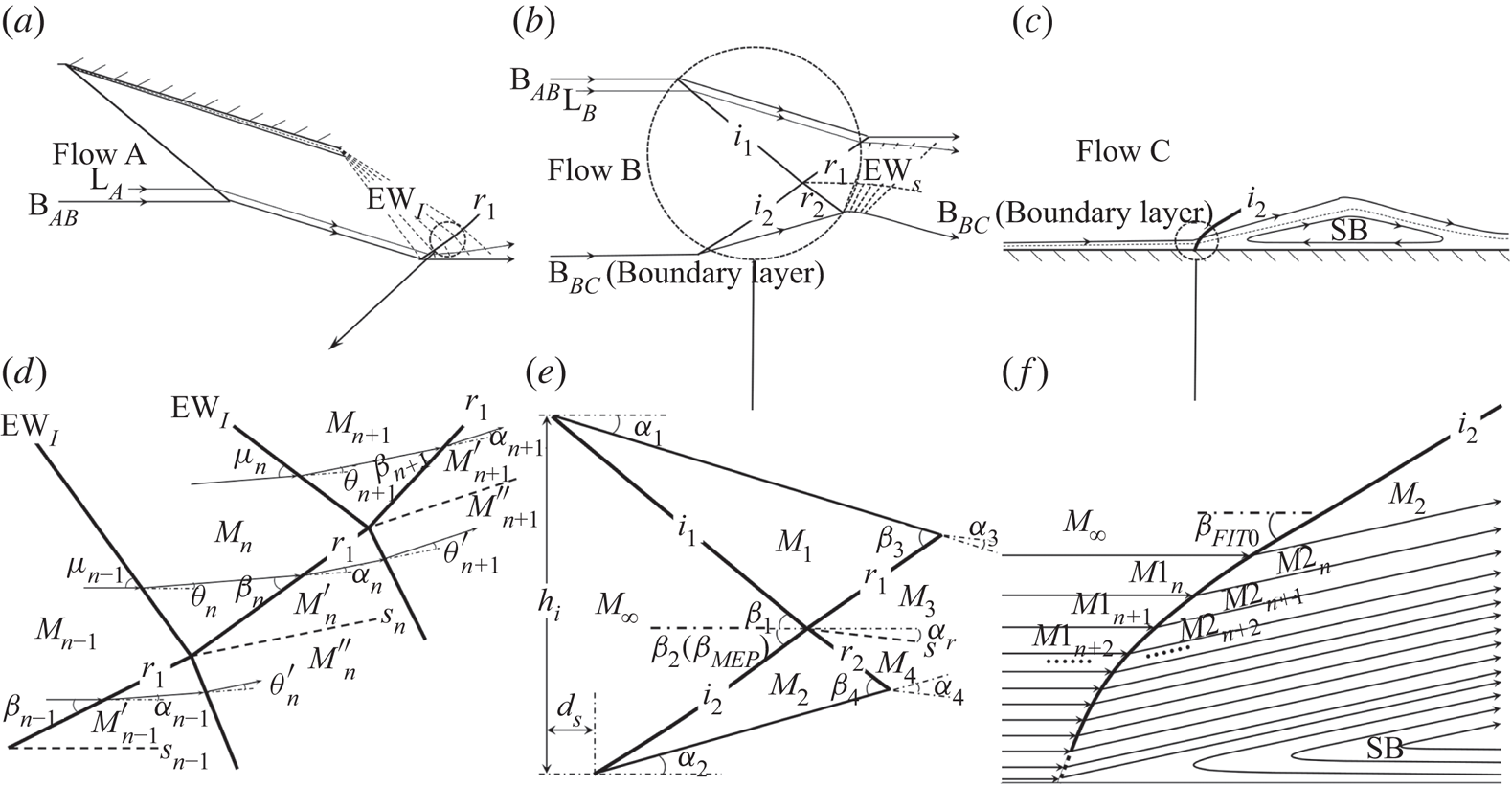
Because the configurations of SWBLI might be affected by many factors including boundary layer (see Matheis & Hickel Reference Matheis and Hickel2015), incident shock strength (see Giepman et al. Reference Giepman, Schrijer and van Oudheusden2018) and downstream expansion fan (see Grossman & Bruce Reference Grossman and Bruce2018), the flow fields shown in figure 3(a) can be classified into such three flow components shown in figure5( $a$–
 $c$): flow A of the wedge-induced flow, which is mainly determined by wedge angle and downstream expansion waves; flow B of the main interaction flow, which is related to incident shock and separation shock; flow C of the boundary layer flow and separation bubble, which can be affected by viscosity and skin friction. Here, B
 $_{AB}$ and B
 $_{BC}$ denote the boundaries between flow A and B and flow B and C, respectively. Streamlines in flow B (L
 $_B$) show weak effects of downstream flow, and reflected shock
 $r_1$ in this flow field is consequently straight and relatively strong, as shown in figure5(
 $e$). However, in flow A, streamlines L
 $_A$ bend upward (or downward) because of expansion waves EW
 $_I$ (or EW
 $_S$), leading to a curved reflected shock
 $r_1$ in this flow field, as shown in figure 5(
 $d$). It might be noticed that flow A is similar with inviscid flow, flow B can be assumed as an overall shock–shock interaction flow, and flow C mostly depends on boundary flow.
Schematic illustration of classification for flows in SWBLI: ( $a$) wedge induced flow; (
 $b$) main interaction flow; (
 $c$) boundary layer flow; (
 $d$) detailed flow A, reflected shock–expansion waves interaction; (
 $e$) detailed flow B, incident shock–separation shock interaction; and (
 $\,f$) detailed flow C, boundary layer-separation shock interaction.
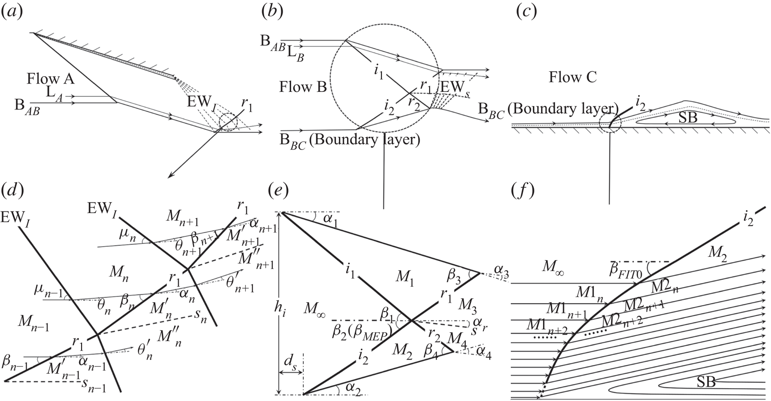
The configuration of flow A is mainly characterized by shock–expansion waves interaction, as shown in figure 5( $d$), in which the reflected shock
 $r_1$ could be computed in steps via assuming the expansion fan as a series of weak waves, e.g. the total flow deflection angle
 $\theta$ is replaced by finite small angles
 $\theta _n$ (the number is
 $\theta /\theta _n$). When each flow deflection angle
 $\theta _n$ is small enough, pressure rise
 $p_n/p_{n-1}$ and Mach number
 $M_n$ of flow crossing n waves could be obtained by the second-order approximate solution derived as follows:
 \begin{gather} \frac{p_n}{p_{n-1}}=1-\frac{\gamma {M_{n-1}}^2\theta_n}{\sqrt{{M_{n-1}}^2-1}}+\frac{\gamma {M_{n-1}}^2{\theta_n}^2[(\gamma+1){M_{n-1}}^4-4({M_{n-1}}^2-1)]}{4({M_{n-1}}^2-1)^2}, \end{gather}
 \begin{gather} M_n=\sqrt{\frac{2}{\gamma-1}\left[\left(1+\frac{\gamma-1}{2}{M_{n-1}}^2\right)\left(\frac{p_n}{p_{n-1}}\right)^{({1-\gamma})/{\gamma}}-1\right]}. \end{gather}
The local pressure rise  $p'_n/p_n$, shock angle
 $\beta _n$ and flow deflection angle
 $\alpha _n$ of flow crossing
 $r_1$ can be expressed by following:
 \begin{gather} \frac{p'_n}{p_n}=\frac{2\gamma}{\gamma+1}{M_n}^2\sin^2\beta_n-\frac{\gamma-1}{\gamma+1}, \end{gather}
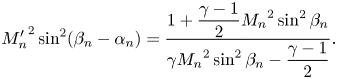 \begin{gather} {M'_n}^2\sin^2(\beta_n-\alpha_n)=\frac{1+\dfrac{\gamma-1}{2}{M_n}^2\sin^2\beta_n}{\gamma {M_n}^2\sin^2\beta_n-\dfrac{\gamma-1}{2}}. \end{gather}
In addition, the pressure rise and flow deflection angles should be the same on both sides of slip line  $s_n$
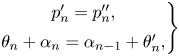 \begin{equation} \left. \begin{array}{@{}c@{}} p'_n=p''_n,\\ \theta_n+\alpha_n=\alpha_{n-1}+\theta'_n, \end{array} \right\} \end{equation}
herein  $p''_n$ could be obtained by (2.7) with
 $M'_{n-1}$ and
 $\theta '_n$, and
 $M'_{n-1}$ could be obtained by (2.10) with
 $M_{n-1}$,
 $\alpha _{n-1}$ and
 $\beta _{n-1}$. The equations are closed and then all the variables are determined in steps based on the incoming flow conditions.
Flow B is an incident shock–separation shock interaction. As shown in figure 5( $e$), the main entropy is produced by all the incident and reflected shock waves, hence (2.3) could be written as
 \begin{equation} \ddot{S}_{RR}=-\frac{\displaystyle\int\rho_3M_3\sqrt{T_3}\ln(p_{03}/p_{0\infty})\,\textrm{d}y+\int\rho_4M_4\sqrt{T_4}\ln(p_{04}/p_{0\infty})\,\textrm{d}y}{l\rho_\infty M_\infty \sqrt{T_\infty}}.\end{equation}
Assume that all the shock waves  $i_1$,
 $i_2$,
 $r_1$ and
 $r_2$ are straight and the local flow fields behind the shock waves are uniform, then (2.12) could be derived as
 \begin{align} \displaystyle\ddot{S}_{RR}&=-\frac{1}{\rho_\infty M_\infty \sqrt{T_\infty}} \left[k_{i1}\rho_1M_1\sqrt{T_1}\ln\left(\frac{p_{01}}{p_{0\infty}}\right)+ k_{i2}\rho_2M_2\sqrt{T_2}\ln\left(\frac{p_{02}}{p_{0\infty}}\right)\right.\nonumber\\ &\left.\quad +k_{r1}\rho_3M_3\sqrt{T_3}\ln\left(\frac{p_{03}}{p_{01}}\right)+ k_{r2}\rho_4M_4\sqrt{T_4}\ln\left(\frac{p_{04}}{p_{02}}\right)\right], \end{align}
herein the coefficients  $k_{i1}$,
 $k_{i2}$,
 $k_{r1}$ and
 $k_{r2}$ are derived as follows:
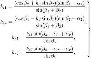 \begin{equation} \left.\begin{array}{@{}c@{}} \displaystyle k_{i1}=\dfrac{(\cos\beta_2+k_d\sin\beta_2)(\sin\beta_1-\alpha_1)}{\sin(\beta_1+\beta_2)},\\ \displaystyle k_{i2}=\dfrac{(\cos\beta_1-k_d\sin\beta_1)(\sin\beta_2-\alpha_2)}{\sin(\beta_1+\beta_2)},\\ \displaystyle k_{r1}=\dfrac{k_{i1}\sin(\beta_3-\alpha_1+\alpha_r)}{\sin\beta_3},\\ \displaystyle k_{r2}=\dfrac{k_{i2}\sin(\beta_4-\alpha_2-\alpha_r)}{\sin\beta_4}, \end{array} \right\} \end{equation}
where  $k_d$ is a non-dimensional variable to denote the local position of the separation point, i.e.
 $k_d=d_s/h_i$, as shown in figure 5(
 $e$). Here,
 $\alpha _r$ is the flow deflection angle on both sides of the slip line according to the solution of regular reflection with incident shock waves. Here, (2.4) should be written as
 \begin{equation} \bar{\bar{p}}=\frac{p_1\rho_1M_1\sqrt{T_1}k_{i1}+p_2\rho_2M_2\sqrt{T_2}k_{i2}}{\rho_\infty M_\infty \sqrt{T_\infty}}. \end{equation}
In addition, reflected shock angles,  $\beta _3$ and
 $\beta _4$, are determined by incoming Mach number
 $M_\infty$ and incident shock angles
 $\beta _1$ and
 $\beta _2$. Thus
 $\beta _2$ depends on
 $M_\infty$,
 $\beta _1$ and
 $\bar {\bar {p}}$ under the limitations of (2.6). Then
 $\beta _2$ could be obtained from the implicit functions by iterative solution methods. Herein
 $\bar {\bar {p}}$ represents downstream disturbance exerted on interaction, of which the lower bound corresponds to ideal flow conditions without any disturbance (see Wang et al. Reference Wang, Xue and Cheng2018).
Flow C is boundary flow, in which the pressure rise  $p_{\textit{FIT}}/p_\infty$ is obtained by (2.1) with given
 $M_\infty$ and
 $C_{f0}$ based on the FIT method. Then separation shock angle
 $\beta _{\textit{FIT}}$ (
 $\beta _{\textit {FIT}0}$ or
 $\beta _{\textit {FIT}1}$) could be computed by following:
 \begin{equation} \beta_{\textit{FIT}}=\arcsin\left[\left(\frac{p_{\textit{FIT}}}{p_\infty}+\frac{\gamma-1}{\gamma+1}\right) \frac{\gamma+1}{2\gamma{M_\infty}^2}\right]^{0.5}. \end{equation}
It should be noted that  $M_\infty$ should be replaced by
 $M_{1n}$ inside of the boundary layer as shown in figure 5(
 $\,f$), which means the separation shock bends downward because of the lower Mach number.
3. Results and discussions
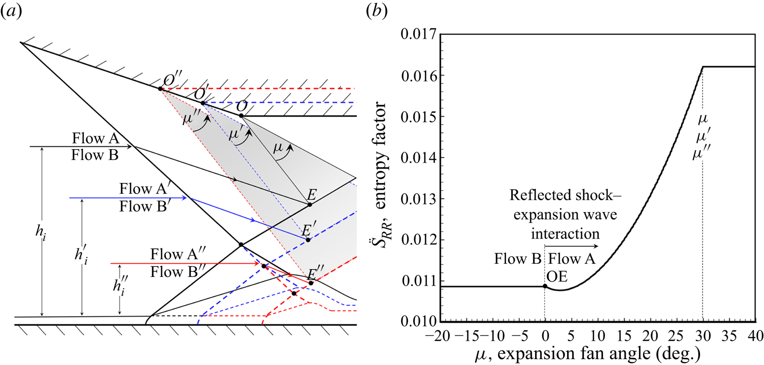
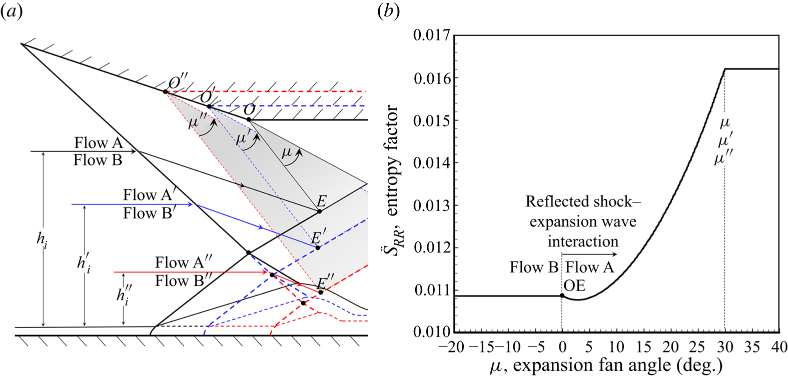
The flow B is formed by flow self-adjusting to a configuration that fulfils the minimum entropy production, as shown in figure 6( $a$), which means the downstream expansion fan affects SWBLI by changing the width of flow B. The evidence could be observed from the work of Grossman & Bruce (Reference Grossman and Bruce2018), who conducted experiments on
 $12^\circ$ wedge models with various expansion wave positions in Mach number 2 flow, as shown in figure 3(
 $c$), based on which the local entropy factor of flow crossing reflected shock–expansion wave interaction is shown in figure 6(
 $b$). The entropy factor line demonstrates that expansion waves could increase the local entropy production, when reflected shock–expansion wave interaction gets closer to incident shock–separation shock interaction, the flow B would be suppressed and adjusted to a new configuration with a smaller
 $h_i$, as shown in figure6(
 $a$). It should be noticed that, the initial separation shock strength close to the boundary layer is mostly determined by the FIT method, which means the FIT solution and the MEP solution interfere with each other if the expansion fan gets close enough to SWBLI.
Influence of expansion fan on SWBLI and entropy factor: ( $a$) sketch of SWBLI changed by expansion fan and (
 $b$) local entropy factor of reflected shock–expansion wave interaction at
 $M_\infty =2$,
 $\alpha _1=12^\circ$.
Assume that analytical solutions of both FIT and MEP methods are computed under ideal conditions without any disturbances, respectively. Then the FIT solution is only related to incoming Mach number  $M_\infty$ and skin friction coefficient
 $C_{f0}$, while the MEP solution depends on
 $M_\infty$ and incident flow deflection angle
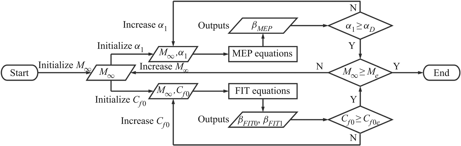
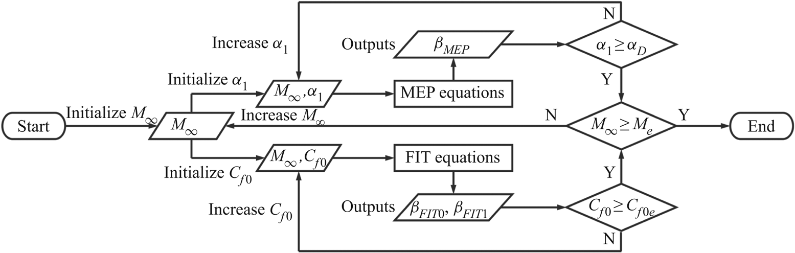
 $\alpha _1$. The combined method for solving separation shock angle is summarized in figure 7 (
 $\alpha _D$ represents detachment condition,
 $M_e$ and
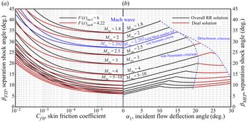
 $C_{f0e}$ are given conditions representing the ranges of inputs and outputs), of which the results in turbulent flow are illustrated in figure 8.
Flow chart of solving separation shock angle based on combined method (FIT and MEP).
Analytical solutions of separation shock angle based on different theoretical methods: ( $a$) FIT method for turbulent boundary flow and (
 $b$) MEP method for shock–shock interaction flow.
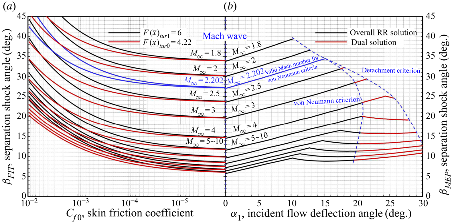
In figure8( $a$), the shock angle in relatively upstream flow close to the boundary layer, denoted as
 $\beta _{\textit {FIT}0}$, and the shock angle on pressure plateau, denoted as
 $\beta _{\textit {FIT}1}$, are computed by setting
 $F(\bar {x})_{tur0}=4.22$ and
 $F(\bar {x})_{tur1}=6$, respectively, where both separation shock solutions show tendencies toward Mach waves with much lower
 $C_{f0}$. While in figure8(
 $b$), incident shock plays an important role in shock–shock interaction, where three boundary lines (dashed lines) divide the solution domain, denoted as
 $\beta _{\textit {MEP}}$, into three parts. The first line, Mach wave line, represents the lower bound, followed by very weak incident and separation shock waves growing in different latitudes. The second and third lines are the von Neumann criterion and detachment criterion, respectively, between which both regular reflection and Mach reflection are possible. Additionally, figure8(
 $b$) demonstrates that the growth of MEP solution lines seems to be slower in hypersonic flow (
 $M_\infty >5$). It could consequently be indicated that unseparated flow is more likely to exist in the situations of lower skin friction coefficients (figure 8
 $a$), weaker incident shock waves (figure 8
 $b$) and higher incoming Mach numbers (figure 8
 $b$). Normally, theoretical solutions based on FIT and MEP might be different under the same conditions. The most plausible explanation is, on one hand, both of the two theoretical results are obtained under ideal conditions without any disturbances; on the other hand, the FIT solution contributes to the initial pressure rise, while the MEP solution could be in charge of the downstream separation shock strength close to the shock–shock interaction point, which is similar to the viewpoint concluded by Grossman & Bruce (Reference Grossman and Bruce2018). Free interaction might only exist in relatively upstream separation regions while it would not be ‘free’ but suppressed by shock–shock interaction points. Assume that
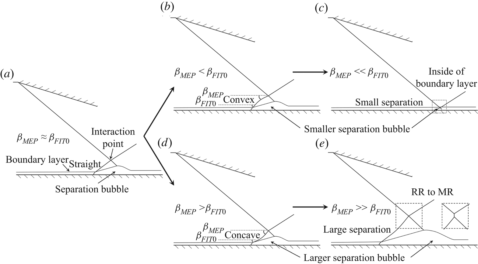
 $\beta _{\textit {MEP}}\approx \beta _{\textit {FIT}0}$ as shown in figure 9(
 $a$); the separation shock is approximately straight, while the differentiation of the two solutions leads to a curved separation shock due to different theoretical results on different portions, the shock angle is therefore transited from one solution to the other, resulting in several possible flow patterns as shown in figure 9(
 $b$–
 $e$).
Theoretical results of possible configurations for SWBLI: ( $a$)
 $\beta _{\textit {MEP}}\approx \beta _{\textit {FIT}0}$, (
 $b$)
 $\beta _{\textit {MEP}}<\beta _{\textit {FIT}0}$, (
 $c$)
 $\beta _{\textit {MEP}}\ll \beta _{\textit {FIT}0}$, (
 $d$)
 $\beta _{\textit {MEP}}>\beta _{\textit {FIT}0}$ and (
 $e$)
 $\beta _{\textit {MEP}}\gg \beta _{\textit {FIT}0}$.
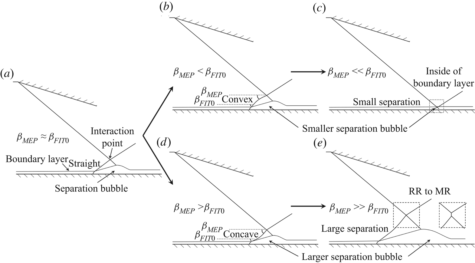
If  $\beta _{\textit {MEP}}<\beta _{\textit {FIT}0}$ as shown in figure 9(
 $b$), the separation shock needs to transit from a large angle to a small one, resulting in a convex shock. The pressure plateau is therefore replaced by a lower pressure, which means the separation bubble needs to become smaller to fit a lower pressure rise. In addition, when
 $\beta _{\textit {MEP}}$ is much weaker than
 $\beta _{\textit {FIT}0}$, the separation bubble should be much smaller, reducing the height of the interaction point, which might be inside of the boundary layer, as shown in figure 9(
 $c$). This configuration corresponds to relatively weak incident shock waves, and it can explain the work conducted on small angle wedges by Giepman et al. (Reference Giepman, Schrijer and van Oudheusden2018), who found the pressure plateau could not reach the FIT pressure rise.
On the contrary, if  $\beta _{\textit {MEP}}>\beta _{\textit {FIT}0}$ as shown in figure 9(
 $d$), the separation shock is a concave one with a larger separation bubble. This flow pattern can explain the work conducted on various angles of incident shock waves by Matheis & Hickel (Reference Matheis and Hickel2015) and Giepman et al. (Reference Giepman, Schrijer and van Oudheusden2018), in which the separation bubble size was observed growing almost linearly with the increase of incident shock strength. When
 $\beta _{\textit {MEP}}$ is much stronger than
 $\beta _{\textit {FIT}0}$ with a long concave separation shock, as shown in figure 9(
 $e$), the Mach interaction is more likely to exist. This configuration corresponds to large incident shock angles, and it can explain the work conducted on relatively large angle wedges by Grossman & Bruce (Reference Grossman and Bruce2018), who observed both regular and Mach interactions on a same test model, finding that the pressure plateau is higher than the FIT pressure rise, and assumed that the separation shock might be a curved shock.
4. Experiments and verification
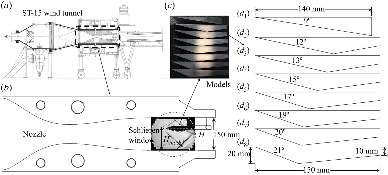
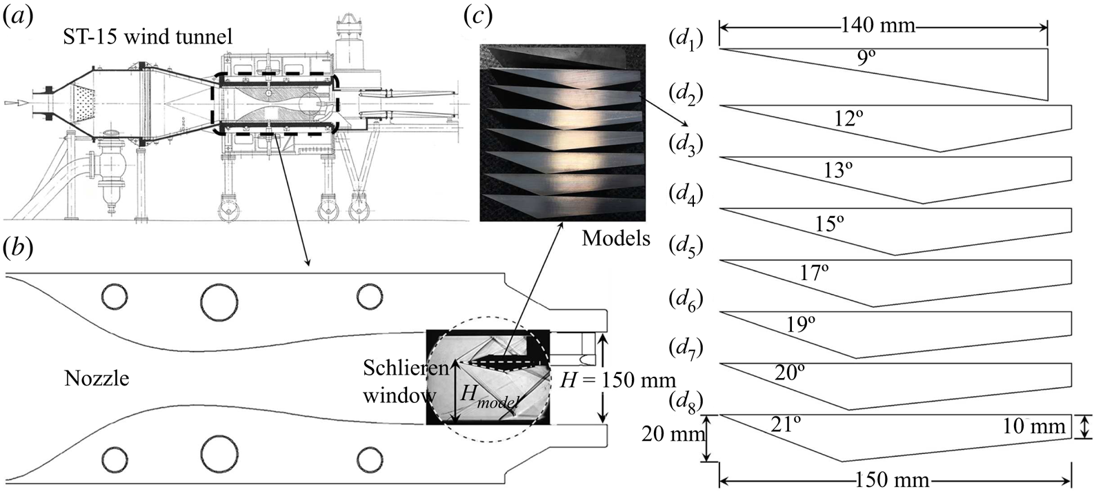
To validate theoretical results, the current experiments were performed in the ST-15 supersonic wind tunnel employing a schlieren system at Delft University of Technology. As shown in figure 10( $a$), ST-15 is a blowdown wind tunnel with a
 $150\ \textrm {mm}\times 150\ \textrm {mm}$ test section (figure 10
 $b$), which can perform various free steam Mach numbers of
 $M_\infty =1.5$, 2.0, 2.5 and 3.0 by alternative nozzles, and both the
 $M_\infty =2.0$ and 2.5 nozzles were employed for current study. In the optical path of a schlieren system, as shown in figure10(
 $b$), the flow configurations were captured via a 200 mm-diameter circular window by a high speed camera, which operated at a frame rate of 5 kHz with a 2 s sampling time and a resolution of
 $2016\times 2016$ pixels. The knife edge for schlieren images is vertical. The test model, shown in figure 10(
 $c$), mounted in the test section, is also alternative, of which the wedge angles are
 $9^\circ$,
 $12^\circ$,
 $13^\circ$,
 $15^\circ$,
 $17^\circ$,
 $19^\circ$,
 $20^\circ$ and
 $21^\circ$, as shown in figure 10(
 $d_1$–
 $d_8$), respectively. The model with the
 $9^\circ$ wedge is 140 mm long and 120 mm wide, while the others are 150 mm in length, 120 mm in width, 20 mm in maximum thickness and 10 mm in the most downstream thickness.
Schematic illustration of ST-15 wind tunnel and test models: ( $a$) ST-15 wind tunnel, (
 $b$) test section, (
 $c$) test models and (
 $d_1$)–(
 $d_8$) are major sizes of models, respectively.
4.1. Influence of the MEP solution on SWBLI
A non-dimensional parameter  $AR_{eff}$ defined by Grossman & Bruce (Reference Grossman and Bruce2018) is employed to measure the effect of the test section width divided by the height of the model upstream leading edge. The downstream expansion fan, which was observed by Grossman & Bruce (Reference Grossman and Bruce2018) shown in figure 3, could exert a strong influence on SWBLI with
 $AR_{eff}=1.0$. Therefore, in order to research the effect of the MEP solution on SWBLI, the models with various angles are mounted at
 $AR_{eff}=1.50$ in the Mach number
 $M_\infty =2.5$ tests to weaken the effect of downstream expansion fan, of which the incoming total pressure and total temperature are set as
 $P_0=3.0$ bar and
 $T_0=285$ K, respectively.
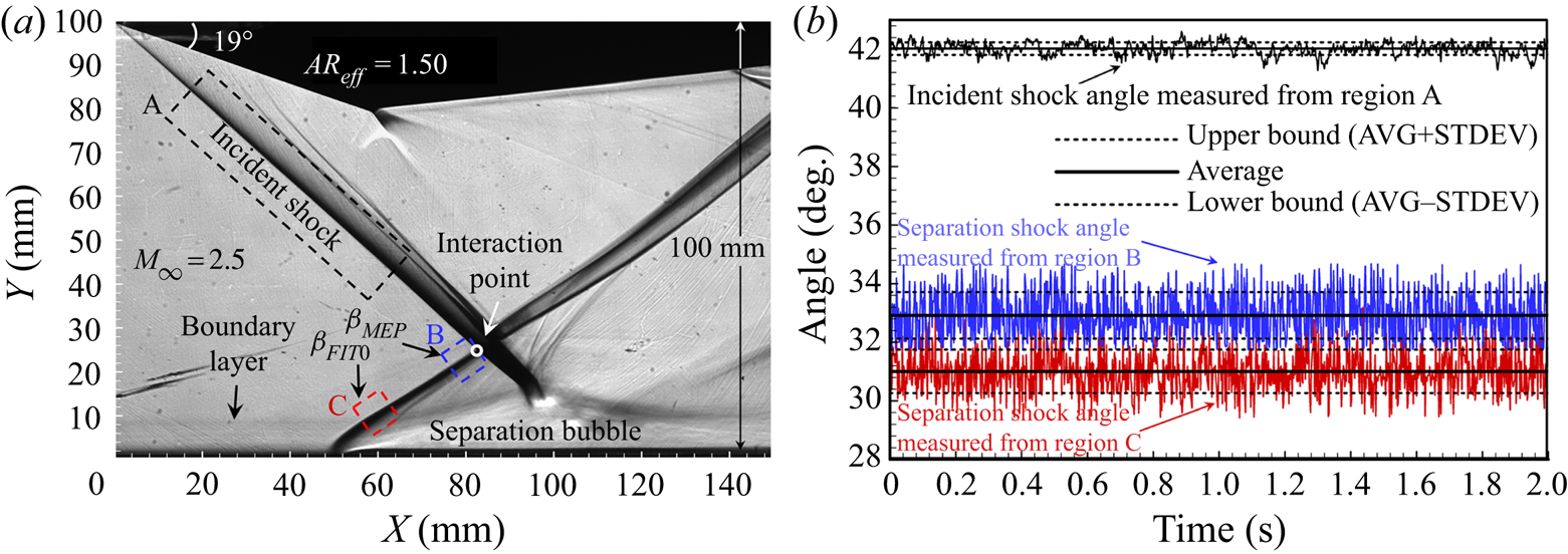
Because of the three-dimensional interference on both sides of the wedge accompanied by a series of Mach waves, both the incident and separation shock waves close to the interaction point are very thick, as shown in figure 11( $a$), resulting in the uncertainty of shock angle measurement. In the similar work of Grossman & Bruce (Reference Grossman and Bruce2018), who employed surface oil flow visualization to show separation region topology on the wind tunnel floor, the most upstream separation line was observed approximately straight while the three-dimensional flow effect seemed to be stronger in relatively downstream region. Therefore, the relatively upstream flow in the current study could be assumed as two-dimensional, and the upstream edge of shock line in schlieren image is consequently used for shock angle measurement. Additionally, although the separation points experience different positions, the influence of thickness change of boundary layer on SWBLI is small enough to be neglected, according to Grossman & Bruce (Reference Grossman and Bruce2018). An algorithm program for schlieren image quantization based on grey level (see Xue, Wang & Cheng Reference Xue, Wang and Cheng2018) is employed to detect the shock angles, by which the time history lines of incident shock angle on region A, separation shock angle close to interaction point on region B and separation shock angle close to boundary layer on region C were detected and illustrated in figure 11(
 $b$). In the following sections, the average value (
 $AVG$) of angles is used for interaction analyses on shock polar lines, and the error bars are characterized by standard deviation (STDEV ) such that
 $\mathit {Upper bound}=\mathit {AVG}+\mathit {STDEV}$ and
 $\mathit {Lower bound}=\mathit {AVG}-\mathit {STDEV}$.
Example of experimental result on the  $19^\circ$ wedge model in
 $M_\infty =2.5$ flow: (
 $a$) schlieren image and (
 $b$) measured shock angles by program algorithm.
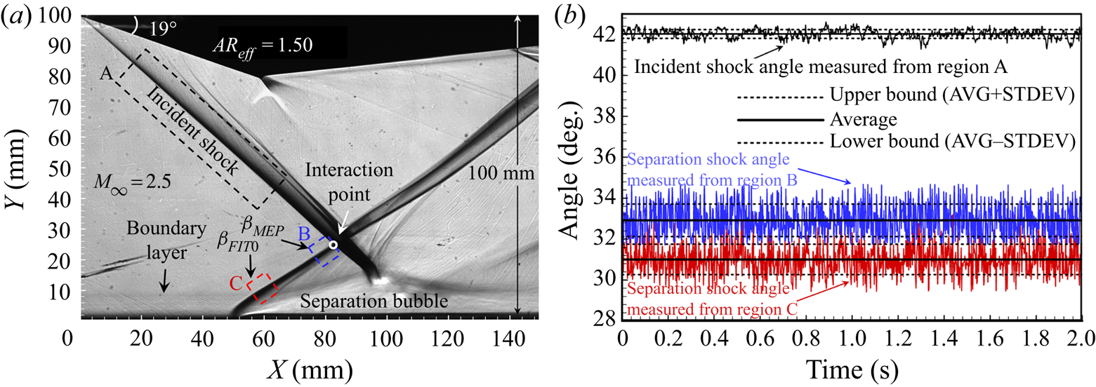
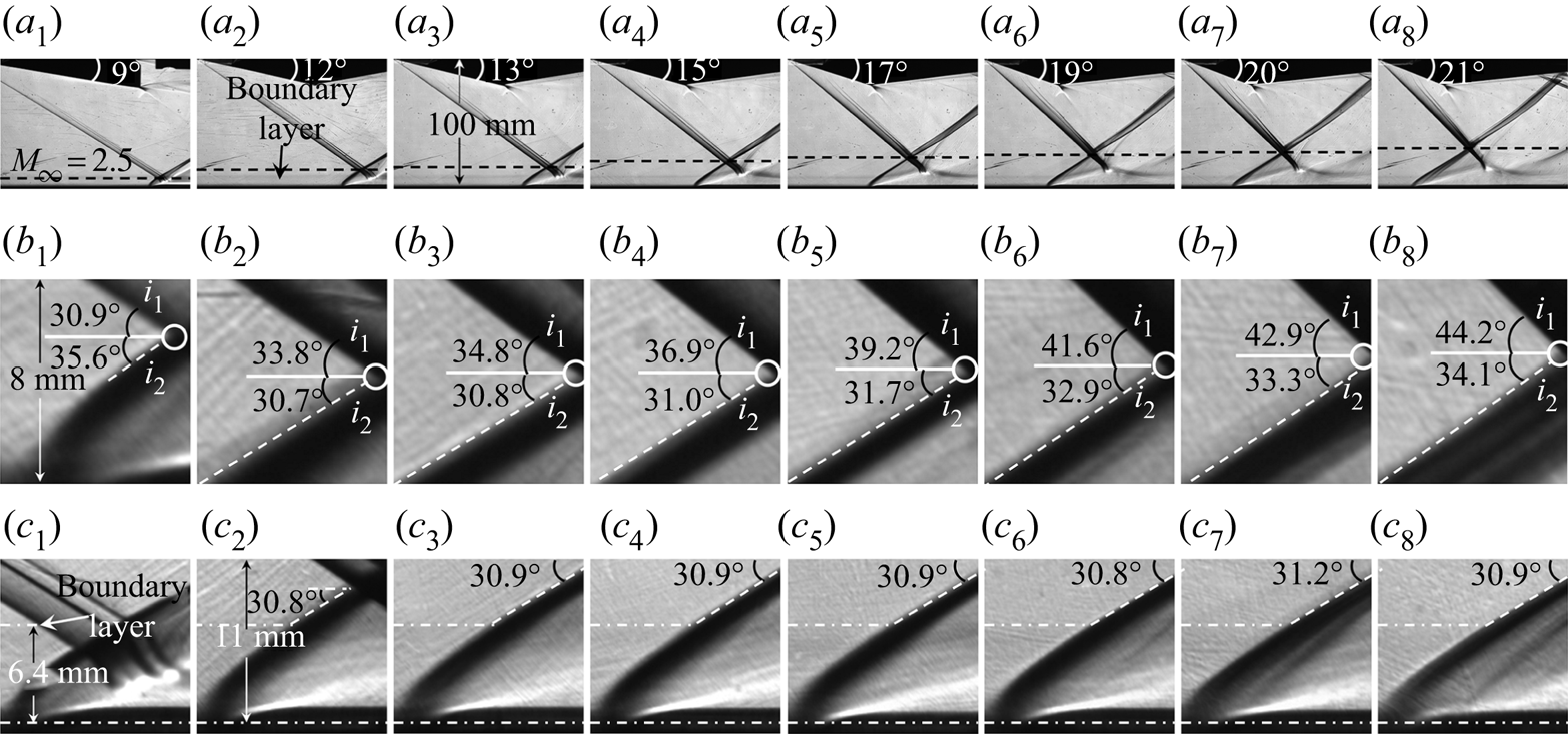
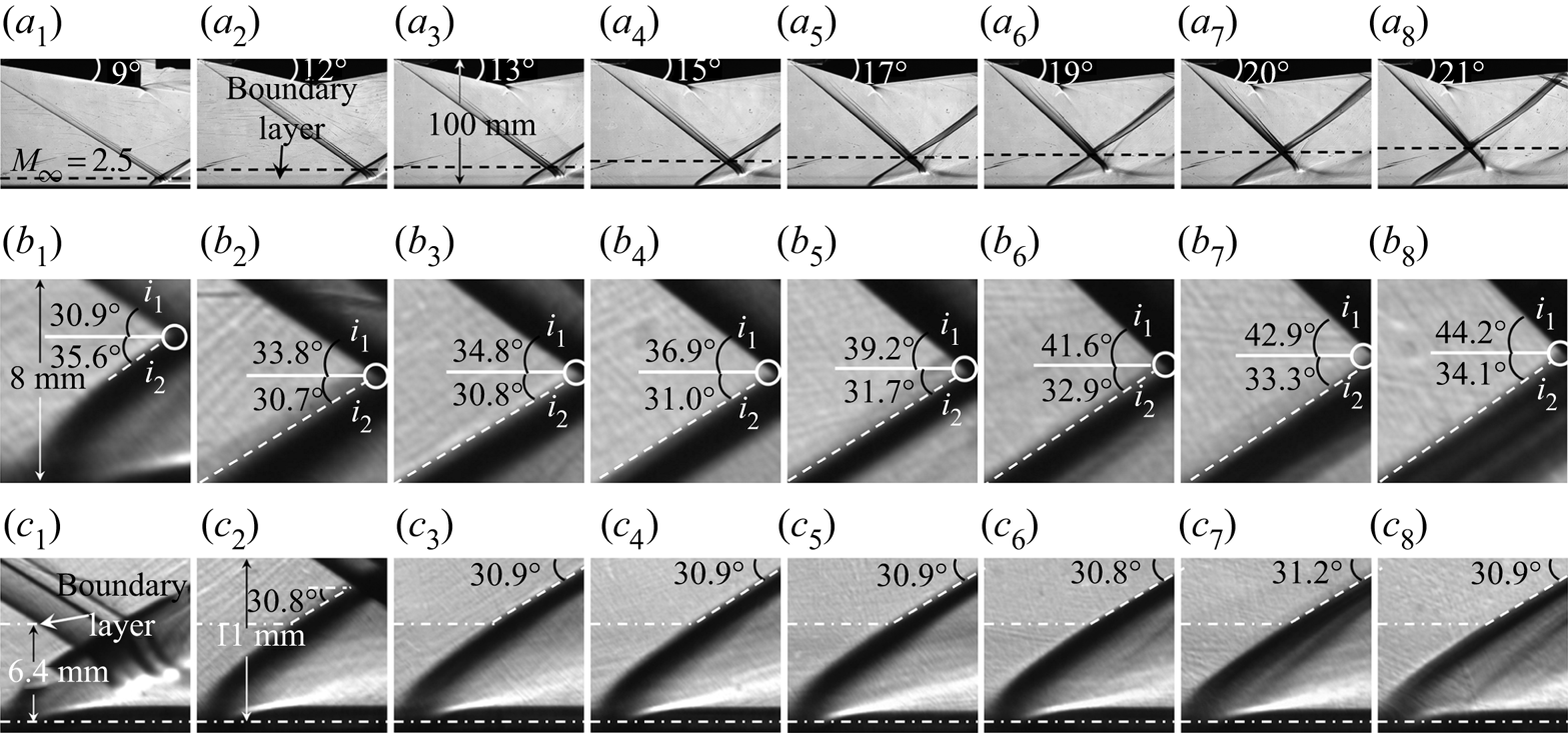
Figure 12 gives the schlieren images of overall flow fields and local flow fields induced by  $\alpha _1=9^\circ$,
 $12^\circ$,
 $13^\circ$,
 $15^\circ$,
 $17^\circ$,
 $19^\circ$,
 $20^\circ$ and
 $21^\circ$ shock generators, respectively, indicating a strong influence of incident shock strength on SWBLI. As is indicated in figure 12, there is no doubt that the separation shock is a curved shock due to the differentiation between separation shock angles measured on starting and ending portions, including angles close to the interaction point denoted as
 $\beta _{\textit {Exp}.\,\textit {int}.}$ shown in figure12(
 $b_1$–
 $b_8$) and angles close to the boundary layer denoted as
 $\beta _{\textit {Exp}.\,bou.}$ shown in figure 12(
 $c_1$–
 $c_8$). The interaction point of the
 $9^\circ$ wedge is inside of the boundary layer following a very curved separation shock bending downward, as shown in figure 12(
 $c_1$). The interaction points of other wedges, as shown in figure 12(
 $c_2$–
 $c_8$), are out of the boundary layer with similar separation shock angles of
 $\beta _{\textit {Exp.}\,\textit{bou}.}\approx 30.9^\circ$, which agrees well with the FIT solution of
 $\beta _{\textit {FIT}0}\approx 30.8^\circ$, meanwhile, in figure 12(
 $b_2$–
 $b_8$), the separation shock angles close to the interaction point are distinctly different with
 $\beta _{\textit {Exp}.\,\textit {int}.}$ increasing from
 $30.7^\circ$ to
 $34.1^\circ$, which is close to the MEP solution of
 $\beta _{\textit {MEP}}$ ranging from
 $29.1^\circ$ to
 $33.8^\circ$ changed by the incident shock strength. For the
 $9^\circ$ wedge with
 $\beta _{\textit {MEP}}\ll \beta _{\textit {FIT}0}$, the interaction point is inside of the boundary layer followed by a relatively small separation bubble, corresponding to figure 9(
 $c$); for the
 $12^\circ$ and
 $13^\circ$ wedges with
 $\beta _{\textit {MEP}}<\beta _{\textit {FIT}0}$, the separation shock angles, which are slightly decreased from a lower portion to a higher one, seem to be suppressed by interaction points, resulting in convex separation shocks corresponding to figure 9(
 $b$); for the
 $15^\circ$ wedge with
 $\beta _{\textit {MEP}}\approx \beta _{\textit {FIT}0}$, the separation shock is straight, which corresponds to figure 9(
 $a$); for the
 $17^\circ$ to
 $21^\circ$ wedges with
 $\beta _{\textit {MEP}}>\beta _{\textit {FIT}0}$, however, the separation shock angle is increased with a distinctly growing separation bubble, resulting in concave separation shocks, which correspond to figure 9(
 $d$).
Schlieren images of SWBLI at  $M_\infty =2.5$,
 $AR_{eff}=1.50$:
 $(a_1)\text {--}(a_8)$ are overall flow fields of
 $\alpha _1=9^\circ$ to
 $\alpha _1=21^\circ$, respectively,
 $(b_1)\text {--}(b_8)$ are local flow fields close to interaction point of
 $\alpha _1=9^\circ$ to
 $\alpha _1=21^\circ$, respectively, and
 $(c_1)\text {--}(c_8)$ are local flow fields close to boundary layer of
 $\alpha _1=9^\circ$ to
 $\alpha _1=21^\circ$, respectively.
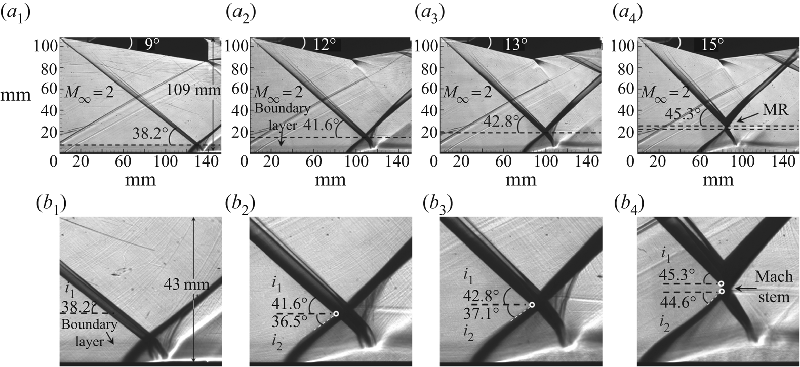
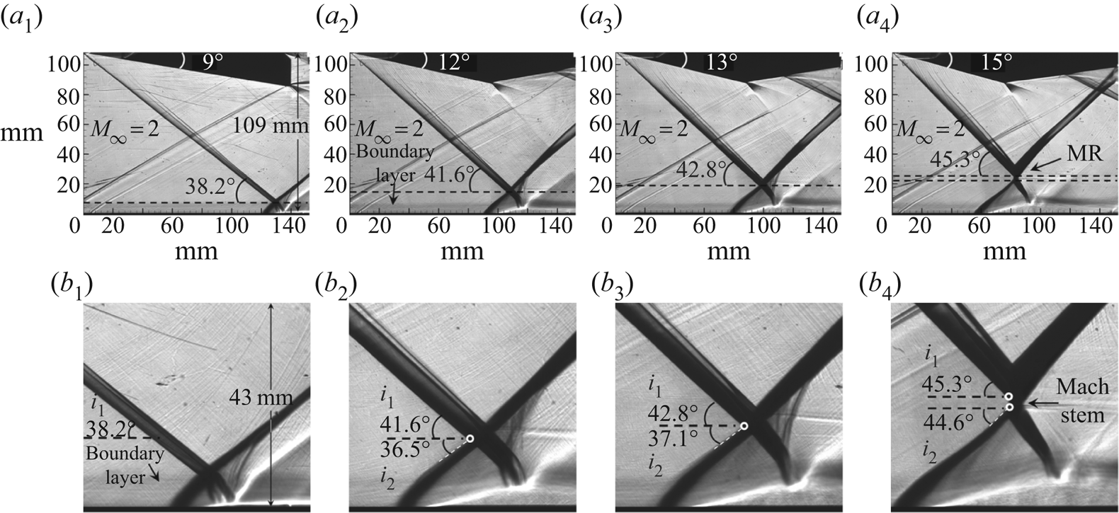
Similar patterns are observed from the tests conducted at  $M_\infty =2$,
 $AR_{eff}=1.38$, on four wedges including
 $\alpha _1=9^\circ$,
 $12\,^\circ$,
 $13\,^\circ$ and
 $15\,^\circ$, as shown in figure 13. The FIT solutions under the current conditions are
 $\beta _{\textit {FIT}0}\approx 37.5^\circ$, while ideal MEP solutions for RR are
 $\beta _{{\textit{MEP}}9^\circ }=34.5^\circ$,
 $\beta _{\textit{MEP}12^\circ }=36.2^\circ$ and
 $\beta _{\textit{MEP}13^\circ }=36.8^\circ$ (flow transited to MR with
 $\alpha _1\geq 15^\circ$), respectively. The interaction point of the
 $9^\circ$ wedge with
 $\beta _{\textit {MEP}}\ll \beta _{\textit {FIT}0}$ is still inside of the boundary layer, leading to a small separation, as shown in figures13(
 $a_1$) and 13(
 $b_1$). The other wedges (
 $\alpha _1=12^\circ$ to
 $15^\circ$) demonstrate a stable separation shock angle close to the boundary layer with
 $\beta _{\textit {Exp}.\,\textit{bou}.}\approx 37.3^\circ$, while angles close to the interaction point are
 $\beta _{\textit {Exp}.\,\textit {int}.}=36.5^\circ$,
 $37.1^\circ$ and
 $44.6^\circ$, respectively, followed by a separation bubble growing gradually, as shown in figure 13(
 $b_2$–
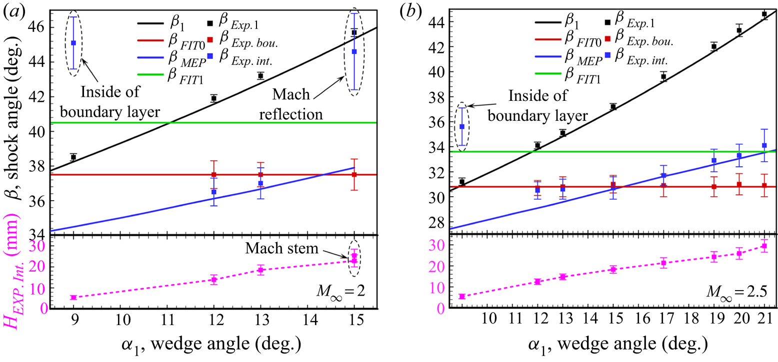
 $b_4$). In order to conduct a comprehensive analysis, the major angles of theoretical results and measured angles from schlieren images are summarized in figure 14, which gives the statistical results with time average and error bars obtained from more than 200 successive schlieren images for each case.
Schlieren images of SWBLI at  $M_\infty =2$,
 $AR_{eff}=1.38$:
 $(a_1)\text {--}(a_4)$ are overall flow fields of
 $\alpha _1=9^\circ$ to
 $\alpha _1=15^\circ$, respectively, and
 $(b_1)\text {--}(b_4)$ are local flow fields of
 $\alpha _1=9^\circ$ to
 $\alpha _1=15^\circ$, respectively.
Statistics of shock angles for contrast between theoretical solutions (ideal conditions without disturbance) and experimental results (total pressure 4 bar, total temperature 285 K): ( $a$)
 $M_\infty =2$,
 $AR_{eff}=1.38$ and (
 $b$)
 $M_\infty =2.5$,
 $AR_{eff}=1.50$.
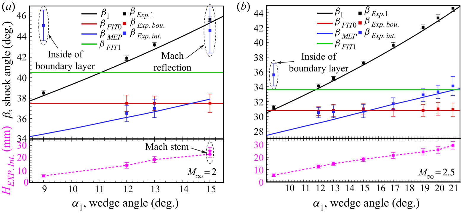
As is indicated in figure 14, the uncertainties of  $\beta _{\textit {Exp}.\,\textit {int}.}$ and interaction point height
 $H_{\textit {Exp}.\,\textit {int}.}$ are intensified with the increasing of incident shock strength, especially in MR configuration shown in figure 14(
 $a$), which means a larger separation bubble is more unstable than a smaller one. When the interaction point is out of the boundary layer, i.e. except
 $\alpha _1=9^\circ$,
 $\beta _{\textit {Exp}.\,\textit{bou}.}$ agrees well with the FIT solution
 $\beta _{\textit {FIT}0}$, meanwhile
 $\beta _{\textit {Exp}.\,\textit {int}.}$ grows approximately along the line of MEP solution
 $\beta _{\textit {MEP}}$ with the increasing of
 $\alpha _1$, and it agrees well with
 $\beta _{\textit {MEP}}$ when
 $\beta _{\textit {MEP}}\geq \beta _{\textit {FIT}0}$ at
 $M_\infty =2.5$, shown in figure 14(
 $b$). Additionally, with the growth of separation shock strength, a convex separation shock exists in
 $\beta _{\textit {MEP}}<\beta _{\textit {FIT}0}$, while a concave separation shock exists in
 $\beta _{\textit {MEP}}>\beta _{\textit {FIT}0}$, and when separation shock strength grows strong enough, the flow configuration would be transited to MR, which proves the flow patterns shown in figure 9(
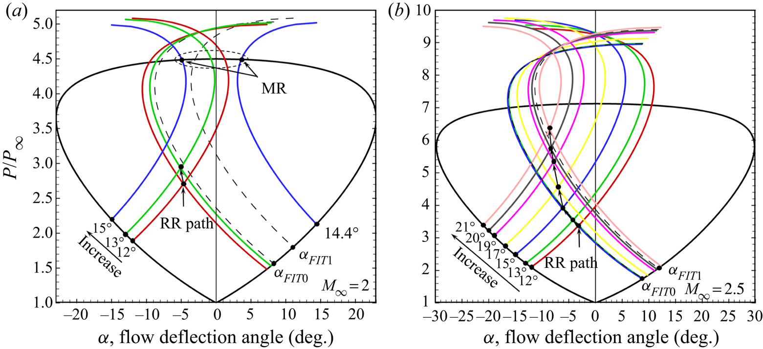
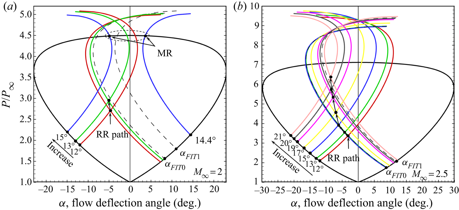
 $e$). The interaction solution of SWBLI is shown in figure 15 by shock polar lines. In figure15(
 $b$), separation shock is very close to
 $\beta _{\textit {FIT}0}$ with
 $\alpha _1\leq 15^\circ$ because the interaction point is close to the boundary layer, however, separation shock strength grows distinctly with
 $\alpha _1>15^\circ$ due to the interaction point getting further away from the boundary layer. Both figures 14 and 15 demonstrate that separation shock strength is not a constant value but could be changed by incident shock strength, and the effect of MEP solution on SWBLI is characterized by suppressing the growth of separation shock strength as well as separation bubble size with
 $\beta _{\textit {MEP}}<\beta _{\textit {FIT}0}$ while intensifying the growth with
 $\beta _{\textit {MEP}}>\beta _{\textit {FIT}0}$. Additionally, although flow deflection angles of
 $19^\circ$,
 $20^\circ$ and
 $21^\circ$ have reached the detachment condition angle of
 $17.95^\circ$ for
 $M_\infty =2.5$, while the solutions shown in figure15(
 $b$) are still residing in RR domain, indicating the RR to MR transition might be delayed by the interaction of incident shock and separation shock according to the MEP solution.
Interaction solution path of SWBLI on shock polar lines changed by incident shock strength: ( $a$)
 $M_\infty =2$,
 $AR_{eff}=1.38$ and (
 $b$)
 $M_\infty =2.5$,
 $AR_{eff}=1.50$.
4.2. Influence of the FIT solution on SWBLI
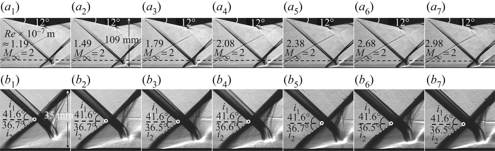
In order to research the effect of the FIT solution on SWBLI, the following tests are conducted on the  $12^\circ$ wedge at
 $M_\infty =2$,
 $AR_{eff}=1.38$,
 $T_0=285\ \textrm {K}$ with various unit Reynolds numbers of free stream:
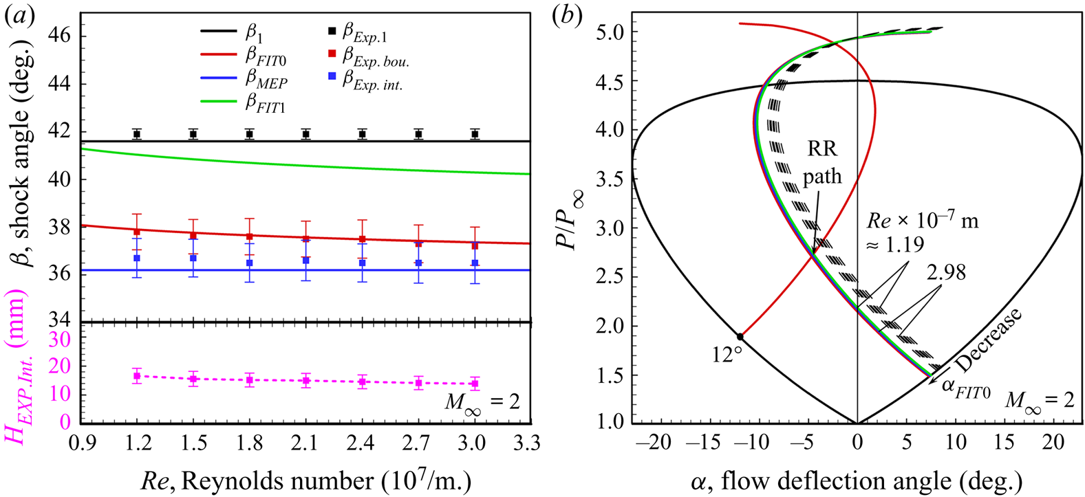
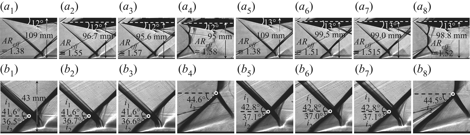
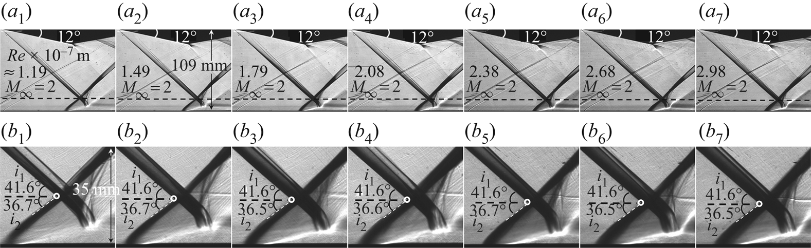
 $\mathit {Re}\times 10^{-7}\ \textrm {m}\approx 1.19$, 1.49, 1.79, 2.08, 2.38, 2.68 and 2.98. Figure 16 gives the evolution of SWBLI with schlieren images, indicating the flow configuration is not so sensitive to the change of Reynolds number. The separation shock is still a convex shock, because the MEP solution for the
 $12^\circ$ wedge is
 $\beta _{\textit{MEP}12^\circ }=36.2^\circ$, while the FIT solution
 $\beta _{\textit {FIT}0}$ decreases slightly from
 $37.9^\circ$ to
 $37.3^\circ$ with Reynolds number increasing from
 $1.19\times 10^7/\textrm {m}$ to
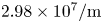 $2.98\times 10^7/\textrm {m}$.
Schlieren images of SWBLI at  $M_\infty =2$,
 $AR_{eff}=1.38$:
 $(a_1)\text {--}(a_7)$ are overall flow fields of
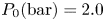 $P_0 (\textrm {bar})=2.0$ to 5.0, respectively, and
 $(b_1)\text {--}(b_7)$ are local flow fields of
 $\mathit {Re}\times 10^{-7}\ \textrm {m}\approx 1.19$, 1.49, 1.79, 2.08, 2.38, 2.68 and 2.98, respectively.
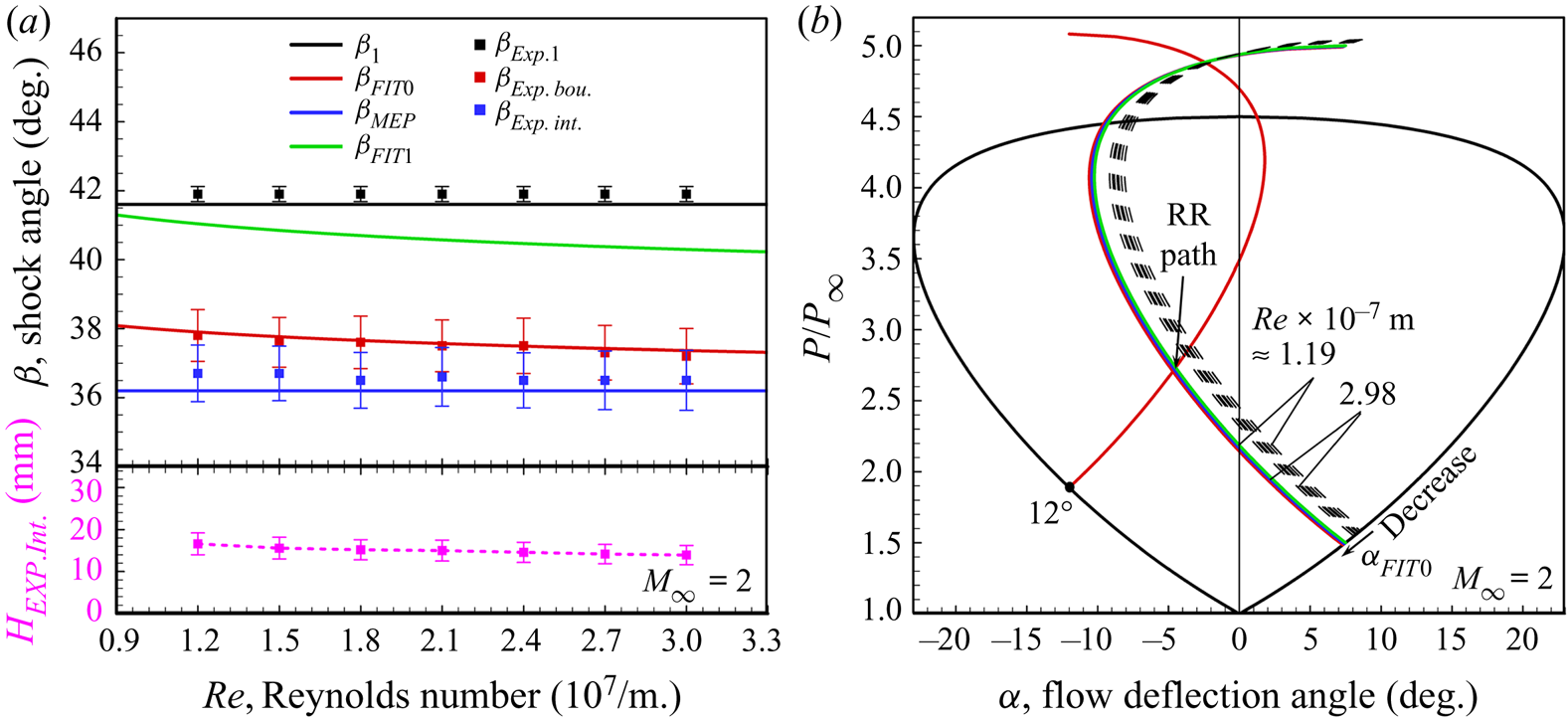
The major angles as well as the RR solution path on shock polar lines are summarized in figure 17. It could be observed from figure 17( $a$) that
 $\beta _{\textit {Exp}.\,\textit {bou}.}$ decreases slightly, which agrees well with
 $\beta _{\textit {FIT}0}$, meanwhile the change of
 $\beta _{\textit {Exp}.\,\textit {int}.}$, which is a little larger than
 $\beta _{{MEP}12^\circ }$, is not so distinct. It should be noticed that the interaction point height
 $H_{\textit {Exp}.\,\textit {int}.}$ decreases almost linearly with the increasing of Reynolds number and decreasing of boundary layer thickness, meaning lower
 $\beta _{\textit {FIT}0}$ corresponds to smaller separation bubble size. In figure 17(
 $b$), although the polar line of
 $\beta _{\textit {FIT}0}$ moves downward in a small range, the RR solution path is almost stable. Therefore, the influence of Reynolds number in the range from
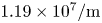 $1.19\times 10^7/\textrm {m}$ to
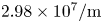 $2.98\times 10^7/\textrm {m}$ on SWBLI is very weak compared with the influence of incident shock strength mentioned above.
Statistics of shock angles and interaction solution path at  $M_\infty =2$,
 $\alpha _1=12^\circ$,
 $AR_{eff}=1.38$: (
 $a$) contrast between theoretical solutions and experimental results, (
 $b$) RR solution path of SWBLI on shock polar lines changed by Reynolds number.
4.3. Influence of installation height of model on SWBLI
The downstream expansion fan might affect SWBLI with models mounted at a high position, which has been proved by the work of Grossman & Bruce (Reference Grossman and Bruce2018) on models mounted at  $AR_{eff}=1$ with various thicknesses. Therefore, the effect of models mounted at a low position on SWBLI should be taken into consideration, and further tests are conducted on the
 $12^\circ$ and
 $13^\circ$ wedges in
 $M_\infty =2$,
 $P_0=4.0\ \textrm {bar}$,
 $T_0=285\ \textrm {K}$ flow with the installation height reduced gradually from
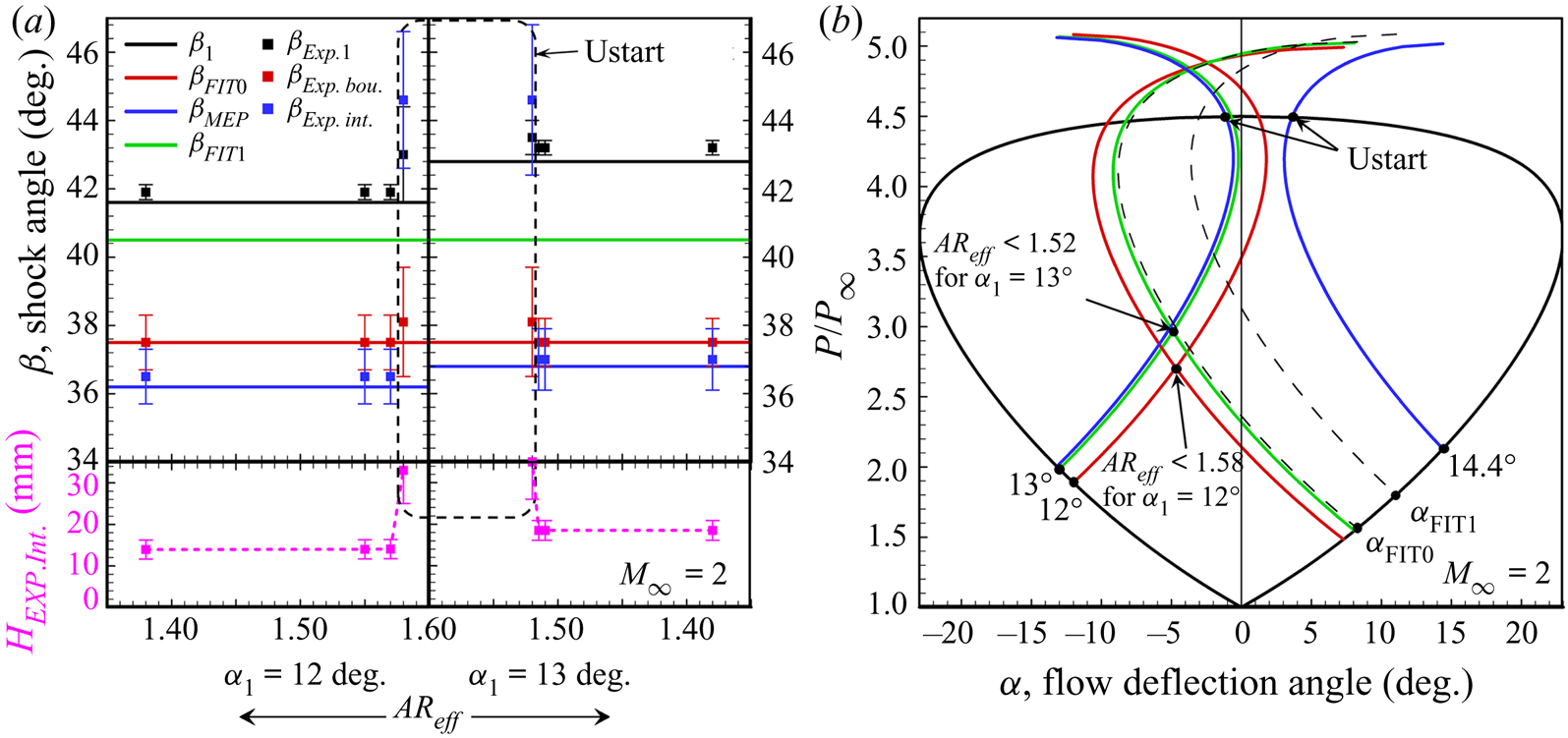
 $AR_{eff}=1.38$ till unstart, as shown in figure18. The flow fields induced by the
 $12^\circ$ wedge are shown in figure 18(
 $a_1$–
 $a_4$) with
 $AR_{eff}$ increasing from 1.38 to 1.58, where the SWBLI configuration is observed relatively stable in starting flows of
 $AR_{eff}<1.58$. Similar patterns are observed on the
 $13^\circ$ wedge shown in figure 18(
 $a_5$–
 $a_8$), while starting flows exist in
 $AR_{eff}<1.52$, which is lower than that in the
 $12^\circ$ wedge flow.
Schlieren images of SWBLI at  $M_\infty =2$:
 $(a_1)\text {--}(a_4)$ are overall flow fields of
 $\alpha _1=12^\circ$ with
 $AR_{eff}=1.38$, 1.55, 1.57 and 1.58, respectively,
 $(a_5)\text {--}(a_8)$ are overall flow fields of
 $\alpha _1=13^\circ$ with
 $AR_{eff}=1.38$, 1.55, 1.57 and 1.58, respectively and
 $(b_1)\text {--}(b_8)$ are local flow fields corresponding to
 $(a_1)\text {--}(a_8)$, respectively.
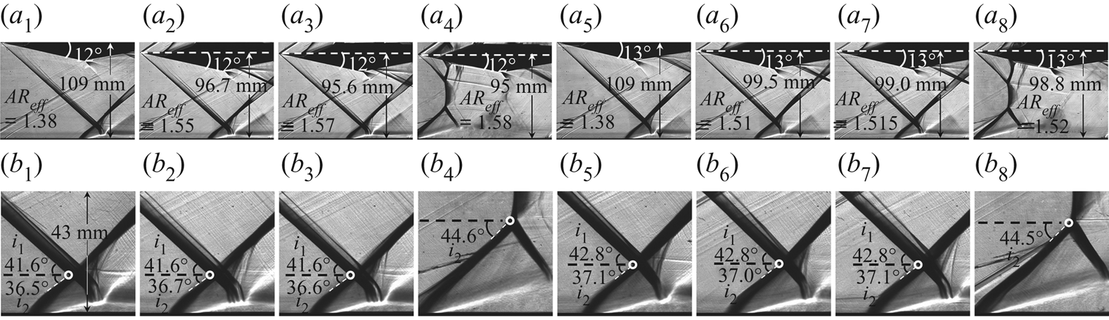
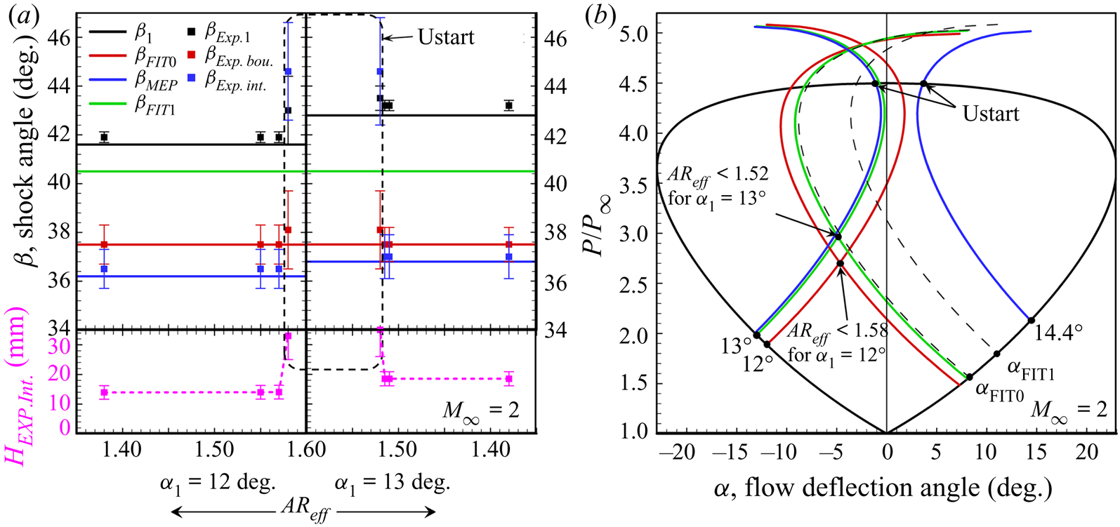
Figure 19 gives the major angles and solution path on shock polar lines, in which separation shock angles agree well with theoretical results in starting flow and the effect of  $AR_{eff}$ on the RR solution path is not distinct, indicating the influence of reducing model height from
 $AR_{eff}=1.38$ till unstart on SWBLI is very weak before the appearance of unstart. Therefore, the RR configuration of SWBLI mostly depends on incident shock strength compared with model mounted position.
Statistics of shock angles and interaction solution path at  $M_\infty =2$,
 $\alpha _1=12^\circ$ and
 $13^\circ$: (
 $a$) contrast between theoretical solutions and experimental results and (
 $b$) solution path of SWBLI on shock polar lines changed by installation height of model.
5. Conclusions
The current study couples the FIT method with the MEP method to determine the appearance of separation shock, which agrees well with current experiments performed at Mach number 2 and 2.5. The proposed model could predict separation shock angle in regular SWBLI, while it does not apply well to very small separation inside of the boundary layer or very large separation of Mach reflection, based on which the following conclusions are obtained.
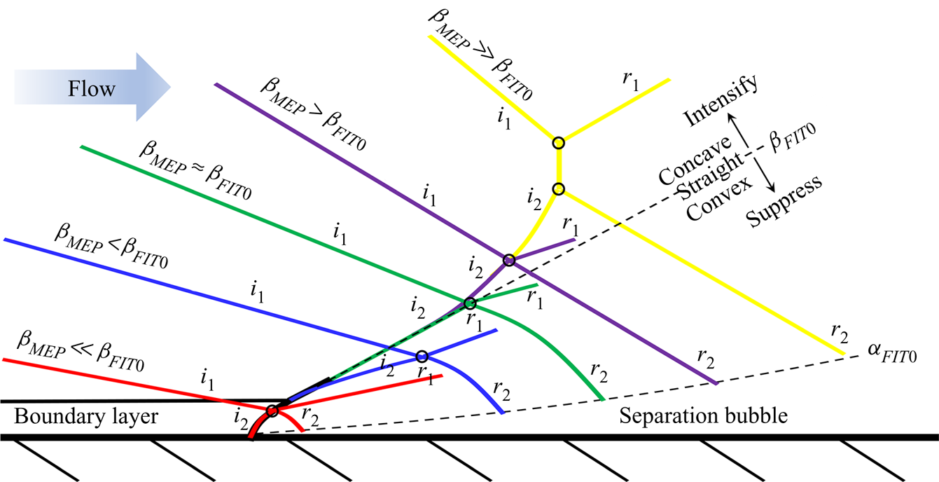
The FIT solution contributes to the initial separation shock angle close to the boundary layer, while the MEP solution could be in charge of the final separation shock strength close to the shock–shock interaction point, which is described by figure 20. On one hand, separation shock strength as well as separation bubble size might be suppressed with  $\beta _{\textit {MEP}}<\beta _{\textit {FIT}0}$, resulting in a convex separation shock and a small separation bubble, and the interaction point could be inside of the boundary layer with
 $\beta _{\textit {MEP}}\ll \beta _{\textit {FIT}0}$; on the other hand, separation is intensified with
 $\beta _{\textit {MEP}}>\beta _{\textit {FIT}0}$, leading to a concave separation shock and a large separation bubble, and RR to MR transition might exist in
 $\beta _{\textit {MEP}}\gg \beta _{\textit {FIT}0}$ with separation shock strength reaching to the detachment criterion.
Sketch for illustrating various configurations of SWBLI according to the relation between FIT and MEP solutions.
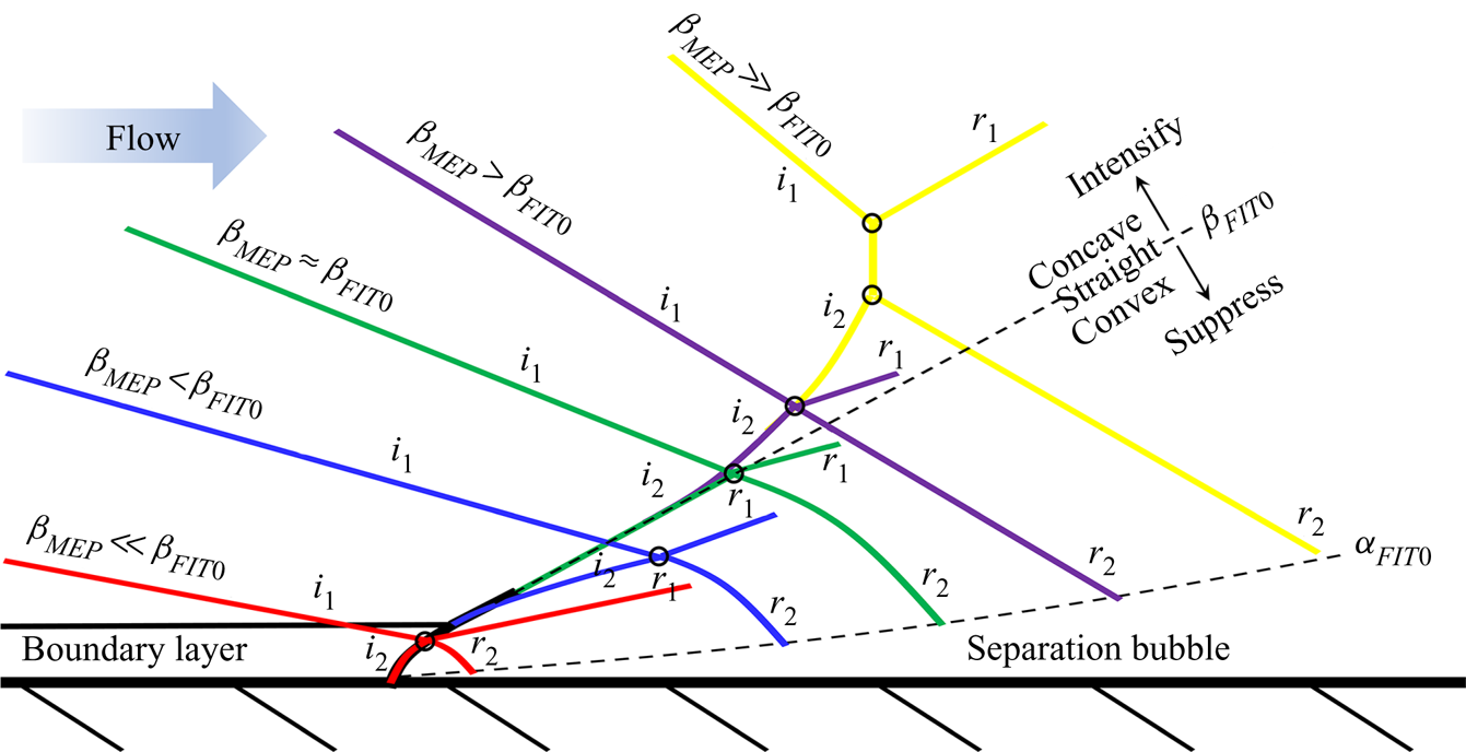
The configuration of SWBLI depends on incoming flow properties and incident shock strength, and smaller separation is more likely to exist in the situations of lower skin friction coefficient, higher incoming Mach numbers and weaker incident shock waves. The SWBLI is much more sensitive to incident shock strength than incoming flow properties, by contrast, the effects of Reynolds number and model mounting height might be relatively weak.
Acknowledgments
This work was supported by the National Natural Science Foundation of China (51776096) and China Postdoctoral Science Foundation (YBA19067). This support is gratefully acknowledged. We thank PhD candidate S. Liu for the assistance in all the experiments.
Declaration of interests
The authors report no conflict of interest.