







1. Introduction
Convective cumulus clouds in the atmosphere tend to have a structure resembling cauliflower. This impression naturally leads to an interpretation that these convective clouds consist of many quasi-spherical thermal bubbles, as proposed by Scorer & Ludlam (Reference Scorer and Ludlam1953). For this reason, extensive studies of thermal bubbles were performed over the period of the 1950s to 1960s with the goal of understanding atmospheric convection better, as reviewed by Ludlam & Scorer (Reference Ludlam and Scorer1953) and Yano (Reference Yano2014). An idealized thermal can be experimentally generated by releasing an isolated buoyancy anomaly from a surface. Because it develops into a vortex ring, such a thermal may be more precisely called a thermal vortex ring; the present study adopts this terminology. Recently, there are substantial numbers of numerical studies on these idealized isolated thermals both for the dry (Tarshish, Jeevanjee & Lecoanet Reference Tarshish, Jeevanjee and Lecoanet2018; Lecoanet & Jeevanjee Reference Lecoanet and Jeevanjee2019; McKim, Jeevanjee & Lecoanet Reference McKim, Jeevanjee and Lecoanet2020; Morrison, Jeevanjee & Yano Reference Morrison, Jeevanjee and Yano2022; Morrison et al. Reference Morrison, Jeevanjee, Lecoanet and Peters2023) and moist cases (Morrison Reference Morrison2016a,Reference Morrisonb; Morrison & Peters Reference Morrison and Peters2018; Morrison, Peters & Sherwood Reference Morrison, Peters and Sherwood2021; Vybhav & Ravichandran Reference Vybhav and Ravichandran2022) thanks to increased computational power. Here, moist cases behave qualitatively differently from dry counterparts due to the latent heating and cooling associated with condensation and evaporation of cloud condensate.
From a theoretical perspective, studies of thermal vortex rings can be considered a natural extension of ‘inertial’ vortex rings, that is, vortex rings without buoyancy forcing. Various theoretical solutions of steadily propagating ‘inertial’ vortex rings were identified by Hill (Reference Hill1894), Hick (1884), Fraenkel (Reference Fraenkel1972), Norbury (Reference Norbury1972, Reference Norbury1973) and Sullivan et al. (Reference Sullivan, Niemela, Hershberger, Bolster and Donnelly2008). However, these existing theoretical solutions can only describe steadily propagating states. Recently, Yano & Flierl (Reference Yano and Flierl2024) attempted to generalize the Hill's vortex solution by including buoyancy in the system, and to describe analytically the regime traditionally presented by a similarity solution (Scorer Reference Scorer1957). However, the similarity solution is not applicable to the initial spin-up stage.
Even today, the main theoretical bases for interpreting the dynamics of thermal vortex rings remain classical studies by Scorer (Reference Scorer1957) and Turner (Reference Turner1957) in terms of dimensional analysis and impulse dynamics. Yano (Reference Yano2023) recently revisited these studies from the point of view of the vortex dynamics, and derived Scorer's similarity solution in a self-consistent manner from this perspective. Yano (Reference Yano2023) also derived theoretical constraints to be satisfied over the similarity regime, which can be used to test the consistency of numerical simulations.
Yano (Reference Yano2023) further suggested a general formulation for describing the evolution of a thermal vortex ring in terms of volume integrals of various vorticity moments (e.g. circulation, impulse), which is applicable to both the similarity regime as well as an initial vortex-ring spin-up stage. Due to unspecified geometrical factors involved in this formulation, however, it does not provide a closed description. Nevertheless, it provides a consistent framework to interpret the evolution of a thermal vortex ring from the point of view of the vortex dynamics. The proposed analysis formulation therein provides an alternative framework to momentum budget analysis for describing the dynamics of convective cloud elements, as pursued by, e.g. Morrison (Reference Morrison2016a, Reference Morrison2017), and Morrison & Peters (Reference Morrison and Peters2018), and complements the latter.
The purpose of the present study is to apply the formulation proposed by Yano (Reference Yano2023) based on the vortex dynamics for interpreting a high-resolution simulation of a thermal vortex ring recently described by Morrison et al. (Reference Morrison, Jeevanjee and Yano2022). It was shown by Turner (Reference Turner1957) that the impulse dynamics can lead to a similarity solution of a thermal vortex ring, as suggested by Scorer (Reference Scorer1957) following a dimensional analysis. The present study extends this description to the initial spin up by adding the volume integrals of vorticity and potential vorticity as prognostic variables of the system. In this manner, the present study adopts the theoretical framework for describing the thermal vortex ring developed by Yano (Reference Yano2023), and applies this framework to analyse a thermal vortex-ring numerical simulation.
After briefly reviewing the numerical simulation described by Morrison et al. (Reference Morrison, Jeevanjee and Yano2022) in the next section, the vortex dynamics is introduced in § 3, and the simulation is analysed under a framework of the volume-integrated bulk vorticity budgets in § 4 by following Yano (Reference Yano2023). The main conclusion from the analysis is that the non-axisymmetric component of the flow, though non-negligible, has only a limited impact on the bulk vorticity budgets. This further suggests that the simulated thermal vortex-ring dynamics can be interpreted as a type of two-dimensional, axisymmetric flow. This possibility is explored further in § 5. The paper is closed by a summary and additional discussion in § 6.
2. Simulation
We analyse the high-resolution simulation case (HIGHRES) in Morrison et al. (Reference Morrison, Jeevanjee and Yano2022, hereafter MJY). This simulation uses  $560\times 560$ grid points in the horizontal and
 $800$ in the vertical with a grid spacing of
 $\Delta x =0.02$ in non-dimensional units. The initial condition consists of a spatially uniform spherical buoyancy anomaly with a unit non-dimensional radius and a unit non-dimensional value for the buoyancy, with weak random perturbations (
 ${\pm }0.1$) to the buoyancy superposed. In MJY, four additional runs were performed with different initial perturbations (using different random number seeds) to ensure that the overall evolution does not sensitively depend on the particular initial perturbations applied. The intention of this simulation is, within the limit of available resolution, to reproduce the evolution of a thermal vortex ring in high-Reynolds-number flow as accurately as possible. Thus, here a large-eddy simulation (cf. Sagaut Reference Sagaut2002) is performed with a subgrid-scale (SGS) mixing scheme by Stevens, Moeng & Sullivan (Reference Stevens, Moeng and Sullivan1999), which effectively works as a weak dissipation term.
A basic principle of large-eddy simulation is to model a flow under the asymptotic limit of a large Reynolds number ( $Re \to \infty$), yet the unresolved small eddies are implicitly represented by the SGS scheme (with additional dissipation from numerical diffusion). Thus, results are sensitive to the adopted model resolution as shown in MJY. Also, keep in mind that no background stratification is introduced in this simulation, implying a Froude number (based on the background stratification) of
 $Fr \to \infty$. The Froude number can be alternatively defined as a non-dimensional measure of the inverse of the vortex-ring buoyancy anomaly (ratio of thermal inertia divided by buoyant forcing), as originally introduced by Scorer (Reference Scorer1957). This is defined by (6) in MJY and plotted in their figure 8(c) for the present simulation. According to this plot, the Froude number is about 1.1–1.3 consistent with previous thermal studies (e.g. Scorer Reference Scorer1957; Turner Reference Turner1964).
A thermal tracking algorithm to determine thermal boundaries and propagation speed is similar to that used by Lecoanet & Jeevanjee (Reference Lecoanet and Jeevanjee2019). We refer readers interested in details of the simulations and thermal tracking algorithm to the original paper (MJY). In the following, as in MJY, all results are presented in non-dimensional units.
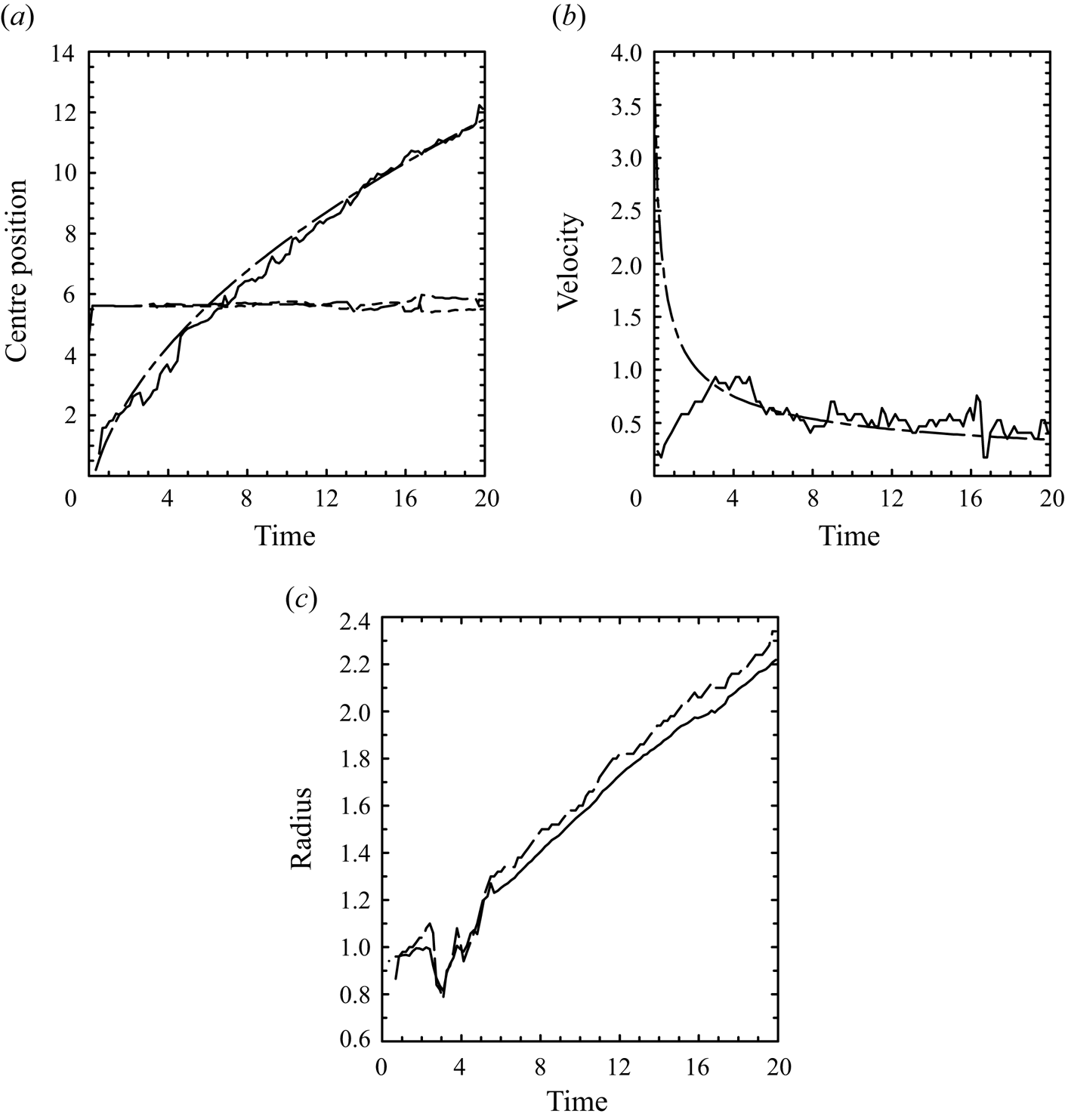
Basic characteristics of the simulated thermal vortex ring are calculated by MJY and shown in figure 1 for the full period of the simulation. Here, especially, the equivalent radius is defined as a radius of a spherical thermal with the same volume as the simulation. Note that the simulated thermal vortex ring is not perfectly spherical, as seen by a discrepancy between the equivalent radius (solid) and the equatorial radius (long dash) in figure 1(c). The evolutions of the vortex-ring height,  $z$, and the propagation velocity,
 $\bar {w}$, are seen to follow the similarity solutions closely after an initial spin-up period (
 $t=0\unicode{x2013}3$). Here, the end of the spin-up period (
 $t \simeq 3$) may be identified as the crossing point of the numerically obtained
 $\bar {w}$ with the similarity curve in figure 1(b). The fits to the similarity solutions are made by following the methodology detailed in MJY.
Basic characteristics of the simulated thermal vortex ring as a function of time: (a) centre position of the vortex ring:  $x$ (long dash),
 $y$ (short dash) and
 $z$ (solid); (b) propagation velocity; (c) vortex-ring size: equivalent radius (solid) and equatorial radius (long dash). Fits to the tendencies expected from the similarity solutions are also added in (a,b) as chain-dashed curves.
3. Vortex dynamics
We adopt cylindrical coordinates,  $(s, \varphi, z)$, in the present study, in which
 $s$ is a radial distance of the vertical axis of the vortex ring,
 $\varphi$ the azimuthal angle and
 $z$ the vertical coordinate. Following Yano (Reference Yano2023), we focus on the budget of the azimuthal component,
 $\zeta$, of the vorticity, because it plays a primary role in the vortex-ring dynamics. After azimuthal averaging, its governing equation is given by
 \begin{equation} s\left(\frac{\partial}{\partial t}+\bar{u}_s\frac{\partial}{\partial s}+\bar{u}_z\frac{\partial}{\partial z}\right)\frac{\bar{\zeta}}{s} ={-} \frac{\partial \bar{b}}{\partial s} + \bar{G}.\end{equation}
Here, the overbar indicates an azimuthal average,
 \begin{equation} \overline{{(*)}} \equiv \frac{1}{2{\rm \pi}}\int^{2{\rm \pi}}_0 (*) \,{\rm d}\varphi,\end{equation}
 $b$ is the buoyancy and the velocity is denoted by
 $u$ with the corresponding components designated by subscripts. Note that only the axisymmetric component of the buoyancy,
 $\bar {b}$, appears in (3.1a), yet the eddy component,
 $b^{\prime }$, will be considered explicitly later in (4.18). The forcing,
 $\bar {G}$, due to the non-axisymmetric components on the right-hand side is defined by
 \begin{equation} \bar{G} ={-}\frac{\partial}{\partial s}\overline{u_s^{\prime}\zeta^{\prime}} +\frac{1}{s}\frac{\partial}{\partial s}s\overline{u_{\varphi}^{\prime}\zeta_s^{\prime}} +\frac{\partial}{\partial z}\left(-\overline{u_z^{\prime}\zeta^{\prime}} +\overline{u_{\varphi}^{\prime}\zeta_z^{\prime}} + \frac{\overline{u_{\varphi}^{\prime 2}}}{2s}\right) . \end{equation}
Notations for the variables are fairly standard:  $\zeta$,
 $\zeta _s$ and
 $\zeta _z$ are the vorticity components in
 $\varphi$,
 $s$ and
 $z$ directions, defined by
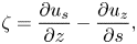 \begin{gather} \zeta = \frac{\partial u_s }{ \partial z} - \frac{\partial u_z }{ \partial s} , \end{gather}
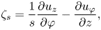 \begin{gather}\zeta_s = \frac{1}{s}\frac{\partial u_z }{ \partial \varphi} - \frac{\partial u_{\varphi} }{ \partial z} , \end{gather}
 \begin{gather}\zeta_z =\frac{1}{s}\frac{\partial}{ \partial s} s u_{\varphi} - \frac{1}{s}\frac{\partial u_s }{ \partial \varphi} . \end{gather}
Note that the diffusion terms are neglected from the analysis and assumed to be small, although the numerical simulation contains SGS mixing terms.
3.1. Coordinate transformation
To diagnose the terms in (3.1a,c) from the MYJ simulation, the output data natively on Cartesian coordinates,  $(x, y, z)$, are linearly interpolated to the cylindrical coordinate grid,
 $(s, \varphi, z)$ at each vertical height,
 $z$. The radial grid,
 $s_i$ (
 $i=1,\ldots, n$), is defined by taking the same grid spacing,
 $\Delta s(=\Delta x)$, as that of the original Cartesian coordinates with a total grid number of
 $n = 249$, with
 $i = 1$ corresponding to the origin,
 $s = 0$. The origin is defined as the centre point of the thermal following the thermal tracking algorithm of MYJ. This number,
 $n$, is chosen for convenience of the fast Fourier transformation later. The azimuthal coordinate,
 $\varphi$, is discretized by dividing the full circle into
 $8n$ points so as to take full advantage of the original resolution. In the following analysis, the differentials are evaluated by centred finite differences with the interpolated mesh sizes.
3.2. Diagnosis of the vorticity
The azimuthally averaged azimuthal component of vorticity,  $\bar {\zeta }$, whose budget is our major concern here, is diagnosed by two methods. First, the vorticity,
 $\zeta$, is diagnosed from the three-dimensional velocity field,
 $(u_s, u_{\varphi }, u_z)$, based on the definition (3.2a), then its azimuthal average is performed to obtain
 $\bar {\zeta }$. Second, the azimuthally averaged
 $\bar {\zeta }$ is directly diagnosed from the azimuthally averaged velocity field,
 $(\bar {u}_s, \bar {u}_z)$. Both evaluation methods lead to mutually consistent results in terms of the volume-integrated moments of the vorticity, which are the primary quantities examined in the following analysis. Results presented in the following are based on the second method.
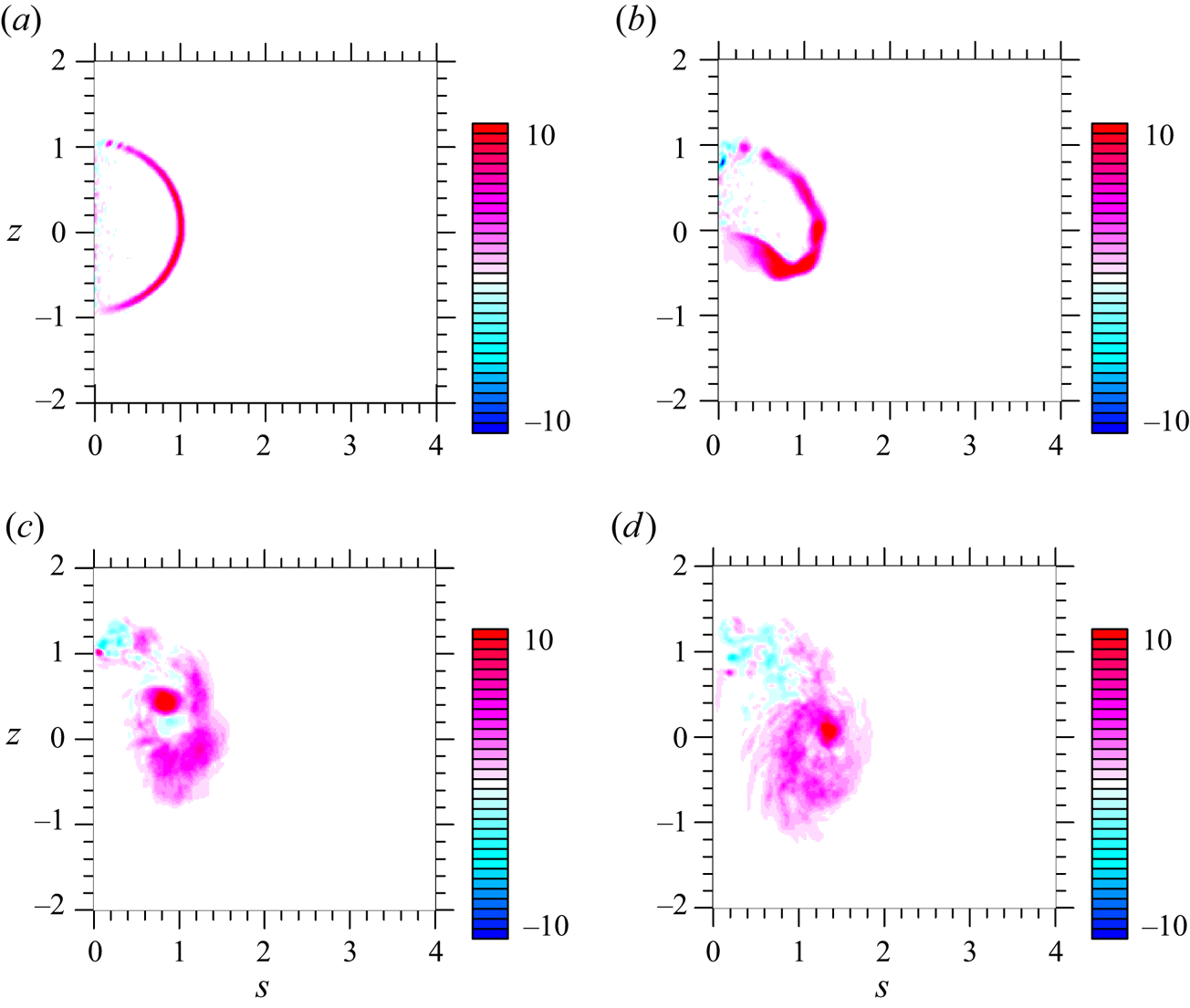
Evolution of  $\bar {\zeta }$ over the initial spin-up period is shown in figure 2. A vorticity sheet is rapidly generated along the initial buoyancy anomaly edge owing to the differential buoyancy force on the right-hand side of (3.1a) (a); this vortex sheet deforms and wraps into itself with time: from
 $t=2.5$ (b) to
 $t=4$ (c), leading to a vortex-ring core by
 ${t=5}$ (d).
Initial evolution of the azimuthally averaged azimuthal component of the vorticity,  $\bar {\zeta }$, over the period of
 $t=1\unicode{x2013}5.5$. Results are presented in coordinates moving upward following the vortex ring with the ring centre set to
 $z=0$. (a)
 $t = 1$, (b)
 $t = 2.5$, (c)
 $t = 4$ and (d)
 $t = 5.5$.
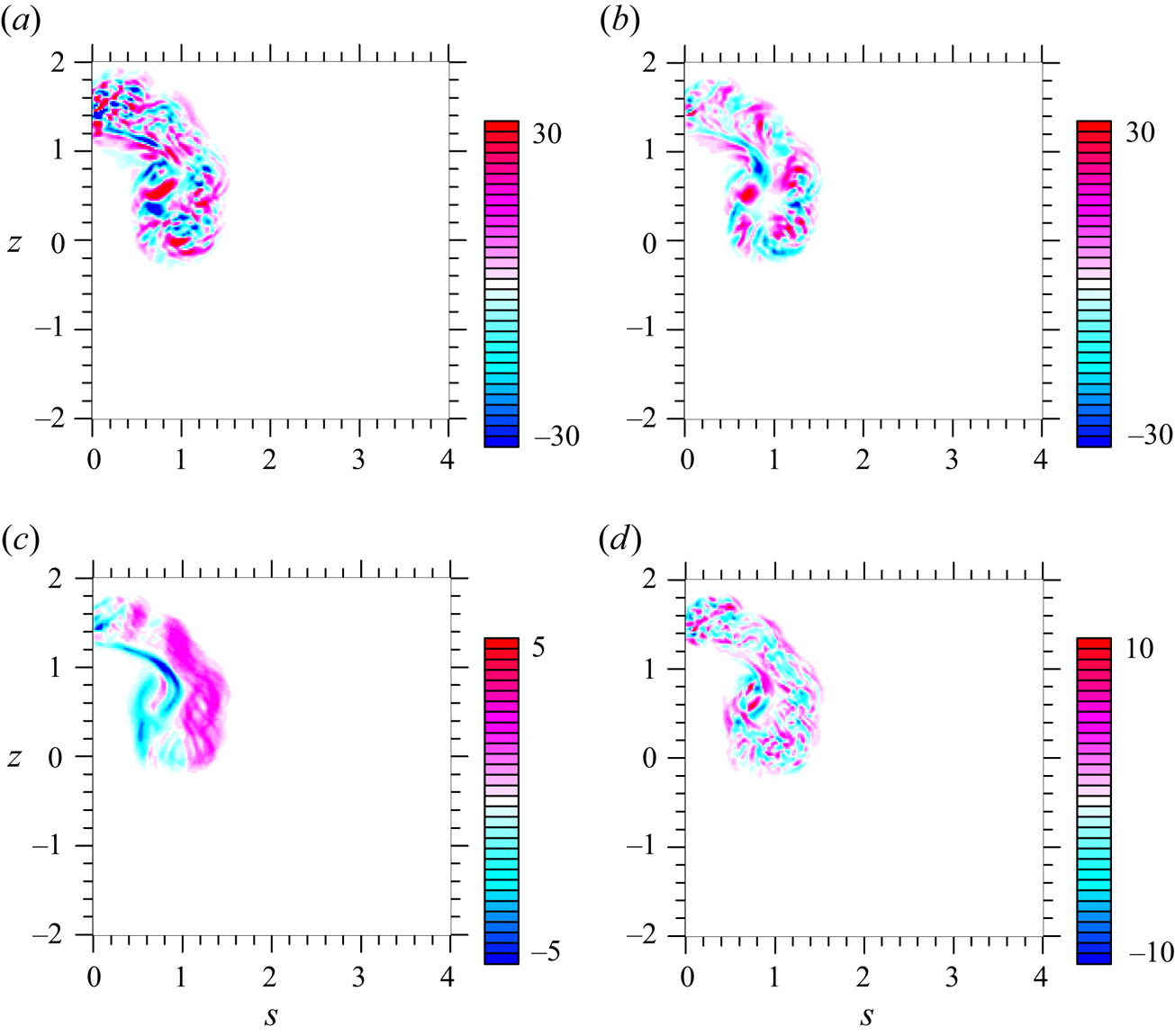
A snapshot of the vorticity-budget analysis based on (3.1a) at  $t = 3.4$ is shown in figure 3. The system begins to evolve axisymmetrically initially, and the non-axisymmetric forcing,
 $\bar G$ in figure 3(d), only develops gradually. As already remarked by commenting on figure 1(b), a steady vortex-ring form becomes established at roughly
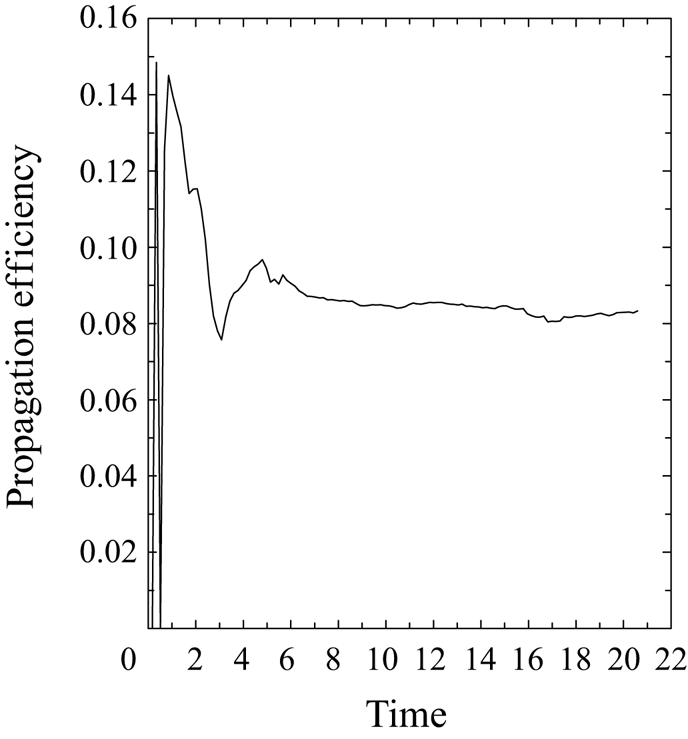
 $t \simeq 3$, after which the system is considered to be in the similarity regime. This time when spin up is achieved is also later in section 4.2 identified as a crossing point of the simulated value of
 $\tilde {v}_z$ with the final equilibrium value,
 $\tilde {v}_z \simeq 0.085$, in figure 5 later. Nevertheless, the spin-up time is only approximate since it cannot be defined precisely, as suggested by figure 4 below.
The vorticity budget, as defined by (3.1a) at  $t = 3.4$: (a) local tendency,
 $\partial \bar {\zeta }/\partial t$; (b) advection,
 $s{\bar {\boldsymbol {v}}}\boldsymbol {\cdot } \boldsymbol {\nabla }(\bar {\zeta }/s)$; (c) buoyancy forcing,
 $-\partial \bar {b}/\partial s$; and (d) non-axisymmetric forcing,
 $\bar {G}$. The analysis is performed on the system moving with the vortex ring by its propagation speed.
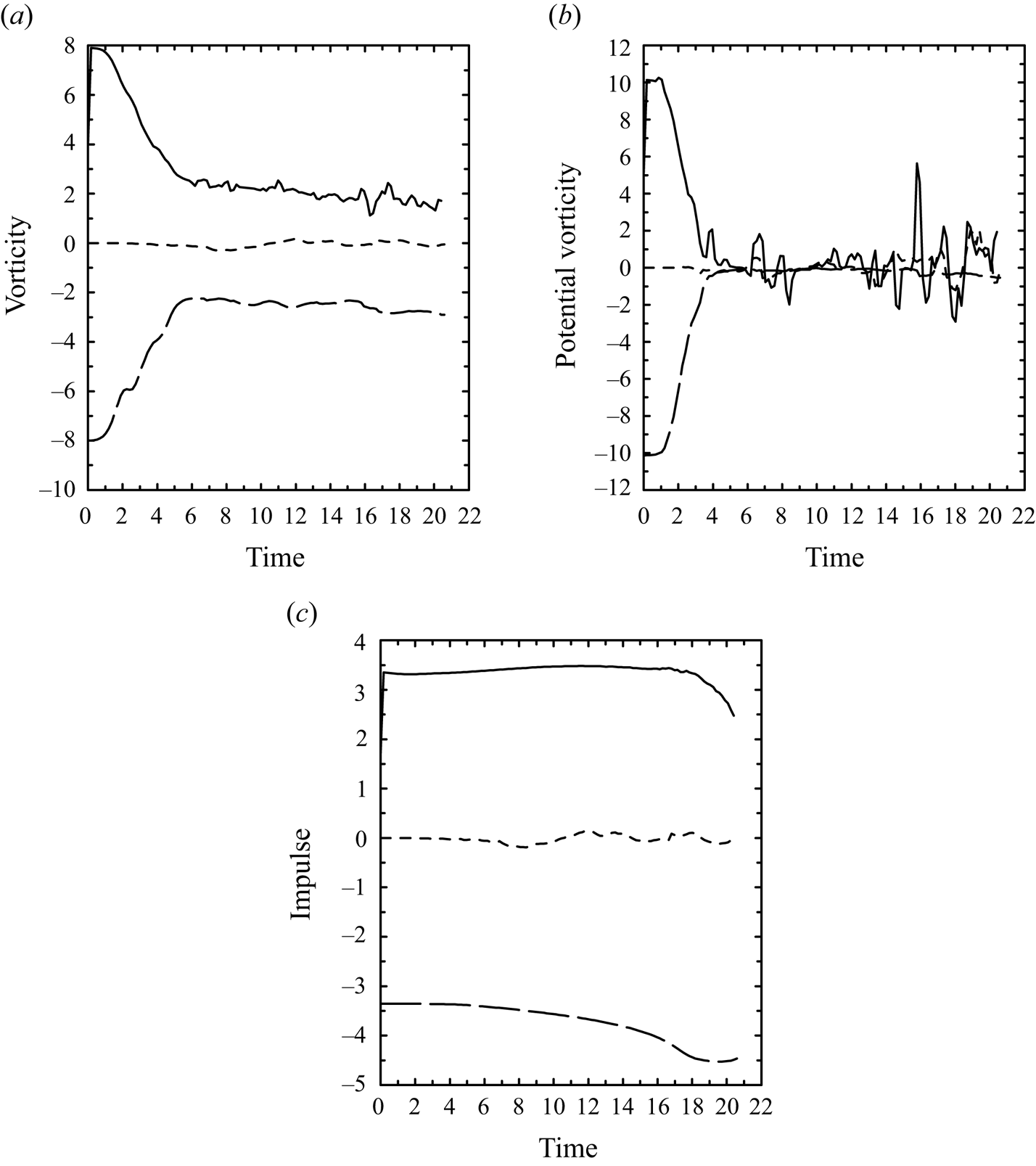
The integrated budgets of (a) the vorticity,  $\varGamma$, (b) the potential vorticity,
 $Q$, and (c) the impulse budget,
 $P$. The total tendency (solid) and the axisymmetric (long dash) and non-axisymmetric (short dash) forcings are shown. For clarity, the signs for the two forcing terms are flipped so that the sum of the curves should vanish.
Time series of the propagation efficiency factor,  ${\tilde {v}}_z$, diagnosed from (4.7).
With the similarity regime established by  $t= 3.4$, the relative contribution of
 $\bar {G}$ (d) to the
 $\bar {\zeta }$ budget, is about
 $1/3$ of the magnitude of both the local tendency,
 $\partial \bar {\zeta }/\partial t$ (a), and the advection,
 $s{\bar {\boldsymbol {v}}}\boldsymbol {\cdot } \boldsymbol {\nabla }(\bar {\zeta }/s)$ (b), as seen by comparing the three fields in figure 3(a,b,d). On the other hand, the buoyancy forcing,
 $-\partial \bar {b}/\partial s$ (c), is characterized by a sharp gradient along the thermal boundary during the early stages of evolution by initiating the simulation with a spherically homogeneous buoyant bubble. This sharp gradient gradually decreases with time due to SGS mixing, as seen in figure 3(c).
At a later stage (say,  $t \simeq 10$),
 $\bar G$ becomes as large as the other terms, apart from the buoyancy forcing, which is less than 1 % of other terms in magnitude. This result suggests that in the later stage of the simulation, the three-dimensionality of the dynamics plays a crucial role in the local dynamics. In summary, the contribution of the non-axisymmetric forcing,
 $\bar {G}$, to the vorticity budget is fairly significant, although the forcing is dominated by small-scale structures (much smaller than the scale of the thermal) as seen in figure 3(d). However, as will be demonstrated in the following, these structures contribute little to the volume-integrated budgets of the azimuthal vorticity.
4. Vortex-dynamics based analysis
4.1. Volume-integrated equations
To examine the vorticity dynamics of the thermal vortex ring in a concise manner, following Yano (Reference Yano2023), we focus on volume integrals of the vorticity with weights,  $s^n$, where
 $n$ is an integer exponent factor; here
 $n = 0, -1, 1$. The first two correspond to the volume integrals,
 $\varGamma$ and
 $Q$, of the vorticity,
 $\zeta$, and the potential vorticity,
 $\zeta /s$, respectively, and the third is the impulse,
 $P$. We perform the integrals over the full domain of the system. Noting that the volume element in axisymmetric cylindrical coordinates is given by
 ${\rm d}^3 r = s \,{\rm d}s \,{\rm d}z$, these volume integral quantities are defined by
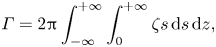 \begin{gather} \varGamma = 2{\rm \pi} \int^{+\infty}_{-\infty}\int^{+\infty}_0 \zeta s \,{\rm d}s \,{\rm d}z, \end{gather}
 \begin{gather}Q = 2{\rm \pi} \int^{+\infty}_{-\infty}\int^{+\infty}_0 \frac{\zeta}{s} s \,{\rm d}s \,{\rm d}z, \end{gather}
 \begin{gather}P = {\rm \pi}\int^{+\infty}_{-\infty}\int^{+\infty}_0 (s\zeta) s \,{\rm d}s \,{\rm d}z. \end{gather}
Keep in mind that these integrals are replaced by those over the simulation domain in the actual analysis.
These volume-integrated variables are governed by
 \begin{gather} \frac{{\rm d} \varGamma}{{\rm d}t} = 2{\rm \pi} \int^{+\infty}_{-\infty}\int^{+\infty}_0 (\bar{b} +\bar{u}_s\bar{\zeta}) s \,{\rm d}s \,{\rm d}z+ 2{\rm \pi} \int^{+\infty}_{-\infty}\int^{+\infty}_0 \overline{u_s^{\prime} \zeta^{\prime}} s \,{\rm d}s \,{\rm d}z, \end{gather}
 \begin{gather}\frac{{\rm d}Q}{{\rm d}t} =\left. 2{\rm \pi} \int^{+\infty}_{-\infty} b\right\vert_{s=0} \,{\rm d}z+ 2{\rm \pi} \int^{+\infty}_{-\infty}\int^{+\infty}_0 \frac{\overline{u_s^{\prime} \zeta^{\prime}_s}}{s} s \,{\rm d}s \,{\rm d}z, \end{gather}
 \begin{gather}\frac{{\rm d} P}{{\rm d}t} = 2{\rm \pi} \int^{+\infty}_{-\infty}\int^{+\infty}_0 \bar{b} s\,{\rm d}s \,{\rm d}z +{\rm \pi} \int^{+\infty}_{-\infty}\int^{+\infty}_0 (2s \overline{u_s^{\prime} \zeta^{\prime}} -\overline{u_{\varphi}^{\prime} \zeta^{\prime}_s} ) \,{\rm d}s \,{\rm d}z . \end{gather}
Here, on the right-hand side of (4.2a–c), the first and second integrals are, respectively, contributions of the axisymmetric and non-axisymmetric components to the tendency.
The total tendency on the left-hand side as well as the axisymmetric and non-axisymmtric tendency components on the right-hand side are plotted in figure 4 for the integrated vorticity and potential vorticity,  $\varGamma$ (a),
 $Q$ (b), and the impulse,
 $P$ (c). The total tendency (left-hand side of (4.2a–c), solid curves) is well balanced with the tendency due to the axisymmetric components (first term on the right-hand side of (4.2a–c), long-dashed curves). Note that the term involving
 $\bar {u}_s\bar {\zeta }$ in the mean forcing of
 $\varGamma$ is negligible compared with that of the buoyancy, as later explicitly demonstrated in section 4.3 by the small magnitude of parameter
 $K$ in figure 6(c) later.
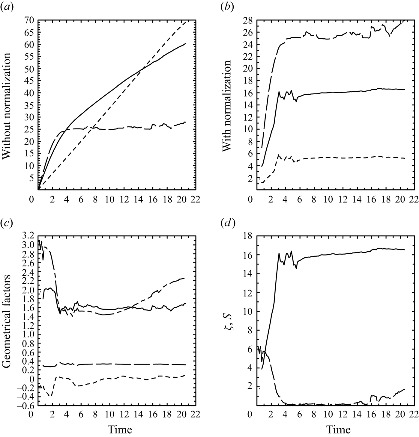
Time series of: (a)  $\varGamma$ (solid),
 $Q$ (long dash) and
 $P$ (short dash), as defined by (4.1a–c); (b) the same as (a), but with the normalizations of these quantities to give
 $\varGamma /R = \zeta _0$ (solid),
 $Q =Z\zeta _0$ (long dash) and
 $P/R^2\gamma \zeta _0$ (short dash); (c) geometrical factors,
 $Z$ (solid),
 $\gamma$ (long dash),
 $K$ (short dash) and
 $B$ (chain dash); (d)
 $\zeta _0$ (solid) and
 $S$ (long dash).
The contribution of the non-axisymmetric components (second term on the right-hand side of (4.2a–c), short-dashed curves) is fairly small. Here, the terms on the right-hand side are shown with signs reversed so that the sum of these three curves would vanish if the balance was exact. The total tendency, directly diagnosed by the left-hand side of the equation, is slightly noisier than the diagnosed right-hand side terms due to the fact that it is diagnosed by a centred difference from the output data stored at a frequency of  $\Delta t =0.1715$, rather than being an instantaneous tendency.
Over the last stage of the simulation, say  $t > 15$, the estimated total forcings (right-hand side) tend to be larger than the actual tendencies (left-hand side). We suspect that the imbalance increases with time owing to an increasing role of SGS mixing at a later stage of the simulation, as also suggested by fine-broken spatial structures of the vorticity-budget terms seen in the later stage of the simulation (not shown).
4.2. Propagation efficiency factor
Based on the fact that contributions of the non-axisymmetric terms are small for all three integrated variables,  $\varGamma$,
 $Q$ and
 $P$, we will neglect those contributions in the following and instead focus on the axisymmetric dynamics of the system. From now on, we will also refer to the azimuthally averaged azimuthal vorticity,
 $\bar {\zeta }$, and buoyancy,
 $\bar {b}$, as simply the vorticity and buoyancy, respectively.
To describe the time evolution of the system (4.2a–c) in a more concise manner, following Yano (Reference Yano2023), we separate the evolution of the vorticity,  $\zeta$, into the components,
 $\zeta _0$, measuring the intensity of the vorticity, and,
 $\tilde {\zeta }$, representing its spatial structure. Thus,
 \begin{equation} \bar{\zeta}(s, z) = \frac{\zeta_0 }{ R^2}{\tilde{\zeta}}(\xi, \eta), \end{equation}
in which the intensity,  $\zeta _0$, is defined in units of the circulation and rescaled by a measure,
 $R$, of the size of the vortex ring. We also separate the buoyancy,
 $\bar {b}$, in the same manner with equivalent notations:
 \begin{equation} \bar{b}(s, z) = b_0{\tilde{b}}(\xi, \eta) . \end{equation}
The vortex and buoyancy distributions are normalized by
 \begin{gather} 2{\rm \pi} \int^{+\infty}_{-\infty}\int^{+\infty}_0 {\tilde \zeta}(\xi, \eta) \xi \,{\rm d}\xi \,{\rm d}\eta = 1, \end{gather}
 \begin{gather}2{\rm \pi} \int^{+\infty}_{-\infty}\int^{+\infty}_0 {\tilde b}(\xi, \eta) \xi \,{\rm d}\xi \,{\rm d}\eta = 1. \end{gather}
Here,  $(\xi, \eta ) = (s/R, z/R)$ are the rescaled coordinates. As a result of the normalizations (4.4a,b), the axisymmetric generation rate of the potential tendency (first term on the right-hand side of (4.2c)) becomes
 \begin{equation} F \equiv 2{\rm \pi} \int^{+\infty}_{-\infty}\int^{+\infty}_0 \bar{b}s \,{\rm d}s \,{\rm d}z = R^3 b_0 . \end{equation}
Recall that the simulation of MJY was initialized with a homogeneous buoyant bubble with  $b_0 = 1$ in a sphere with a unit radius,
 $R_0 =1$, and the evolution of the equivalent radius,
 $R_0$, giving the same volume as the simulated thermal, is tracked. Note that the equivalent radius defined in this manner is related to the vortex-ring size,
 $R$, introduced here by
 \begin{equation} R^3 = \frac{4{\rm \pi}}{3}R_0^3, \end{equation}
and thus, the initial vortex-ring size is  $R = (4{\rm \pi} /3)^{1/3} \simeq 1.6$. Also note that with the lack of a buoyancy source in this simulation, the volume-integrated buoyancy is conserved with time, and
 $F = 4{\rm \pi} /3$. Here, it may be worthwhile to note that the assumption of constant forcing also relies on the assumption that the buoyancy remains confined within the vortex ring, i.e. buoyancy is not detrained into the environment. The assumption of little detrainment for dry thermal vortex rings is well supported by previous numerical simulations (e.g. Lecoanet & Jeevanjee Reference Lecoanet and Jeevanjee2019).
As explicitly shown by Yano (Reference Yano2023), it follows from the normalization (4.3a) that the propagation speed,  $\bar w$, of a vortex ring is
 \begin{equation} \bar{w} = \frac{\zeta_0 }{ R}{\tilde{v}}_z , \end{equation}
where  $\zeta _0$ and
 $R$ are measures of the vortex-ring intensity and size introduced in (4.3a), and
 ${\tilde {v}}_z$ is a propagation efficiency factor defined solely in terms of the vorticity distribution, as seen by (30a) of Yano (Reference Yano2023). Thus, the parameter,
 ${\tilde {v}}_z$, becomes constant with time in the similarity regime, because the vorticity distribution, after normalizing by the scale,
 $R$, must be constant with time in this regime. Thus, the similarity regime in the simulation of MJY can be identified by plotting
 ${\tilde {v}}_z$, diagnosed from (4.7), as in figure 5;
 ${\tilde {v}}_z$ is fairly close to a constant after the initial spin-up period of
 $t=0\unicode{x2013}3$.
4.3. Analysis under the axisymmetric assumption
By substituting (4.4a,b) into (4.1a–c), we find that
 \begin{gather} \varGamma = R\zeta_0, \end{gather}
 \begin{gather}Q = Z\zeta_0 , \end{gather}
 \begin{gather}P = \gamma \zeta_0 R^2 , \end{gather}
where  $Z$ and
 $\gamma$ are geometrical factors defined by
 \begin{gather} Z = 2{\rm \pi} \int^{+\infty}_{-\infty}\int^{+\infty}_0 \frac{\tilde\zeta}{\xi} \xi \,{\rm d}\xi \,{\rm d}\eta , \end{gather}
 \begin{gather}\gamma = {\rm \pi}\int^{+\infty}_{-\infty}\int^{+\infty}_0 (\xi \tilde\zeta) \xi \,{\rm d}\xi \,{\rm d}\eta . \end{gather}
An advantage of this reduction is that the problem of the time evolution of the three integrated variables,  $\varGamma$,
 $Q$ and
 $P$, is reduced to that of a single variable, the vortex-intensity measure,
 $\zeta _0$, when the evolution of the vortex-ring size,
 $R$, as well as that of the geometrical factors,
 $Z$ and
 $\gamma$, can be obtained by separate considerations.
Substitution of (4.4a,b) into the right-hand sides of (4.2a–c) leads to
 \begin{gather} \frac{{\rm d}\varGamma}{{\rm d}t} = R^2 B b_0 + \frac{K}{R}\zeta_0^2, \end{gather}
 \begin{gather}\frac{{\rm d}Q}{{\rm d}t} = Rb_0 S, \end{gather}
 \begin{gather}\frac{{\rm d}P}{{\rm d}t} = R^3b_0, \end{gather}
where
 \begin{gather} B = 2{\rm \pi}\int^{+\infty}_{-\infty}\int^{+\infty}_0 \tilde{b}\,{\rm d}\xi \,{\rm d}\eta , \end{gather}
 \begin{gather}K = 2{\rm \pi}\int^{+\infty}_{-\infty}\int^{+\infty}_0 \tilde{u}_s\tilde{\zeta}\,{\rm d}\xi \,{\rm d}\eta \end{gather}
are additional geometrical factors, and
 \begin{equation} S = 2{\rm \pi} \left.\int^{+\infty}_{-\infty}\tilde{b} \right\vert_{\xi=0}\,{\rm d}\eta \end{equation}
is an efficiency factor for the generation of integrated potential vorticity,  $Q$. Note that
 $K$ measures the deviation of the vorticity distribution from symmetry around the vortex-ring equatorial plane,
 $z=0$.
By further substituting (4.8a–c) into the left-hand sides of (4.10a–c), we obtain
 \begin{gather} R{\dot{\zeta}_0} + {\dot{R}}\zeta_0 = \frac{FB}{R} + \frac{K\zeta_0^2}{R} , \end{gather}
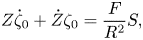 \begin{gather}Z{\dot{\zeta}_0}+{\dot{Z}}\zeta_0 = \frac{F}{R^2} S , \end{gather}
 \begin{gather}\gamma{\dot{\zeta}_0}R^2+{\dot{\gamma}}\zeta_0R^2+2\gamma\zeta_0R{\dot{R}} = F . \end{gather}
Here, we have also used the relation  $F = R^3 b_0$ to eliminate the buoyancy intensity,
 $b_0$, from the equations.
Equations (4.12a–c) form a set of prognostic equations for the vorticity intensity,  $\zeta _0$, vortex-ring size,
 $R$, and the geometrical factors,
 $Z$ and
 $\gamma$, under given forcings characterized by the parameters
 $F$ and
 $S$, along with the additional geometrical factors
 $B$ and
 $K$. However, the number of equations (three) is less than the number of variables to be predicted (four). Furthermore, to close the system, the time evolution of the forcing parameters,
 $S$,
 $B$ and
 $K$, must also be prescribed. Recall that the volume-integrated buoyancy forcing,
 $F$, is constant in time since there is no diabatic heating in the simulation.
In seeking insight to proceed further, we first examine the time evolution of these variables and parameters in the numerical simulation (figure 6). Thus, we analyse (a) the time series of  $\varGamma$ (solid),
 $Q$ (long dash) and
 $P$ (short dash); (b) the same as (a), but normalized by the vortex-ring size,
 $R$,
 $\varGamma /R = \zeta _0$ (solid),
 $Q =Z\zeta _0$ (long dash) and
 $P/R^2\gamma \zeta _0$ (short dash). We also analyse the time series of the geometrical factors,
 $Z$ (solid, (4.9a)),
 $\gamma$ (long dash, (4.9b)),
 $B$ (chain dash, (4.11a)) and
 $K$ (short dash, (4.11b)), which are shown in (c), and those of the vorticity intensity (solid),
 $\zeta _0$, as introduced in (4.8a–c), and the buoyancy source,
 $S$ (long dash, (4.11c)) in (d).
It is seen in figure 6(c) that the two geometrical factors,  $Z$ and
 $\gamma$, remain approximately constant throughout the simulation, apart from a sudden decrease of
 $Z$ by about
 $1/4$ at the end of the initial spin-up period,
 $t=0\unicode{x2013}3$. Constancies of these two factors are also inferred from the fact that the normalized volume-integral measures of the vorticity,
 $\varGamma /R$,
 $Q$ and
 $P/R^2$, shown in figure 6(b), overall evolve in parallel and, thus, ratios of these quantities are approximately constant. Thus, the time derivatives of
 $Z$ and
 $\gamma$ may be neglected in (4.12b,c). The measure of asymmetry,
 $K$, remains small (i.e.
 $|K| \ll Z$) for the whole period so that it may also be dropped in (4.12a). After these approximations, (4.12a–c) reduce to
 \begin{gather} R{\dot{\zeta}_0} + {\dot{R}}\zeta_0 = \frac{FB}{R}, \end{gather}
 \begin{gather}Z{\dot{\zeta}_0} = \frac{F}{R^2} S, \end{gather}
 \begin{gather}\gamma{\dot{\zeta}_0}R^2+2\gamma\zeta_0R{\dot{R}} = F . \end{gather}
4.4. Initial spin-up evolution
As already noted, the present system evolves through two regimes: the initial spin-up period ( $t=0\unicode{x2013}3$) and the similarity regime (
 $t > 3$). In time series of the normalized volume-integrated measures,
 $\varGamma /R$,
 $Q$ and
 $P/R^2$ (figure 6b), the initial spin-up period is characterized by their increase with time. The dynamics of the similarity regime are already relatively well understood (Scorer Reference Scorer1957; Turner Reference Turner1957; Yano Reference Yano2023), and have also been closely examined for the present simulation in MJY. Thus, the following will focus on the evolution during the initial spin-up period.
The main feature of the initial spin-up period is that the vortex circulation develops (i.e.  $\dot {\zeta }_0 >0$), which is dictated by the buoyancy (
 $S> 0$) along the vortex-ring axis (
 $s = 0$), as shown in figure 6(d); (4.13b) describes this process. Thus, a closed description of the initial spin-up period becomes possible in the phase space of
 $(S, \zeta _0)$ (cf. figure 7a) with an additional prognostic equation for the buoyancy source along the vortex-ring axis,
 $s=0$. This equation is introduced heuristically in the following manner.
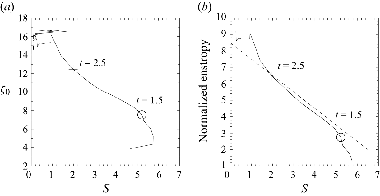
Evolution of the system in phase space of (a)  $(S, \zeta _0)$ and (b)
 $(S, \alpha Z\zeta _0^2/2F)$. The positions at
 $t=1.5$ and
 $2.5$ are marked by a circle and
 $+$ sign, respectively. A theoretical prediction based on (4.18) is also added as a dashed straight line.
Here, the buoyancy source along the vortex-ring axis ( $s=0$) is ventilated by advection associated with the vortex-ring circulation. This process is most simply described as a damping process with a characteristic time scale,
 $\tau$:
 \begin{equation} \dot{S} ={-}\frac{S}{\tau}. \end{equation}
Here, the damping time scale,  $\tau$, is expected to be controlled by advection, thus,
 \begin{equation} \tau \sim \frac{R}{u_0} = \frac{R^2}{\zeta_0}. \end{equation}
The second equality is obtained by setting the velocity scale to be  $u_0 = \zeta _0/R$. Note that as a result, the characteristic time scale,
 $\tau$, introduced in (4.14a), becomes time dependent based on the more explicit definition given by (4.14b). By substituting (4.14b) into (4.14a), we obtain
 \begin{equation} \dot S ={-}\frac{\alpha \zeta_0}{R^2}S, \end{equation}
where  $\alpha$ is a constant.
Thus, (4.13b) and (4.15) provide a closed description of the initial spin-up period. Noting that the right-hand sides of both equations share the same factor,  $S/R^2$, we can write them as
 \begin{equation} \frac{S}{R^2} = \frac{Z}{F}\dot{\zeta}_0 ={-}\frac{\dot{S}}{\alpha \zeta_0}, \end{equation}
which can be rearranged to give
 \begin{equation} \frac{\alpha Z}{F}\zeta_0\dot{\zeta}_0 +\dot{S}=0. \end{equation}
Assuming that  $\alpha Z/F$ is approximately constant, the last expression can be integrated to give
 \begin{equation} \frac{\alpha Z}{2F}\zeta_0^2 + S= {\rm const.} \end{equation}
To examine the validity of the solution (4.18), figure 7(b) plots the normalized enstrophy,  $\alpha Z\zeta _0^2/2F$, against
 $S$; this relation is close to a straight line over
 $t=1.5\unicode{x2013}2.5$, and to a lesser extent over a longer time span. A good fit is found with
 $\alpha = 0.2$, as marked by the dashed straight line. More precisely, towards
 $t=3$, the vorticity intensity,
 $\zeta _0$, shoots up briefly, then decreases towards
 $t =4$, as also seen in figure 6(d). Furthermore, by comparing (a,b) in figure 7, it is apparent that the time dependence of the factor,
 $Z/F$, needs to be retained in order to accurately describe the linear dependence of the normalized enstrophy,
 $Z\zeta _0^2/2F$, on the buoyancy source along the vortex-ring axis (
 $s=0$) in a parametric manner, although it is neglected in the derivation. Overall, we conclude that the agreement is satisfactory considering the heuristic nature of this model.
4.5. Buoyancy equation
The consistency of the empirically derived buoyancy equation (4.15) can be directly verified by analysing the buoyancy budget:
 \begin{equation} \frac{\partial \bar{b}}{\partial t} ={-}\boldsymbol{\nabla}\boldsymbol{\cdot}\overline{b{\boldsymbol{v}}}. \end{equation}
Here, we retain contributions of the non-axisymmetric components on the right-hand side. By vertically integrating this equation along the vortex-ring axis ( $s=0$), we obtain
 \begin{equation} \left.\frac{\partial }{\partial t}\int^{+\infty}_{-\infty}\bar{b}\right\vert_{s=0} \,{\rm d}z = \left.-\int^{+\infty}_{-\infty}\left[\frac{1}{s}\frac{\partial}{\partial s} s\overline{bu_s}\right]\right\vert_{s=0}\,{\rm d}z . \end{equation}
Comparing the left-hand side with the definition (4.11c) of  $S$, we find that
 \begin{equation} -\!\frac{1}{2{\rm \pi}}\frac{F}{R^2}\dot{S} = \int^{+\infty}_{-\infty}\left.\left[\frac{1}{s}\frac{\partial}{\partial s} s \bar{b}\bar{u}_s\right]\right\vert_{s=0}\,{\rm d}z +\left.\int^{+\infty}_{-\infty}\left[\frac{1}{s}\frac{\partial}{\partial s} s\overline{b^{\prime}u_s^{\prime}}\right]\right\vert_{s=0}\,{\rm d}z, \end{equation}
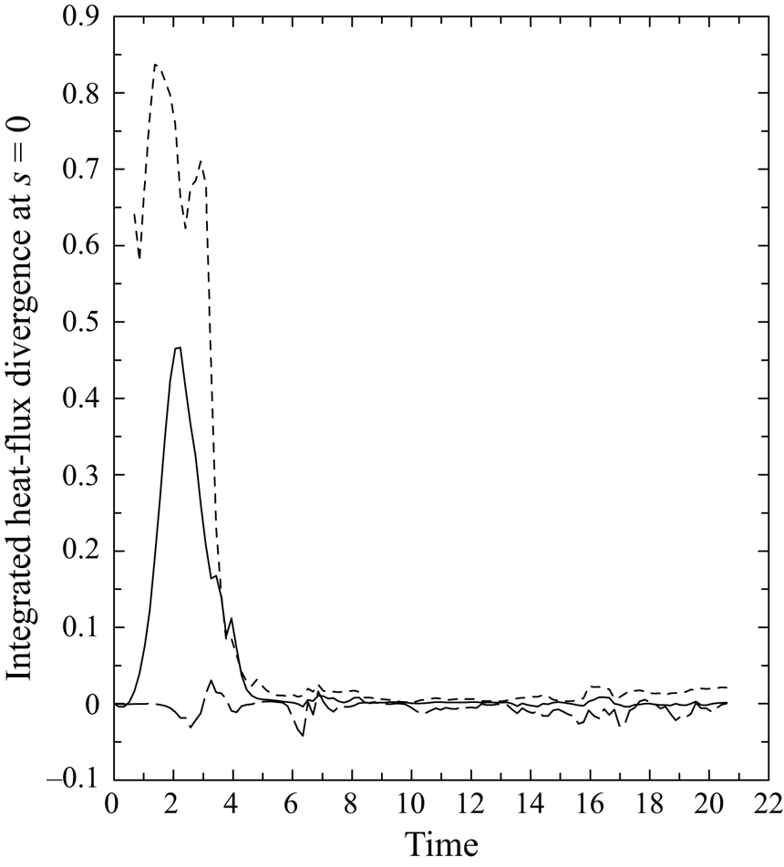
where the right-hand side is divided into the contributions by axisymmetric and non-axisymmetric components in the first and second terms, respectively. These two terms of the heat-flux divergence are plotted in figure 8 as solid and long-dashed curves, respectively; again, it is seen that the contribution (long dash) of the non-axisymmetric components is overall small compared with that of the axisymmetric components (solid) during the spin-up period. Furthermore, the estimate of the heat-flux divergence based on the empirical prognostic equation (4.15) is shown by the short-dashed curve. It reproduces the overall behaviour of the direct estimate (solid), with the remaining discrepancy attributed to the SGS mixing in simulation of MJY.
The flux-divergence terms controlling the evolution of the buoyancy integrated along the  $z$ axis: the term due to the axisymmetric flow (solid), and the contribution of the non-axisymmetric flow (long dash), corresponding to the first and second terms on the right-hand side and the term on the left-hand side in (4.21). Further added is the estimate based on the heuristic model,
 $-(1/2{\rm \pi} )F/R^2\dot {S}$ (short dash), in which
 $\dot {S}$ is estimated by the right-hand side of (4.15).
4.6. Evolution over the similarity regime
At the end of the initial spin-up period, the buoyancy source along the vortex-ring axis,  $s=0$, is fairly small, and it no longer increases the vorticity intensity,
 $\zeta _0$, in any substantial manner afterwards. This marks the beginning of the similarity regime (
 $t > 4$). In the similarity regime, therefore,
 $\dot {\zeta }_0$ can be dropped in (4.13a,c). As a result, they reduce to prognostic equations for the vortex-ring size,
 $R$. Both equations lead to solutions with tendencies,
 $R \sim t^{1/2}$, as expected from the similarity theory as shown in Yano (Reference Yano2023).
Furthermore, constant factors in solutions obtained from both equations must also be identical, because these two equations must predict the same evolution in a mutually consistent manner. This consistency condition is given by
 \begin{equation} 2\gamma B = 1. \end{equation}
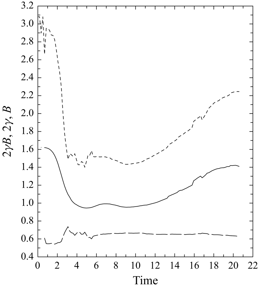
This condition (4.22) is verified in figure 9; the condition is satisfied fairly well over  $t=3\unicode{x2013}13$ with the value of
 $2\gamma B$ fairly close to unity (solid curve). Before and after this period, the constant is larger than unity, with an increasing tendency for
 $t > 13$. This deviation tendency for both periods is explained by larger values of
 $B$ (short dash) over those periods. These larger values of
 $B$, in turn, are explained by the buoyancy being concentrated in the vortex-ring core during the initial spin-up period as well as towards the end of the simulation (cf. figure 6 of MJY). In contrast, the geometrical factor
 $\gamma$ (long dash) remains fairly constant over the whole simulation period.
Time series of  $2\gamma B$ (solid), which is expected to be unity following the consistency condition (4.22), as well as two geometrical factors,
 $2\gamma$ (long dash) and
 $B$ (short dash).
5. Turbulent nature of the thermal vortex ring: two- vs three-dimensionality
The analysis so far suggests that the overall evolution of the thermal vortex ring simulated by MJY, such as the vorticity intensity,  $\zeta _0$, the size,
 $R$, as well as the buoyancy distribution,
 $\bar {b}$, can well be described in a closed form by the axisymmetric dynamics of the vorticity, although the impact of the non-axisymmetric eddies at local scales is non-negligible. These results further suggest that the dynamics of the thermal vortex ring may be understood in analogy with two-dimensional turbulence in terms of the axisymmetric flow. In the absence of non-axisymmetric flows, this analogy is valid apart from differences arising from the cylindrical geometry. In other words, axisymmetric flow differs from the common view of two-dimensional flow on a flat planar surface, yet the axisymmetric system here is described only by two coordinates,
 $s$ and
 $z$. Thus, under a standard terminology both in classical mechanics and dynamical-system studies, this system is unambiguously two dimensional (since non-axisymmetric eddies contribute little to overall evolution of the thermal vortex ring). Moreover, the governing equation system, as presented by (3.1a), is a close analogue to that for the vorticity equation on the plane, apart from some geometrical factors such as
 $1/s$ on the vorticity as well as the buoyancy forcing on the right-hand side. Thus, it is reasonable to expect that this system might behave like a two-dimensional flow to some extent, which is a key question posed in the present section.
The purpose of this section is to infer the extent of which present system can be interpreted as a two-dimensional flow. One may note that this perspective is oversimplified, because as we have already seen (especially in figure 3), the contributions of the non-axisymmetric components to the vorticity dynamics are not small locally. However, we have also found that when the vorticity budget is analysed in terms of the volume-integrated quantities, as in (4.2a–c), the nonlinear contributions of the symmetric components in turn are negligible (cf. figure 4).
5.1. Gross features
We first examine simple volume averages to infer the degree that the simulated system is two dimensional. In the following, we refer to the square of the velocity and buoyancy collectively as powers with the velocity squared referred to as kinetic energy later. For evaluating the velocity power, the velocity in the absolute space is used so that the mean vertical velocity (equal to minus the thermal vortex-ring velocity) in the moving frame that dominates at the far field is removed.
Naively, the simulated flow can be argued to be close to two dimensional if the flow is overall dominated by the axisymmetric component. To see this possibility, figure 10 plots the fractions of the total velocity and buoyancy powers explained by the axisymmetric components. Initially ( $t=0\unicode{x2013}2$), both fractions are fairly close to unity. The relative contribution from the axisymmetric component of velocity power even exceeds unity during this period, presumably due to noise generated by interpolating to the cylindrical coordinates. However, after the initial spin-up period (
 $t=0\unicode{x2013}4$), the fraction of the buoyancy power from the axisymmetric component rapidly drops below 0.75. On the other hand, the decrease of the velocity–power fraction is relatively gradual, and it remains above 0.95 throughout the simulation. Thus, the flow associated with the simulated thermal vortex is fairly axisymmetric in this respect.
Fraction of the total power explained by the axisymmetric component for the velocity (solid) and the buoyancy (long dash). Here, the velocity is defined in absolute space.
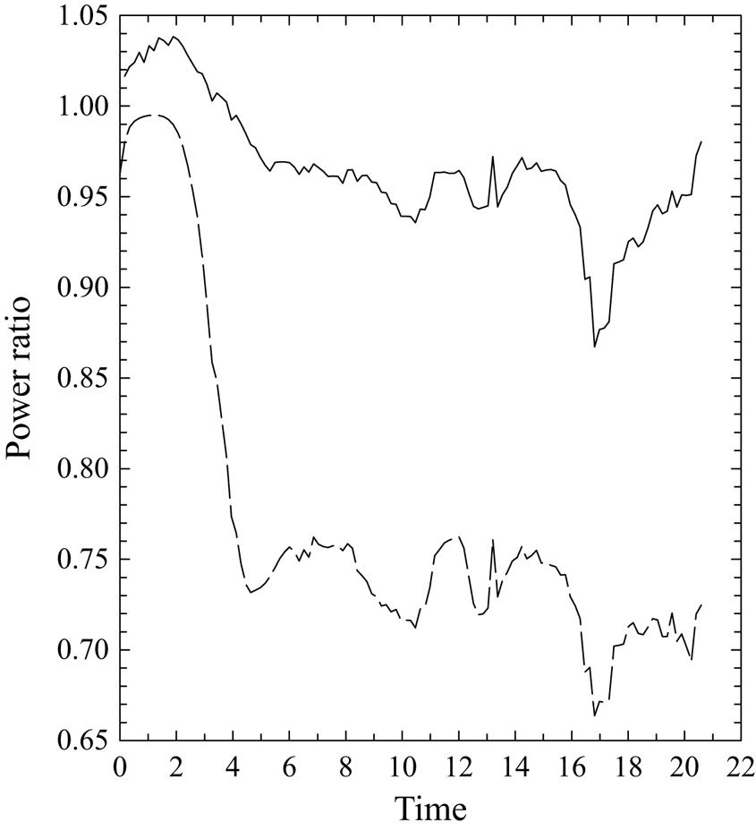
We also comment on the sudden drops followed by recovery over  $t=16\unicode{x2013}19$ seen for both variables in figure 10. A direct inspection identifies a transient, slight destabilization of the vortex-ring core noticeable in both the vorticity and buoyancy fields. Nevertheless, these dips are relatively weak in magnitude, with a slightly more prominent spike in figure 4(b) compared with that in figure 4(a). This time,
 $t \simeq 17$, is also when the deviation from the consistency condition (4.22) is apparent in figure 9.
5.2. Spectra
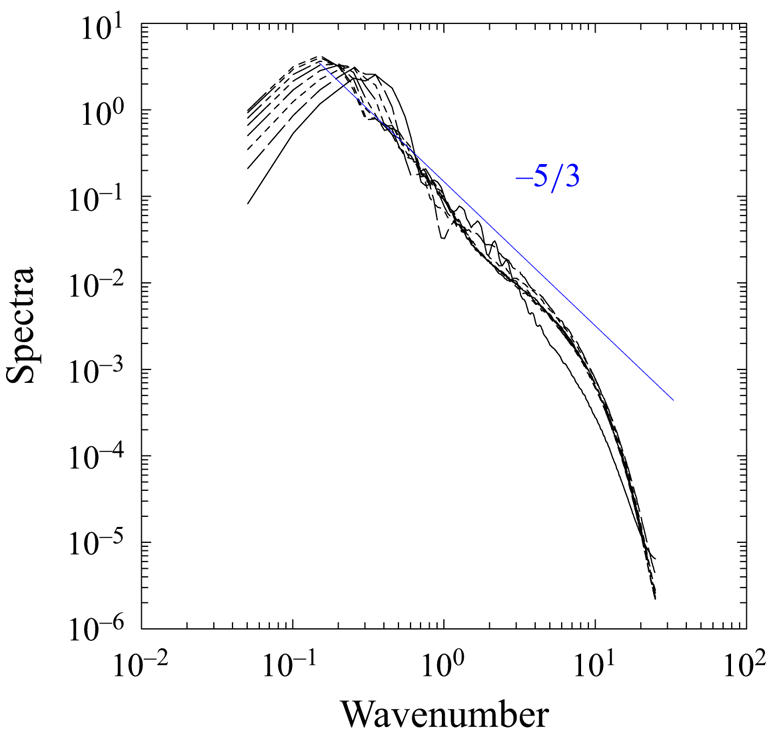
Another manner of assessing two-dimensionality of the simulated flow is to examine the power spectra of the velocity and buoyancy. In the following, we focus on the former, which we refer to as the kinetic energy. Direct evaluations of the spectra in the full three-dimensional space, after an initial spin-up period, leads to a power spectrum with an exponent close to  $-5/3$ (figure 11). We are inclined to interpret this as a signature that the simulated flow as a whole is consistent with three-dimensional turbulence. However, we also need to keep in mind that the
 $-5/3$ slope of the spectrum does not necessarily prove a system to be three-dimensional homogeneous turbulence. Two examples come to mind. First, under the standard theories for the two-dimensional turbulence, a
 $-5/3$ kinetic energy spectrum is expected for the inverse-cascade inertial subrange (Kraichnan Reference Kraichnan1967, Reference Kraichnan1971; Boffetta & Ecke Reference Boffetta and Ecke2012). Second, the atmospheric kinetic energy spectrum below a scale of
 $\sim$700 km is known to take a slope of
 $-5/3$ (Gage & Nastrom Reference Gage and Nastrom1986). However, the flow of this scale, typically referred to as stratified turbulence, is still considered quasi-two dimensional under hydrostatic balance (cf. Lindborg Reference Lindborg2006).
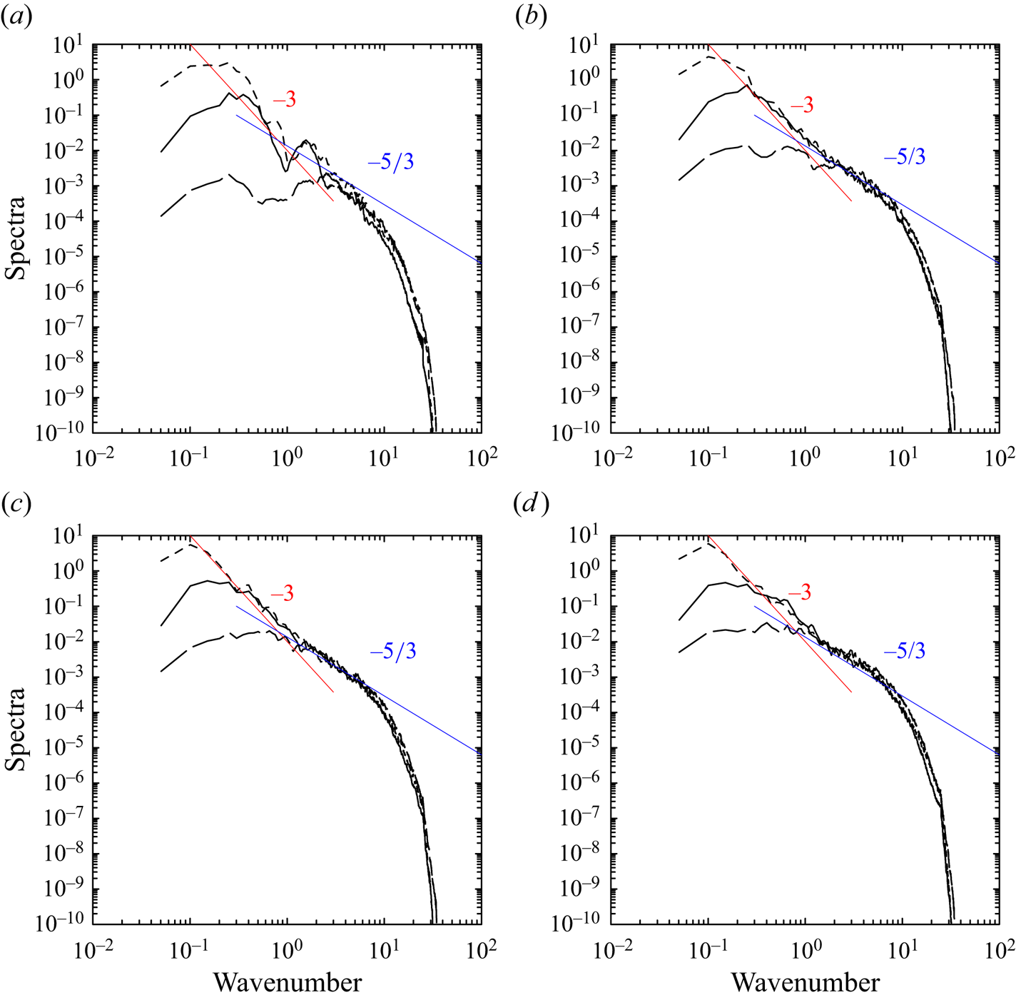
Power spectra of the kinetic energy of the system plotted from  $t=2.58$ to
 $20.1$ with a step of
 $2.58$ with the varying curves. The total power of spectra is normalized to unity. A slope for the power exponent of
 $-5/3$ is also marked in blue.
When the same spectra are evaluated after the azimuthally averaging of the velocity field, the slope of the spectra becomes much steeper and closer to a  $-3$ slope as expected for the forward enstrophy-cascade inertial subrange of two-dimensional turbulence. However, this result is misleading to conclude as a signature of the axisymmetric component to be two-dimensional turbulence; the obtained slope is more likely a consequence of the azimuthal averaging, which works as a low-pass filter.
It follows to analyse the spectra along different planes without applying any averaging. For this purpose, we evaluate the power spectra of velocity and buoyancy on the planes perpendicular to the  $x$,
 $y$ and
 $z$ axes in figures 12–14; these three planes are chosen to intersect the diagnosed centre of the vortex ring. This choice makes the
 $y$–
 $z$ and
 $x$–
 $z$ planes perpendicular to the azimuthal direction of the vortex ring, whereas the
 $x$–
 $y$ plane corresponds to the equatorial plane of the vortex ring. More specifically, the spectra shown in figure 12 are obtained by considering only the two-dimensional field on the
 $y$–
 $z$ plane, then performing a two-dimensional Fourier transform on the whole section (i.e. the whole domain). The total power is normalized to unity in the following presentation.
Power spectra calculated on the  $y$–
 $z$ plane containing the centre position of the vortex ring for the three velocity components:
 $x$ (solid),
 $y$ (long dash) and
 $z$ (short dash) directions at the time (a)
 $t=3.4$, (b)
 $t= 10.3$, (c)
 $t= 15.4$ and (d)
 $t= 19.7$. Spectra are normalized the total power to be unity. Slopes for power exponents of
 $-3$ (red) and
 $-5/3$ (blue) are also marked.

The same as figure 12 but on the  $x$–
 $z$ plane.
The same as figure 12 but on the  $x$–
 $y$ plane.
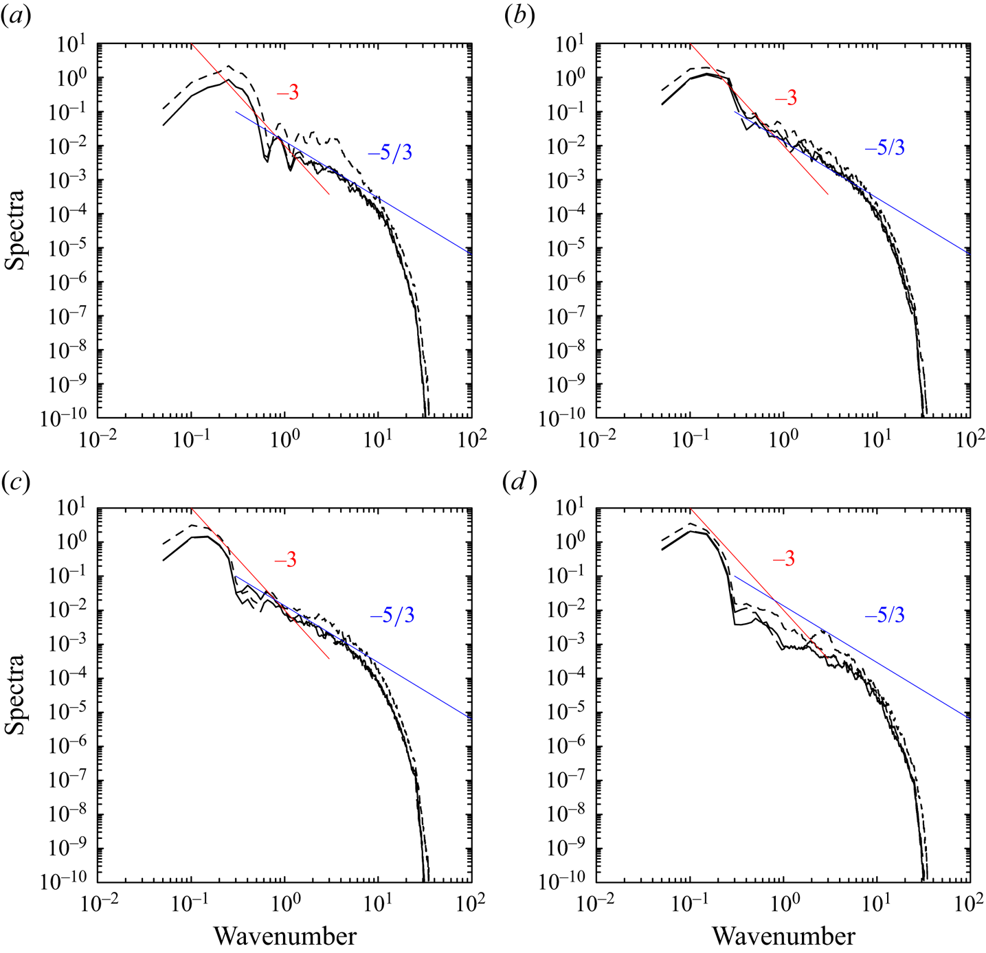
In all three plots, spectra are shown for  $t=3.4$ (a), 10.3 (b), 15.4 (c) and 19.7 (d), approximately corresponding to the times of the vertical cross-section plots shown in figure 6 of MJY. However, the spectrum shapes are rather surprisingly similar at all four times, although they correspond to qualitatively different phases in the vortex-ring evolution.
Spectra on the  $y$–
 $z$ and
 $x$–
 $z$ planes (figures 12–13) are distinguishably different from those on the
 $x$–
 $y$ plane (figure 14). In the former, moving to wavenumbers smaller than around
 $k=1\unicode{x2013}3$, the spectrum slope suddenly shifts from
 $-5/3$ at the smaller scales to
 $-3$ at the larger scales, which could be considered a signature of the forward enstrophy-cascade inertial subrange. This tendency is most prominent with the vertical velocity component, and to a lesser extent with the horizontal velocity component parallel to a given plane, i.e.
 $y$ and
 $x$ components in figures 12 and 13, respectively. The spectra of the velocity component perpendicular to the plane, on the other hand, decrease dramatically below this wavenumber range, suggesting that the flow at larger scales with
 $k < 1\unicode{x2013}3$ is quasi-two dimensional.
The overall shape of spectra for these two cross-sections is, probably coincidentally, strikingly similar to that observed for the atmosphere (Nastrom & Gage Reference Nastrom and Gage1985; Gage & Nastrom Reference Gage and Nastrom1986) with  $k=1\unicode{x2013}3$ roughly corresponding to the transition scale between the
 $-3$ and
 $-5/3$ slope regimes. Note that in the present system,
 $k=1$ corresponds to the initial radius of the buoyancy anomaly, which acts as a vorticity source throughout the simulation. Thus, it is natural to expect that this forcing scale
 $k\sim 1$ characterizes this system. The identified transition over
 $k=1\unicode{x2013}3$ is fairly close to this characteristic scale.
From these two sets of plots, we may conclude that the flows in directions perpendicular to the azimuthal direction of the vortex ring can be considered quasi-two dimensional for the scale range of, approximately,  $k=0\unicode{x2013}3$. This suggests that the evolution of the vortex ring over this scale range may be interpreted in analogy with a two-dimensional turbulence. On the other hand, over smaller scales (say,
 $k>3$) the flows are three dimensional, which is also suggested by nearly equal contributions of the three velocity components to the spectrum over this scale range.
In contrast, for the spectra on the  $x$–
 $y$ plane, all the three components have close to
 $-5/3$ slope for the full range of wavenumbers, although a gentle peak at
 $k \simeq 0.3$ with a noticeable deviation from this general tendency over
 $k=0\unicode{x2013}1$ is seen (figure 14); thus, the flow dissecting the equatorial plane of the vortex ring behaves more like three-dimensional turbulence.
6. Summary and discussion
A high-resolution simulation of a thermal vortex ring performed by using the large-eddy modelling set-up of Morrison et al. (Reference Morrison, Jeevanjee and Yano2022) has been analysed from a point of view of the vortex dynamics. The simulated thermal vortex-ring flow has substantial contributions from the non-azimuthal components, especially at smaller scales, as seen in the vorticity-budget analysis (figure 3). Moreover, the  $-5/3$ power spectrum for the kinetic energy obtained in full three-dimensional space (figure 11) as well as on planes perpendicular to the azimuthal direction (figure 14) appear to suggest the nature of the simulated flow as three-dimensional turbulence at smaller scales. Thus, one may also expect that the three-dimensional flow structure of the vortex ring plays a crucial role in the dynamics. However, from a point of view of the volume-integrated budgets of the vorticity and the potential vorticity as well as that of the impulse, the contributions of the non-axisymmetric eddies are insignificant; the overall evolution of the thermal vortex ring, including that of the vorticity intensity,
 $\zeta _0$, and the vortex-ring size,
 $R$, is well described solely in terms of the axisymmetric components of the flow.
The initial spin up of the vortex ring is controlled by the buoyancy integrated along the vertical axis of the ring. The buoyancy along the vertical-ring axis is ventilated out by the vortex-ring circulation generated as a consequence of the buoyancy anomaly itself. This ventilation rate is shown to be proportional to  $\zeta _0/R^2$ based on a simple dimensional argument. This leads to a simple closed description of the initial spin-up period of the vortex-ring evolution. This phenomenological description is supported by a buoyancy-budget analysis of the simulation. The prediction from this phenomenological model also agrees well with the numerically simulated evolution of the vortex spin up, as quantified by the vorticity intensity,
 $\zeta _0$.
We may observe two complementary aspects in deriving this phenomenological model. The first is the importance of directly examining the governing equations of the system explicitly, in the present case, both the vorticity and buoyancy equations. The second is, at the same time, obtaining an expression for the ventilation rate by a dimensional argument. In this manner, complementary use of these two approaches leads to a phenomenological model.
Geometrical factors remain overall constant with time over the whole evolution of the thermal vortex ring, including the initial spin-up period. Thus, one may interpret that these geometrical factors are fairly well defined by the initial conditions, and the subsequent evolution does not change the factors in any substantial manner. However, to reproduce the simulated evolution of the vorticity intensity,  $\zeta _0$, and the buoyancy source,
 $S$, at the initial spin-up period by the above phenomenological model, it is crucial to retain their time dependencies in a parametric manner (cf. § 4.4).
The dynamics of the thermal vortex ring may be overall interpreted in analogy of a two-dimensional turbulence, by focusing on the components of the flow perpendicular to the azimuthal direction. The  $-3$ slope of the energy spectra on the planes containing the vortex-ring axis supports this interpretation at larger scales. A remaining challenge is the extent to which the thermal vortex-ring dynamics can be understood in analogy with two-dimensional turbulence. Here, it is crucial to keep in mind that this analogy is not perfect, because the geometry of axisymmetric flows is different from the standard two-dimensional turbulence on a plane. For this reason, further investigations of axisymmetric turbulent flows would be required.
The present study has adopted a general framework for the analysis developed by Yano (Reference Yano2023) for describing the thermal vortex ring in terms of the vorticity budget. To fully close the formulation, additional equations for the geometrical factors are still required. The present study demonstrates that, nevertheless, the formulation by Yano (Reference Yano2023) can elucidate the dynamics of a thermal vortex-ring well, under the assumption that the geometrical factors are constant with time. Furthermore, being guided by the analysis results, a self-contained phenomenological description of the initial spin-up phase of the vortex ring has been obtained, as remarked above. In this manner, the present work showcases the combination of theory and numerical simulation for elucidating the fluid mechanics of thermal vortex rings.
Acknowledgements
J.-I.Y. acknowledges discussions with M. Wacławczyk on the two-dimensional turbulence.
Declaration of interests
The authors report no conflict of interest.


 Open access

