1 Introduction
The past three decades have undergone substantial progress in the development of layer-by-layer production methods via additive manufacturing (AM), or three-dimensional printing (3DP). Complex parts of various geometries are currently printable for a vast range of industrial applications, including metallic and organic parts (Miller et al. Reference Miller, Stevens, Yang, Baker, Nguyen, Cohen, Toro, Chen, Galie, Yu, Chaturvedi, Bhatia and Chen2012; Zheng et al. Reference Zheng, He, Gao and Liu2013; He, Xue & Fu Reference He, Xue and Fu2014; Hofmann et al. Reference Hofmann, Roberts, Otis, Kolodziejska, Dillon, Suh, Shapiro, Liu and Borgonia2014; Murphy & Atala Reference Murphy and Atala2014; Gibson, Rosen & Stucker Reference Gibson, Rosen and Stucker2015; Wegst. et al. Reference Wegst, Bai, Saiz, Tomsia and Ritchie2015; Mukherjee et al. Reference Mukherjee, Zuback, De and DebRoy2016; Yung et al. Reference Yung, Sun, Meng, Huang, Jin, Choy, Cai, Li, Ho, Yang and Wong2016; Chin et al. Reference Chin, Poh, Kohler, Compton, Hsu, Lau, Kim, Lee, Lee and Sia2017). Still, a number of undesirable effects hinder current production capabilities, including, among others, distortion and compositional changes (Mukherjee et al. Reference Mukherjee, Zuback, De and DebRoy2016), high surface roughness (Sames et al. Reference Sames, List, Pannala, Dehoff and Babu2016), corrugations due to wave motion and denudation (Matthews et al. Reference Matthews, Guss, Khairallah, Rubenchik, Depond and King2016). These effects are potentially controllable via the adjustment of material properties, temperature distribution, laser intensity and speed, geometry of the molten pool and various thermo-physical effects.
A main impediment in the prediction of these effects stems from the high temperature gradients near the laser source, which induce thermocapillary motion and the onset of Marangoni convection within the melt pool (Davis Reference Davis1987; Khairallah et al. Reference Khairallah, Anderson, Rubenchik and King2016; Sames et al. Reference Sames, List, Pannala, Dehoff and Babu2016). Microstructures of the grown solid are strongly affected by this flow (Kowal, Davis & Voorhees Reference Kowal, Davis and Voorhees2017b ) and compositional variations induce complex nonlinear pattern selection at the rapid solidification rates common to AM (Kowal, Altieri & Davis Reference Kowal, Altieri and Davis2017a ) and 3DP.
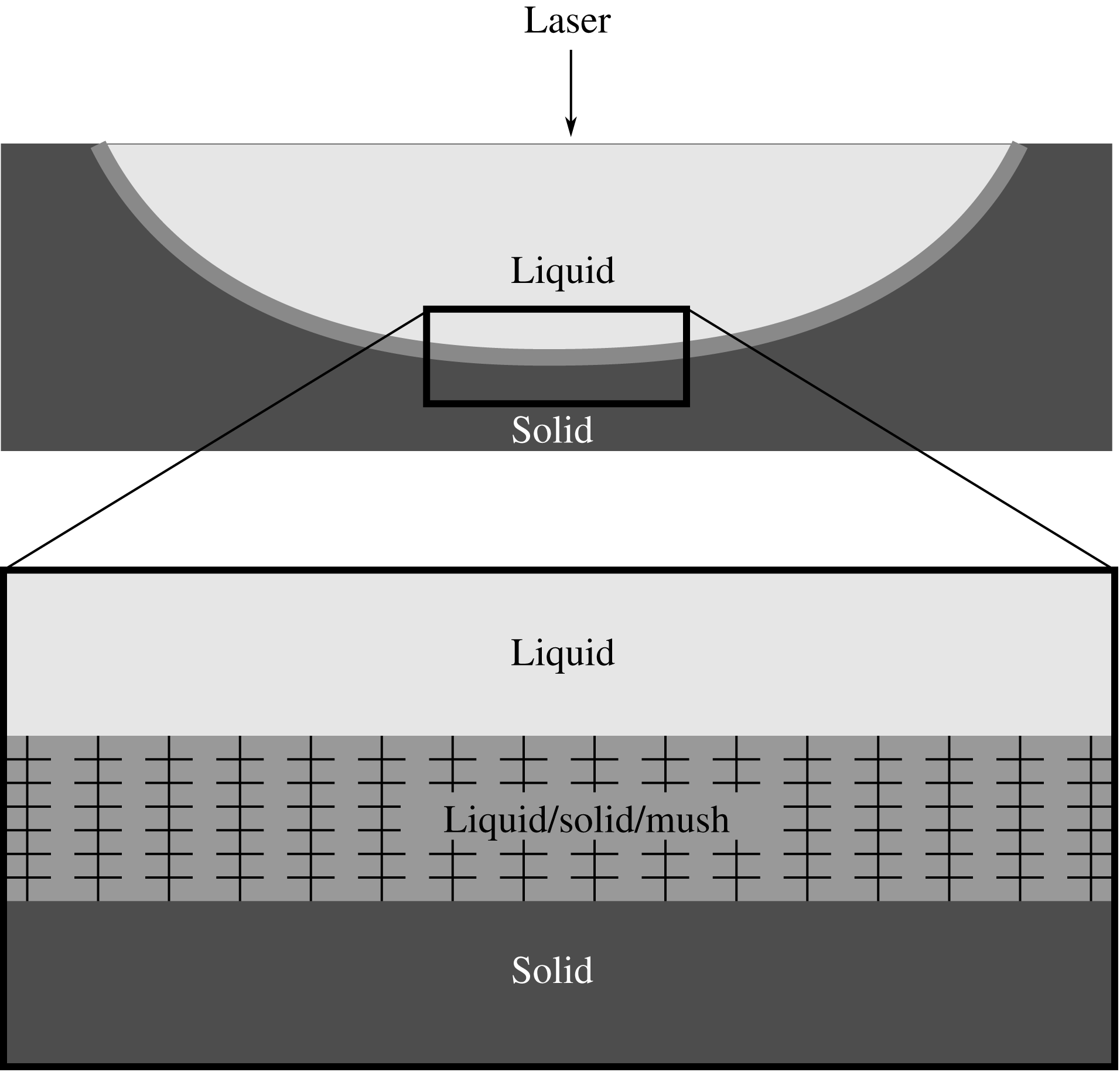
Schematic of the solidification of a liquid melt pool in additive manufacturing and an inset of the liquid/solid/mush layer.
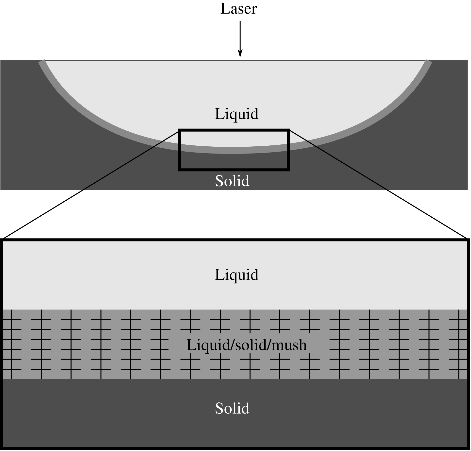
In the layer-by-layer production methods of AM, material is deposited upon a substrate, which subsequently melts under a moving laser heat source and tends to solidify by the ambient thermal field. This process is repeated continually, layer by layer, and the trajectories traversed determine the geometry of the finished product. Depending on the geometry and material properties of the desired product, as well as whether or not the same path is continually traversed, the substrate is either mostly solid, or mostly liquid. The schematic in figure 1 illustrates the geometry of the problem together with an inset that depicts a microscopic view of the substrate, or liquid/solid/mush layer that forms at the solid–liquid interface. The structure and composition of the substrate may vary on fine scales, much smaller than that of the liquid layer. In principle, one could use large-scale computational methods to describe the multi-layer flow, heat transfer and phase change present. This approach would give the details of the particular system but general insight into such systems is absent. Instead, we have ‘modelled’ the substrate as providing an effective slip to the top layer. Given the separation of scales, this provides a homogenized boundary condition on the scale of the layer of liquid, stemming from the homogenization of the mixture of solid and liquid. We are effectively averaging over the microstructure of the substrate to build in the effective slip experienced by the liquid layer into an effective slip coefficient
 $\unicode[STIX]{x1D6FD}^{-1}$
. The value of
 $\unicode[STIX]{x1D6FD}^{-1}$
spans the range from no slip to free slip. In effect, all of the properties of the substrate are incorporated in
 $\unicode[STIX]{x1D6FD}^{-1}$
. Given this model, we determine the effect of various substrates on the hydrothermal instabilities of the top layer, the preferred mode, the frequency of travel and the critical Marangoni number. In other areas of application, it is common for the bulk of thermocapillary flows to occur within a boundary layer near the upper, gas–liquid interface, especially for high-Marangoni-number flows (Cowley & Davis Reference Cowley and Davis1983). In these cases, the locus of the lower boundary of this layer is no longer a no-slip surface, and instead, partial slip is similarly to be expected.
Following Pearson (Reference Pearson1958), the onset of thermocapillary convection has been examined for a vast range of effects in various settings theoretically, for example, in two-dimensional slots of small aspect ratio (e.g. Sen & Davis Reference Sen and Davis1982) in thin liquid films at low capillary number (e.g. Smith & Davis Reference Smith and Davis1983a ,Reference Smith and Davis b ) and at high Marangoni number in a square cavity (Carpenter & Homsy Reference Carpenter and Homsy1990), as well as numerically (e.g. Takashima Reference Takashima1981; Zebib, Homsy & Meiburg Reference Zebib, Homsy and Meiburg1985; Chen & Hwu Reference Chen and Hwu1993; Mundrane, Xu & Zebib Reference Mundrane, Xu and Zebib1995; Xu & Zebib Reference Xu and Zebib1998; Hamed & Floryan Reference Hamed and Floryan2000; Nepomnyashchy, Simanovskii & Braverman Reference Nepomnyashchy, Simanovskii and Braverman2001; Shevtsova, Nepomnyashchy & Legros Reference Shevtsova, Nepomnyashchy and Legros2003; Saenz et al. Reference Saenz, Valluri, Sefiane, Karapetsas and Matar2013) and experimentally (e.g. Juel et al. Reference Juel, Mullin, Ben Hadid and Henry2001; Hof et al. Reference Hof, Juel, Zhao, Henry, Ben Hadid and Mullin2004) in numerous configurations. Four distinct modes of instability occur if the lower boundary obeys the no-slip condition, including two- and three-dimensional hydrothermal waves, longitudinal rolls and longitudinal travelling waves (Smith & Davis Reference Smith and Davis1983a ). In the current paper, we wish to examine how the selection of the preferred mode of instability changes under partial and free slip, and find another mode of instability that becomes preferable for larger slip parameters.
We begin by setting out our theoretical development and method of numerical solution in § 2. We discuss longitudinal instabilities, including longitudinal rolls and longitudinal travelling waves in § 3, two-dimensional hydrothermal waves in § 4 and oblique hydrothermal waves in § 5. We finalize with conclusions in § 6.
2 Theoretical development
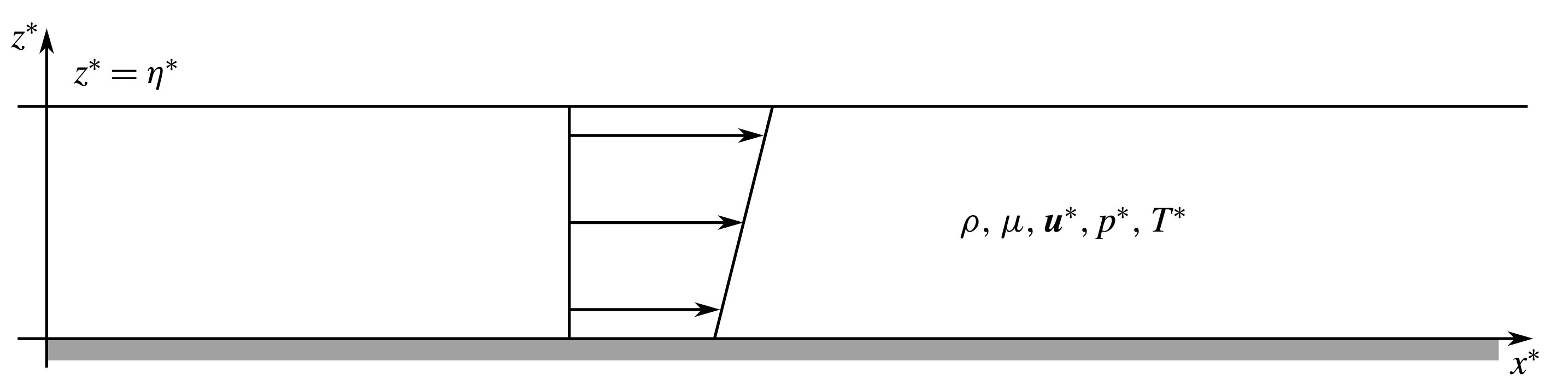
Schematic of the geometry of the problem.
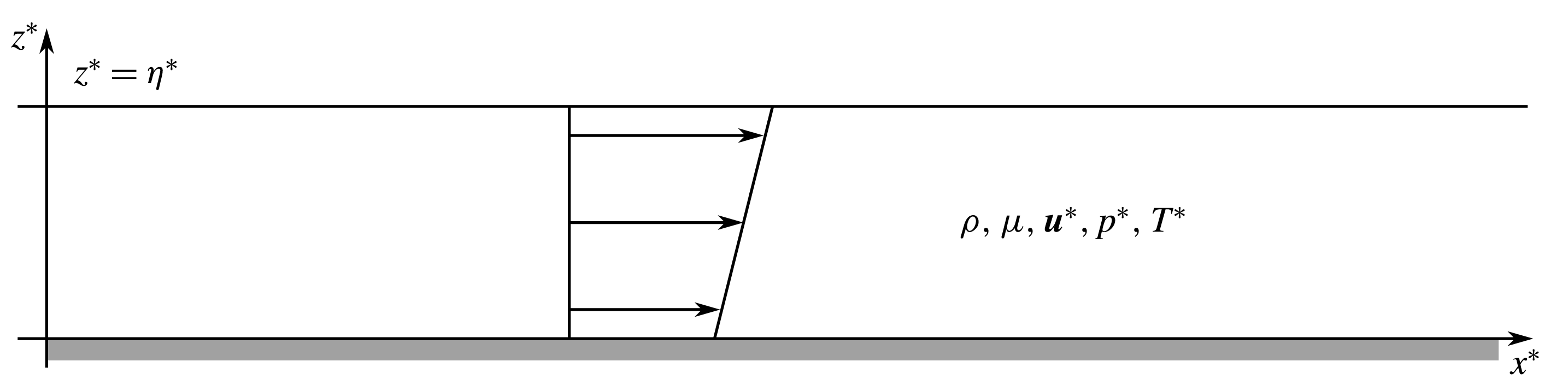
Consider a three-dimensional liquid layer of mean depth
 $d$
under a uniform, horizontal temperature gradient
 $\unicode[STIX]{x2202}T^{\ast }/\unicode[STIX]{x2202}x^{\ast }=-b$
in the coordinate system illustrated in figure 2. The layer is bounded from below by a rigid, partial-slip surface at
 $z^{\ast }=0$
and a free liquid–gas surface from above, at
 $z^{\ast }=\unicode[STIX]{x1D702}^{\ast }$
. The layer consists of an incompressible, Newtonian fluid of viscosity
 $\unicode[STIX]{x1D707}$
, density
 $\unicode[STIX]{x1D70C}$
, velocity
 $\boldsymbol{u}^{\ast }$
and pressure field
 $p^{\ast }$
. Its specific heat, thermal conductivity and thermal surface conductance are denoted by
 $c_{p}$
,
 $k$
and
 $h$
, respectively. Because film thicknesses are of the order of
 $100~\unicode[STIX]{x03BC}\text{m}$
, it is accepted in the literature that gravity in 3DP environments is negligible. The surface tension
 $\unicode[STIX]{x1D70E}_{s}^{\ast }$
of the upper surface decreases as the temperature increases from its reference value,
 $$\begin{eqnarray}\displaystyle \unicode[STIX]{x1D70E}_{s}^{\ast }=\unicode[STIX]{x1D70E}_{0}^{\ast }-\unicode[STIX]{x1D6FE}(T^{\ast }-T_{0}). & & \displaystyle\end{eqnarray}$$
We non-dimensionalize as follows:
 $$\begin{eqnarray}\displaystyle \boldsymbol{x}^{\ast }=d\boldsymbol{x},\quad t^{\ast }=\frac{\unicode[STIX]{x1D707}}{\unicode[STIX]{x1D6FE}b}t,\quad \boldsymbol{u}^{\ast }=\frac{\unicode[STIX]{x1D6FE}bd}{\unicode[STIX]{x1D707}}\boldsymbol{u}=\frac{\unicode[STIX]{x1D6FE}bd}{\unicode[STIX]{x1D707}}(u,v,w), & & \displaystyle\end{eqnarray}$$
 $$\begin{eqnarray}\displaystyle p^{\ast }=\unicode[STIX]{x1D6FE}bp,\quad T^{\ast }-T_{0}=bdT,\quad \unicode[STIX]{x1D70E}_{s}^{\ast }=\unicode[STIX]{x1D70E}_{0}^{\ast }\unicode[STIX]{x1D70E}_{s}. & & \displaystyle\end{eqnarray}$$
In dimensionless terms,
 $$\begin{eqnarray}\displaystyle \unicode[STIX]{x1D70E}_{s}=1-CaT, & & \displaystyle\end{eqnarray}$$
where
 $$\begin{eqnarray}\displaystyle Ca=\frac{\unicode[STIX]{x1D6FE}bd}{\unicode[STIX]{x1D70E}_{0}} & & \displaystyle\end{eqnarray}$$
is the capillary number. Hereafter, the interface is assumed to remain flat,
 $\unicode[STIX]{x1D702}=1$
, which occurs in the limit of zero capillary number, and we assume that the upper layer is a gas of negligible density and zero pressure. The kinematic boundary condition, thermo-capillary stress conditions and heat flux condition at the upper interface become
 $$\begin{eqnarray}\displaystyle & \displaystyle w=0, & \displaystyle\end{eqnarray}$$
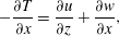 $$\begin{eqnarray}\displaystyle & \displaystyle -\frac{\unicode[STIX]{x2202}T}{\unicode[STIX]{x2202}x}=\frac{\unicode[STIX]{x2202}u}{\unicode[STIX]{x2202}z}+\frac{\unicode[STIX]{x2202}w}{\unicode[STIX]{x2202}x}, & \displaystyle\end{eqnarray}$$
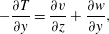 $$\begin{eqnarray}\displaystyle & \displaystyle -\frac{\unicode[STIX]{x2202}T}{\unicode[STIX]{x2202}y}=\frac{\unicode[STIX]{x2202}v}{\unicode[STIX]{x2202}z}+\frac{\unicode[STIX]{x2202}w}{\unicode[STIX]{x2202}y}, & \displaystyle\end{eqnarray}$$
and
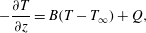 $$\begin{eqnarray}\displaystyle -\frac{\unicode[STIX]{x2202}T}{\unicode[STIX]{x2202}z}=B(T-T_{\infty })+Q, & & \displaystyle\end{eqnarray}$$
at
 $z=1$
, where
 $$\begin{eqnarray}\displaystyle B=\frac{hd}{k} & & \displaystyle\end{eqnarray}$$
is the Biot number,
 $Q$
is a dimensionless surface heat flux determined by the basic state and
 $T_{\infty }$
is the temperature of the bounding gas far from the interface. We impose partial slip and no penetration at the lower boundary
 $$\begin{eqnarray}\displaystyle \frac{\unicode[STIX]{x2202}u}{\unicode[STIX]{x2202}z}=\unicode[STIX]{x1D6FD}u,\quad \frac{\unicode[STIX]{x2202}v}{\unicode[STIX]{x2202}z}=\unicode[STIX]{x1D6FD}v,\quad w=0\quad (z=0), & & \displaystyle\end{eqnarray}$$
as well as the heat flux condition,
 $$\begin{eqnarray}\displaystyle -\boldsymbol{n}\boldsymbol{\cdot }\unicode[STIX]{x1D735}T=B_{l}(T-T_{\infty })\quad (z=0). & & \displaystyle\end{eqnarray}$$
Here,
 $\unicode[STIX]{x1D6FD}$
is a dimensionless slip parameter and
 $B_{l}$
is a lower-boundary Biot number.
Within the layer, the momentum balance is given in dimensionless form by
 $$\begin{eqnarray}\displaystyle R\left[\frac{\unicode[STIX]{x2202}\boldsymbol{u}}{\unicode[STIX]{x2202}t}+\boldsymbol{u}\boldsymbol{\cdot }\unicode[STIX]{x1D735}\boldsymbol{u}\right]=-\unicode[STIX]{x1D735}p+\unicode[STIX]{x1D6FB}^{2}\boldsymbol{u}\quad (0<z<\unicode[STIX]{x1D702}), & & \displaystyle\end{eqnarray}$$
supplemented by the incompressibility condition
 $$\begin{eqnarray}\displaystyle \unicode[STIX]{x1D735}\boldsymbol{\cdot }\boldsymbol{u}=0\quad (0<z<\unicode[STIX]{x1D702}), & & \displaystyle\end{eqnarray}$$
and the heat balance equation
 $$\begin{eqnarray}\displaystyle M\left[\frac{\unicode[STIX]{x2202}T}{\unicode[STIX]{x2202}t}+\boldsymbol{u}\boldsymbol{\cdot }\unicode[STIX]{x1D735}T\right]=\unicode[STIX]{x1D6FB}^{2}T\quad (0<z<\unicode[STIX]{x1D702}), & & \displaystyle\end{eqnarray}$$
where
 $$\begin{eqnarray}\displaystyle R=\frac{\unicode[STIX]{x1D70C}\unicode[STIX]{x1D6FE}bd^{2}}{\unicode[STIX]{x1D707}^{2}}, & & \displaystyle\end{eqnarray}$$
and
 $$\begin{eqnarray}\displaystyle M=\frac{\unicode[STIX]{x1D70C}\unicode[STIX]{x1D6FE}bd^{2}c_{p}}{\unicode[STIX]{x1D707}k}, & & \displaystyle\end{eqnarray}$$
are the Reynolds number and the Marangoni number, respectively. Another useful quantity is the Prandtl number
 $$\begin{eqnarray}\displaystyle Pr=\frac{M}{R}=\frac{\unicode[STIX]{x1D707}c_{p}}{k}. & & \displaystyle\end{eqnarray}$$
2.1 Basic state
We consider the partial-slip shear-flow solution given by
 $$\begin{eqnarray}\displaystyle \bar{u}=-\frac{\unicode[STIX]{x2202}\bar{T}}{\unicode[STIX]{x2202}x}(z+1/\unicode[STIX]{x1D6FD}),\quad \bar{v}=\bar{w}=0,\quad \bar{p}=p_{0}, & & \displaystyle\end{eqnarray}$$
for which the corresponding temperature field,
 $$\begin{eqnarray}\displaystyle \bar{T} & = & \displaystyle -x+M\left[\frac{1}{6}\left(1-z^{3}\right)+\frac{1}{2\unicode[STIX]{x1D6FD}}\left(1-z^{2}\right)+B^{-1}\left(\frac{1}{2}+\frac{1}{\unicode[STIX]{x1D6FD}}\right)+QM^{-1}B^{-1}\right]\nonumber\\ \displaystyle & & \displaystyle -\,B_{l}\unicode[STIX]{x1D6FE}(1+B(1-z)),\end{eqnarray}$$
where
 $$\begin{eqnarray}\displaystyle \unicode[STIX]{x1D6FE}=\frac{M(3(\unicode[STIX]{x1D6FD}+2)+(\unicode[STIX]{x1D6FD}+3)B)-6\unicode[STIX]{x1D6FD}Q}{6\unicode[STIX]{x1D6FD}B(BB_{l}+B+B_{l})}, & & \displaystyle\end{eqnarray}$$
and the temperature of the bounding gas,
 $$\begin{eqnarray}\displaystyle T_{\infty }=-x, & & \displaystyle\end{eqnarray}$$
both have a linear horizontal gradient. This is the unique parallel-flow solution under no imposed pressure gradient. The parameter
 $Q$
is determined by the basic state to ensure continuity of temperature at the upper surface. For
 $\unicode[STIX]{x1D6FD}$
fixed, we fix
 $Q$
so that
 $$\begin{eqnarray}\displaystyle Q=\frac{M(3\unicode[STIX]{x1D6FD}+(2\unicode[STIX]{x1D6FD}+3)B_{l}+6)}{6\unicode[STIX]{x1D6FD}(B_{l}+1)}, & & \displaystyle\end{eqnarray}$$
giving,
 $$\begin{eqnarray}\displaystyle \bar{T}=-x-\frac{M(z-1)(z(z\unicode[STIX]{x1D6FD}+\unicode[STIX]{x1D6FD}+3)(B_{l}+1)+3+\unicode[STIX]{x1D6FD})}{6\unicode[STIX]{x1D6FD}(B_{l}+1)}. & & \displaystyle\end{eqnarray}$$
When
 $\unicode[STIX]{x1D6FD}\rightarrow \infty$
and
 $B_{l}=0$
,
 $$\begin{eqnarray}\displaystyle \bar{u}\rightarrow -z\frac{\unicode[STIX]{x2202}\bar{T}}{\unicode[STIX]{x2202}x},\quad \bar{v}=\bar{w}=0,\quad \bar{p}=p_{0}, & & \displaystyle\end{eqnarray}$$
 $$\begin{eqnarray}\displaystyle \bar{T}\rightarrow -x+M\left[{\textstyle \frac{1}{6}}(1-z^{3})\right], & & \displaystyle\end{eqnarray}$$
which recovers the no-slip limit of Smith & Davis (Reference Smith and Davis1983a ).
2.2 Linear stability analysis
Introduce perturbations
 $X=\bar{X}+\unicode[STIX]{x1D716}X^{\prime }$
, where
 $X=(\boldsymbol{u},p,T)$
. The perturbations are governed by
 $$\begin{eqnarray}\displaystyle & \displaystyle R\left[\frac{\unicode[STIX]{x2202}\boldsymbol{u}}{\unicode[STIX]{x2202}t}+\bar{u}\frac{\unicode[STIX]{x2202}\boldsymbol{u}^{\prime }}{\unicode[STIX]{x2202}x}+w^{\prime }\frac{\unicode[STIX]{x2202}\bar{u}}{\unicode[STIX]{x2202}z}\boldsymbol{e}_{\boldsymbol{x}}\right]=-\unicode[STIX]{x1D735}p^{\prime }+\unicode[STIX]{x1D6FB}^{2}\boldsymbol{u}^{\prime }, & \displaystyle\end{eqnarray}$$
 $$\begin{eqnarray}\displaystyle & \displaystyle M\left[\frac{\unicode[STIX]{x2202}T^{\prime }}{\unicode[STIX]{x2202}t}+\bar{u}\frac{\unicode[STIX]{x2202}T^{\prime }}{\unicode[STIX]{x2202}x}+u^{\prime }\frac{\unicode[STIX]{x2202}\bar{T}}{\unicode[STIX]{x2202}x}+w^{\prime }\frac{\unicode[STIX]{x2202}\bar{T}}{\unicode[STIX]{x2202}z}\right]=\unicode[STIX]{x1D6FB}^{2}T^{\prime }, & \displaystyle\end{eqnarray}$$
 $$\begin{eqnarray}\displaystyle & \displaystyle \unicode[STIX]{x1D735}\boldsymbol{\cdot }\boldsymbol{u}^{\prime }=0, & \displaystyle\end{eqnarray}$$
and are subject to the boundary conditions
 $$\begin{eqnarray}\displaystyle & \displaystyle w^{\prime }=0\quad (z=1), & \displaystyle\end{eqnarray}$$
 $$\begin{eqnarray}\displaystyle & \displaystyle \frac{\unicode[STIX]{x2202}u^{\prime }}{\unicode[STIX]{x2202}z}+\frac{\unicode[STIX]{x2202}w^{\prime }}{\unicode[STIX]{x2202}x}=-\frac{\unicode[STIX]{x2202}T^{\prime }}{\unicode[STIX]{x2202}x}\quad (z=1), & \displaystyle\end{eqnarray}$$
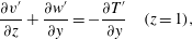 $$\begin{eqnarray}\displaystyle & \displaystyle \frac{\unicode[STIX]{x2202}v^{\prime }}{\unicode[STIX]{x2202}z}+\frac{\unicode[STIX]{x2202}w^{\prime }}{\unicode[STIX]{x2202}y}=-\frac{\unicode[STIX]{x2202}T^{\prime }}{\unicode[STIX]{x2202}y}\quad (z=1), & \displaystyle\end{eqnarray}$$
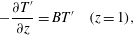 $$\begin{eqnarray}\displaystyle & \displaystyle -\frac{\unicode[STIX]{x2202}T^{\prime }}{\unicode[STIX]{x2202}z}=BT^{\prime }\quad (z=1), & \displaystyle\end{eqnarray}$$
 $$\begin{eqnarray}\displaystyle \frac{\unicode[STIX]{x2202}u^{\prime }}{\unicode[STIX]{x2202}z}=\unicode[STIX]{x1D6FD}u^{\prime },\quad \frac{\unicode[STIX]{x2202}v^{\prime }}{\unicode[STIX]{x2202}z}=\unicode[STIX]{x1D6FD}v^{\prime },\quad w^{\prime }=0,\quad \frac{\unicode[STIX]{x2202}T^{\prime }}{\unicode[STIX]{x2202}z}=B_{l}T^{\prime }\quad (z=0). & & \displaystyle\end{eqnarray}$$
We search for normal mode solutions
 $$\begin{eqnarray}\displaystyle (\boldsymbol{u}^{\prime },p^{\prime },T^{\prime })=(\hat{u} (z),\hat{p}(z),\hat{T}(z))\text{e}^{\unicode[STIX]{x1D70E}t+\text{i}\unicode[STIX]{x1D736}\boldsymbol{\cdot }\boldsymbol{x}}, & & \displaystyle\end{eqnarray}$$
where
 $\unicode[STIX]{x1D736}=(\unicode[STIX]{x1D6FC}_{1},\unicode[STIX]{x1D6FC}_{2},0)$
, and obtain a system of differential equations
 $$\begin{eqnarray}\displaystyle & \displaystyle R[\unicode[STIX]{x1D70E}\hat{\boldsymbol{u}}+\text{i}\unicode[STIX]{x1D6FC}_{1}\bar{u}\hat{\boldsymbol{u}}+{\hat{w}}(D\bar{u})\boldsymbol{e}_{\boldsymbol{x}}]=-\text{i}\unicode[STIX]{x1D736}\hat{p}-(D\hat{p})\boldsymbol{e}_{\boldsymbol{z}}+(D^{2}-\unicode[STIX]{x1D6FC}^{2})\hat{\boldsymbol{u}}, & \displaystyle\end{eqnarray}$$
 $$\begin{eqnarray}\displaystyle & \displaystyle M[\unicode[STIX]{x1D70E}\hat{T}+\text{i}\unicode[STIX]{x1D6FC}_{1}\bar{u}\hat{T}-\hat{u} +{\hat{w}}(D\bar{T})]=(D^{2}-\unicode[STIX]{x1D6FC}^{2})\hat{T}, & \displaystyle\end{eqnarray}$$
 $$\begin{eqnarray}\displaystyle & \displaystyle \text{i}\unicode[STIX]{x1D6FC}_{1}\hat{u} +\text{i}\unicode[STIX]{x1D6FC}_{2}\hat{v}+D{\hat{w}}=0, & \displaystyle\end{eqnarray}$$
subject to the boundary conditions
 $$\begin{eqnarray}\displaystyle & \displaystyle {\hat{w}}=0\quad (z=1), & \displaystyle\end{eqnarray}$$
 $$\begin{eqnarray}\displaystyle & \displaystyle D\hat{u} +\text{i}\unicode[STIX]{x1D6FC}_{1}{\hat{w}}=-\text{i}\unicode[STIX]{x1D6FC}_{1}\hat{T}\quad (z=1), & \displaystyle\end{eqnarray}$$
 $$\begin{eqnarray}\displaystyle & \displaystyle D\hat{v}+\text{i}\unicode[STIX]{x1D6FC}_{2}{\hat{w}}=-\text{i}\unicode[STIX]{x1D6FC}_{2}\hat{T}\quad (z=1), & \displaystyle\end{eqnarray}$$
 $$\begin{eqnarray}\displaystyle & \displaystyle -D\hat{T}=B\hat{T}\quad (z=1), & \displaystyle\end{eqnarray}$$
 $$\begin{eqnarray}\displaystyle D\hat{u} =\unicode[STIX]{x1D6FD}\hat{u} ,\quad D\hat{v}=\unicode[STIX]{x1D6FD}\hat{v},\quad {\hat{w}}=0,\quad D\hat{T}=B_{l}\hat{T}\quad (z=0), & & \displaystyle\end{eqnarray}$$
where
 $D=\text{d}/\text{d}z$
is a differential operator and
 $\unicode[STIX]{x1D6FC}=|\unicode[STIX]{x1D736}|$
.
Eliminating
 $\hat{p}$
and
 $\hat{v}$
gives the reduced system
 $$\begin{eqnarray}\displaystyle [(\unicode[STIX]{x1D6FC}^{2}Pr+M(\unicode[STIX]{x1D70E}+\text{i}\unicode[STIX]{x1D6FC}_{1}(z+\unicode[STIX]{x1D6FD}^{-1})))-PrD^{2}](\unicode[STIX]{x1D6FC}^{2}\hat{u} -\text{i}\unicode[STIX]{x1D6FC}_{1}D{\hat{w}})+\unicode[STIX]{x1D6FC}_{2}^{2}M{\hat{w}}=0, & & \displaystyle\end{eqnarray}$$
 $$\begin{eqnarray}\displaystyle & & \displaystyle (\unicode[STIX]{x1D6FC}^{2}Pr+M(\unicode[STIX]{x1D70E}+\text{i}\unicode[STIX]{x1D6FC}_{1}(z+\unicode[STIX]{x1D6FD}^{-1})))(D^{2}{\hat{w}}+\text{i}\unicode[STIX]{x1D6FC}_{1}D\hat{u} -\unicode[STIX]{x1D6FC}_{2}^{2}{\hat{w}})\nonumber\\ \displaystyle & & \displaystyle \quad +\,\unicode[STIX]{x1D6FC}_{2}^{2}PrD^{2}{\hat{w}}-(\unicode[STIX]{x1D6FC}_{1}M+\text{i}PrD^{3})(\unicode[STIX]{x1D6FC}_{1}\hat{u} -\text{i}D{\hat{w}})=0,\end{eqnarray}$$
 $$\begin{eqnarray}\displaystyle (\unicode[STIX]{x1D6FC}^{2}+M(\unicode[STIX]{x1D70E}+\text{i}\unicode[STIX]{x1D6FC}_{1}(z+\unicode[STIX]{x1D6FD}^{-1})))\hat{T}=D^{2}\hat{T}+{\textstyle \frac{1}{2}}M^{2}z(z+2\unicode[STIX]{x1D6FD}^{-1}){\hat{w}}+M\hat{u} , & & \displaystyle\end{eqnarray}$$
subject to
 $$\begin{eqnarray}\displaystyle {\hat{w}} & = & \displaystyle 0\quad (z=1),\end{eqnarray}$$
 $$\begin{eqnarray}\displaystyle \hat{u} ^{\prime }+\text{i}\unicode[STIX]{x1D6FC}_{1}{\hat{w}} & = & \displaystyle -\text{i}\unicode[STIX]{x1D6FC}_{1}\hat{T}\quad (z=1),\end{eqnarray}$$
 $$\begin{eqnarray}\displaystyle -\unicode[STIX]{x1D6FC}_{1}\hat{u} ^{\prime }+\text{i}{\hat{w}}^{\prime \prime }+\text{i}\unicode[STIX]{x1D6FC}_{2}^{2}{\hat{w}} & = & \displaystyle -\text{i}\unicode[STIX]{x1D6FC}_{2}^{2}\hat{T}\quad (z=1),\end{eqnarray}$$
 $$\begin{eqnarray}\displaystyle -\hat{T}^{\prime } & = & \displaystyle B\hat{T}\quad (z=1),\end{eqnarray}$$
 $$\begin{eqnarray}\displaystyle \hat{u} ^{\prime } & = & \displaystyle \unicode[STIX]{x1D6FD}\hat{u} \quad (z=0),\end{eqnarray}$$
 $$\begin{eqnarray}\displaystyle \text{i}{\hat{w}}^{\prime \prime }-\unicode[STIX]{x1D6FC}_{1}\hat{u} ^{\prime } & = & \displaystyle \unicode[STIX]{x1D6FD}(\text{i}{\hat{w}}^{\prime }-\unicode[STIX]{x1D6FC}_{1}\hat{u} )\quad (z=0),\end{eqnarray}$$
 $$\begin{eqnarray}\displaystyle {\hat{w}} & = & \displaystyle 0\quad (z=0),\end{eqnarray}$$
 $$\begin{eqnarray}\displaystyle \hat{T}^{\prime } & = & \displaystyle B_{l}\hat{T}\quad (z=0).\end{eqnarray}$$
2.3 Minimization procedure
The system of differential equations above forms an eight-order eigenvalue problem, which we solve numerically to find allowable values of the growth rate
 $\unicode[STIX]{x1D70E}$
. We are interested in neutral stability and set
 $\text{Re}(\unicode[STIX]{x1D70E})=0$
, so that
 $\unicode[STIX]{x1D70E}=\text{i}\unicode[STIX]{x1D714}$
in terms of the frequency
 $\unicode[STIX]{x1D714}\in \mathbb{R}$
. To obtain non-zero solutions numerically, we note that solutions are defined only up to a multiplicative constant and impose the constraint
 $\hat{T}=1$
at
 $z=1$
, without loss of generality. From this numerical calculation, we obtain the Marangoni number
 $M$
corresponding to the point of neutral stability. This defines a neutral surface, given by
 $$\begin{eqnarray}\displaystyle M=M(\unicode[STIX]{x1D6FC}_{1},\unicode[STIX]{x1D6FC}_{2},Pr,B,B_{l},\unicode[STIX]{x1D6FD}), & & \displaystyle\end{eqnarray}$$
which is supplemented by the corresponding frequency
 $$\begin{eqnarray}\displaystyle \unicode[STIX]{x1D714}=\unicode[STIX]{x1D714}(\unicode[STIX]{x1D6FC}_{1},\unicode[STIX]{x1D6FC}_{2},Pr,B,B_{l},\unicode[STIX]{x1D6FD}). & & \displaystyle\end{eqnarray}$$
The global minimum of the neutral surface defines the critical Marangoni number
 $M_{c}$
, which needs to be exceeded in order for any instabilities to occur. We find the critical Marangoni number by first using Newton’s method to find a local minimum,
 $$\begin{eqnarray}\displaystyle M=M_{m}(j;Pr,B,B_{l},\unicode[STIX]{x1D6FD}), & & \displaystyle\end{eqnarray}$$
of the neutral surface. As there is more than one local minimum, we use
 $j$
as an index to distinguish the various minima, or branches. The corresponding wavevector and frequency are denoted by
 $$\begin{eqnarray}\displaystyle \unicode[STIX]{x1D736} & = & \displaystyle \unicode[STIX]{x1D736}_{m}(j;Pr,B,B_{l},\unicode[STIX]{x1D6FD}),\end{eqnarray}$$
 $$\begin{eqnarray}\displaystyle \unicode[STIX]{x1D714} & = & \displaystyle \unicode[STIX]{x1D714}_{m}(j;Pr,B,B_{l},\unicode[STIX]{x1D6FD}).\end{eqnarray}$$
By changing the initial guess in the minimization process, we obtain all local minima,
 $M_{m}$
, of the neutral surface. There is a finite number of local minima. The smallest value of
 $M_{m}$
defines the critical Marangoni number
 $$\begin{eqnarray}\displaystyle M=M_{c}(Pr,B,B_{l},\unicode[STIX]{x1D6FD}), & & \displaystyle\end{eqnarray}$$
and the corresponding critical wavevector and frequency
 $$\begin{eqnarray}\displaystyle \unicode[STIX]{x1D736} & = & \displaystyle \unicode[STIX]{x1D736}_{c}(Pr,B,B_{l},\unicode[STIX]{x1D6FD}),\end{eqnarray}$$
 $$\begin{eqnarray}\displaystyle \unicode[STIX]{x1D714} & = & \displaystyle \unicode[STIX]{x1D714}_{c}(Pr,B,B_{l},\unicode[STIX]{x1D6FD}).\end{eqnarray}$$
We repeat this procedure for a range of values of
 $Pr,B,B_{l}$
and
 $\unicode[STIX]{x1D6FD}$
belonging to the interval
 $[0,\infty )$
via parameter continuation.
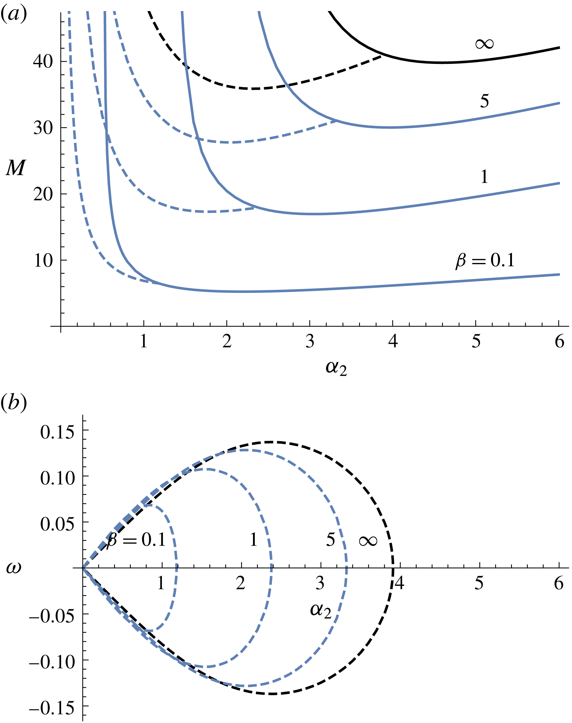
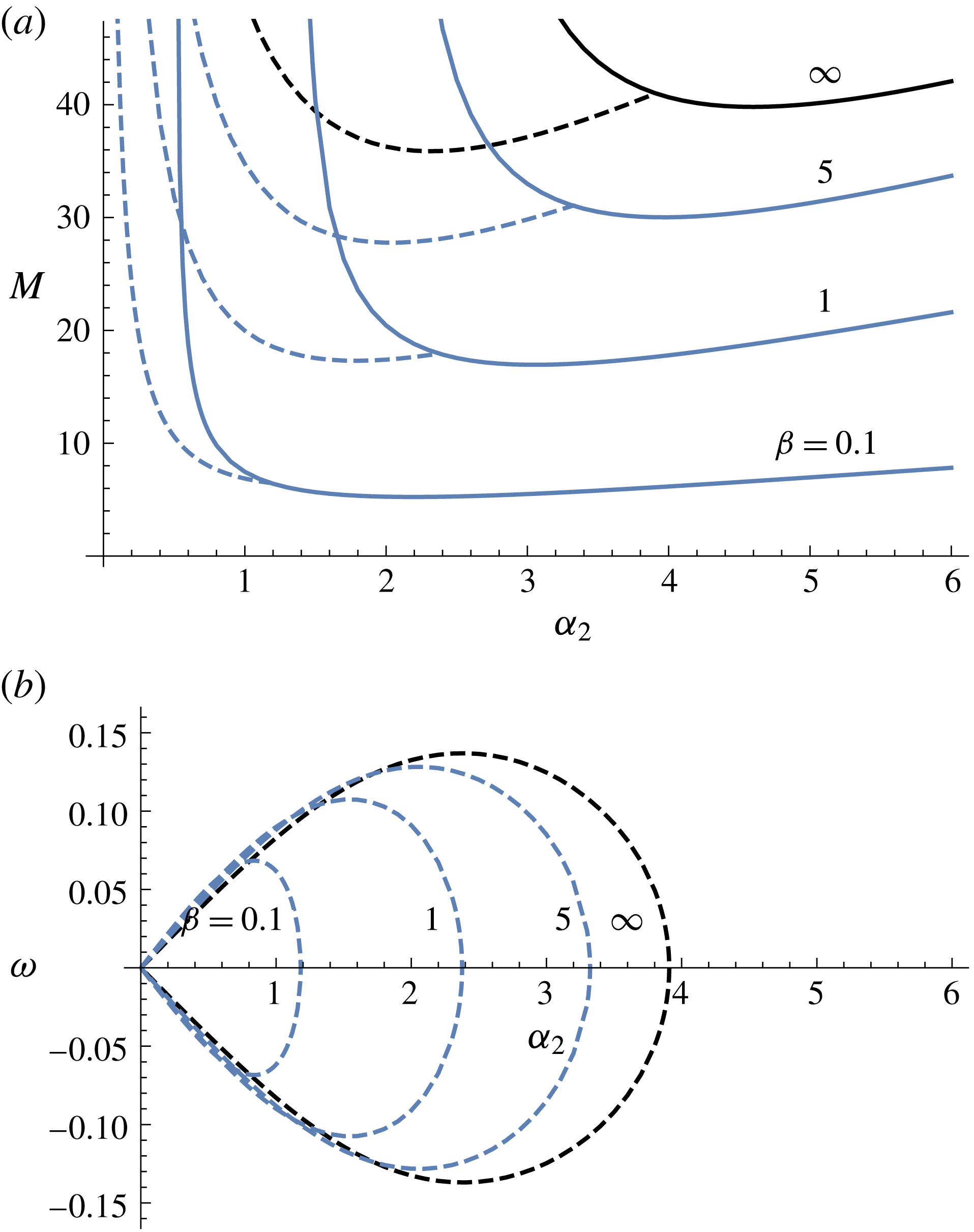
Neutral curves, depicting (
 $a$
)
 $M$
and (
 $b$
)
 $\unicode[STIX]{x1D714}$
for various slip parameters and
 $Pr=1/2$
,
 $B=5$
,
 $B_{l}=0$
. The solid curves depict longitudinal rolls, and the dashed curves depict longitudinal travelling waves.
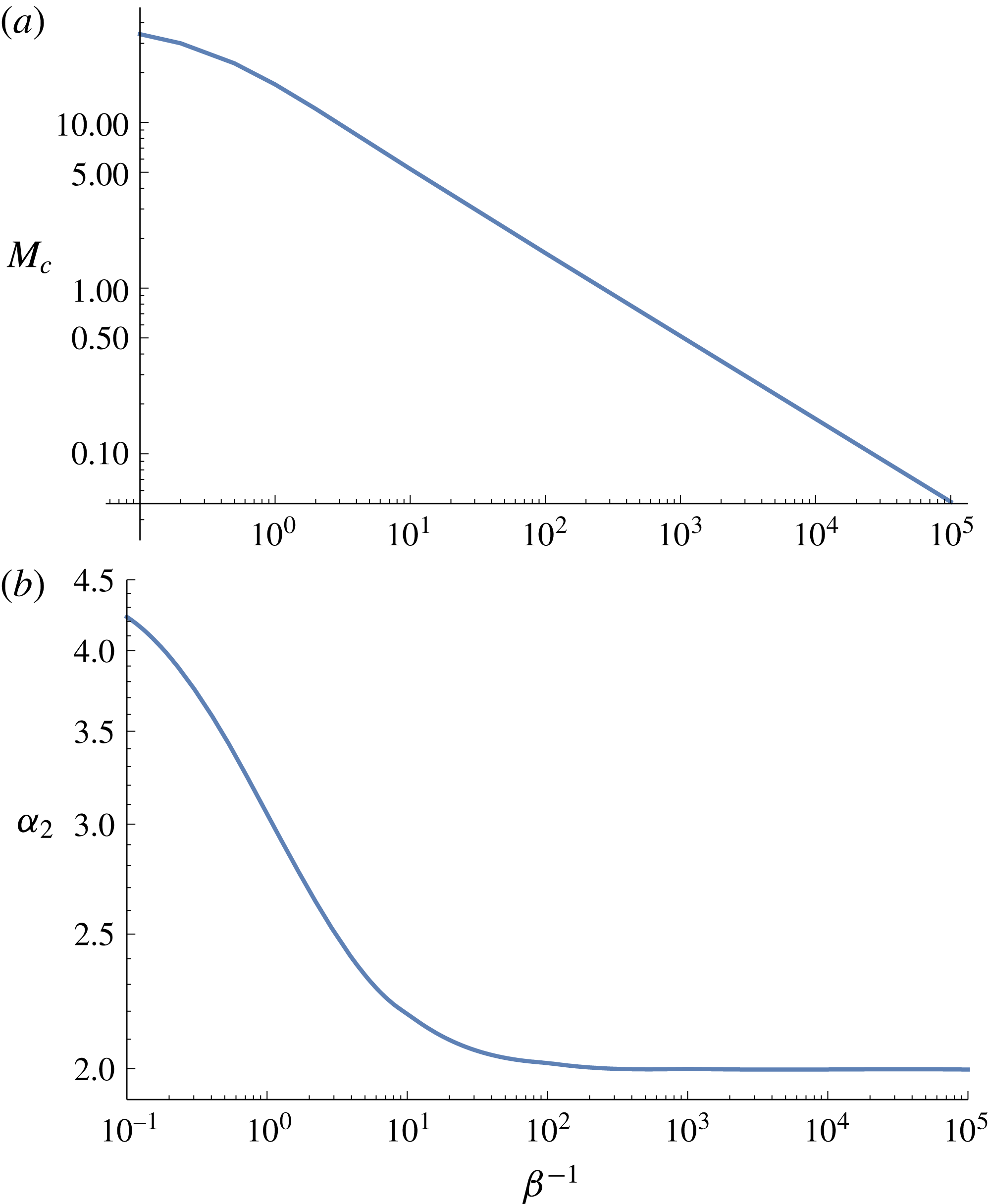
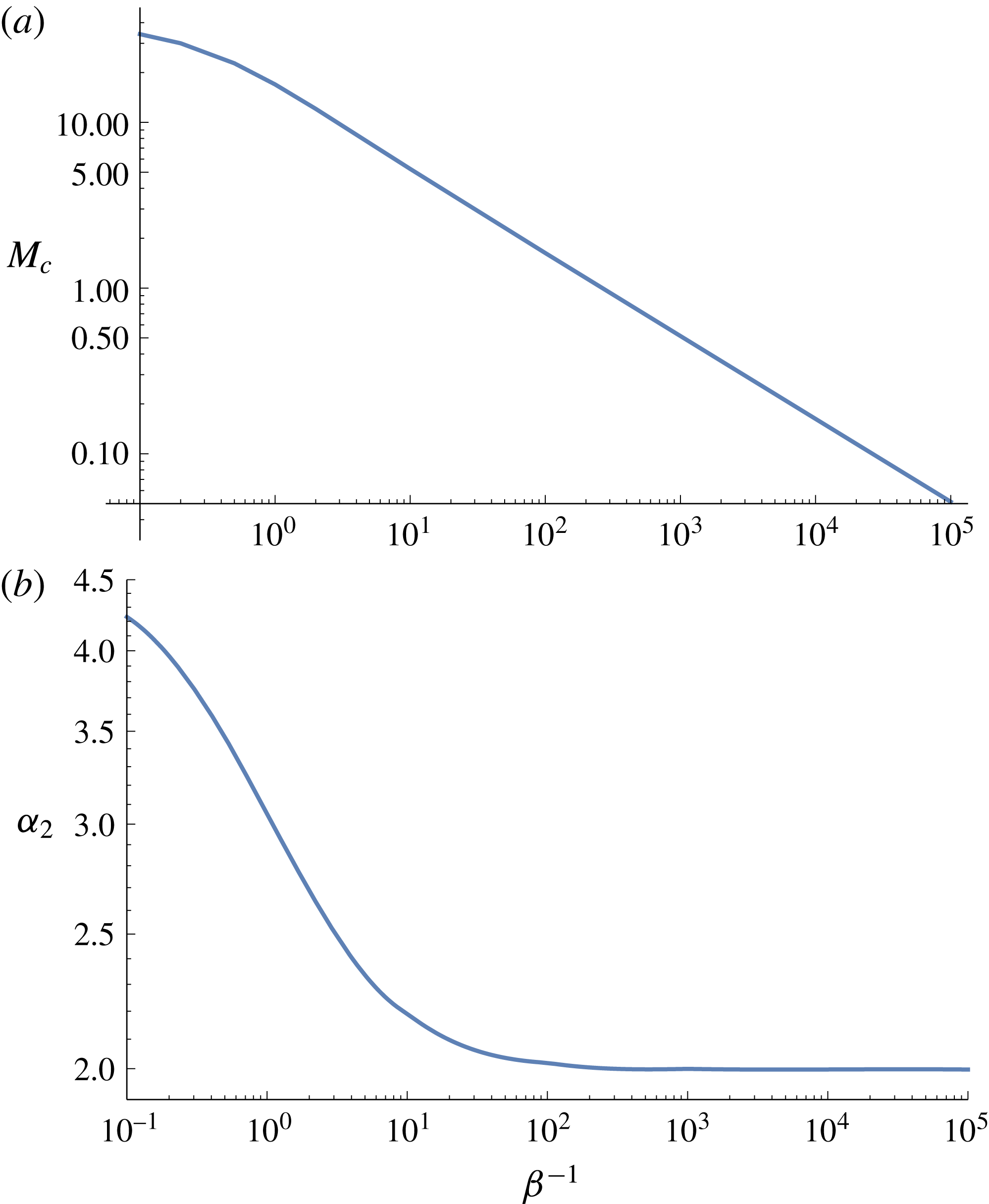
Critical (
 $a$
) Marangoni number and (
 $b$
) wavenumber for longitudinal rolls against
 $\unicode[STIX]{x1D6FD}^{-1}$
. The wavenumber tends to an asymptotic value of approximately 2 as
 $\unicode[STIX]{x1D6FD}^{-1}\rightarrow \infty$
. Parameters:
 $B=5,B_{l}=0,Pr=1/2$
.
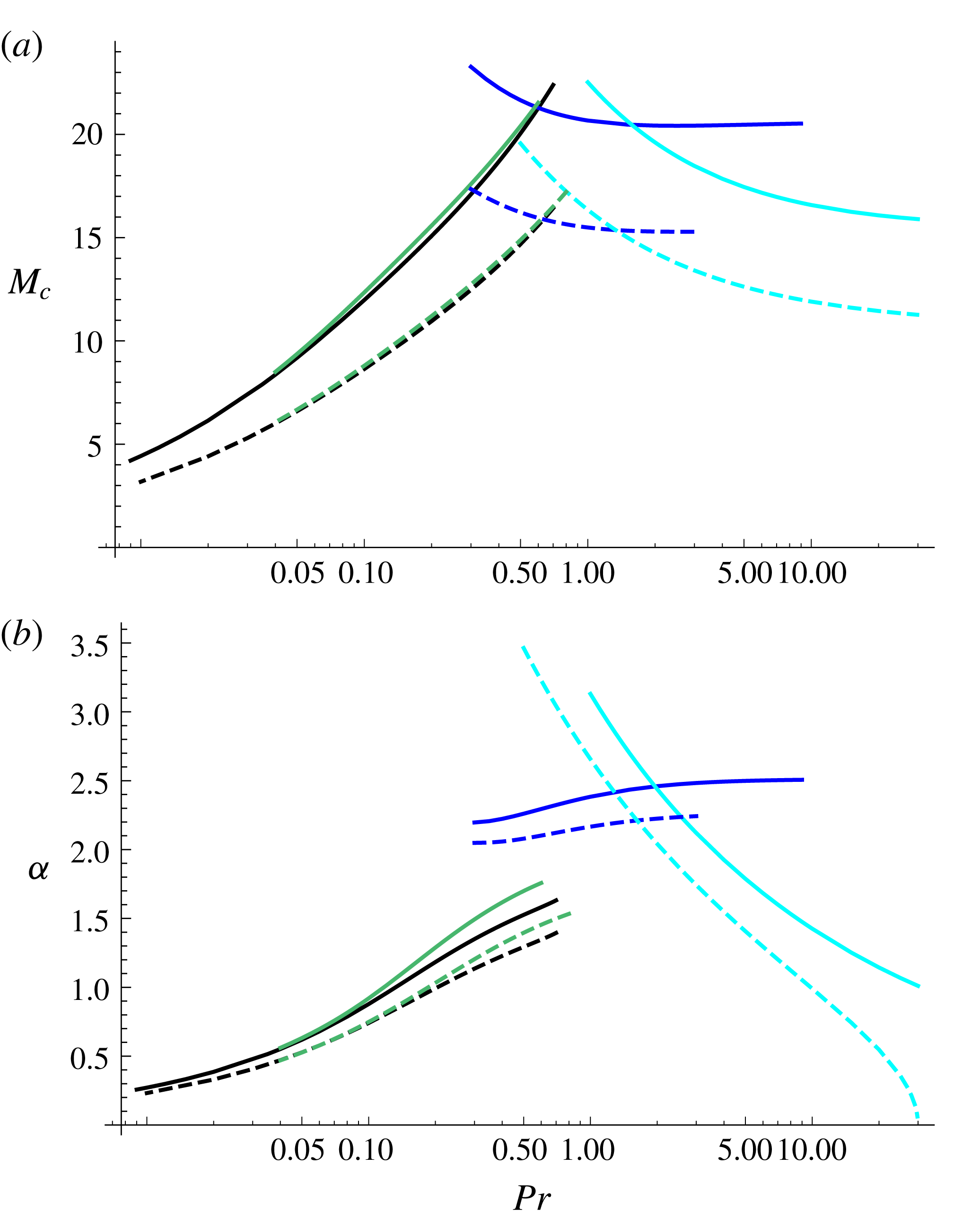
Critical values of (
 $a$
)
 $M$
and (
 $b$
)
 $\unicode[STIX]{x1D6FC}$
for
 $B=B_{l}=0$
, in the no-slip limit (solid curves) and partial slip with
 $\unicode[STIX]{x1D6FD}=5$
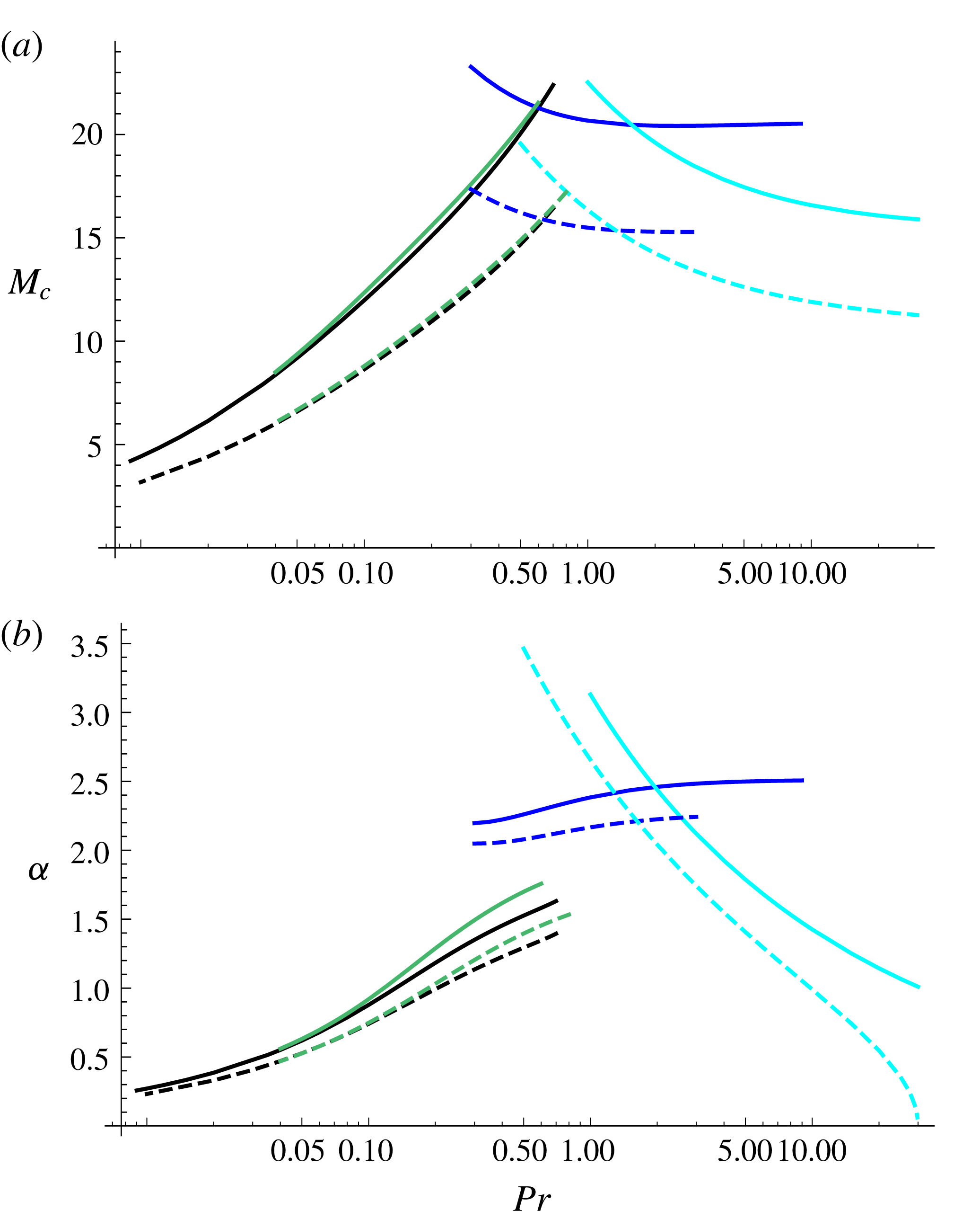
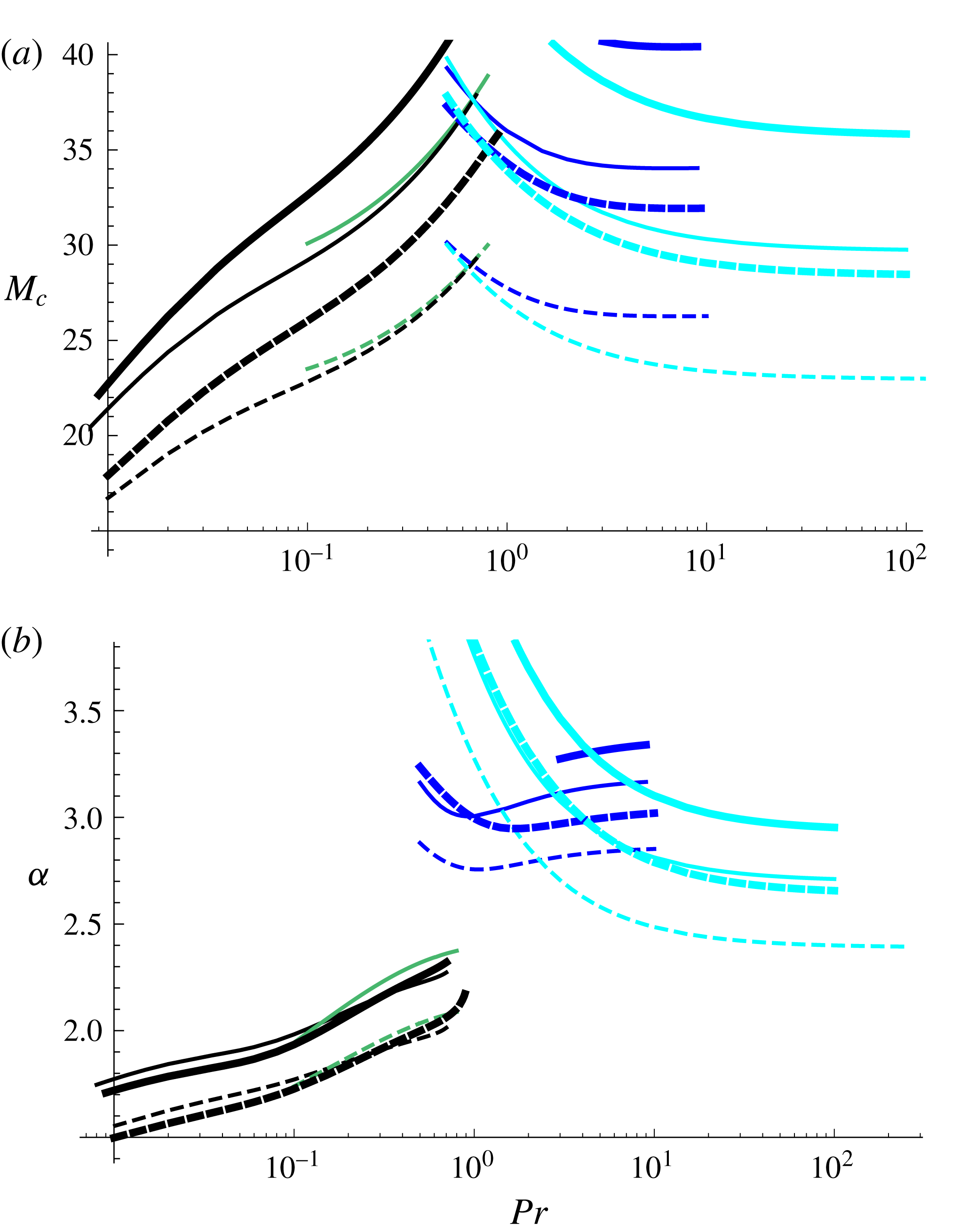
(dashed curves) for oblique hydrothermal waves (black), two-dimensional hydrothermal waves (blue), longitudinal rolls (cyan) and longitudinal waves (green). The preferred mode is given by the lowest value of
 $M$
for each
 $Pr$
. Slip destabilizes the system for all types of modes.
Critical values of (
 $a$
)
 $M$
and (
 $b$
)
 $\unicode[STIX]{x1D6FC}$
for
 $B=5$
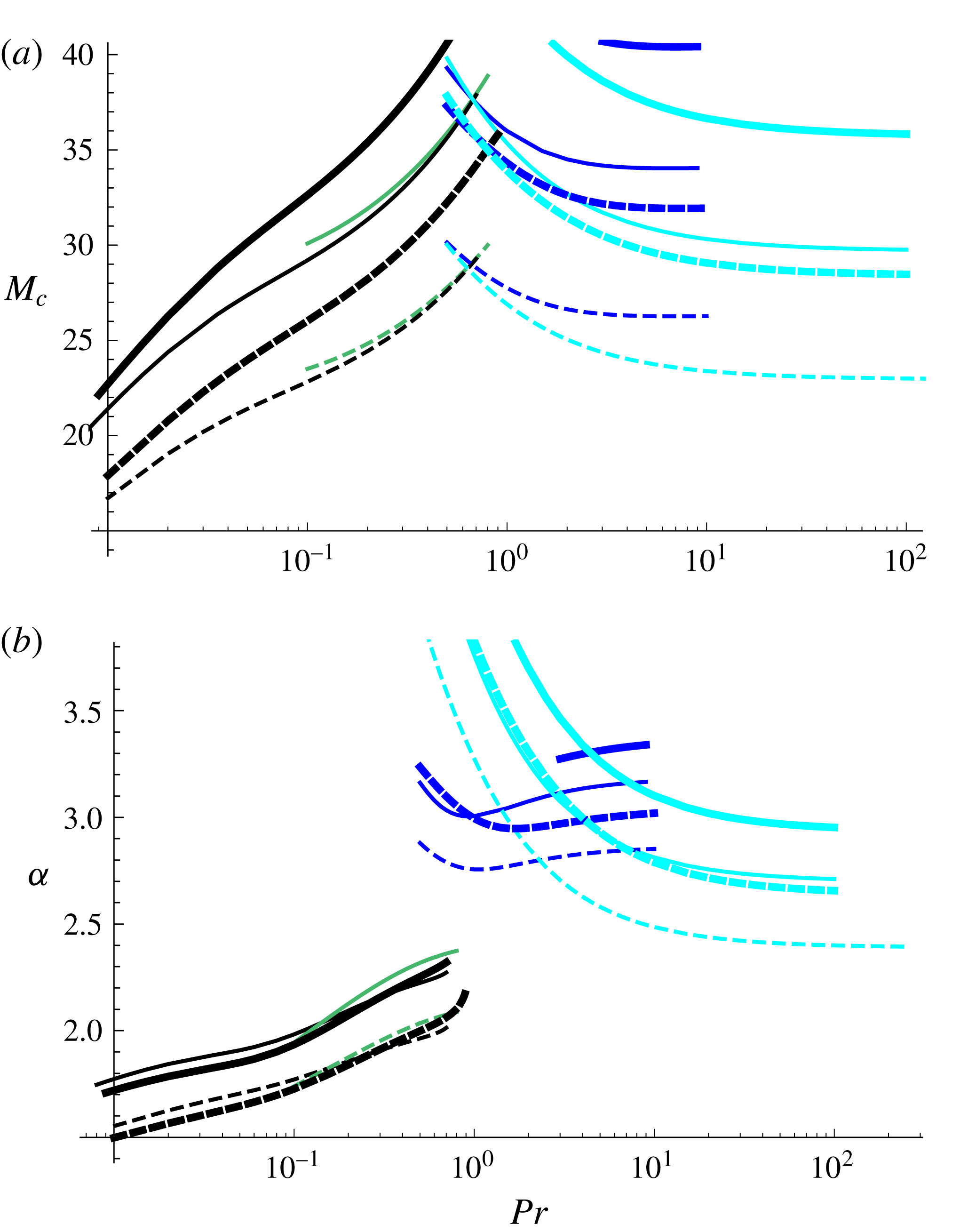
, in the no-slip limit (solid curves) and partial slip with
 $\unicode[STIX]{x1D6FD}=5$
(dashed curves) for oblique hydrothermal waves (black), two-dimensional hydrothermal waves (blue), longitudinal rolls (cyan) and longitudinal waves (green). Thin curves correspond to
 $B_{l}=0$
. Thick curves correspond to
 $B_{l}=1$
. The preferred mode is given by the lowest value of
 $M$
for each
 $Pr$
.
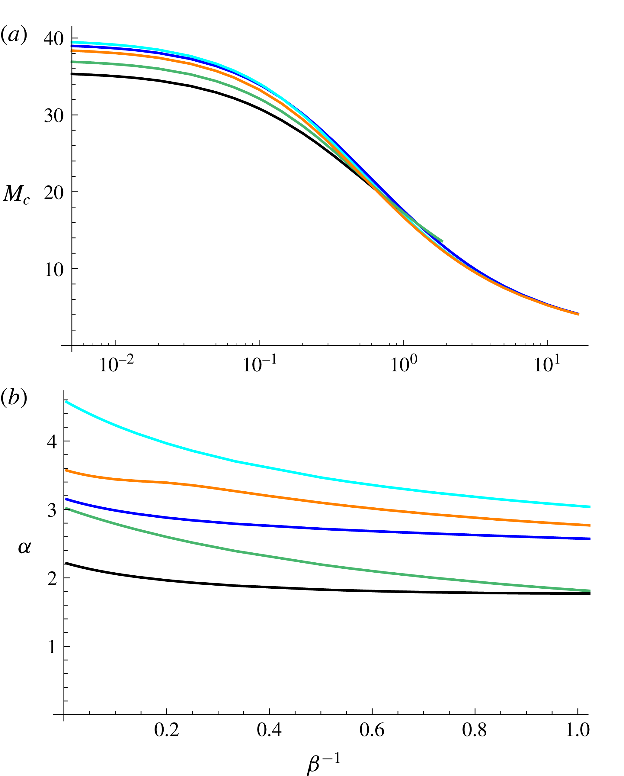
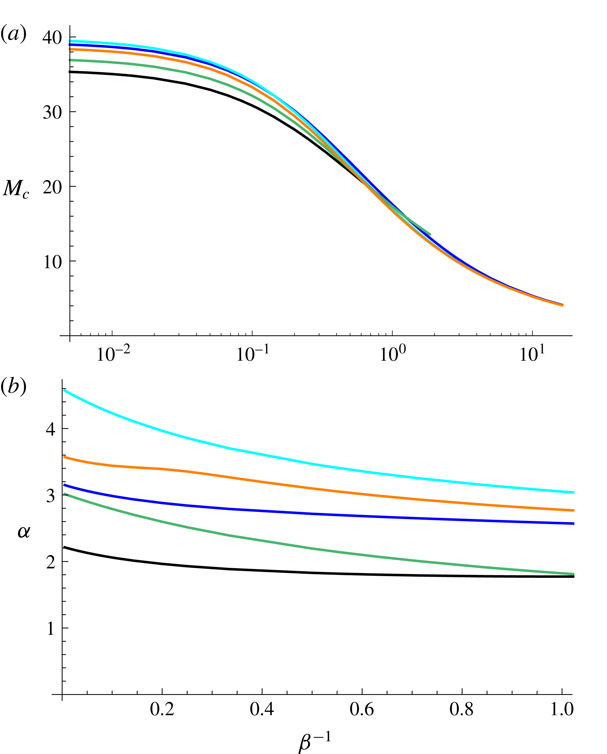
Minimal (
 $a$
) Marangoni number and (
 $b$
) associated wavenumber for
 $Pr=1/2$
,
 $B=5$
and
 $B_{l}=0$
. Longitudinal rolls are shown in cyan
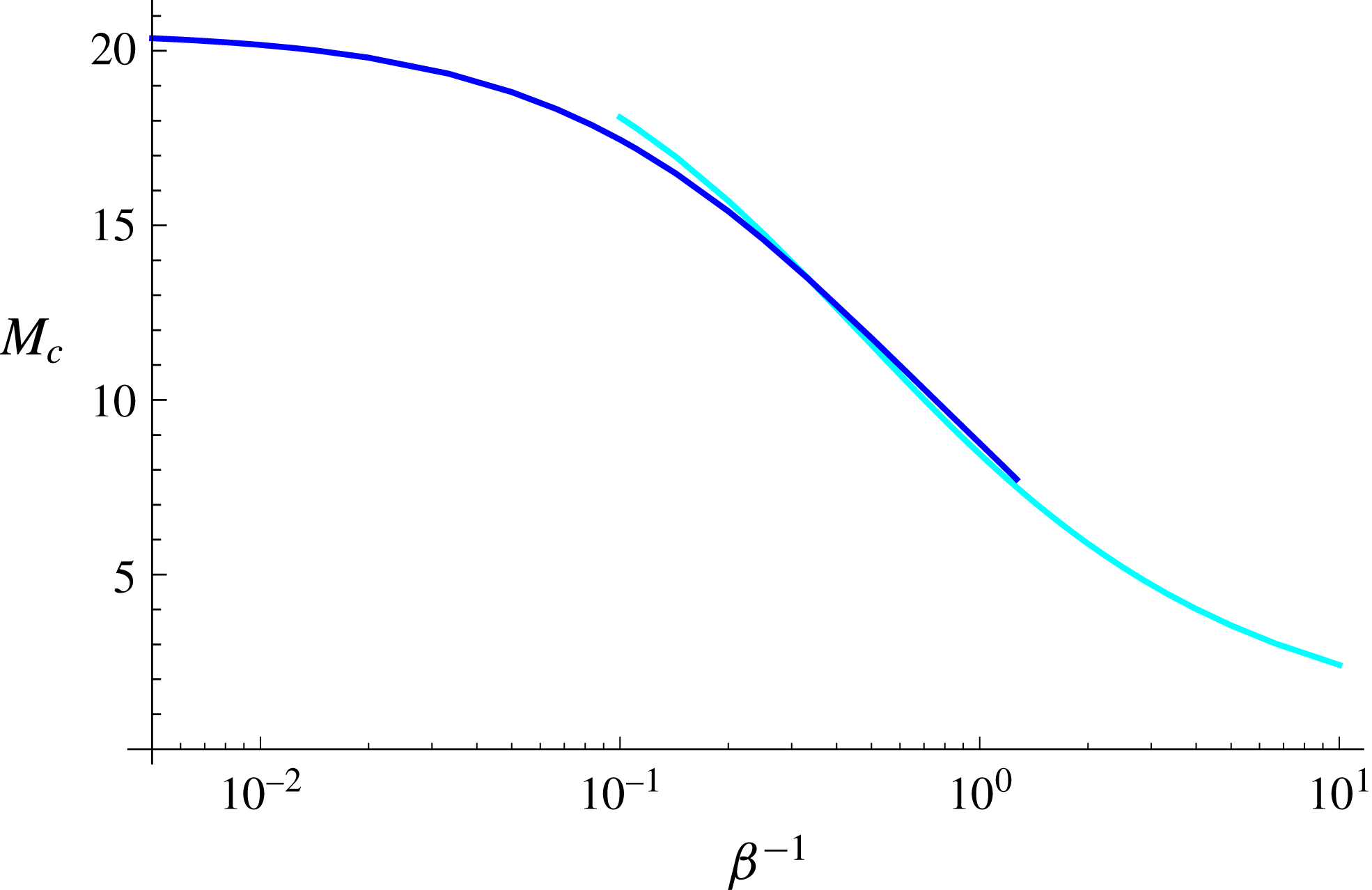
 $(M_{m}\sim 20.2(\unicode[STIX]{x1D6FD}^{-1}+0.33)^{-0.61})$
, longitudinal waves are shown in green
 $(M_{m}\sim 19.8(\unicode[STIX]{x1D6FD}^{-1}+0.29)^{-0.51})$
, oblique hydrothermal waves are shown in black
 $(M_{m}\sim 19.6(\unicode[STIX]{x1D6FD}^{-1}+0.29)^{-0.48})$
and orange
 $(M_{m}\sim 19.4(\unicode[STIX]{x1D6FD}^{-1}+0.29)^{-0.56})$
and two-dimensional hydrothermal waves are shown in blue
 $(M_{m}\sim 21.1(\unicode[STIX]{x1D6FD}^{-1}+0.35)^{-0.60})$
.
3 Longitudinal instabilities
We first confine attention to the case in which
 $\unicode[STIX]{x1D6FC}_{1}=0$
, giving rise to longitudinal instabilities. Two types of longitudinal instabilities appear: longitudinal rolls and longitudinal travelling waves.
3.1 Stationary longitudinal rolls
The onset of stationary longitudinal rolls occurs with
 $\unicode[STIX]{x1D714}=0$
and axes aligned in the direction of the mean flow. Neutral curves for various slip parameters at fixed
 $Pr$
are depicted in figure 3. The minimum of each neutral curve defines the minimal Marangoni number
 $M_{m}$
necessary for the onset of instability, which corresponds to an associated transverse wavenumber
 $\unicode[STIX]{x1D6FC}_{2m}$
. Each of these decreases as the slip parameter
 $\unicode[STIX]{x1D6FD}^{-1}$
increases. Basal slip destabilizes the system. The neutral curve in the no-slip limit is an upper bound, towards which the remaining neutral curves tend to monotonically as
 $\unicode[STIX]{x1D6FD}\rightarrow \infty$
.
The minimal Marangoni number for the onset of stationary longitudinal rolls decreases monotonically from
 $M_{m}\approx 40$
in the no-slip limit towards zero as
 $\unicode[STIX]{x1D6FD}^{-1}\rightarrow \infty$
as depicted in figure 4(a). The associated wavenumber approaches a non-zero value in the limit
 $\unicode[STIX]{x1D6FD}^{-1}\rightarrow \infty$
as depicted in figure 4(b).
These minima do not necessarily reflect the preferred modes of instability, as the preferred mode need not be longitudinal. This is the case for low and moderate Prandtl numbers, as seen in figure 5(a). The preferred mode is given by the lowest value of
 $M$
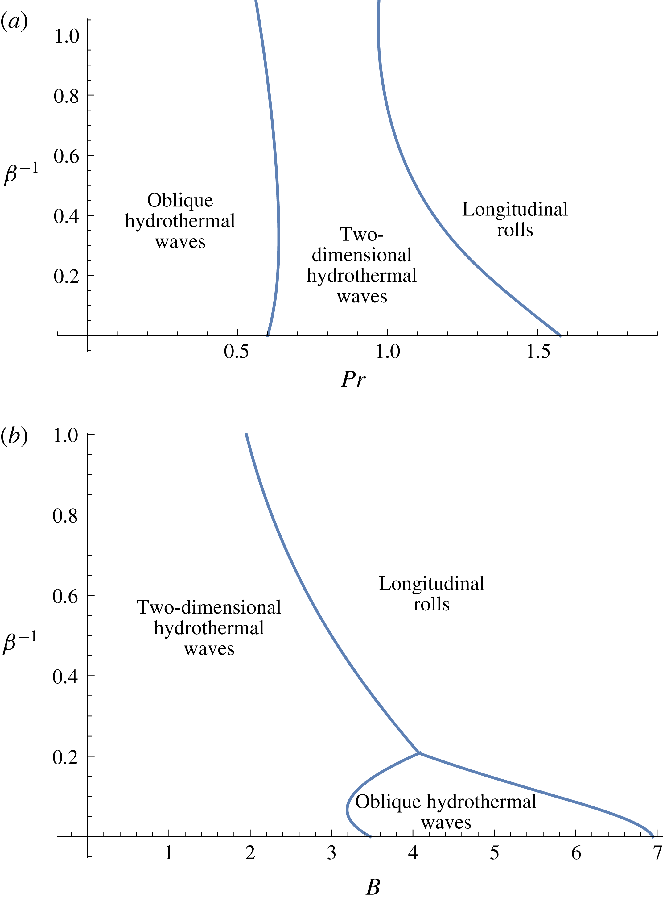
for each Prandtl number. By the preferred mode, we refer to the mode that is seen most visibly in experiment or practical application. For large enough Prandtl numbers, however, stationary longitudinal rolls are the preferred modes of instability as seen in figures 14(a) and 5(a), both with and without slip, for
 $B=0$
. Longitudinal rolls can also be preferred for lower Prandtl numbers, as long as the Biot number is large enough, as seen in figure 14(b).
Slip is seen to destabilize the system. Both with and without slip, the magnitude of the critical wavenumber for stationary longitudinal rolls decreases monotonically with the Prandtl number as seen in figure 5(b). However, the system selects long wave instabilities near a critical, finite Prandtl number,
 $Pr\approx 30$
, for
 $B=B_{l}=0$
,
 $\unicode[STIX]{x1D6FD}=5$
.
Larger Biot numbers
 $B$
yield larger critical Marangoni numbers for stationary longitudinal rolls, as seen in figure 6(a) for
 $B=5$
. The same can be observed for increasing
 $B_{l}$
, for all modes of instability. The range of Prandtl numbers for which stationary longitudinal rolls are the dominant mode of instability increases for larger Biot numbers. For
 $B=5$
, stationary longitudinal rolls are the dominant mode of instability for all values of
 $Pr\gtrapprox 0.67$
without slip and
 $Pr\gtrapprox 0.63$
for
 $\unicode[STIX]{x1D6FD}=5$
.
The minimal Marangoni number and wavenumber as a function of the slip parameter
 $\unicode[STIX]{x1D6FD}^{-1}$
is shown in figure 7 for
 $Pr=1/2$
and
 $B=5$
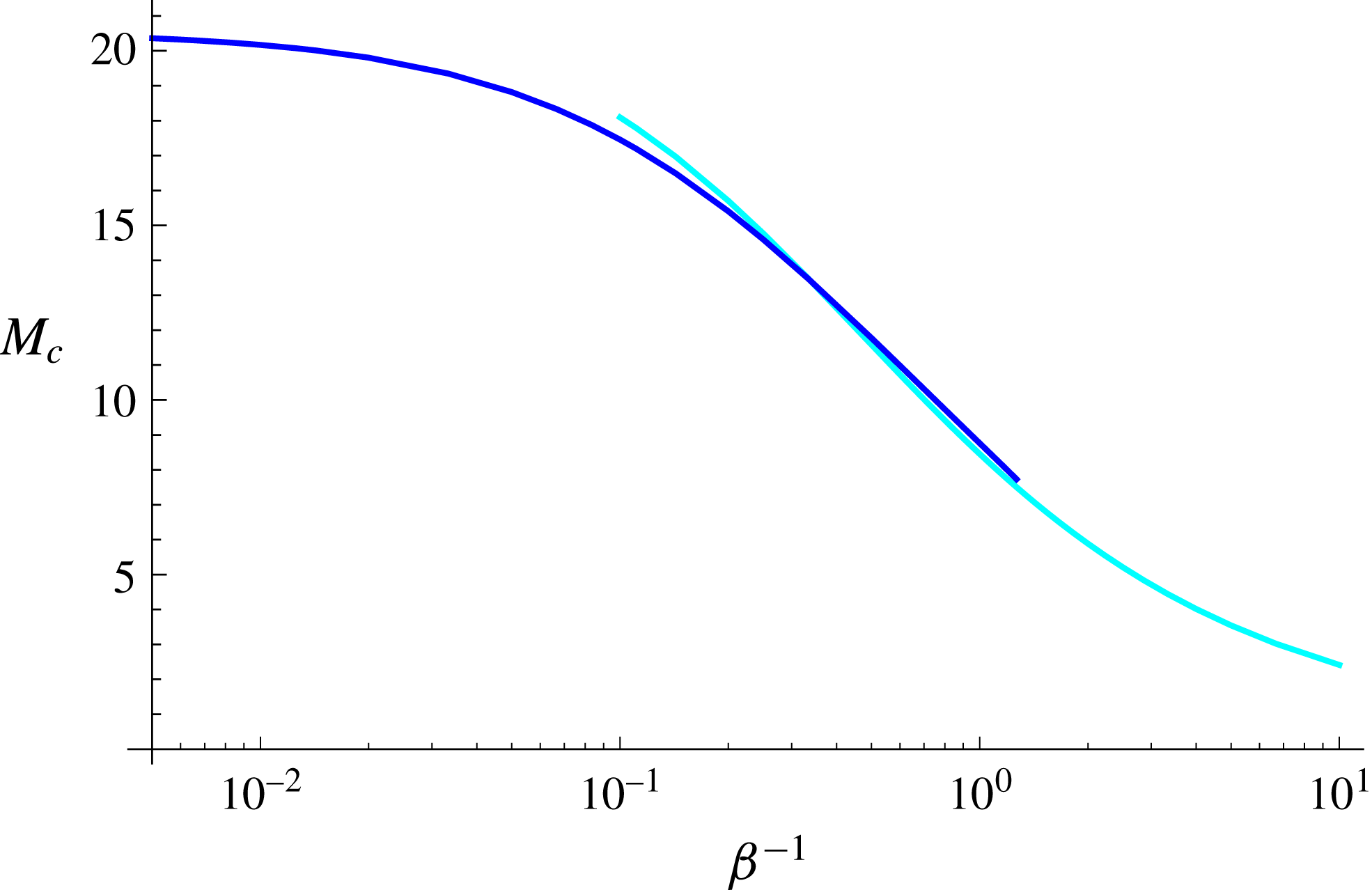
. For stationary longitudinal rolls, the minimal Marangoni number follows the translated power law
 $M_{m}\sim 20.2(\unicode[STIX]{x1D6FD}^{-1}+0.33)^{-0.61}$
for
 $Pr=1/2$
and
 $B=5$
.
3.2 Longitudinal travelling waves
For non-zero frequencies
 $\unicode[STIX]{x1D714}$
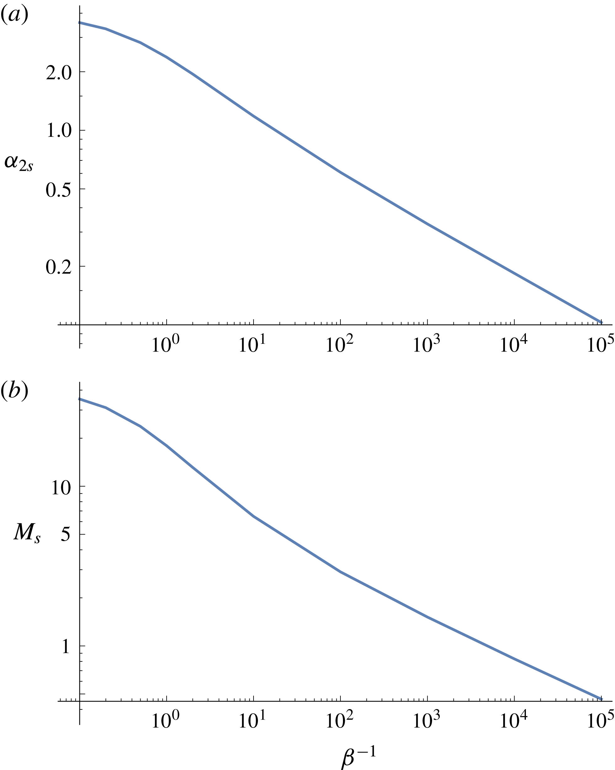
, the resulting instabilities are longitudinal travelling waves propagating in either of the normal directions to the mean flow. The growth rates come in complex conjugate pairs as seen in figure 3(b). The wavenumbers, for which these travelling waves exist, are bounded from above by a cutoff wavenumber
 $\unicode[STIX]{x1D6FC}_{2s}$
at a non-zero cutoff Marangoni number
 $M_{s}$
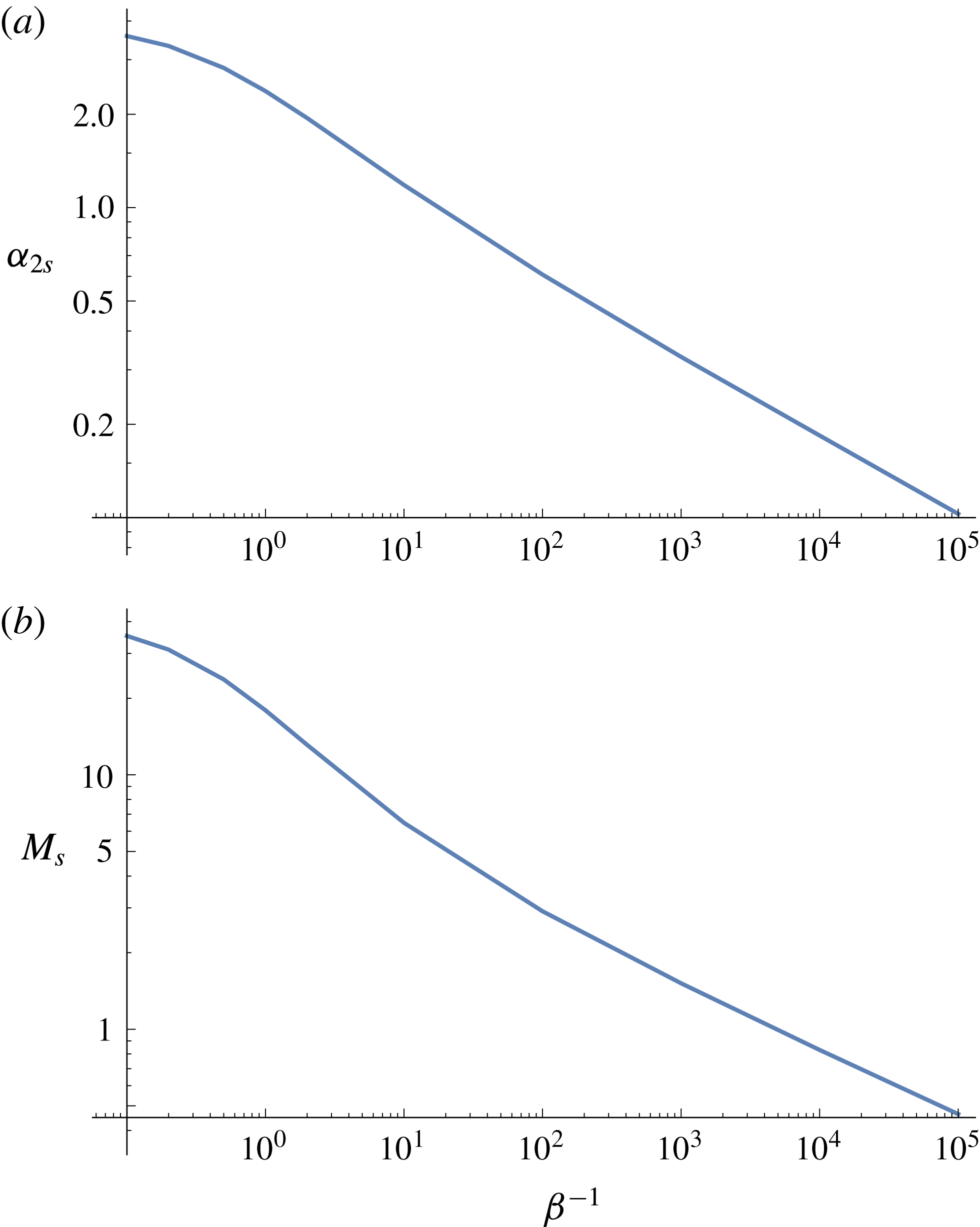
. Figure 8 shows
 $\unicode[STIX]{x1D6FC}_{2s}$
and
 $M_{s}$
as a function of
 $\unicode[STIX]{x1D6FD}^{-1}$
. Both
 $\unicode[STIX]{x1D6FC}_{2s}$
and
 $M_{s}$
decrease monotonically as
 $\unicode[STIX]{x1D6FD}^{-1}\rightarrow \infty$
, and a stability limit is identified as
 $\unicode[STIX]{x1D6FD}^{-1}\rightarrow \infty$
.
The cutoff wavenumber coincides with the minimal wavenumber for small enough
 $\unicode[STIX]{x1D6FD}^{-1}$
. Precisely, the minimum of each neutral curve, as seen in figure 3, occurs at
 $\unicode[STIX]{x1D6FC}=\unicode[STIX]{x1D6FC}_{2m}$
, where
 $\unicode[STIX]{x1D6FC}_{2m}<\unicode[STIX]{x1D6FC}_{2s}$
for large enough
 $\unicode[STIX]{x1D6FD}^{-1}$
, and
 $\unicode[STIX]{x1D6FC}_{2m}=\unicode[STIX]{x1D6FC}_{2s}$
otherwise. In the latter case, the most preferred wavenumber is exactly the cutoff wavenumber. Similarly to longitudinal rolls, the minimal Marangoni number for longitudinal travelling waves, as well as the associated wavenumber
 $\unicode[STIX]{x1D6FC}_{2m}$
, both decrease with
 $\unicode[STIX]{x1D6FD}^{-1}$
. That is, basal slip destabilizes the system.
Although not the preferred mode of instability, longitudinal travelling waves are close to the preferred mode of instability for low enough Prandtl numbers as seen in figure 5 for
 $B=0$
, both with and without basal slip. Oblique hydrothermal waves (modes for which
 $\unicode[STIX]{x1D6FC}_{1},\unicode[STIX]{x1D6FC}_{2}\neq 0$
and
 $\unicode[STIX]{x1D714}\neq 0$
) are preferred over strictly longitudinal travelling waves for this range of Prandtl numbers, although these oblique waves are near longitudinal. A similar observation can be made for larger Biot numbers, as seen in figure 6 for
 $B=5$
. Similarly to longitudinal rolls, increasing Biot numbers give rise to increasing Marangoni numbers.
The minimal Marangoni number and associated wavenumber for longitudinal waves is shown in figure 7 as a function of
 $\unicode[STIX]{x1D6FD}^{-1}$
for
 $Pr=1/2$
and
 $B=5$
. Although it is not a global minimum for any range of
 $\unicode[STIX]{x1D6FD}^{-1}$
, the minimal Marangoni number for longitudinal waves follows the translated power law
 $M_{m}\sim 19.8(\unicode[STIX]{x1D6FD}^{-1}+0.29)^{-0.51}$
.
Cutoff (
 $a$
) wavenumber and (
 $b$
) associated Marangoni number for longitudinal waves versus
 $\unicode[STIX]{x1D6FD}^{-1}$
. Parameters:
 $B=5,B_{l}=0,Pr=1/2$
.
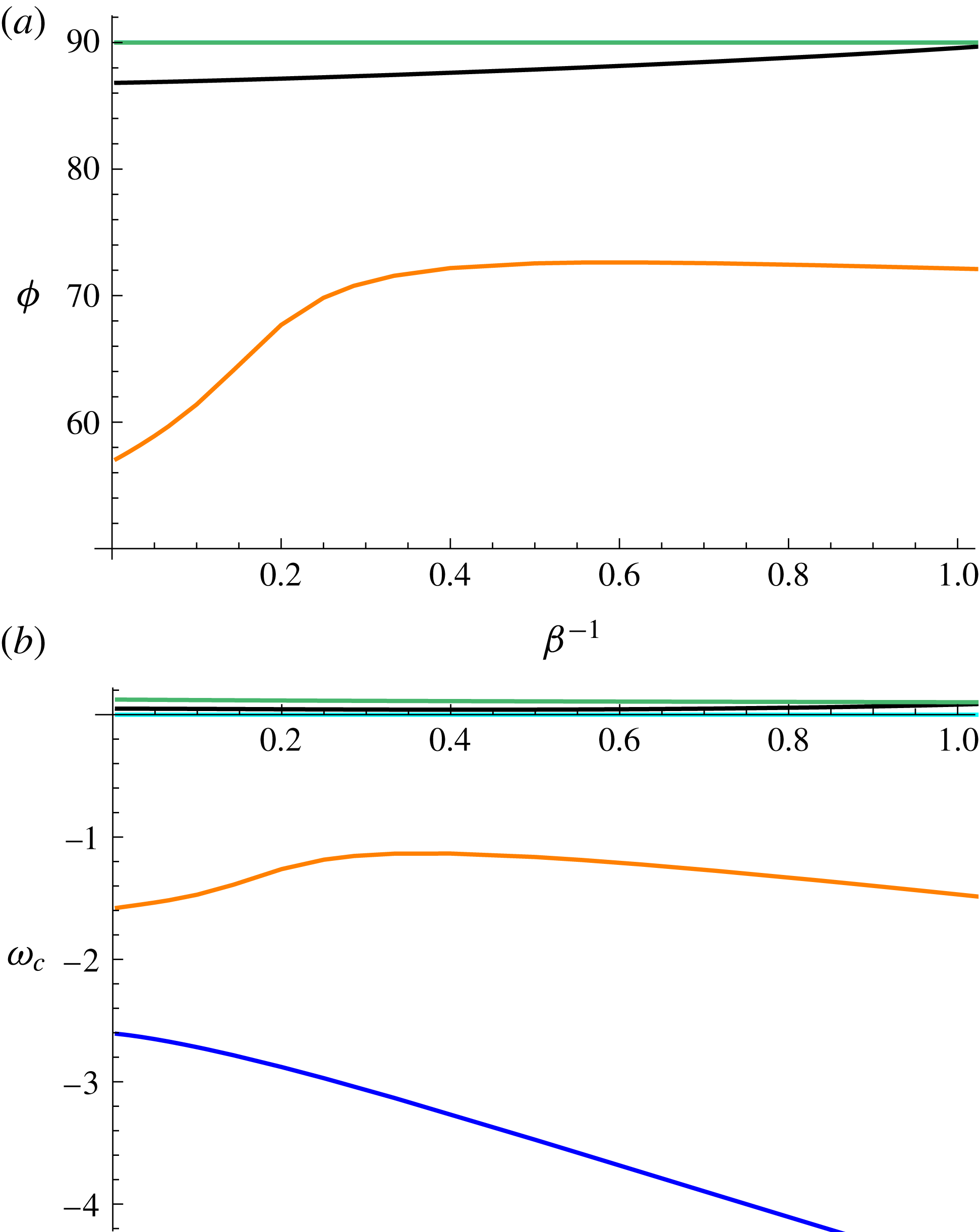
Critical (
 $a$
)
 $\unicode[STIX]{x1D719}$
and (
 $b$
)
 $\unicode[STIX]{x1D714}$
for
 $Pr=1/2$
,
 $B=5$
and
 $B_{l}=0$
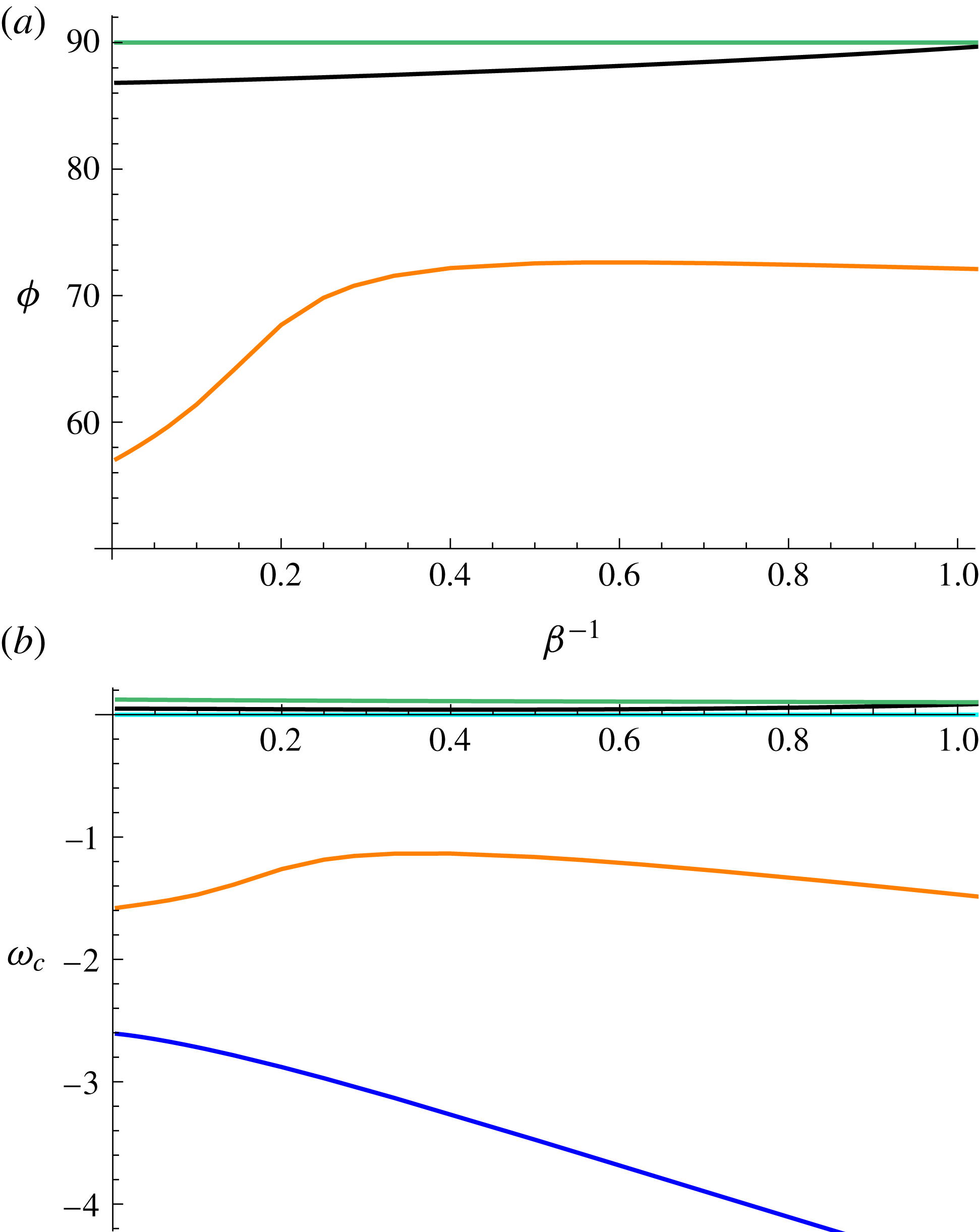
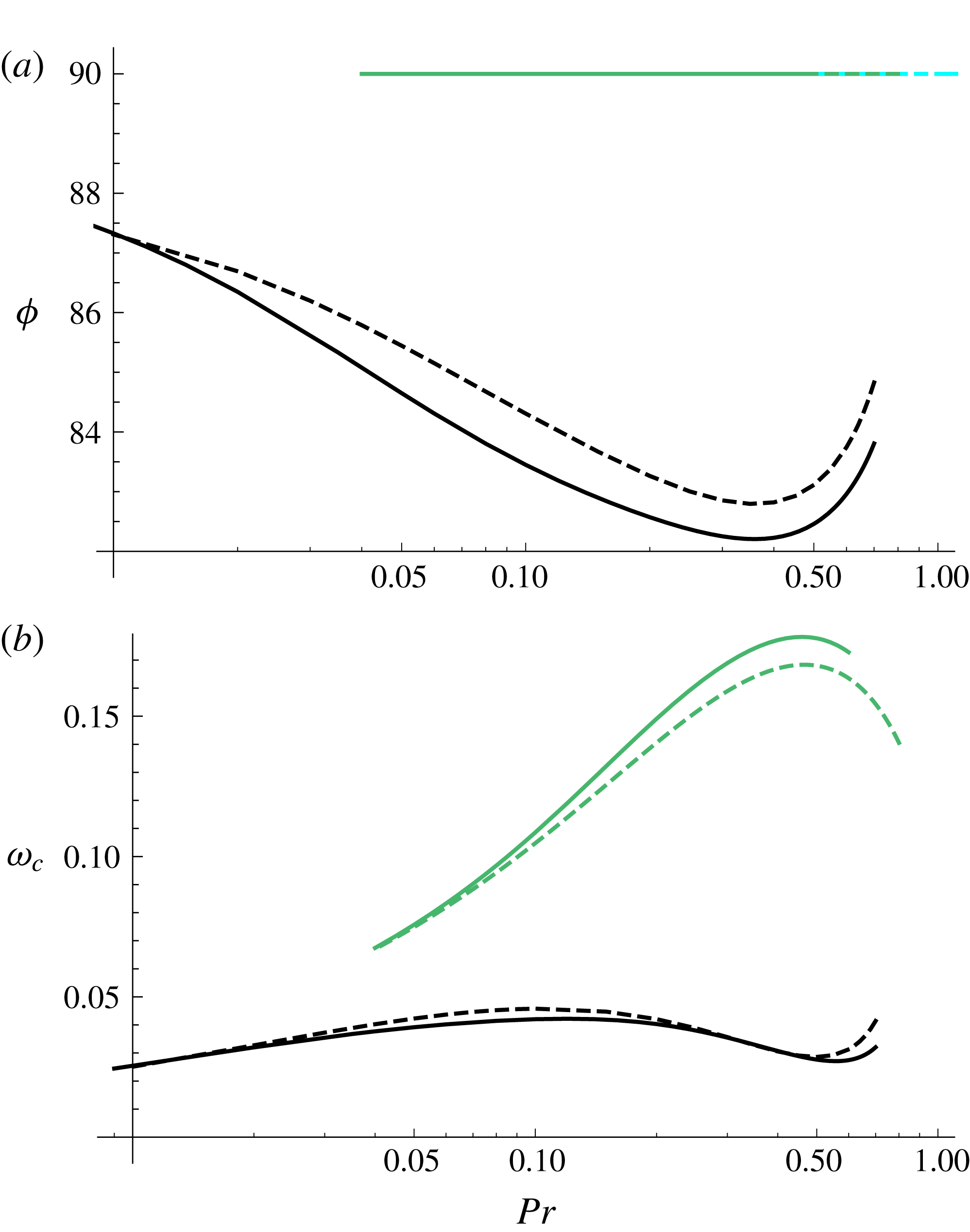
. Longitudinal rolls are shown in cyan, longitudinal waves are shown in green, oblique hydrothermal waves are shown in black and orange and two-dimensional hydrothermal waves are shown in blue.
Critical values of (
 $a$
)
 $\unicode[STIX]{x1D719}$
and (
 $b$
)
 $\unicode[STIX]{x1D714}$
, for
 $B=0$
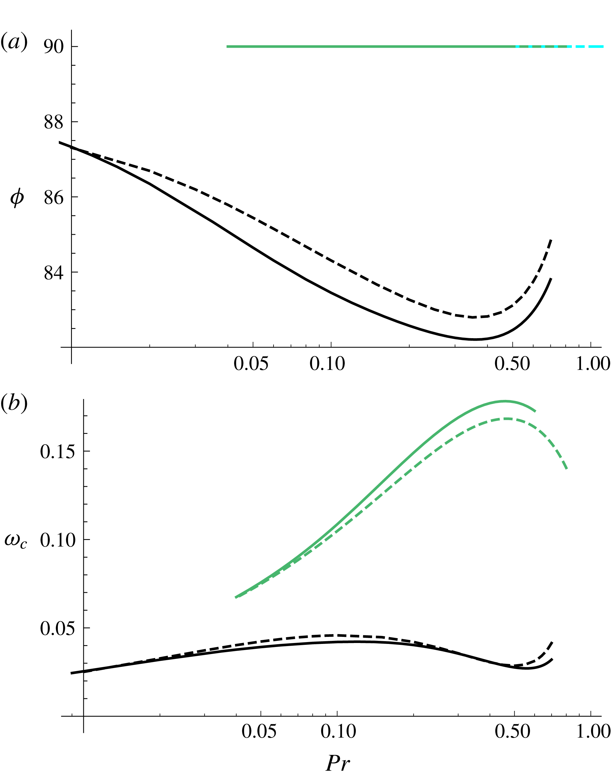
, in the no-slip limit (solid curves) and partial slip (dashed curves) for oblique hydrothermal waves (black), two-dimensional hydrothermal waves (blue), longitudinal rolls (cyan) and longitudinal waves (green). The preferred mode is given by the lowest value of
 $M$
for each
 $Pr$
. Slip destabilizes the system for all types of modes.
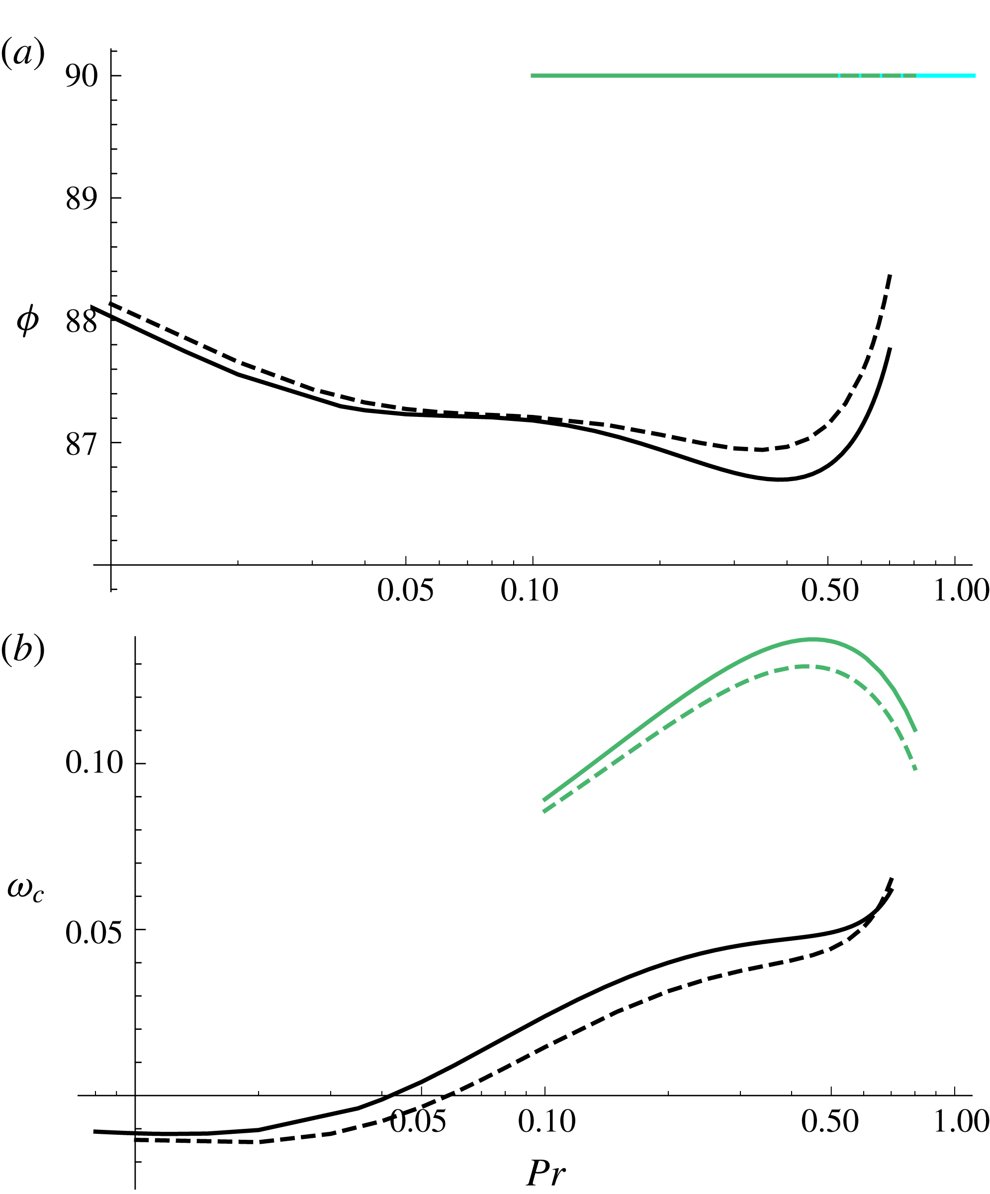
Critical values of (
 $a$
)
 $\unicode[STIX]{x1D719}$
and (
 $b$
)
 $\unicode[STIX]{x1D714}$
, for
 $B=5$
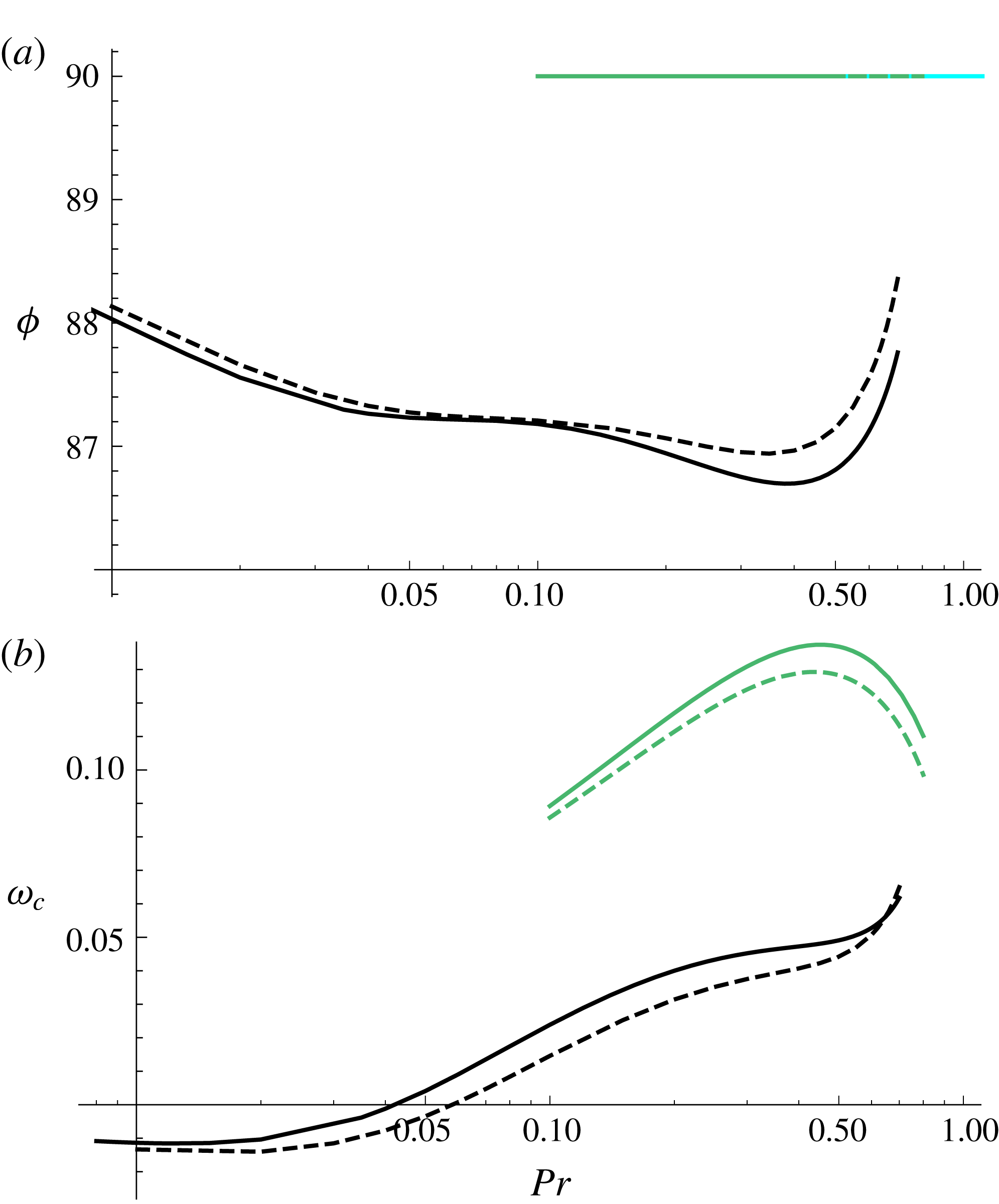
, in the no-slip limit (solid curves) and partial slip (dashed curves) for oblique hydrothermal waves (black), two-dimensional hydrothermal waves (blue), longitudinal rolls (cyan) and longitudinal waves (green). The preferred mode is given by the lowest value of
 $M$
for each
 $Pr$
.
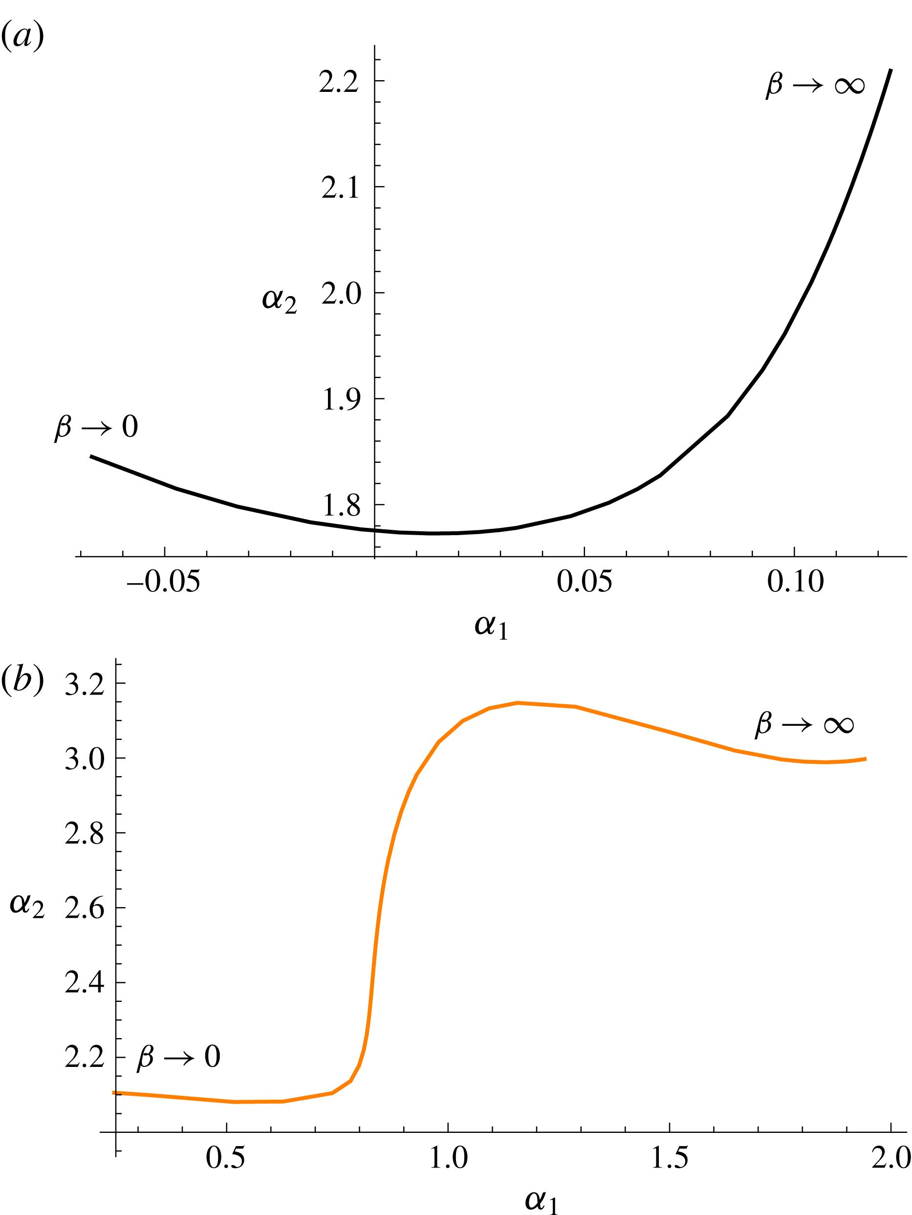
Critical wavevector for the two oblique modes for
 $Pr=1/2$
and
 $B=5$
and varying values of
 $\unicode[STIX]{x1D6FD}$
. The wavevector for the near-longitudinal mode is shown in (a).

4 Two-dimensional hydrothermal waves
Hydrothermal waves with
 $\unicode[STIX]{x1D6FC}_{2}=0$
and
 $\unicode[STIX]{x1D714}\neq 0$
(there is no steady bifurcation when
 $\unicode[STIX]{x1D6FC}_{2}=0$
) constitute a third mode of instability. These two-dimensional waves need not be the preferred mode of instability in all situations, although they are the preferred modes of instability for intermediate Prandtl numbers and small enough Biot numbers. For
 $B=0$
, this range of Prandtl numbers is approximately given by
 $0.6\lessapprox Pr\lessapprox 1.5$
without slip as seen in figure 5(a). This range narrows down as the slip parameter increases as seen in figure 14(a). At fixed
 $Pr$
and
 $B$
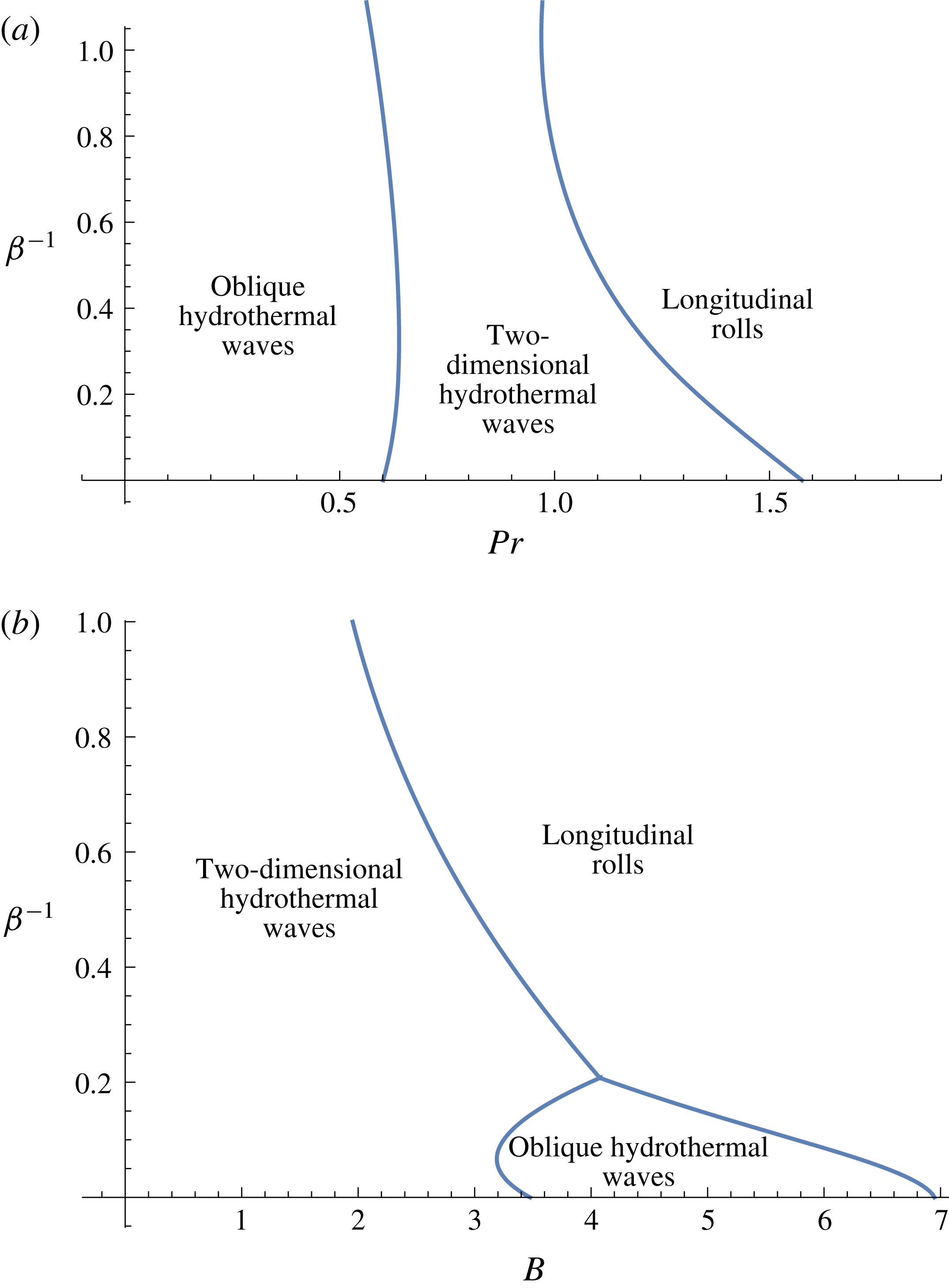
, it is common for two-dimensional hydrothermal waves to become no longer preferred when the slip parameter exceeds a critical value as seen in figure 13. Either oblique hydrothermal waves or longitudinal rolls are preferred for larger slip parameters. As seen illustratively in figure 5(a), the range of Prandtl numbers for which two-dimensional waves are preferred reduces to
 $0.63\lessapprox Pr\lessapprox 1.35$
when
 $\unicode[STIX]{x1D6FD}=5$
.
Similarly, as the Biot number increases, this range narrows down until two-dimensional hydrothermal waves are no longer the preferred mode of instability for large enough Biot numbers as seen in figure 14(b). This is an important qualitative change as
 $B$
increases, which occurs even though quantitative changes to longitudinal modes are small. Increasing basal slip reduces this range further. This can be observed in figure 6(a) for
 $B=5$
, where the neutral curve for two-dimensional hydrothermal waves is nowhere minimal in comparison to other modes. Instead, longitudinal rolls and oblique hydrothermal waves become preferred.
Despite parameter configurations in which two-dimensional waves are not the preferred mode of instability at a fixed Prandtl and Biot number, it is common for these waves to be almost preferable as the slip parameter increases as seen in figure 7(a). Figure 7(a) shows minimal Marangoni numbers for various modes for
 $Pr=1/2,B=5$
as a function of
 $\unicode[STIX]{x1D6FD}^{-1}$
, where oblique hydrothermal waves are preferred in the no-slip limit and for low slip, and two-dimensional hydrothermal waves are close to being preferred for high enough
 $\unicode[STIX]{x1D6FD}^{-1}$
.
The wavenumber associated with the minimal Marangoni number for two-dimensional hydrothermal waves is shown in figure 7(b) for
 $Pr=1/2$
and
 $B=5$
. The minimal Marangoni number for these two-dimensional waves follows the translated power law
 $M_{m}\sim 21.1(\unicode[STIX]{x1D6FD}^{-1}+0.35)^{-0.60}$
. The magnitude of the frequency of these two-dimensional waves increases almost linearly with the slip parameter as seen in figure 9.
5 Oblique hydrothermal waves
Modes with
 $\unicode[STIX]{x1D6FC}_{1}\neq 0$
,
 $\unicode[STIX]{x1D6FC}_{2}\neq 0$
and
 $\unicode[STIX]{x1D714}\neq 0$
, namely, oblique hydrothermal waves, are some of the most commonly seen modes of instability. These oblique waves form the preferred mode of instability for low Prandtl numbers. This is the case both with and without slip, although the Prandtl numbers required for these modes to dominate are higher (lower) with slip than in the no-slip limit for small (large) Biot numbers. For
 $B=0$
, the cutoff Prandtl number, indicating the upper bound on the Prandtl number for these modes to dominate, is given by
 $Pr\approx 0.6$
in the no-slip limit and
 $Pr\approx 0.63$
with partial slip, for
 $\unicode[STIX]{x1D6FD}=5$
, as seen in figure 5. This range of Prandtl numbers widens slightly for higher Biot numbers, to
 $Pr\approx 0.66$
in the no-slip limit and
 $Pr\approx 0.64$
under partial slip with
 $\unicode[STIX]{x1D6FD}=5$
. The preferred oblique hydrothermal waves are near longitudinal both with and without partial slip as seen in figure 10(a) for
 $B=0$
and figure 11(a) for
 $B=5$
. Although oblique hydrothermal waves may be preferred for fixed values of
 $Pr$
and
 $B$
in the no-slip limit, it is possible for these waves to become secondary to two-dimensional waves or longitudinal rolls as the slip parameter increases. This is seen in figure 14(b) at a fixed Prandtl number, where oblique waves are preferred for intermediate Biot numbers for small
 $\unicode[STIX]{x1D6FD}^{-1}$
, and cease to be preferred for slip parameters that exceed a critical value.
There are two distinct oblique hydrothermal waves, and depending on the slip parameter, either one or the other forms the preferred mode of instability. As seen in figure 7, the oblique hydrothermal wave that forms the preferred mode of instability in the no-slip limit for
 $Pr=1/2$
and
 $B=5$
remains preferred for low enough slip parameters up to a cutoff value
 $\unicode[STIX]{x1D6FD}^{-1}\approx 0.6$
, beyond which the other oblique hydrothermal wave is preferred. The magnitude of the frequency of the latter wave, which increases with slip for large enough
 $\unicode[STIX]{x1D6FD}^{-1}$
, is much greater than that of the former, as seen in figure 9(b).
The angle of inclination
 $\unicode[STIX]{x1D719}=(180/\unicode[STIX]{x03C0})\arctan (\unicode[STIX]{x1D6FC}_{2}/\unicode[STIX]{x1D6FC}_{1})$
of the critical wavevector of the near-two-dimensional oblique hydrothermal wave is shown in figure 9, in comparison with that of the other oblique hydrothermal wave, which remains near longitudinal for all slip parameters. It is interesting to note that these two modes approach each other, in the sense that the eigenvalues corresponding to the two modes approach each other with
 $\unicode[STIX]{x1D6FD}^{-1}$
, but the modes remain distinct. Figure 12 shows the wavevector in the
 $(\unicode[STIX]{x1D6FC}_{1},\unicode[STIX]{x1D6FC}_{2})$
-plane for both oblique hydrothermal waves as a function of the slip parameter. The near-longitudinal mode changes direction with
 $\unicode[STIX]{x1D6FD}$
.
As seen in figure 10(b) for
 $B=B_{l}=0$
, preferred oblique hydrothermal waves, which in this case are near longitudinal, travel against the base flow for all Prandtl numbers under the no-slip limit (which follows from the definition of
 $\unicode[STIX]{x1D714}$
and its positivity in figure 10
b). This remains the case under partial slip and the frequencies increase for large enough Prandtl numbers. However, this behaviour reverses for larger Biot numbers and small enough Prandtl numbers, as seen in figure 11(b). Oblique waves travel with the flow in this case, and the range of Prandtl numbers for which these waves travel with the flow expands under partial slip.
Critical Marangoni number versus
 $\unicode[STIX]{x1D6FD}^{-1}$
for
 $B=B_{l}=0$
and
 $Pr=1.2$
. Two-dimensional waves (blue) and longitudinal rolls (cyan) are preferred for small, respectively, large
 $\unicode[STIX]{x1D6FD}^{-1}$
.
Regime diagram showing the appearance of oblique hydrothermal waves, two-dimensional hydrothermal waves and longitudinal rolls in (
 $a$
)
 $(Pr,\unicode[STIX]{x1D6FD}^{-1})$
space for
 $B=B_{l}=0$
and (
 $b$
)
 $(B,\unicode[STIX]{x1D6FD}^{-1})$
space for
 $Pr=0.65$
and
 $B_{l}=0$
.
6 Conclusions
We have investigated the onset of two- and three-dimensional hydrothermal waves, longitudinal rolls and longitudinal travelling waves in a low-capillary-number horizontal liquid layer of arbitrary depth with a lower boundary that allows for slip. Hydrothermal waves result from an imposed horizontal temperature gradient along the upper, liquid–gas interface. In dimensional terms, the wavelengths of the generated instabilities are comparable to the layer depth. We find that the selection of preferred mode of instability depends intricately on the basal slip parameter.
We find that partial slip destabilizes the system for all modes of instability and reduces the occurrence of longitudinal travelling waves. The minimum Marangoni number required for the onset of instability decreases monotonically with
 $\unicode[STIX]{x1D6FD}^{-1}$
for all these modes. Specifically, the minimum Marangoni number follows a translated power law of the type
 $M_{m}\sim a(\unicode[STIX]{x1D6FD}^{-1}+b)^{-c}$
for each of these modes, where
 $a,b,c$
are positive constants.
The band of wavenumbers for which longitudinal travelling waves appear narrows down until this mode of instability fully disappears in favour of longitudinal rolls in the limit of free slip. The minimal Marangoni number required for the onset of longitudinal rolls as well as the associated wavenumber both decrease monotonically with the slip parameter. Longitudinal rolls are the preferred modes of instability for large enough Prandtl numbers both with and without slip, although lower Prandtl numbers are required for these modes to be preferred under partial slip. That is, higher slip parameters promote the occurrence of longitudinal rolls for a widening range of Prandtl numbers as seen in figure 14. Similarly, increasing Biot numbers give rise to wider ranges of Prandtl numbers for which longitudinal rolls are the dominant mode of instability. The critical wavenumber for longitudinal rolls decreases monotonically with
 $Pr$
, both with and without partial slip, until the system selects long wave instabilities near a critical Prandtl number under no heat flux and partial slip. Longitudinal rolls become favourable also for low Prandtl numbers, as long as
 $B$
is large enough. This range of Biot numbers expands with increasing slip.
Two-dimensional hydrothermal waves are the preferred mode of instability for intermediate Prandtl numbers and low Biot numbers. The range of Prandtl numbers for which two-dimensional hydrothermal waves are preferred reduces with the slip parameter, and these waves tend to be selected by the system for lower Prandtl numbers under partial slip as seen in figure 14(b). The range of Biot numbers for which these waves are preferred similarly reduces with increasing slip. It is, however, common for the Marangoni number for two-dimensional hydrothermal waves to approach the critical Marangoni number as the slip parameter increases, while
 $Pr$
and
 $B$
are fixed.
The system selects oblique hydrothermal waves as the preferred form of instability for low Prandtl numbers. For small
 $\unicode[STIX]{x1D6FD}^{-1}$
, partial slip reduces (expands) the range of Prandtl numbers required for these waves to be preferred for large (small) Biot numbers, while increasing Biot numbers slightly expand this range. As
 $\unicode[STIX]{x1D6FD}^{-1}$
increases further, the range of Prandtl numbers reduces further, in favour of the occurrence of two-dimensional hydrothermal waves. It is common to see oblique hydrothermal waves for intermediate Biot numbers and for low enough slip parameters
 $\unicode[STIX]{x1D6FD}^{-1}$
at a fixed value of
 $Pr$
, as seen in figure 14(b). These oblique waves are no longer preferred for slip parameters that exceed a critical value. There are two distinct types of oblique hydrothermal waves and the system selects either one or the other of these oblique waves depending on the slip parameter. One of these modes is near longitudinal for all slip parameters. These near-longitudinal oblique hydrothermal waves are preferred for low-slip parameters up to a cutoff value of
 $\unicode[STIX]{x1D6FD}^{-1}$
. The secondary oblique hydrothermal wave, of much higher frequency, becomes preferred for larger slip parameters.
Acknowledgement
This work is supported by the National Institute of Standards and Technology [grant number 70NANB14H012] as part of the Center for Hierarchical Material Design (CHiMaD).