1 Introduction
When a solute-stratified fluid has an imposed horizontal temperature difference beyond the critical value, the fluid on the hot (cold) side will rise (sink) until it reaches a height (depth)
 $d=\unicode[STIX]{x1D6FC}\unicode[STIX]{x0394}T/(-\unicode[STIX]{x1D6FD}\,\text{d}S/\text{d}z)$
in which
 $T$
is temperature,
 $S$
is salinity,
 $\unicode[STIX]{x1D6FC}=-\unicode[STIX]{x1D70C}_{0}^{-1}(\unicode[STIX]{x2202}\unicode[STIX]{x1D70C}/\unicode[STIX]{x2202}T)$
and
 $\unicode[STIX]{x1D6FD}=\unicode[STIX]{x1D70C}_{0}^{-1}(\unicode[STIX]{x2202}\unicode[STIX]{x1D70C}/\unicode[STIX]{x2202}S)$
(Chen, Briggs & Wirtz Reference Chen, Briggs and Wirtz1971). Then the fluid turns horizontally to the bulk fluid, forming a horizontal convecting layer. Within the layer, the hot and solute-rich fluid moves along the upper horizontal boundary and the cold and solute-poor fluid moves along the lower horizontal boundary, creating a situation conducive to the onset of a salt-finger instability (Thorpe, Hutt & Soulsby Reference Thorpe, Hutt and Soulsby1969; Chen et al.
Reference Chen, Briggs and Wirtz1971; Wirtz, Briggs & Chen Reference Wirtz, Briggs and Chen1972; Malki-Epshtein, Phillips & Huppert Reference Malki-Epshtein, Phillips and Huppert2004). The salt-finger instability, a secondary instability occurring in the convecting layer, may appear with two different instability modes. The transverse mode (see figures 2 and 9 of Chan, Chen & Chen Reference Chan, Chen and Chen2002) takes the form of rolls with their axes perpendicular to the transverse plane (the
 $x$
–
 $z$
plane, parallel to the imposed temperature gradient and the gravity vector) and the longitudinal mode (see figures 3 and 10 of Chan et al.
Reference Chan, Chen and Chen2002) with their axes perpendicular to the longitudinal plane (the
 $y$
–
 $z$
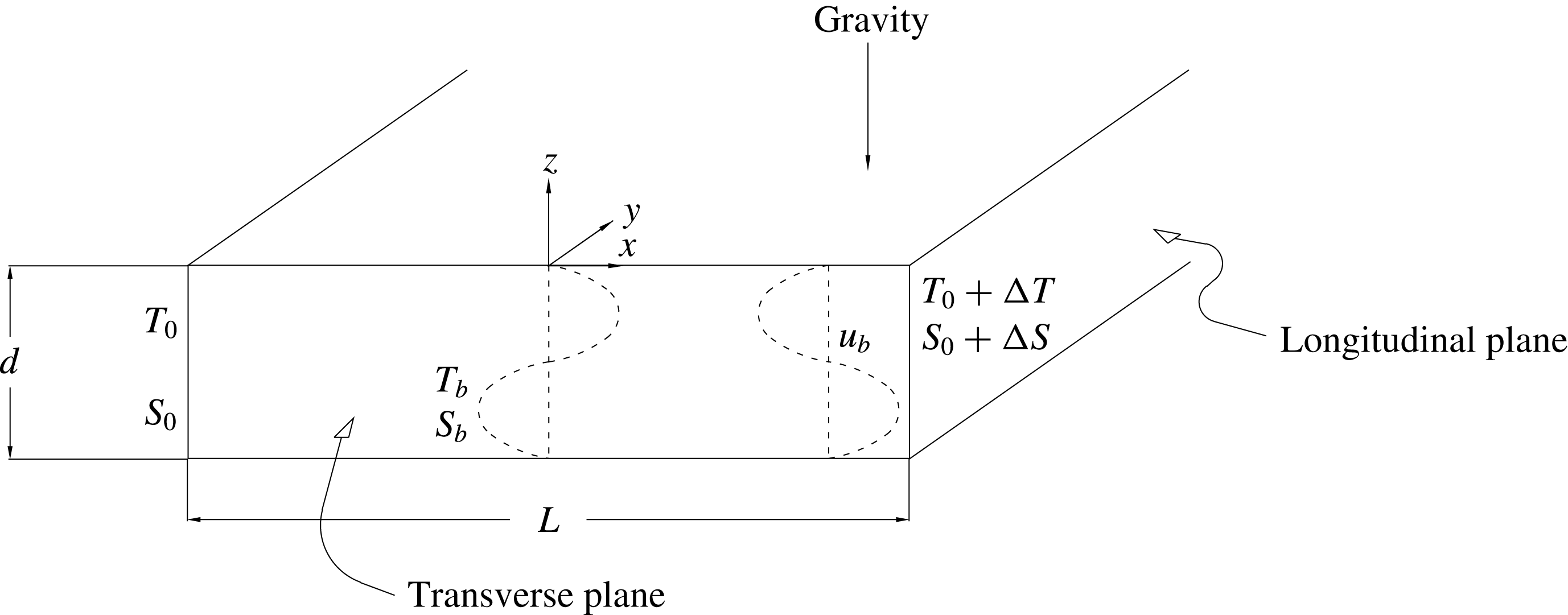
plane, perpendicular with the imposed temperature gradient and the gravity vector). See the schematic drawing in figure 1.
A schematic description of the physical domain considered. The transverse plane is aligned with the
 $x$
–
 $z$
plane and the longitudinal plane with the
 $y$
–
 $z$
plane. The box is heated on the longitudinal plane on the right and cooled on the left. The gravity points downwards in the negative-
 $z$
direction. The convecting layer is confined to the region having a depth
 $d$
and a length
 $L$
. The schematic descriptions of the basic state of the flow
 $\boldsymbol{u}_{b}$
at an arbitrary
 $x$
and those of the temperature
 $T_{b}$
and the solute
 $S_{b}$
at
 $x=0$
are also shown, which are adapted from the figure 6 of Chan et al. (Reference Chan, Chen and Chen2002).

Both the transverse and longitudinal modes could have been observed in experiments. For example, Chen & Chen (Reference Chen and Chen1997) conducted experiments in which a temperature difference of
 $7.3\,^{\circ }\text{C}$
across a tank (exceeding the critical value of
 $6.5\,^{\circ }$
C by Thorpe et al.
Reference Thorpe, Hutt and Soulsby1969) was applied impulsively. As shown in their figure 3, an array of horizontal convecting layers formed a few minutes later. In each layer, as observed via particle traced images from the top of experimental box, a row of counter-rotating vortices occurred virtually simultaneously with the layer formation and advanced with a uniform front. These vortices were found having a wavelength approximately half of the depth of convecting layer and an axis perpendicular to the longitudinal plane, commonly recognized to be the longitudinal mode of the secondary instability (Kerr Reference Kerr2000; Chan et al.
Reference Chan, Chen and Chen2002). The uniform front, as observed via shadowgraphs on the transverse plane, could be the boundary of a vortex having a wavelength approximately the height of convecting layer and an axis perpendicular to the transverse plane, two typical features of the transverse mode.
When the temperature gradient was imposed gradually, as shown in the figures 5 and 6 of Chen & Chen (Reference Chen and Chen1997) where the temperature difference was increased by
 $2\,^{\circ }\text{C}$
every hour up to
 $8\,^{\circ }\text{C}$
, the formation of convecting layers was observed to be a result of the successive generation of vortices. These vortices, like those found in the impulsive-started experiment above, had a wavelength approximately the height of convecting layer and an axis perpendicular to the transverse plane, which accordingly were speculated to be evidence of a transverse mode. Within the vortices, a row of counter-rotating vortices (or the longitudinal modes) occurred almost simultaneously with the onset of the transverse mode. These experimental observations of Chen & Chen (Reference Chen and Chen1997) concluded that, regardless of the way the temperature difference was imposed, the formation of a convecting layer occurred almost simultaneously with the onset of both the longitudinal and transverse modes. However, since the experimental conditions were well above the critical values so that the flows observed were fully nonlinear, it is indeed very difficult to rationalize by experiments the reasons as well as the conditions triggering these convective flows.
Theoretical approaches accordingly were implemented. To investigate the stability of a convecting layer, Kerr (Reference Kerr1992) considered a double-diffusive interleaving layer formed in a fluid with vertical temperature and solute gradients and imposed horizontal temperature and solute gradients and performed a two-dimensional stability analysis for the secondary instability of the layer. Later, stimulated by the experiments of Chen & Chen (Reference Chen and Chen1997) and Biello (Reference Biello1997) that three-dimensional secondary flows indeed appear in the convecting layer while the critical conditions of the onset of secondary flows were not clearly identified, Kerr (Reference Kerr2000) extended his earlier two-dimensional analysis to a three-dimensional one. In order to make the analysis tractable, he focused on the stability of the fastest growing mode parallel to the convecting flow and concluded that the longitudinal mode taking the form of a circular vortex aligned with the convecting flow can be the most unstable. He also showed that the growth rate of the transverse mode is close to that of the longitudinal mode, implying that the stability boundaries of the two modes can be close.
To examine the stability boundaries of the two modes in more detail, Chan et al. (Reference Chan, Chen and Chen2002) conducted a linear stability analysis for both the longitudinal and transverse modes separately, which was essentially a two-dimensional analysis. Their basic flow was slightly different from Kerr (Reference Kerr1992, Reference Kerr2000), which was a convecting layer having a horizontally linear temperature and solute gradients while both the temperature and the solute on the top and bottom were assumed to be the same (see figure 6 of Chan et al.
Reference Chan, Chen and Chen2002). Their results showed that, for the case
 $Le=3$
, the stability boundaries of the two modes have an obvious difference. For the case
 $Le=100$
, they showed only the stability boundary of the longitudinal mode due to the difficulty of getting a convergent solution for the transverse mode. Later, Chen & Chan (Reference Chen and Chan2010) extended their analyses by including the surface tension effect on the upper boundary of a convecting layer and concluded that both transverse and longitudinal modes become more unstable under the influence of surface tension.
The studies discussed above indicate that both experimental and theoretical studies are not able to offer a clear and conclusive result to illustrate the stability characteristics of the transverse and longitudinal modes. The lack of a conclusive result, as argued by Kerr (Reference Kerr1992), can be due to the fact that the instability is three-dimensional while most experimental observations have been pursued on the planes either parallel or perpendicular to the temperature gradient, which tended not to show much evidence of three-dimensional instabilities. Similarly, Chen & Chen (Reference Chen and Chen1997) speculated that the analyses based on a two-dimensional flow structure may result in a grossly under-predicted outcome. After performing both experimental and theoretical investigations, Chan et al. (Reference Chan, Chen and Chen2002) suggested also that a three-dimensional simulation shall be performed to prevent the loss of information about the potential instability modes moving in directions oblique to either the transverse or the longitudinal plane.
In the present study, we perform a three-dimensional stability analysis for the convecting layer considered by Chan et al. (Reference Chan, Chen and Chen2002) and examine in detail the stability boundaries of the transverse and longitudinal modes and any possible mode moving in arbitrary directions. We first repeat the two-dimensional stability analysis of Chan et al. (Reference Chan, Chen and Chen2002), seeking stability maps for both
 $Le=3$
and 100, and then pursue a three-dimensional stability analysis to look for a potential instability mode moving in arbitrary directions in the
 $x$
–
 $y$
plane. In the following, the physical configuration of the basic state and its solution are given in § 2, the mathematical formulation and the numerical scheme are illustrated in § 3, the results of the stability analysis are elucidated and discussed in § 4 for the two-dimensional analysis and in § 5 for the three-dimensional analysis. Finally, in § 6 the discussion is given and the conclusion is summarized.
2 The physical configuration and the basic state solution
Consider a convecting layer of height
 $d$
and length
 $L$
shown in the transverse plane of figure 1. The flow on the upper (lower) half of the layer moves away from the hot (cold) wall, containing warmer (colder) and solute-rich (-poor) fluid while losing (gaining) heat and solute to (from) the counter-rotating layer above (below). Along both horizontal boundaries, the flow velocity is assumed zero and both the temperature and the solute decrease linearly from the hot wall to the cold wall. The temperature difference is the value imposed in the experiment, the solute difference is approximated by the solute difference between the bottom and the top of the tank divided by the number of convecting layers. Within the layer, based on the measurements of Chen & Chen (Reference Chen and Chen1997), both the vertical solute and temperature differences can be assumed zero.
More specifically, as considered by Chan et al. (Reference Chan, Chen and Chen2002), a shallow horizontal layer of thickness
 $d$
and length
 $L$
is considered. In such a layer, the temperature and solute concentration are maintained at
 $T_{0}$
and
 $S_{0}$
at the left wall and
 $T_{0}+\unicode[STIX]{x0394}T$
and
 $S_{0}+\unicode[STIX]{x0394}S$
at the right wall. In the present study, both
 $T_{0}$
and
 $S_{0}$
are considered to be zero. Along the upper and lower boundary, the distributions of temperature and solute concentration are linear with constant slopes
 $\unicode[STIX]{x1D6FE}=\unicode[STIX]{x0394}T/L$
and
 $\unicode[STIX]{x1D6FE}_{s}=\unicode[STIX]{x0394}S/L$
respectively. To render the governing equations non-dimensional, we take
 $d$
,
 $d^{2}/\unicode[STIX]{x1D708}$
,
 $g\unicode[STIX]{x1D6FC}\unicode[STIX]{x1D6FE}d^{3}/\unicode[STIX]{x1D708}$
,
 $\unicode[STIX]{x1D70C}_{0}(g\unicode[STIX]{x1D6FC}\unicode[STIX]{x1D6FE}d^{3}/\unicode[STIX]{x1D708})^{2}$
,
 $\unicode[STIX]{x1D6FE}d$
and
 $\unicode[STIX]{x1D6FE}_{s}d$
as the characteristic length, time, velocity, pressure, temperature and solute concentration, respectively. The non-dimensional governing equations are
 $$\begin{eqnarray}\displaystyle & \displaystyle \unicode[STIX]{x1D735}\boldsymbol{\cdot }\boldsymbol{u}=0, & \displaystyle\end{eqnarray}$$
 $$\begin{eqnarray}\displaystyle & \displaystyle \frac{\unicode[STIX]{x2202}\boldsymbol{u}}{\unicode[STIX]{x2202}t}+Gr\boldsymbol{u}\boldsymbol{\cdot }\unicode[STIX]{x1D735}\boldsymbol{u}=-Gr\unicode[STIX]{x1D735}P+\unicode[STIX]{x1D6FB}^{2}\boldsymbol{u}+\left(T-\frac{Gs}{Gr}S\right)g\boldsymbol{k}, & \displaystyle\end{eqnarray}$$
 $$\begin{eqnarray}\displaystyle & \displaystyle Pr\frac{\unicode[STIX]{x2202}T}{\unicode[STIX]{x2202}t}+GrPr\boldsymbol{u}\boldsymbol{\cdot }\unicode[STIX]{x1D735}T=\unicode[STIX]{x1D6FB}^{2}T, & \displaystyle\end{eqnarray}$$
 $$\begin{eqnarray}\displaystyle & \displaystyle LePr\frac{\unicode[STIX]{x2202}S}{\unicode[STIX]{x2202}t}+LeGrPr\boldsymbol{u}\boldsymbol{\cdot }\unicode[STIX]{x1D735}S=\unicode[STIX]{x1D6FB}^{2}S. & \displaystyle\end{eqnarray}$$
In above equations,
 $\boldsymbol{u}=(u,v,w)$
is the velocity vector, the Boussinesq approximation is applied and the thermal Grashof number
 $Gr$
, the solute Grashof number
 $Gs$
, the Prandtl number
 $Pr$
and the Lewis number
 $Le$
are defined respectively as
 $$\begin{eqnarray}\displaystyle Gr=\frac{g\unicode[STIX]{x1D6FC}\unicode[STIX]{x0394}Td^{3}}{\unicode[STIX]{x1D708}^{2}}\frac{d}{L},\quad Gs=\frac{g\unicode[STIX]{x1D6FD}\unicode[STIX]{x0394}Sd^{3}}{\unicode[STIX]{x1D708}^{2}}\frac{d}{L},\quad Pr=\frac{\unicode[STIX]{x1D708}}{\unicode[STIX]{x1D705}}\quad \text{and}\quad Le=\frac{\unicode[STIX]{x1D705}}{\unicode[STIX]{x1D705}_{s}}, & & \displaystyle\end{eqnarray}$$
where
 $\unicode[STIX]{x1D708}$
is the kinematic viscosity,
 $\unicode[STIX]{x1D705}$
is the thermal diffusivity and
 $\unicode[STIX]{x1D705}_{s}$
is the mass diffusivity. Both the top and bottom boundaries are assumed rigid and the boundary conditions are
 $$\begin{eqnarray}\displaystyle \boldsymbol{u}=0,\quad T=x,\quad S=x\quad \text{at}~z=\pm {\textstyle \frac{1}{2}}. & & \displaystyle\end{eqnarray}$$
We assume that the convecting layer is a steady parallel flow such that
 $\boldsymbol{u}_{b}=(u_{b}(z),0,0)$
,
 $T_{b}=T_{b}(x,z)$
and
 $S_{b}=S_{b}(x,z)$
. The basic solution can be obtained by solving (2.1)–(2.6) as follows
 $$\begin{eqnarray}\displaystyle & \displaystyle u_{b}=\frac{1}{6}\left(1-\frac{Gs}{Gr}\right)z\left(z^{2}-\frac{1}{4}\right), & \displaystyle\end{eqnarray}$$
 $$\begin{eqnarray}\displaystyle & \displaystyle T_{b}=x+\frac{GrPr}{6}\left(1-\frac{Gs}{Gr}\right)\left(\frac{1}{20}z^{5}-\frac{1}{24}z^{3}+\frac{7}{960}z\right), & \displaystyle\end{eqnarray}$$
 $$\begin{eqnarray}\displaystyle & \displaystyle S_{b}=x+\frac{LeGrPr}{6}\left(1-\frac{Gs}{Gr}\right)\left(\frac{1}{20}z^{5}-\frac{1}{24}z^{3}+\frac{7}{960}z\right). & \displaystyle\end{eqnarray}$$
In deriving (2.7), it is assumed that the basic state velocity profile is anti-symmetric with respect to
 $z=0$
so that the parallel flow features measured by the experiment of Chen & Chen (Reference Chen and Chen1997) can be satisfied. As a result, the term
 $-4C(z^{2}-1/4)$
originally in (2.7) vanishes by assuming the constant
 $C$
to be zero. Consequently, (2.7)–(2.9) are obtained to be exactly the same with those of Chan et al. (Reference Chan, Chen and Chen2002), as shown in figure 6 of Chan et al. (Reference Chan, Chen and Chen2002). In these profiles, one may find that there are two local maxima in the velocity profile located at
 $z=\pm 0.284$
and another two maxima located at
 $z=\pm 0.259$
in both the temperature and solute profiles.
3 The small perturbation equations and the numerical method
We pursue a linear stability analysis for (2.1)–(2.6) based on the basic state (2.7)–(2.9) by applying
 $u=u_{b}+u^{\prime }$
,
 $v=v^{\prime }$
,
 $w=w^{\prime }$
,
 $p=p_{b}+p^{\prime }$
,
 $T=T_{b}+T^{\prime }$
and
 $S=S_{b}+S^{\prime }$
, yielding the linearized small perturbation equations
 $$\begin{eqnarray}\displaystyle & \displaystyle \frac{\unicode[STIX]{x2202}u^{\prime }}{\unicode[STIX]{x2202}x}+\frac{\unicode[STIX]{x2202}v^{\prime }}{\unicode[STIX]{x2202}y}+\frac{\unicode[STIX]{x2202}w^{\prime }}{\unicode[STIX]{x2202}z}=0, & \displaystyle\end{eqnarray}$$
 $$\begin{eqnarray}\displaystyle & \displaystyle \frac{\unicode[STIX]{x2202}u^{\prime }}{\unicode[STIX]{x2202}t}+Gr\left(u_{b}\frac{\unicode[STIX]{x2202}u^{\prime }}{\unicode[STIX]{x2202}x}+w^{\prime }\frac{\unicode[STIX]{x2202}u_{b}}{\unicode[STIX]{x2202}z}\right)=-Gr\frac{\unicode[STIX]{x2202}p^{\prime }}{\unicode[STIX]{x2202}x}+\unicode[STIX]{x1D6FB}^{2}u^{\prime }, & \displaystyle\end{eqnarray}$$
 $$\begin{eqnarray}\displaystyle & \displaystyle \frac{\unicode[STIX]{x2202}v^{\prime }}{\unicode[STIX]{x2202}t}+Gru_{b}\frac{\unicode[STIX]{x2202}v^{\prime }}{\unicode[STIX]{x2202}x}=-Gr\frac{\unicode[STIX]{x2202}p^{\prime }}{\unicode[STIX]{x2202}y}+\unicode[STIX]{x1D6FB}^{2}v^{\prime }, & \displaystyle\end{eqnarray}$$
 $$\begin{eqnarray}\displaystyle & \displaystyle \frac{\unicode[STIX]{x2202}w^{\prime }}{\unicode[STIX]{x2202}t}+Gru_{b}\frac{\unicode[STIX]{x2202}w^{\prime }}{\unicode[STIX]{x2202}x}=-Gr\frac{\unicode[STIX]{x2202}p^{\prime }}{\unicode[STIX]{x2202}z}+\unicode[STIX]{x1D6FB}^{2}w^{\prime }+T^{\prime }-\frac{Gs}{Gr}S^{\prime }, & \displaystyle\end{eqnarray}$$
 $$\begin{eqnarray}\displaystyle & \displaystyle Pr\frac{\unicode[STIX]{x2202}T^{\prime }}{\unicode[STIX]{x2202}t}+GrPr\left(u_{b}\frac{\unicode[STIX]{x2202}T^{\prime }}{\unicode[STIX]{x2202}x}+u^{\prime }+w^{\prime }\frac{\unicode[STIX]{x2202}T_{b}}{\unicode[STIX]{x2202}z}\right)=\unicode[STIX]{x1D6FB}^{2}T^{\prime }, & \displaystyle\end{eqnarray}$$
 $$\begin{eqnarray}\displaystyle & \displaystyle LePr\frac{\unicode[STIX]{x2202}S^{\prime }}{\unicode[STIX]{x2202}t}+LeGrPr\left(u_{b}\frac{\unicode[STIX]{x2202}S^{\prime }}{\unicode[STIX]{x2202}x}+u^{\prime }+w^{\prime }\frac{\unicode[STIX]{x2202}S_{b}}{\unicode[STIX]{x2202}z}\right)=\unicode[STIX]{x1D6FB}^{2}S^{\prime }, & \displaystyle\end{eqnarray}$$
and the boundary conditions
 $$\begin{eqnarray}\displaystyle u^{\prime }=v^{\prime }=w^{\prime }=T^{\prime }=S^{\prime }=0\quad \text{at}~z=\pm {\textstyle \frac{1}{2}}. & & \displaystyle\end{eqnarray}$$
3.1 Three-dimensional equations for general modes
For three-dimensional stability analysis, the normal mode expansion is given as
 $$\begin{eqnarray}\displaystyle \left(\begin{array}{@{}c@{}}u^{\prime }\\ v^{\prime }\\ w^{\prime }\\ p^{\prime }\\ T^{\prime }\\ S^{\prime }\end{array}\right)=\left(\begin{array}{@{}c@{}}\hat{u} (z)\\ \hat{v}(z)\\ {\hat{w}}(z)\\ \hat{p}(z)\\ \hat{T}(z)\\ {\hat{S}}(z)\end{array}\right)\exp (\unicode[STIX]{x1D70E}t+\text{i}lx+\text{i}ky), & & \displaystyle\end{eqnarray}$$
where
 $l$
is the wavenumber in the
 $x$
-direction,
 $k$
is the wavenumber in the
 $y$
-direction and
 $\unicode[STIX]{x1D70E}=\unicode[STIX]{x1D70E}_{r}+\text{i}\unicode[STIX]{x1D70E}_{i}$
is the complex eigenvalue. The flow is unstable when
 $\unicode[STIX]{x1D70E}_{r}>0$
and stable when
 $\unicode[STIX]{x1D70E}_{r}<0$
; the instability is steady when
 $\unicode[STIX]{x1D70E}_{i}=0$
and is oscillatory when
 $\unicode[STIX]{x1D70E}_{i}\neq 0$
. By substituting (3.8) into (3.1)–(3.7), we obtain the ordinary differential equations
 $$\begin{eqnarray}\displaystyle & \displaystyle (D^{2}-k_{abs}^{2}-\unicode[STIX]{x1D70E})(D^{2}-k_{abs}^{2}){\hat{w}}=k_{abs}^{2}\left(\hat{T}-\frac{Gs}{Gr}{\hat{S}}\right)+\text{i}lGru_{b}(D^{2}-k_{abs}^{2}){\hat{w}}-\text{i}lGru_{bzz}{\hat{w}}, & \displaystyle \nonumber\\ \displaystyle & & \displaystyle\end{eqnarray}$$
 $$\begin{eqnarray}\displaystyle & \displaystyle (D^{2}-k_{abs}^{2}-Pr\unicode[STIX]{x1D70E})\hat{T}=GrPr(\text{i}lu_{b}\hat{T}+\hat{u} +T_{bz}{\hat{w}}), & \displaystyle\end{eqnarray}$$
 $$\begin{eqnarray}\displaystyle & \displaystyle (D^{2}-k_{abs}^{2}-LePr\unicode[STIX]{x1D70E}){\hat{S}}=LeGrPr(\text{i}lu_{b}{\hat{S}}+\hat{u} +S_{bz}{\hat{w}}), & \displaystyle\end{eqnarray}$$
 $$\begin{eqnarray}\displaystyle & \displaystyle (D^{2}-k_{abs}^{2}-\unicode[STIX]{x1D70E})(k_{abs}^{2}\hat{u} -\text{i}lD{\hat{w}})=l^{2}Gru_{b}D{\hat{w}}+k^{2}Gru_{bz}{\hat{w}}+\text{i}lk_{abs}^{2}Gru_{b}\hat{u} , & \displaystyle\end{eqnarray}$$
and the boundary conditions
 $$\begin{eqnarray}\displaystyle \hat{u} ={\hat{w}}=D{\hat{w}}=\hat{T}={\hat{S}}=0\quad \text{at}~z\pm {\textstyle \frac{1}{2}}. & & \displaystyle\end{eqnarray}$$
In the equations above, we apply the equality
 $k_{abs}=\sqrt{l^{2}+k^{2}}$
to shorten the length of the equations and
 $D$
to account for
 $\text{d}/\text{d}z$
. Note that only
 $\hat{u}$
and
 ${\hat{w}}$
are involved in the computation because
 $\hat{v}$
can be replaced by
 $\hat{u}$
and
 ${\hat{w}}$
when the continuity equation is applied, which also results in
 $D{\hat{w}}=0$
of (3.13).
3.2 Two-dimensional equations for longitudinal mode
The two-dimensional equations of the longitudinal mode can be obtained from (3.9)–(3.12) by simply assuming
 $l=0$
, yielding
 $$\begin{eqnarray}\displaystyle & \displaystyle (D^{2}-k^{2}-\unicode[STIX]{x1D70E})(D^{2}-k^{2}){\hat{w}}=k^{2}\left(\hat{T}-\frac{Gs}{Gr}{\hat{S}}\right), & \displaystyle\end{eqnarray}$$
 $$\begin{eqnarray}\displaystyle & \displaystyle (D^{2}-k^{2}-Pr\unicode[STIX]{x1D70E})\hat{T}=GrPr(\hat{u} +T_{bz}{\hat{w}}), & \displaystyle\end{eqnarray}$$
 $$\begin{eqnarray}\displaystyle & \displaystyle (D^{2}-k^{2}-LePr\unicode[STIX]{x1D70E}){\hat{S}}=LeGrPr(\hat{u} +S_{bz}{\hat{w}}), & \displaystyle\end{eqnarray}$$
 $$\begin{eqnarray}\displaystyle & \displaystyle (D^{2}-k^{2}-\unicode[STIX]{x1D70E})\hat{u} =Gru_{bz}{\hat{w}}, & \displaystyle\end{eqnarray}$$
and the boundary conditions
 $$\begin{eqnarray}\displaystyle \hat{u} ={\hat{w}}=D{\hat{w}}=\hat{T}={\hat{S}}=0\quad \text{at}~z\pm {\textstyle \frac{1}{2}}. & & \displaystyle\end{eqnarray}$$
In above equations, the subscript
 $z$
accounts for
 $\text{d}/\text{d}z$
and
 $bz$
for
 $\text{d}/\text{d}z$
of a basic solution (2.7), (2.8) or (2.9). We note that (3.14)–(3.18) are exactly the same as those obtained by Chan et al. (Reference Chan, Chen and Chen2002). In the appendix of Chan et al. (Reference Chan, Chen and Chen2002), Kerr showed that, for steady linear stability, the formulation of the longitudinal mode is equivalent to that of the thermal problem if a proper transformation is applied.
3.3 Two-dimensional equations for the transverse mode
For the two-dimensional equations of the transverse mode, the ordinary differential equations are obtained as follows
 $$\begin{eqnarray}\displaystyle & \displaystyle (D^{2}-l^{2}-\unicode[STIX]{x1D70E})(D^{2}-l^{2}){\hat{w}}=l^{2}\left(\hat{T}-\frac{Gs}{Gr}{\hat{S}}\right)+\text{i}lGr[u_{b}(D^{2}-l^{2}){\hat{w}}-u_{bzz}{\hat{w}}], & \displaystyle\end{eqnarray}$$
 $$\begin{eqnarray}\displaystyle & \displaystyle (D^{2}-l^{2}-Pr\unicode[STIX]{x1D70E})\hat{T}=GrPr\left(\text{i}lu_{b}\hat{T}+\frac{\text{i}D{\hat{w}}}{l}+T_{bz}{\hat{w}}\right), & \displaystyle\end{eqnarray}$$
 $$\begin{eqnarray}\displaystyle & \displaystyle (D^{2}-l^{2}-LePr\unicode[STIX]{x1D70E}){\hat{S}}=LeGrPr\left(\text{i}lu_{b}{\hat{S}}+\frac{\text{i}D{\hat{w}}}{l}+S_{bz}{\hat{w}}\right), & \displaystyle\end{eqnarray}$$
 $$\begin{eqnarray}\displaystyle & \displaystyle (D^{2}-l^{2}-\unicode[STIX]{x1D70E})\hat{v}=\text{i}lGru_{b}\hat{v}, & \displaystyle\end{eqnarray}$$
and the boundary conditions are
 $$\begin{eqnarray}\displaystyle {\hat{w}}=D{\hat{w}}=\hat{T}={\hat{S}}=0\quad \text{at}~z\pm {\textstyle \frac{1}{2}}. & & \displaystyle\end{eqnarray}$$
There are only four boundary conditions considered on each boundary, which is because (3.22) is independent of the other equations and is not taken into account in the computation.
Equations (3.19)–(3.22) are derived from (3.9)–(3.12) through a more tedious procedure. Firstly, (3.9) is reduced into (3.19) by assuming
 $k=0$
. To reduce (3.10)–(3.11) into (3.20)–(3.21), however, one shall first substitute (3.8) into (3.1), yielding
 $\text{i}l\hat{u} +D{\hat{w}}=0$
. This relation will then be used to replace the
 $\hat{u}$
of (3.10) and (3.11) by
 $\hat{u} =\text{i}D{\hat{w}}/l$
and consequently (3.20) and (3.21) are obtained. With the same replacement of
 $\hat{u}$
, (3.12) can be proved to be automatically satisfied, confirming that (3.12) is redundant and will not be considered in the computation.
We note that the equations above are different from those of Chan et al. (Reference Chan, Chen and Chen2002) in three places: in (3.19), for the second term on the right-hand side, Chan et al. (Reference Chan, Chen and Chen2002) missed a
 $Gr$
; for the same term, their
 $u_{bz}^{2}$
shall be replaced by
 $u_{bzz}$
(the second derivative of
 $u_{b}$
); in (3.21), Chan et al. (Reference Chan, Chen and Chen2002) missed a
 $Le$
in the third term on the left-hand side. As we shall show in § 4, these differences lead indeed to a significant improvement of the accuracy of the numerical results and help build up a thorough picture of the stability boundaries of the transverse mode.
3.4 Numerical scheme: the
 $D^{2}$
Chebyshev tau method

We solve the eigenvalue problems of §§ 3.1–3.3 by a so-called
 $D^{2}$
Chebyshev tau method (Dongarra, Straughan & Walker Reference Dongarra, Straughan and Walker1996). To apply the numerical scheme, we shall firstly reduce the total order of differentiation and then apply Chebyshev series
 $\sum _{i=0}^{N-1}A_{i}P_{i}(\tilde{z})$
in which
 $A(z)$
stands for dependent variables and
 $P(\tilde{z})\equiv \cos (n\arccos \tilde{z})$
at
 $\tilde{z}\in (-1,1)$
and
 $\tilde{z}=2z$
. We substitute the Chebyshev series into the order-reduced equations and apply the orthogonality of Chebyshev polynomials to transform the differential equations into polynomial equations. After application to the inner products of the Chebyshev polynomial and relevant boundary conditions, the final matrix equation can be obtained as
 $\unicode[STIX]{x1D63C}\boldsymbol{x}=\unicode[STIX]{x1D70E}\unicode[STIX]{x1D63D}\boldsymbol{x}$
, where
 $\unicode[STIX]{x1D63C}$
and
 $\unicode[STIX]{x1D63D}$
are
 $5N\times 5N$
matrices and
 $N$
is the number of Chebyshev polynomials taken in the computations. Before implementing the vast computations of the present study, we undertook a series of convergence tests and found that
 $N=60$
is sufficient to obtain a convergent solution for the test cases, so that
 $N=60$
is the number of terms used for all computations involved.
The time of computation to get a neutral curve as in figure 5(b) is approximately 30 min when a PC with four-core i5-6300HQ CPU and 8G RAM is used. To obtain a convergent solution becomes more time consuming when a larger
 $Le$
is considered. In general, the computing time for a case with
 $Le=100$
is approximately five times that of a case with
 $Le=3$
. This is because the coefficient of the highest derivative terms of (3.11), (3.16) and (3.21) become very small, which leads these equations to be highly stiff (Bender & Orszag Reference Bender and Orszag1978) and a larger number of Chebyshev polynomials is needed to get a converged solution. A similar situation occurs in the case when a computation has a larger wavenumber
 $k_{abs}$
or
 $k$
, see (3.9), (3.14) and (3.19), which also need a larger number of Chebyshev polynomials for solution convergence. Moreover, it is more difficult to obtain convergence for the transverse mode since both the real and imaginary parts are involved in the computation simultaneously. For the longitudinal mode, however, only real part is involved in the computation, a convergent solution can be obtained easier so that the computing time is shorter.
4 Results from two-dimensional analysis
We first pursue the two-dimensional stability analysis for the transverse and longitudinal modes separately, as done by Chan et al. (Reference Chan, Chen and Chen2002). The two cases of
 $Le=3$
and 100 are considered while
 $Pr=7$
is the only case studied. To study the stability characteristics of the present system, the stability boundaries in terms of
 $Gr_{c}$
and
 $Gs_{c}$
, the critical thermal and solute Grashof numbers respectively, are examined. Results show, in general, that the stability boundaries of the longitudinal mode for
 $Le=3$
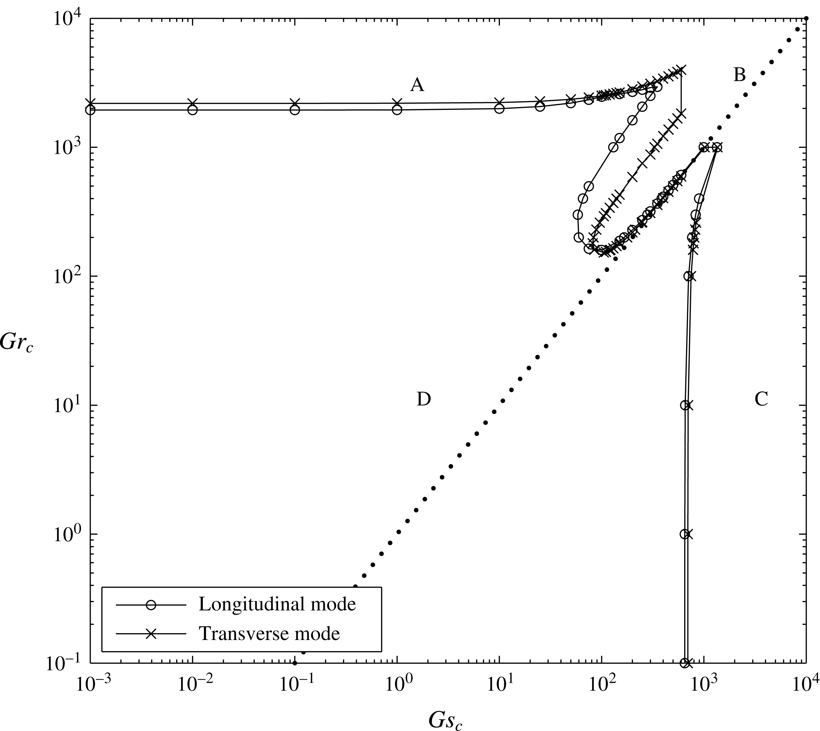
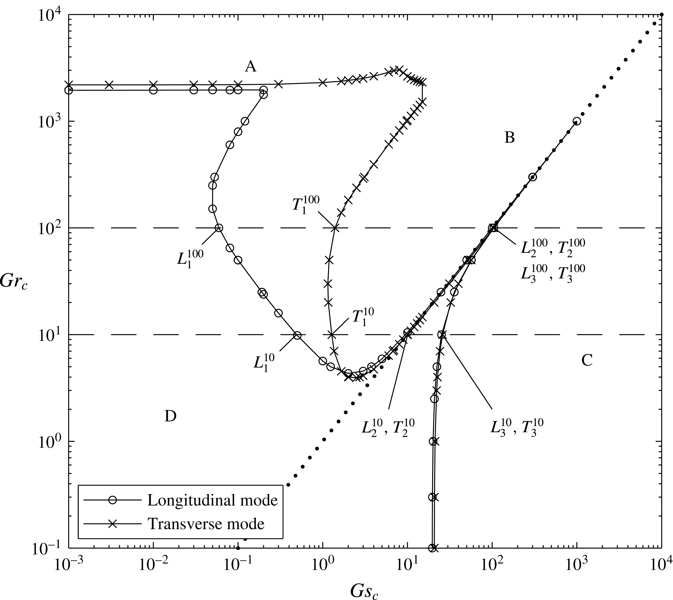
and 100 are exactly the same as those of Chan et al. (Reference Chan, Chen and Chen2002) because the formulations of both studies are identical. But the results of the transverse mode of the present study are significantly different from those of Chan et al. (Reference Chan, Chen and Chen2002). For both the longitudinal and transverse modes, the stability boundaries separate the stability map into four regions of different stability characteristics: the thermal-diffusive regime denoted with A, the salt-finger regime with B, the solute-diffusive regime with C and the stable regime with D, as shown in figures 2 and 3.
4.1 The case
$Le=3$

Figure 2 illustrates the stability boundaries of the
 $Le=3$
case in terms of
 $Gr_{c}$
and
 $Gs_{c}$
. The stability boundaries of the transverse and longitudinal modes are very close for the thermal-diffusive regime A and the solute-diffusive regime C, while there is a larger difference for the salt-finger regime B lying within
 $Gr_{c}>100$
and
 $Gs_{c}>50$
. In the regime B, the complex eigenvalues are
 $\unicode[STIX]{x1D70E}_{r}>0$
and
 $\unicode[STIX]{x1D70E}_{i}=0$
, implying that the onset of instability is a steady salt-finger mode occurring in the central portion of the convecting layer, having a wavelength approximately the height of the convecting layer (see figure 9 of Chan et al.
Reference Chan, Chen and Chen2002). This can be rationalized by examining the basic state of (2.7)–(2.9) (or the central portion of figure 6 of Chan et al.
Reference Chan, Chen and Chen2002) showing that the solute gradient is destabilizing the flow and the temperature gradient is stabilizing, which is conducive to a salt-finger instability. Consequently, regime B lies above the straight line
 $Gr_{c}=Gs_{c}$
holding invariably the relation
 $Gr_{c}>Gs_{c}$
. As
 $Gr_{c}$
is fixed, the longitudinal mode has a smaller
 $Gs_{c}$
implying that the salt-finger instability takes the form of a longitudinal mode. This appears as a row of counter-rotating vortices in the longitudinal plane, as observed in the experiments of Chen & Chen (Reference Chen and Chen1997) and Chan et al. (Reference Chan, Chen and Chen2002). As
 $Gs_{c}$
is fixed, on the other hand, the
 $Gr_{c}$
of the transverse mode is slightly lower than that of the longitudinal mode, implying that, in such a circumstance, the salt-finger instability takes the form of a transverse mode. Nevertheless, in view of the fact that the area of regime B of the longitudinal mode is larger than that of the transverse mode, the possibility of the occurrence of the longitudinal mode is generally higher.
The stability boundaries of the transverse and longitudinal modes for
 $Le=3$
. Letter A denotes the thermal-diffusive regime, B the salt-finger regime, C the solute-diffusive regime and D the stability regime. The dotted line shows
 $Gr_{c}=Gs_{c}$
.

The stability boundaries of the transverse and longitudinal modes for
 $Le=100$
. Letter A denotes the thermal-diffusive regime, B the salt-finger regime, C the solute-diffusive regime and D the stability regime. Two dashed lines at
 $Gr_{c}=10$
and
 $Gr_{c}=100$
are the two cases considered in the three-dimensional analyses. On each dashed line, there are six points corresponding to the extreme values of the neutral curves shown on figures 4 and 5. The dotted line shows
 $Gr_{c}=Gs_{c}$
.

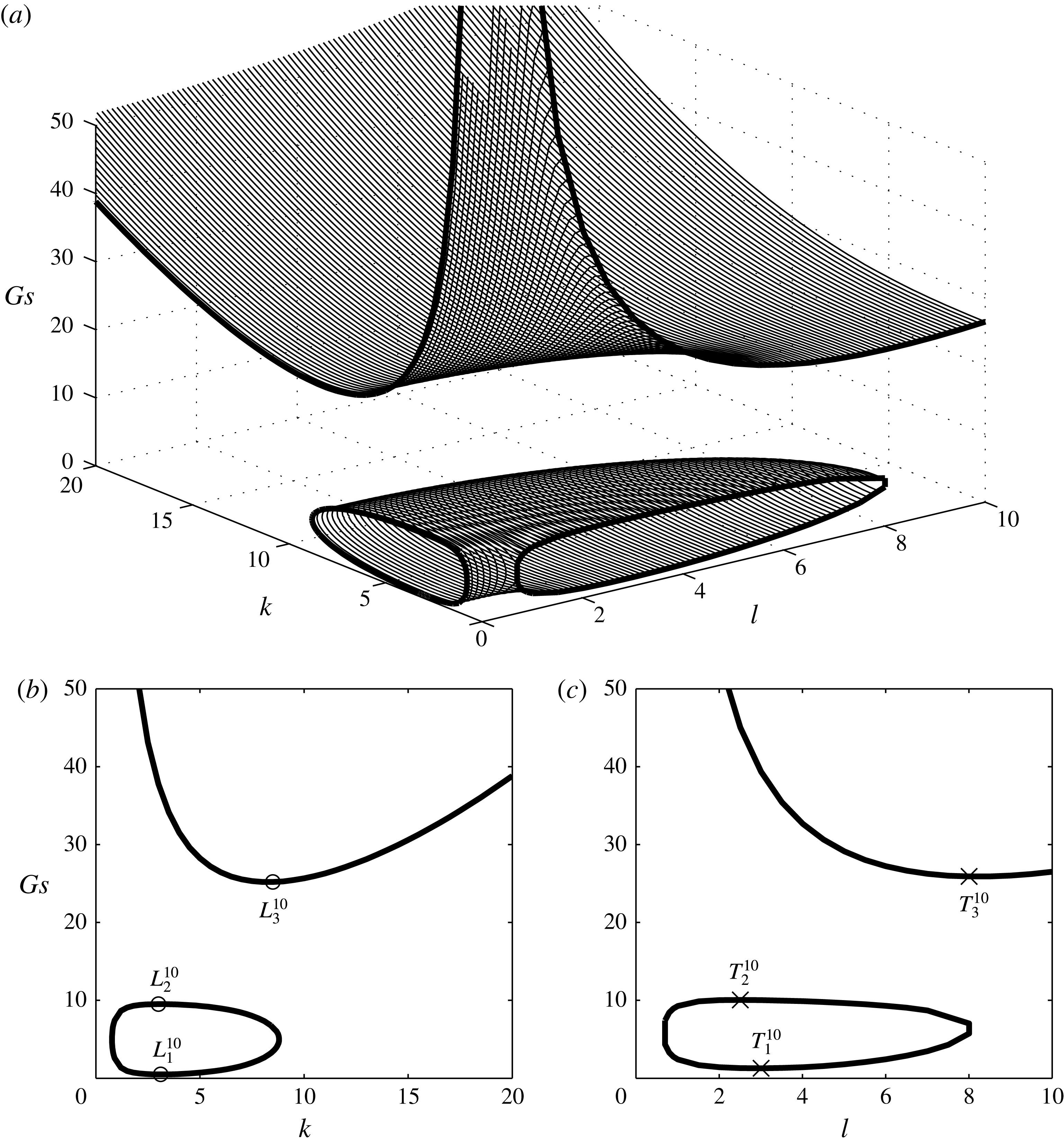
(a) The neutral surfaces of
 $Gr_{c}=10$
and
 $Le=100$
, a combination of 101 neutral curves in the
 $Gs$
–
 $k$
plane. (b) The neutral curves in the
 $Gs$
–
 $k$
plane for the longitudinal mode, for which
 $L_{1}^{10}$
,
 $L_{2}^{10}$
and
 $L_{3}^{10}$
denote the extreme values of the curves. (c) The neutral curves in the
 $Gs$
–
 $l$
plane for the transverse mode, for which
 $T_{1}^{10}$
,
 $T_{2}^{10}$
and
 $T_{3}^{10}$
denote the extreme values of the curves.

(a) The neutral surfaces of
 $Gr_{c}=100$
and
 $Le=100$
, a combination of 101 neutral curves in the
 $Gs$
–
 $k$
plane. (b) The neutral curves in the
 $Gs$
–
 $k$
plane for the longitudinal mode, for which
 $L_{1}^{100}$
,
 $L_{2}^{100}$
and
 $L_{3}^{100}$
denote the extreme values of the curves. (c) The neutral curves in the
 $Gs$
–
 $l$
plane for the transverse mode, for which
 $T_{1}^{100}$
,
 $T_{2}^{100}$
and
 $T_{3}^{100}$
denote the extreme values of the curves.

In the thermal-diffusive regime A which lies in
 $0\leqslant Gs_{c}<10$
, the flow becomes unstable as the temperature gradient (accounted for by
 $Gr$
) increases beyond the critical value, which, as shown in figure 2, is 1941.45 for the longitudinal mode and 2218.91 for the transverse mode. The
 $Gr_{c}$
for the longitudinal mode is exactly the same as predicted by Chan et al. (Reference Chan, Chen and Chen2002), while that of the transverse mode is much lower than the predicted value of approximately 8000 by Chan et al. (Reference Chan, Chen and Chen2002). This is obviously a consequence of the missed
 $Gr$
and
 $Le$
and a wrong term in their equations for the transverse mode. As
 $Gs_{c}>0$
, the purely thermal-diffusive case gradually becomes the double-diffusive case, the
 $Gr_{c}$
values of the two modes remain virtually the same with increasing
 $Gs_{c}$
, suggesting that the solute gradient is so small that the stability characteristics of the two modes are hardly influenced by the presence of the solute gradient. In such a circumstance, the onset of instability occurs in the shallow regions near the upper and lower boundaries of the convecting layer where the temperature gradient predominates the instability, having a wavelength approximately half the height of the convecting layer, see figure 10 of Chan et al. (Reference Chan, Chen and Chen2002).
In the solute-diffusive regime C, which lies below the straight line
 $Gr_{c}=Gs_{c}$
or more precisely in the region
 $Gs_{c}>600$
for the present case, the complex eigenvalues are
 $\unicode[STIX]{x1D70E}_{r}>0$
and
 $\unicode[STIX]{x1D70E}_{i}>0$
, implying that the onset of instability is oscillatory. The solute gradient serves to destabilize the flow while the temperature gradient is stabilizing. The onset of instability is largely confined to the shallow regions near the upper and lower boundaries of the convecting layer, similar to the thermal-diffusive regime A. For the purely solute-driven case
 $Gr_{c}\approx 0$
, the critical
 $Gs$
values for the longitudinal and the transverse modes respectively are 650.29 and 698.28. As
 $Gr_{c}>0$
, the purely solute-driven case turns gradually into the double-diffusive case, the critical
 $Gs$
values of the two modes remain virtually the same when
 $Gr_{c}<100$
, suggesting that the temperature gradient is too small to influence the stability characteristics of the two modes. On the other hand, the fact that the stability boundaries of the two modes are nearly overlapped suggests that the presence of temperature gradient leads to a suppression of the stability difference between the two modes.
It is interesting to note that, for the thermal-diffusive case of regime A, the
 $Gr_{c}$
values of both the longitudinal and transverse modes approach constants which are of relatively small difference. This is because, as explained previously, the solute gradient is too small to differentiate the stability characteristics of the two modes. A similar situation applies to the solute-diffusive case of regime C in which the
 $Gs_{c}$
values of both modes also approach constants of very small difference. For
 $Gr_{c}>100$
and
 $Gs_{c}>100$
, the critical conditions of both modes approach asymptotically the identity
 $Gr_{c}=Gs_{c}$
, implying that the solute and thermal gradients play an equally important role in the determination of the stability characteristics and the longitudinal and transverse modes may occur in the same condition. Consequently, no preference direction is taken by the convection and the onset of convection may occur as a hexagonal cell instead of a two-dimensional roll such as with the longitudinal mode or the transverse mode.
4.2 The case
$Le=100$

For the case
 $Le=100$
, which is the case of the salt-water solution used in the experiments of Chen & Chen (Reference Chen and Chen1997) and Chan et al. (Reference Chan, Chen and Chen2002), the stability boundaries of the longitudinal and transverse modes are shown in figure 3. It is seen that the stability boundaries of the two modes are very close in both regimes A (or
 $Gs_{c}<0.07$
, very small
 $Gs$
) and C (or
 $Gs_{c}>20$
), while the longitudinal mode is always slightly more unstable. For the purely thermal-driven case
 $Gs_{c}=0$
, the critical
 $Gr$
is 1947.26 for the longitudinal mode and 2190.42 for the transverse mode, which are very close to those of
 $Le=3$
. For the purely solute-driven case
 $Gr_{c}\approx 0$
, the critical
 $Gs$
is 19.61 for the longitudinal mode and 20.75 for the transverse mode, which are much smaller than the those for
 $Le=3$
.
In the salt-finger regime B, like the case
 $Le=3$
, the area of the unstable region of the longitudinal mode is much larger than that of the transverse mode, suggesting that the onset of the salt-finger instability has a higher possibility of taking the form of a longitudinal mode. Regime B is separated from regime C by the line
 $Gr_{c}=Gs_{c}$
. The onset of instability occurs as a solute-diffusive mode when
 $Gr_{c}<Gs_{c}$
and is salt-finger mode when
 $Gr_{c}>Gs_{c}$
. When compared with
 $Le=3$
, the area of regime B of the two modes is much larger and so is the difference between their stability boundaries. Physically, this means that a larger thermal diffusivity (or a larger
 $Le$
) makes the temperature gradient less powerful in affecting the instability while the solute gradient in turn plays a more important role. As a result, it takes a smaller
 $Gs_{c}$
to trigger the instability so that, for example, the onset of salt-finger instability occurs at
 $Gs_{c}>0.05$
for
 $Le=100$
, compared with
 $Gs_{c}>60$
for
 $Le=3$
. Generally, for a case of larger
 $Le$
, both
 $Gs_{c}$
and
 $Gr_{c}$
are smaller than a case of smaller
 $Le$
. On a whole, in both
 $Le=3$
and 100, the longitudinal mode is constantly more unstable than the transverse mode.
5 Results from three-dimensional analysis
In the three-dimensional stability analysis, we consider
 $Le=100$
and focus on the two cases
 $Gr_{c}=10$
and 100. The reason for this is because, firstly,
 $Le=100$
stands for the salt-water solution system considered by most experimental investigations, and secondly,
 $Gr_{c}=10$
and 100 are the two cases can cover (i) regime B, the longitudinal mode is unstable, the transverse mode is stable; (ii) regime B, both the longitudinal and transverse modes are unstable; (iii) regime C, both the longitudinal and transverse modes are unstable. On the other hand, the reason we did not choose the case of
 $Gr_{c}=3000$
(regime A) is because it does not cross any stability boundary and its result may not be able to reveal sufficient information about the stability characteristics in the three-dimensional domain.
For the first case
 $Gr_{c}=10$
and
 $Le=100$
, the results are shown in figure 4. We search for the neutral curves in the longitudinal plane (or
 $Gs$
–
 $k$
plane) for each value of
 $l$
, which increases from 0 to 10 by an increment of
 $\unicode[STIX]{x0394}l=0.1$
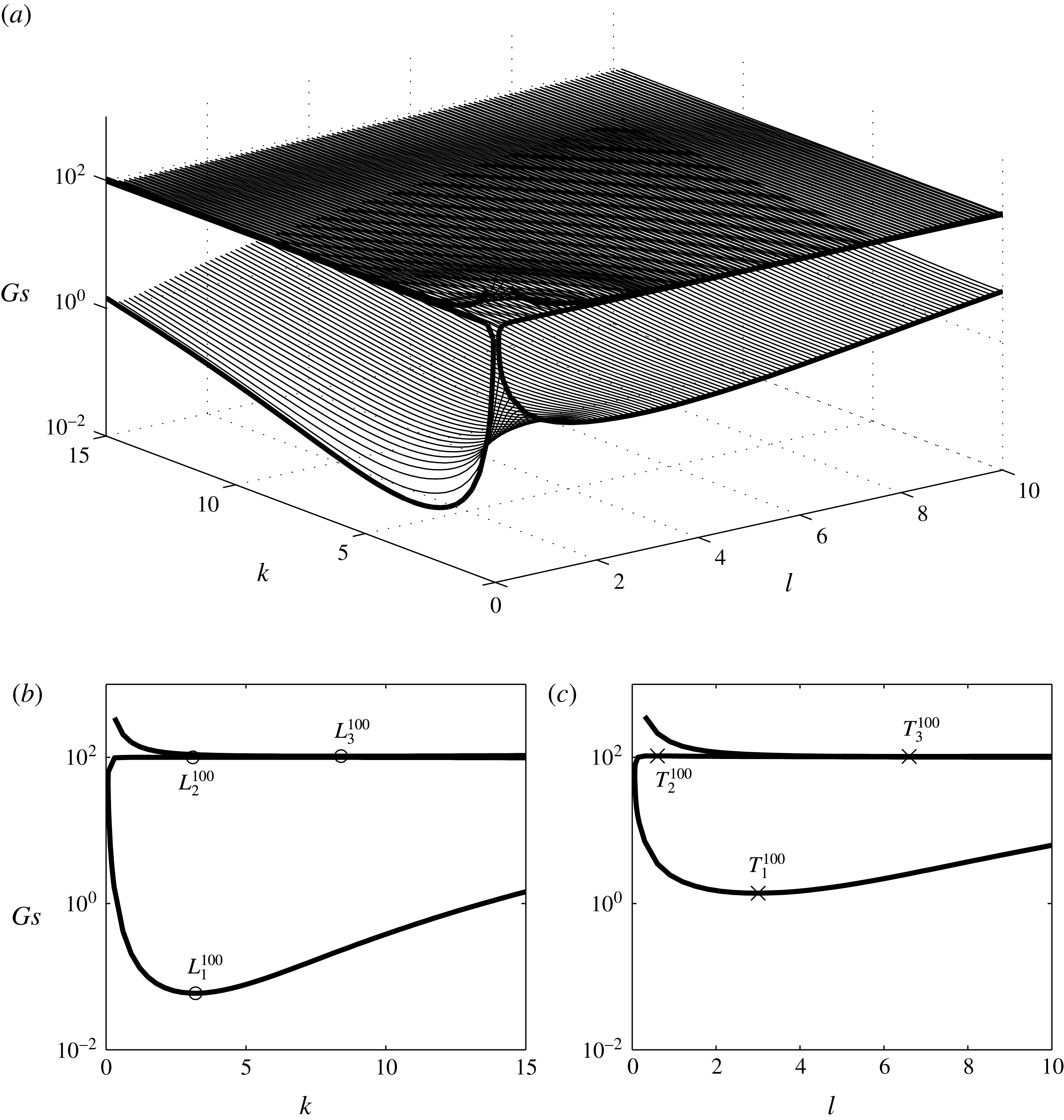
. There are a total of 101 sets of neutral curves shown in figure 4(a), and the neutral curves for longitudinal mode are shown in figure 4(b) and those for the transverse mode in figure 4(c). It is seen from figure 4(a) that there are two neutral surfaces, the upper surface in an open-valley shape accounts for the oscillatory solute-diffusive mode and the lower surface in a quarter-donut shape accounts for the steady salt-finger mode. A careful examination of the numerical data of these two surfaces concludes that the lowest values of both neutral surfaces lie in the
 $Gs$
–
 $k$
plane, indicating that the longitudinal mode is the most unstable mode in the present case. This can be seen more clearly by comparing the neutral curves in the
 $Gs$
–
 $k$
plane in figure 4(b) and the
 $Gs$
–
 $l$
plane in figure 4(c) which shows that the lowest
 $Gs$
of the longitudinal mode, denoted by
 $L_{1}^{10}$
, is obviously smaller than the lowest
 $Gs$
, denoted by
 $T_{1}^{10}$
, of the transverse mode.
Also shown in figure 4(b) are the cases denoted by
 $L_{1}^{10}$
,
 $L_{2}^{10}$
and
 $L_{3}^{10}$
for the longitudinal mode. The first two points are respectively the local minimum and maximum of the salt-finger mode and the third point is the local minimum of the solute-diffusive mode. We also show these three points in figure 3, from which one may understand the way to build up the stability boundary of the longitudinal mode, which is composed of the local minimum and maximum of the neutral curves. Similarly, in figure 4(c) the local minimum and maximum of the salt-finger mode, denoted respectively by
 $T_{1}^{10}$
and
 $T_{2}^{10}$
, and the local minimum of solute-diffusive mode, denoted by
 $T_{3}^{10}$
, are shown, which are also shown in figure 3. By examining the relation between figures 3 and 4(b), one can find that the
 $Gs$
values of
 $L_{1}^{10}$
and
 $T_{1}^{10}$
are of significant difference while the differences between
 $L_{1}^{10}$
and
 $T_{2}^{10}$
and between
 $L_{3}^{10}$
and
 $T_{3}^{10}$
are very small.
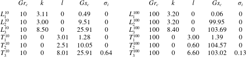
The relevant eigenvalues of these six points are shown in table 1 to illustrate their stability characteristics. For the salt-finger modes accounted for by the four points
 $L_{1}^{10}$
,
 $L_{2}^{10}$
,
 $T_{1}^{10}$
and
 $T_{2}^{10}$
on the stability boundaries, they have invariably
 $\unicode[STIX]{x1D70E}_{i}=0$
corresponding to the steady mode and have a wavenumber lying between 2.5 and 3.2, equivalent to a wavelength approximately the height of convecting layer. For the two points
 $L_{3}^{10}$
and
 $T_{3}^{10}$
, the corresponding wavenumbers are respectively 8.5 and 8.0, implying that the onset of the solute-diffusive mode lies within the shallow region near the boundary between the convecting layers. The case
 $T_{3}^{10}$
has
 $\unicode[STIX]{x1D70E}_{i}=0.64$
corresponding to an oscillatory solute-diffusive mode;
 $L_{3}^{10}$
has
 $\unicode[STIX]{x1D70E}_{i}=0$
corresponding to a steady solute-diffusive mode. By examining the values of
 $Gs_{c}$
, it is realized that the longitudinal mode denoted by
 $L_{1}^{10}$
is the most unstable one when compared with the other five points.
Relevant eigenvalues for the 12 points shown in figure 3. Since these points sit right on the stability boundaries, their
 $\unicode[STIX]{x1D70E}_{r}$
values are invariably zero.

For the second case considered, which is
 $Gr_{c}=100$
and
 $Le=100$
, the neutral surfaces shown in figure 5(a) are again composed of the upper surface accounting for the solute-diffusive mode and the lower surface accounting for the salt-finger mode. The upper surface, however, is virtually a flat plane except in the small area close to the origin at
 $k=0$
and
 $l=0$
where the value of
 $Gs$
increases dramatically. The lower surface again has a quarter-donut shape with a much larger volume than for
 $Gr_{c}=10$
. The upper portion of the donut is almost a flat plane, which is virtually overlapped with the bottom of the upper surface. This virtually overlapped relation between these two neutral surfaces can be seen clearly from the neutral curves of the longitudinal mode of figure 5(b) and the transverse mode of figure 5(c). In the region near
 $Gs=100$
, the
 $Gs$
values of these two neutral curves (or the two nearly flat surfaces) are indeed very close but never the same.
Also shown in 5(b) and 5(c) are the local minimum and maximum of the salt-finger mode denoted respectively by
 $L_{1}^{100}$
and
 $L_{2}^{100}$
for the longitudinal mode and
 $T_{1}^{100}$
and
 $T_{2}^{100}$
for the transverse mode. The local minimum of the solute-diffusive curve denoted by
 $L_{3}^{100}$
for the longitudinal mode and
 $T_{3}^{100}$
for the transverse mode are also shown. By examining the relation between figures 3 and 5(b,c) and the numbers shown in table 1, it is found that the
 $Gs$
values of
 $L_{1}^{100}$
and
 $T_{1}^{100}$
are respectively 0.06 and 1.39, which are of significant difference by proportion. When the
 $Gs$
values corresponding to
 $L_{2}^{100}$
,
 $L_{3}^{100}$
,
 $T_{2}^{100}$
and
 $T_{3}^{100}$
are examined, it is seen that their values lie within the range between 100 and 105, being truly very close by proportion but never the same by value. Physically, it is inferred that the salt-finger longitudinal mode is much more unstable than the salt-finger transverse mode, while the solute-diffusive modes in both the longitudinal and transverse planes have virtually the same stability criteria. As one examines the critical wavenumbers of these six points in table 1, it is realized that the wavenumber of the transverse mode varies widely from 0.6 to 6.6, while that of the longitudinal mode generally can be categorized into two modes: a wavenumber around 3.2 corresponding to the salt-finger mode and a wavenumber around 8.4 corresponding to the solute-diffusive mode.
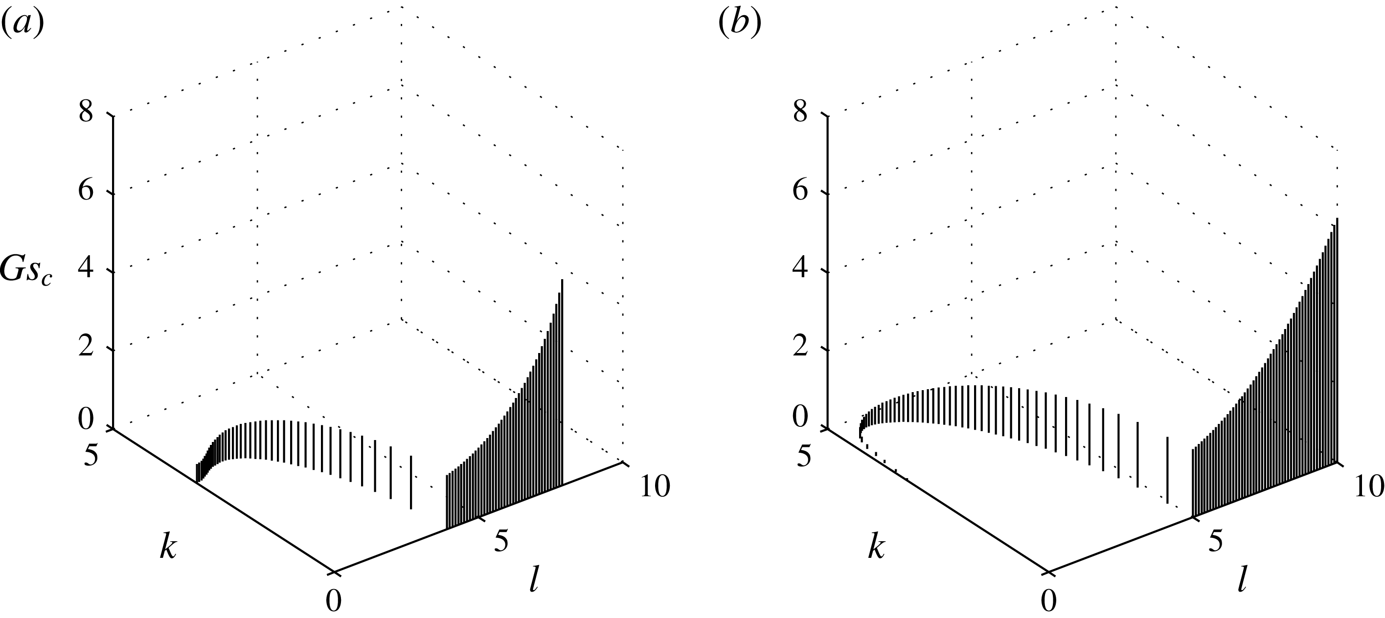
The track of
 $Gs_{c}$
values of the neutral curve in each of the 101
 $Gs$
–
 $k$
planes at different
 $l$
. (a)
 $Gr=10$
(b)
 $Gr=100$
.

We summarize the
 $Gs_{c}$
values of the neutral curves in each of the 101
 $Gs$
–
 $k$
planes at different
 $l$
in figure 6(a) for
 $Gr=10$
and in figure 6(b) for
 $Gr=100$
. For both cases, the
 $Gs_{c}$
values correspond to the salt-finger mode accounted for by the lowest points of the quarter-donut surface. For
 $Gr=10$
, the
 $Gs_{c}$
-track starts from
 $k=3.11$
,
 $l=0$
, follows a curve with increasing
 $k$
and
 $l$
and ends at
 $k=0$
,
 $l=3.01$
. After that, the
 $Gs_{c}$
stays within the
 $Gs_{c}$
–
 $l$
plane while increasing exponentially with
 $l$
. For
 $Gr=100$
, the
 $Gs_{c}$
-track starts from
 $k=3.20$
,
 $l=0$
and ends at
 $k=0$
,
 $l=5.00$
, following a curve on which
 $l$
increases constantly while
 $k$
decreases first and increases later. For both cases
 $Gr=10$
and 100 considered, the lowest
 $Gs_{c}$
invariably lies in the
 $Gs_{c}$
–
 $k$
plane at
 $l=0$
, confirming that the longitudinal mode is generally the most unstable. Away from the
 $Gs_{c}$
–
 $k$
plane at
 $l=0$
, the value of
 $Gs_{c}$
increases with
 $k$
and
 $l$
until it reaches the
 $Gs_{c}$
–
 $l$
plane at
 $k=0$
, where the
 $Gs_{c}$
increases exponentially with
 $l$
. By comparing the two tracks of
 $Gr=10$
and 100, it is seen that the
 $Gs_{c}$
of the longitudinal mode for
 $Gr=100$
is 0.06, which is significantly lower than 0.49 of
 $Gr=10$
. Namely, the longitudinal mode is more unstable with a larger
 $Gr$
. As far as the transverse mode is concerned, the
 $Gs_{c}$
of
 $Gr=100$
is 1.39, which is slightly higher than the 1.28 of
 $Gr=10$
; i.e. the transverse mode is slightly less stable with a smaller
 $Gr$
.
6 Discussion and conclusion
We have implemented a three-dimensional stability analysis to investigate the onset of secondary instability in the convecting layer, which can be generated by imposing a horizontal temperature gradient upon a stably stratified fluid. Results indicate that two-dimensional stability analyses for the longitudinal and transverse modes separately are sufficient to predict the secondary stability of the convecting layer because the most unstable mode constantly occurs with an axis perpendicular to the longitudinal plane. For the cases
 $Le=3$
and 100 considered, the longitudinal mode was found to be the most unstable. Specifically, in both the thermal-diffusive regime A and the solute-diffusive regime C, the stability boundaries of the two modes are very close and sometimes are virtually overlapping while the longitudinal mode is invariably slightly more unstable. In the salt-finger regime B, the stability boundaries of the two modes are of significant difference and the area of the unstable region of the longitudinal mode is much larger than that of the transverse mode. On a whole, the longitudinal mode generally has a smaller
 $Gr_{c}$
or
 $Gs_{c}$
, indicating that the longitudinal mode is the most unstable mode of the convecting layer considered.
Regarding the correctness of the present results, we check the
 $Gs_{c}$
for the purely solute-driven case
 $Gr=10$
and the
 $Gr_{c}$
for the purely thermal-driven case
 $Gs=0$
. As shown in figure 2 for
 $Le=3$
, the
 $Gs_{c}$
values are 650.29 and 698.28 and the
 $Gr_{c}$
values are 1941.45 and 2218.91 for the longitudinal and transverse modes respectively. The relations between these critical values of both modes are in good agreement with the theoretical identity
 $Gs_{c}=Gr_{c}/Le$
, which helps confirm the correctness of the present results. The same conclusion can be reached for
 $Le=100$
in figure 3, where the
 $Gs_{c}$
values are 19.61 and 20.75 and the
 $Gr_{c}$
values are 1947.26 and 2190.42 for the longitudinal and transverse modes respectively. These values, again, follow closely the theoretical identity.
In comparison with the studies for thermal convection problem, we realize that Hart (Reference Hart1972) conducted a linear stability analysis for the purely thermal-driven case (or
 $Gs_{c}=0$
) and obtained
 $Gr_{c}$
values for the longitudinal and transverse mode that were respectively approximately 2100 and 1400 when
 $Pr=7$
was considered. These two values are quite different from the present results with
 $Gr_{c}$
values for purely thermal-driven case at 1941.45 (longitudinal) and 2218.91 (transverse) for
 $Le=3$
and 1947.26 (longitudinal) and 2190.42 (transverse) for
 $Le=100$
. More seriously, their results indicate that the transverse mode is invariably more unstable, which is the opposite result to the present study which finds that the longitudinal mode is more unstable, although the stability boundaries of the two modes are close. The results of Hart (Reference Hart1972) suggest that the existence of a solute gradient may not only change the value of
 $Gr_{c}$
but also switch the critical mode from the transverse mode of the thermal-diffusion system into the longitudinal mode of the present double-diffusion system. Later, Kuo et al. (Reference Kuo, Korpela, Chait and Marcus1986) conducted another study on the purely thermal-driven case and found that the transverse mode dominates for the fluid of
 $Pr<0.45$
while the longitudinal mode prevails for the fluid of
 $Pr>0.45$
, which is consistent with the results of the present study where
 $Pr=7$
is considered.
Results shown in figures 2 and 3 indicate that the stability boundaries of the longitudinal and transverse modes are very close in regimes A and C, which is in agreement with Kerr (Reference Kerr2000) who concluded the stability of the two modes are slightly different because the shear of the convection cell plays an insignificant role in the onset of the secondary instability. This implication holds true, according to the present results, only for regimes A and C. For regime B, nevertheless, the present results show that the stability boundaries of the two modes are significantly different and the longitudinal mode is generally more unstable than the transverse mode. This can be a result of the influence of shear because the longitudinal mode moves in the direction of basic convective flow and its instability can be enhanced by the shear. However the influence of shear cannot possibly induce a Rayleigh–Taylor instability because, firstly, the existence of temperature and solute gradients make the double-diffusive instability predominate in the system and suppresses the occurrence of Rayleigh–Taylor instability (Chen & Chen Reference Chen and Chen1997; Kerr Reference Kerr2000), and secondly, Rayleigh–Taylor instability leads to a transverse mode, instead of the longitudinal mode mainly occurring in the present system.
Results of figures 2 and 3 may help identify the experimental conditions under which the onset of longitudinal and transverse modes can be clearly discerned by experiment. More specifically, because the stability boundaries of the two modes in both regimes A and C virtually overlap, an experimental condition that lies in these two regimes may not lead to a situation in which the difference between the two modes can be clearly identified. The only possibility of distinguishing these two modes is to conduct an experiment with conditions lying in a region of regime B where the longitudinal mode is unstable and the transverse mode is stable or vice versa. But this is easier said than done. For example, the experiments conducted by Chen & Chen (Reference Chen and Chen1997) and Chan et al. (Reference Chan, Chen and Chen2002) were carried out under conditions lying well beyond the stability boundaries and well into a nonlinear regime. Chan et al. (Reference Chan, Chen and Chen2002, p. 10, p. 14) conducted experiments with
 $Gr=1021$
and
 $Gs=603$
, which lie in the salt-finger regime B of figure 3 (
 $Le=100$
) and well above the stability boundaries of the two modes. They concluded that only the longitudinal mode was observed while nothing was detected in the transverse plane, reflecting the difficulty of either conducting experiments under conditions close to stability boundaries or of discerning the two modes by experimental observations.
On the other hand, nevertheless, the transverse mode had been observed by Chen & Chen (Reference Chen and Chen1997) although it was not clearly identified. They conducted experiments with conditions similar to those of Chan et al. (Reference Chan, Chen and Chen2002) and applied the horizontal temperature difference either impulsively or gradually. As stated in the introduction, regardless the way the temperature difference is applied, as long as the temperature difference increases beyond the critical value, a series of convective vortices are generated consecutively. These vortices behave like a transverse mode because their axes are perpendicular to the transverse plane and their wavelengths are approximately the height of the convecting layer. Within the vortices, simultaneously, a row of counter-rotating salt-finger rolls (commonly recognized to be a longitudinal mode) occurs with their axes perpendicular to the longitudinal plane. In brief, for most of the experiments of Chen & Chen (Reference Chen and Chen1997), both the transverse and longitudinal modes occur virtually simultaneously with the formation of the convecting layer. This fact may reveal the value of the present results as follows. Although the longitudinal mode is found to be always more unstable than the transverse mode, as shown in figure 4, the
 $Gs_{c}$
values of these two mode are only slightly different, implying that in the weakly nonlinear or nonlinear regime, under some circumstances, the transverse mode may prevail. The results of figure 4, accordingly, may help researchers to select cases preferred for nonlinear study.
Strictly speaking, the experimental conditions of Chan et al. (Reference Chan, Chen and Chen2002) and Chen & Chen (Reference Chen and Chen1997) were well beyond the linear stability boundaries and fell into the nonlinear regime. To examine the stability characteristics of these flows, a fully nonlinear stability analysis or a weakly nonlinear stability analysis shall be performed. The present linear stability analysis can only offer a suggestion to explain the physical characteristics of these nonlinear flows, and should not be seen as the solution equivalent to the experimental findings. On the other hand, however, it is still reasonable to conjecture that these nonlinear phenomena can be an extension of the linear regime. Under some circumstances, in general, the onset of instability from small perturbations may preserve the stability characteristics in terms of the wavelength and the direction of motion well into the nonlinear regime, which may happen in the present case. However, after all, a careful treatment of nonlinearity of the convecting layer can surely help inform the connection between the linear and nonlinear regimes.