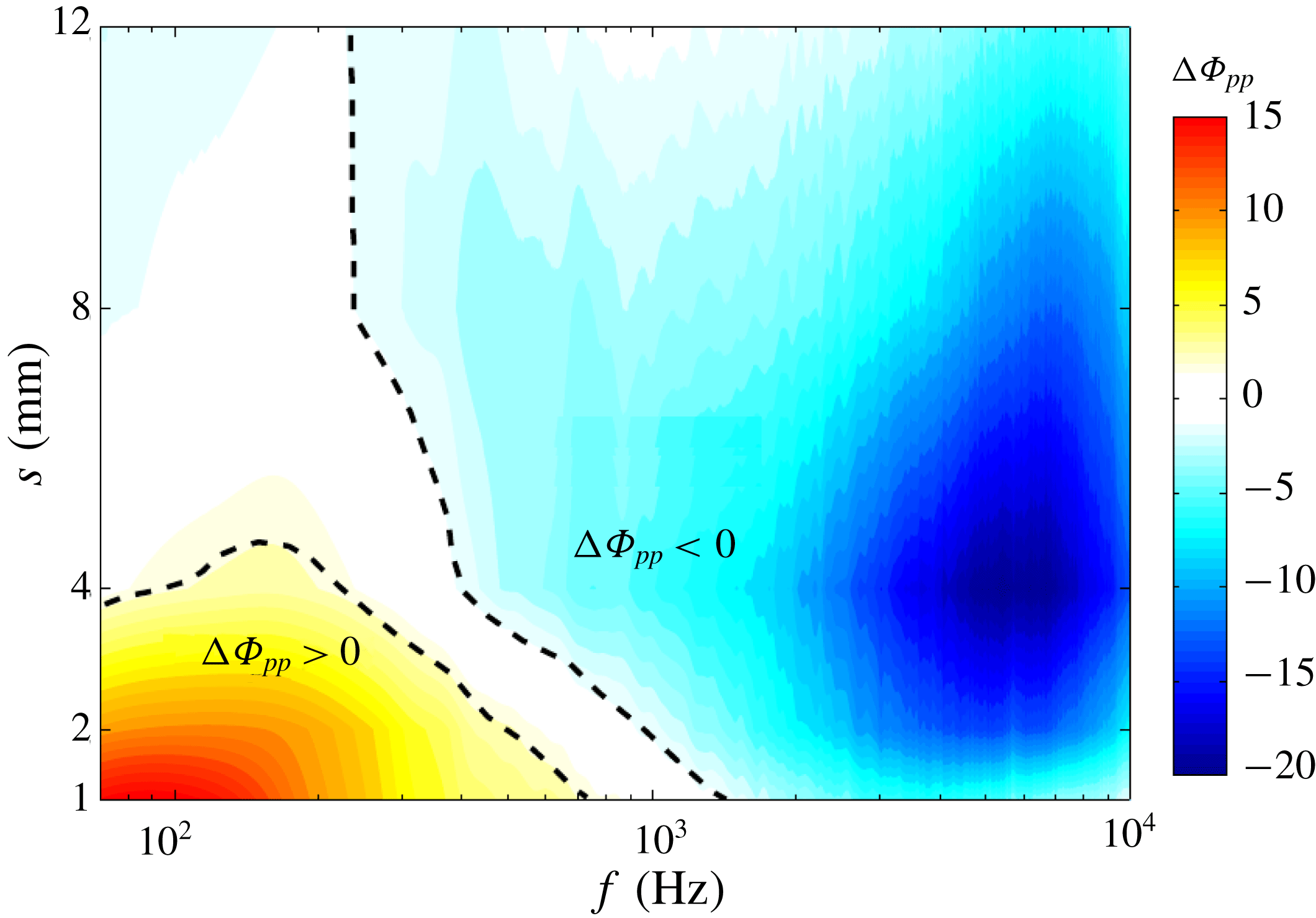
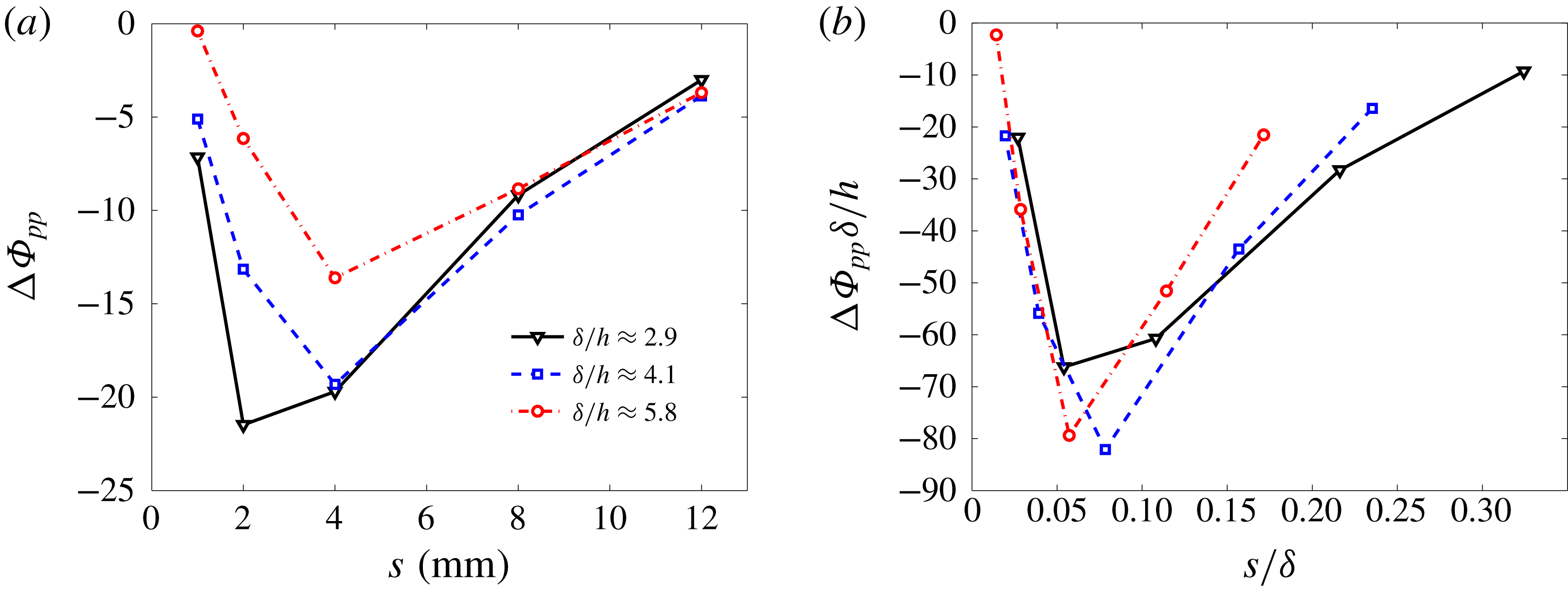
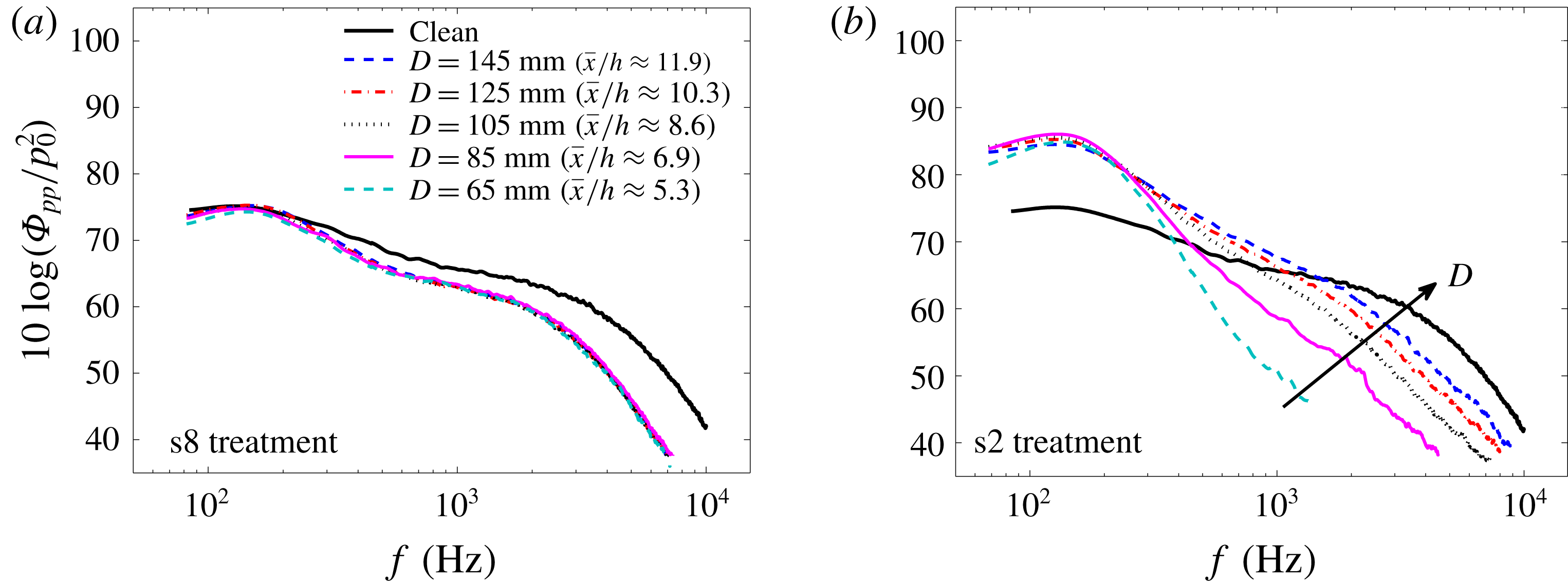
1 Introduction
Airfoil self-noise is generated when the airfoil interacts with its own boundary layer and near wake. There are a number of specific noise-generating components associated with airfoil self-noise that are concisely summarized by Brooks, Pope & Marcolini (Reference Brooks, Pope and Marcolini1989). Turbulent boundary layer trailing-edge noise is one of the most important and commonly encountered types of aerodynamically generated noise. Trailing-edge noise is categorized as an edge noise and is considered as the dominant noise source in various engineering applications, such as wind turbine noise, airframe noise, fan noise, etc. (Brooks et al. Reference Brooks, Pope and Marcolini1989). The physical process of trailing-edge noise has previously been described by Amiet (Reference Amiet1976) and Roger & Moreau (Reference Roger and Moreau2004). Over recent decades, trailing-edge noise and its suppression at source have received considerable research attention in the form of theoretical, computational and experimental activities (Ffowcs Williams & Hall Reference Ffowcs Williams and Hall1970; Howe Reference Howe1978; Brooks & Hodgson Reference Brooks and Hodgson1981; Blake Reference Blake2017).
Numerous theoretical models have been developed for the prediction of the trailing-edge noise over the past decades, as summarized by Roger & Moreau (Reference Roger and Moreau2004) and Lyu, Azarpeyvand & Sinayoko (Reference Lyu, Azarpeyvand and Sinayoko2016). Formulations based on linearized hydroacoustic methods are one of the basic approaches for the prediction of the far-field trailing-edge noise, which rely on the induced hydrodynamic pressure field at some distance upstream of the trailing edge. The majority of trailing-edge noise prediction models have been formulated based on the surface pressure fluctuations, as unsteady surface pressure measurements can be easily made using flush-mounted pressure transducers. According to the formulations of Amiet (Reference Amiet1976) and Howe (Reference Howe1978), the wall pressure point spectrum and the frequency-dependent spanwise length scale of the surface pressure fluctuations are the crucial quantities in the determination of the far-field trailing-edge noise. While the point spectrum defines the strength of the turbulent structures passing over the trailing edge as a function of frequency, the spanwise correlation length describes the extent of the boundary layer eddies along the span of the trailing edge. One can therefore conclude that reducing the wall pressure spectrum level and/or the spanwise turbulent length scale in the trailing-edge region can result in the reduction of the trailing-edge noise.
To reduce the turbulent boundary layer trailing-edge noise, various passive airfoil noise-control methods have been developed, such as trailing-edge serrations (Howe Reference Howe1991; Dassen et al. Reference Dassen, Parchen, Bruggeman and Hagg1996; Oerlemans et al. Reference Oerlemans, Fisher, Maeder and Kögler2009; Lyu et al. Reference Lyu, Azarpeyvand and Sinayoko2016; Liu et al. Reference Liu, Kamliya Jawahar, Azarpeyvand and Theunissen2017), trailing-edge brushes (Herr & Dobrzynski Reference Herr and Dobrzynski2005; Finez et al. Reference Finez, Jondeau, Roger and Jacob2010), porous trailing edge (Howe Reference Howe1979; Geyer, Sarradj & Fritzsche Reference Geyer, Sarradj and Fritzsche2010; Ali et al. Reference Ali, Azarpeyvand, Szőke and Ilário da Silva2018a ; Ali, Azarpeyvand & Ilário da Silva Reference Ali, Azarpeyvand and Ilário da Silva2018b ), airfoil shape optimization (Jones, Crossley & Lyrintzis Reference Jones, Crossley and Lyrintzis2000; Oerlemans et al. Reference Oerlemans, Fisher, Maeder and Kögler2009), trailing-edge morphing (Ai et al. Reference Ai, Azarpeyvand, Lachenal and Weaver2016; Jawahar, Ai & Azarpeyvand Reference Jawahar, Ai and Azarpeyvand2018) and recently upstream surface treatment (Clark et al. Reference Clark, Alexander, Devenport, Glegg, Jaworski, Daily and Peake2017), which is inspired by the anatomy of silently flying owls. It was shown both analytically (Howe Reference Howe1991; Lyu et al. Reference Lyu, Azarpeyvand and Sinayoko2016) and experimentally (Dassen et al. Reference Dassen, Parchen, Bruggeman and Hagg1996; Oerlemans et al. Reference Oerlemans, Fisher, Maeder and Kögler2009) that trailing-edge noise level can be reduced by implementing trailing-edge serration, through destructive interference of the sound field radiated from the edges of the serrations. In fact, the addition of trailing-edge serration leads to a reduction in the effective spanwise length of the trailing edge. Experimental data have also shown that misalignment of the serrations can increase the far-field noise (Dassen et al. Reference Dassen, Parchen, Bruggeman and Hagg1996). The use of flexible trailing-edge brushes has demonstrated a significant noise reduction potential in wind-tunnel tests on flat plates and on a two-dimensional (2-D) airfoil (Herr & Dobrzynski Reference Herr and Dobrzynski2005; Finez et al. Reference Finez, Jondeau, Roger and Jacob2010). Porous trailing edges can also significantly reduce the sound pressure level at low to mid-frequencies. However, an increase in noise at higher frequencies was also observed, which was attributed to surface roughness effects (Geyer et al. Reference Geyer, Sarradj and Fritzsche2010). Moreover, brush and porous edge attachments may have practical limitations; namely, the fine pores or spaces between brushes are prone to collect dirt and insects, making them ineffective. Airfoil shape optimization, such as the modification of the thickness or the trailing-edge flap curve, can significantly affect the flow field around the airfoil, leading to improvement in both the aerodynamic and aeroacoustic performance of the airfoil (Jones et al. Reference Jones, Crossley and Lyrintzis2000). Trailing-edge morphing can also effectively reduce the airfoil trailing-edge noise over a wide range of flow speeds and angles of attack (Ai et al. Reference Ai, Azarpeyvand, Lachenal and Weaver2016; Jawahar et al. Reference Jawahar, Ai and Azarpeyvand2018).
In 2016, Clark et al. (Reference Clark, Daly, Devenport, Alexander, Peake, Jaworski and Glegg2016) used a series of surface canopies, inspired by the owls’ downy coating, over rough surfaces to suppress roughness noise. All canopies were observed to have a strong influence on the wall surface pressure spectrum, and attenuations of up to 30 dB were observed. This development represented a new passive method for roughness noise control. The method was then used for reducing trailing-edge noise at source. Clark et al. (Reference Clark, Alexander, Devenport, Glegg, Jaworski, Daily and Peake2017) studied the use of different surface treatments, referred to as finlets, for reducing the trailing-edge noise for a tripped DU96-W180 airfoil. The treatments were installed directly upstream of the trailing edge to modify the boundary layer prior to interacting with the trailing edge. Compared to the untreated airfoil, the treatments were found to be effective, providing broadband trailing-edge noise attenuation of up to 10 dB. The effect of extending the treatments beyond the trailing edge is also examined by Clark et al. (Reference Clark, Alexander, Devenport, Glegg, Jaworski, Daily and Peake2017), and they concluded that the finlets reduce the trailing-edge noise by manipulating the boundary layer structures as they reach the trailing-edge area, rather than altering the scattering efficiency of the trailing edge, as is accomplished by trailing-edge serrations or combs. Furthermore, the aerodynamic impact of the treatment appeared to be minimal. However, their investigation was limited to far-field noise measurements and the physical phenomenon attributed to this novel noise-control method was not properly addressed.
The use of micro surface treatments as a means of passive flow control, in particular for drag reduction and flow laminarization, has been a topic of intensive research over the last three decades. The shape of these microstructure surface treatments, known as riblets, has been imitated from the micro surface structure of shark skin. Two-dimensional streamwise riblets have been widely studied (Bechert et al.
Reference Bechert, Bruse, Hage, Van der Hoeven and Hoppe1997; Lee & Lee Reference Lee and Lee2001; Dean & Bhushan Reference Dean and Bhushan2010) and shown to be effective in reducing the turbulent skin friction drag by as much as 10 % (Bechert et al.
Reference Bechert, Bruse, Hage, Van der Hoeven and Hoppe1997). The drag reduction results are typically presented as a function of
 $s^{+}$
, which represents the riblet spacing (
 $s$
) normalized by the wall shear velocity and the viscosity of the fluid. The results on the effects of the lateral spacing of the riblets have shown that the highest drag reduction occurs at
 $s^{+}\approx 15{-}17$
(Dean & Bhushan Reference Dean and Bhushan2010). In general, the reduction of drag using micro surface treatment has been attributed to two main mechanisms: first, riblets impede the cross-stream translation of the streamwise vortices, which causes a reduction in vortex ejection and outer layer turbulence; second, riblets lift the vortices off the surface and reduce the amount of surface area exposed to the high-velocity flow structures (Dean & Bhushan Reference Dean and Bhushan2010). However, it should be noted that, despite the geometrical similarities between the drag reduction riblet and the noise reduction finlets used in the work by Clark et al. (Reference Clark, Alexander, Devenport, Glegg, Jaworski, Daily and Peake2017) and also the current study, there also exist some differences. The drag reduction riblets are of the dimension of the boundary layer viscous sublayer, to affect the near-wall streamwise vortices, while the proposed noise-control surface treatments are larger, in order to decrease the energy content of the flow structures and likely breakup of the large coherent structures responsible for the surface pressure fluctuations at low and mid-frequencies. Given the apparent similarities between the drag reduction riblets and the aerodynamic noise-control surface treatments, one can infer that there may be an optimum finlet spacing that can lead to the highest possible reduction in the surface pressure level and/or the lateral coherence of the turbulence structures. As part of this study, we shall investigate the effects of different types of surface treatments, with different ratios of spacing to boundary layer thickness and height to boundary layer thickness, and provide experimental evidence for the underlying physics of the unsteady surface pressure reduction caused by streamwise-oriented finlets.
In the present study, the effects of upstream surface treatments (finlets), the spacing between finlets and the finlet distance from the trailing edge on the mean surface pressure distribution, the surface pressure power spectral density, the frequency-dependent spanwise length scale and the flow convection velocity in the trailing-edge region of a flat plate are investigated. It should be noted that, unlike the study of Clark et al. (Reference Clark, Alexander, Devenport, Glegg, Jaworski, Daily and Peake2017), in the present work the finlets are placed upstream of the trailing edge such that the boundary layer could be manipulated before it reaches the trailing edge. The space between the finlets and the trailing edge is also heavily instrumented so that a proper near-field study could be carried out. Furthermore, pressure–velocity coherence results will also be provided to unravel the physics of the finlet treatment flow field and the mechanisms leading to the reduction of the surface pressure fluctuations near the trailing edge. The layout of the paper is as follows. The experimental set-up and the measurement techniques used in this study are described in § 2. The results for the clean flat-plate case, i.e. no finlet treatment, are provided in § 3, which also serves as the validation of the set-up against available data in the literature. Then § 4 provides the flow-field data for different types of finlet treatments. Results will be provided for the boundary layer quantities, surface pressure fluctuations and also pressure–velocity coherence. Discussions will also be provided for the optimum finlet spacing and finlet distance from the trailing edge. Finally, § 5 concludes the paper.
2 Experimental set-up
2.1 Wind tunnel and model
The experiments were carried out in the blowdown subsonic wind tunnel of the Yazd University with a test-section size of
 $46~\text{cm}\times 46~\text{cm}$
and length of 240 cm. At the maximum speed of
 $25~\text{m}~\text{s}^{-1}$
, the free-stream turbulence intensity has been measured to be less than 0.3 %. The wall pressure fluctuation measurements are often carried out in an acoustically treated wind tunnel to avoid noise contamination due to the wind tunnel background noise. The wind tunnel used in this study has a centrifugal fan with forward-inclined blades, with low broadband and tonal noise signature. To further improve the acoustic properties of the wind tunnel, the internal solid surfaces of the wind tunnel upstream of the test section are replaced with stretched Kevlar walls, backed by a 15 cm thick porous section, similar to that of Garcia-Sagrado & Hynes (Reference Garcia-Sagrado and Hynes2012). This resulted in reduction of the background noise from the fan by up to 20 dB, making the working section suitable for this experiment.
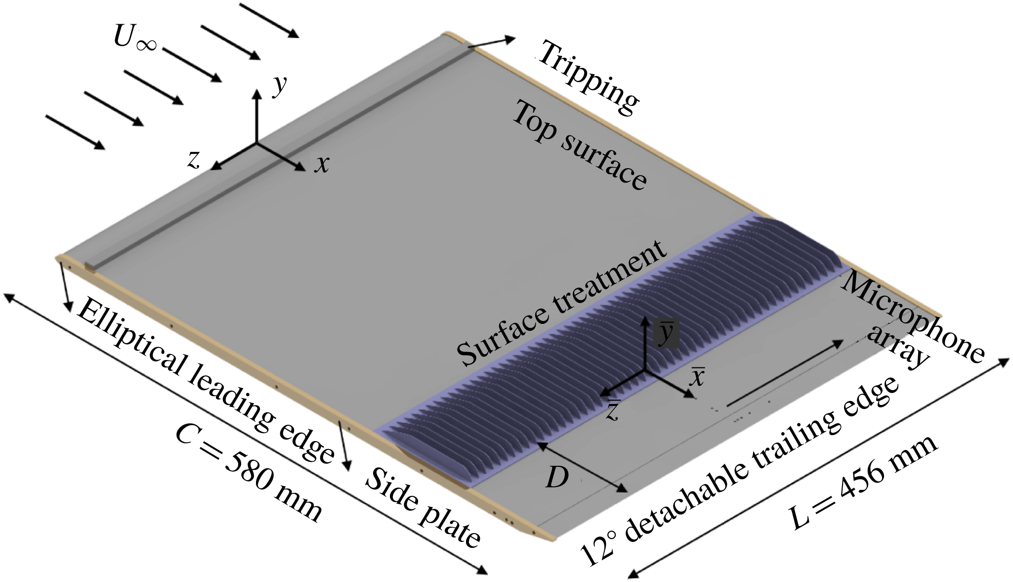
The flat plate used in the present work has a chord length of 580 mm, a span of 456 mm and a thickness of 8 mm (see figure 1). The leading edge of the model is made in an elliptical shape with a semi-major axis of 12 mm and a semi-minor axis of 4 mm. Furthermore, to realize a zero-pressure-gradient (ZPG) turbulent boundary layer on the top side, the trailing edge is asymmetrically bevelled at an angle of
 $12^{\circ }$
(Mosallem Reference Mosallem2008). The model consists of a main body and a detachable trailing-edge part, which allows the spanwise miniature microphones to be installed horizontally inside the flat-plate trailing-edge section. The trailing-edge plate is attached to the main body with two side plates. The thickness of the trailing edge is
 $t=0.4~\text{mm}$
, minimizing the possibility of trailing-edge vortex shedding generation (
 $t/\unicode[STIX]{x1D6FF}^{\ast }<0.3$
) for all free-stream velocities considered in this study (Blake Reference Blake2017). Experiments were carried out at zero angle of attack and at three different free-stream velocities,
 $U_{\infty }=10$
, 15 and
 $20~\text{m}~\text{s}^{-1}$
, corresponding to the momentum-thickness-based Reynolds numbers of
 $Re_{\unicode[STIX]{x1D703}}=3610$
, 5750 and 6840, respectively. The wind tunnel blockage ratio of the flat-plate model is less than 2 % and hence the wind tunnel wall effects on the measured quantities can be considered negligible. To ensure a fully developed turbulent boundary layer and improve the signal-to-noise ratio at low frequencies for the unsteady surface pressure measurements, the model was tripped at 5 % of the chord length downstream of the leading edge on the upper surface. The flow characteristics of the flow trip used here and comparisons against the data from the literature will be provided in § 3. The detailed computer-aided design (CAD) view of the flat-plate model is shown in figure 1. The coordinate system (
 $x,y,z$
) is placed at the leading edge of the flat plate (see figure 1). A secondary coordinate system (
 $\bar{x},\bar{y},\bar{z}$
) is also placed towards the trailing edge of the finlet treatment, as seen in figure 1, which will be used for the presentation of the results downstream of the finlets.
The flat-plate model with a detachable trailing edge and the surface treatment upstream of the trailing edge.

2.2 Instrumentation
The trailing edge of the flat-plate model is equipped with 28 static pressure ports and nine unsteady pressure transducers. The static pressure ports cover 189 mm in the streamwise direction between
 $x=384~\text{mm}$
(
 $x/c\approx 0.66$
) and
 $x=573~\text{mm}$
(
 $x/c\approx 0.99$
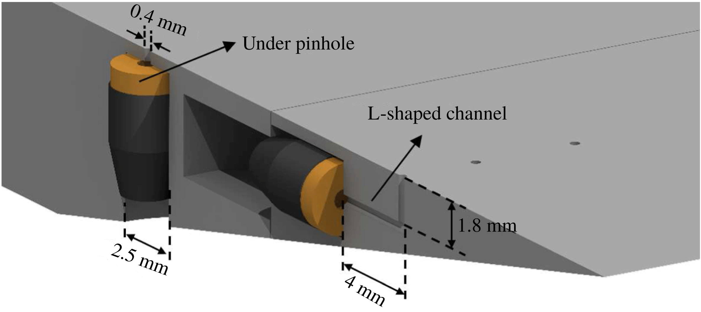
) with a spacing of 7 mm. To measure the unsteady surface pressure, miniature microphones (Knowles FG-23329-P07) are employed. The microphones are 2.5 mm in diameter, 2.5 mm in height and have a circular sensing hole diameter of 0.8 mm. The same microphones were used in other experiments (Garcia-Sagrado & Hynes Reference Garcia-Sagrado and Hynes2011; Gruber Reference Gruber2012) and have been shown to be reliable for the frequencies considered in this study. The microphones are embedded in the flat plate under a pinhole mask of 0.4 mm diameter in order to decrease the attenuation effects at high frequencies due to the finite size of the microphones sensing area. Owing to the space constraint in the trailing-edge area, two different techniques have been used for the installation of the FG microphones. For positions far from the trailing edge, the plate is thick enough to place the microphones vertically under the pinhole. For the positions near the trailing edge, the microphones have been installed inside the flat plate parallel to the surface (i.e. horizontally), linked to the pinhole via an L-shaped channel. A schematic of both arrangements is depicted in figure 2. The issue of the pinhole configuration resonant frequencies was studied analytically and experimentally, and it was demonstrated that no resonance occurs in the frequency range considered in this study (100 Hz–10 kHz). Readers interested in the calibration procedure can find the detailed process in the study of Afshari et al. (Reference Afshari, Azarpeyvand, Dehghan and Szoke2017).
Illustration of the installation of the miniature microphones: under pinhole and L-shaped channel configurations.

2.3 Layout of surface microphone array
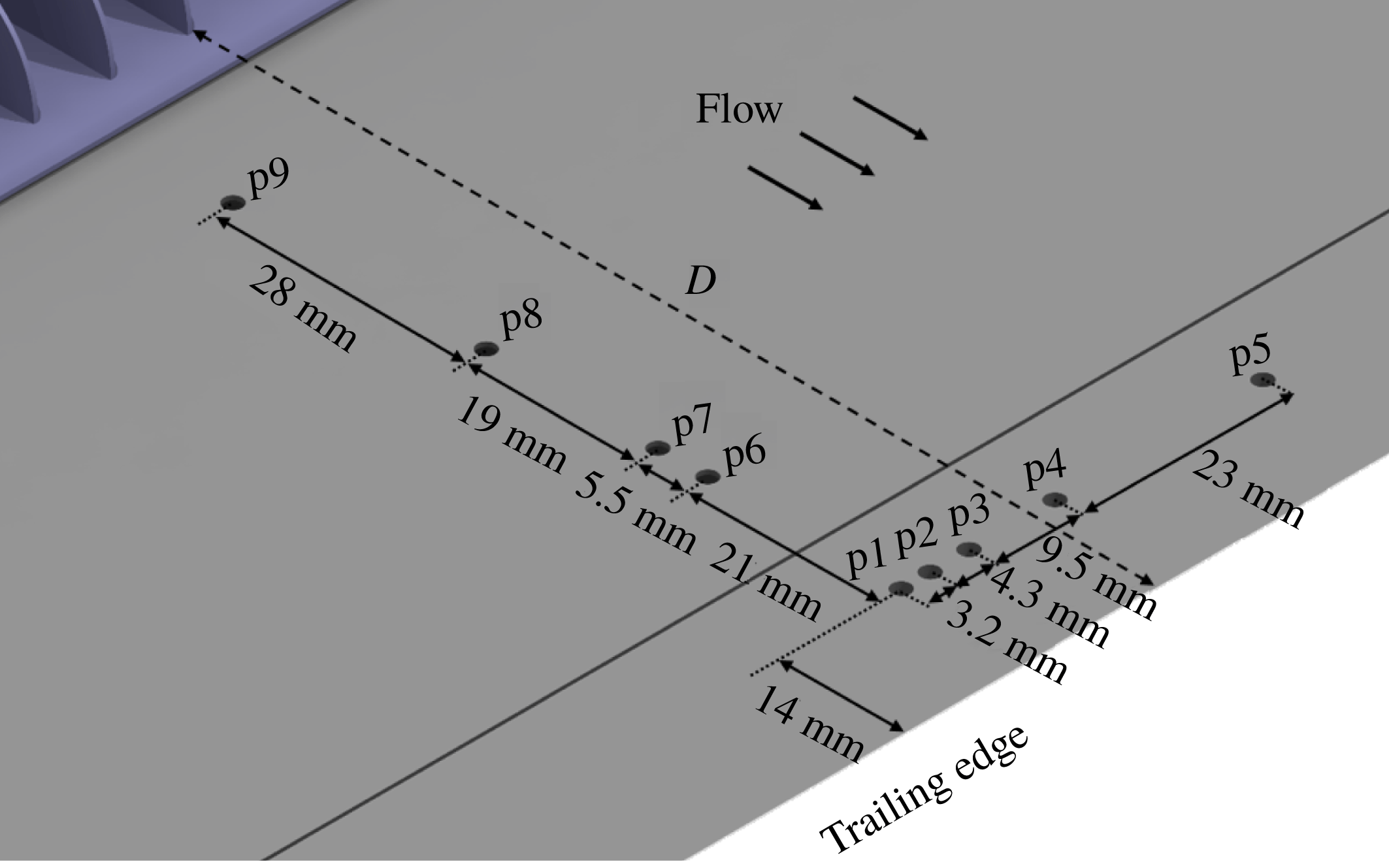
The layout of the surface pressure microphone array is depicted in figure 3. The locations of the pinholes on the upper surface of the flat plate are summarized in table 1. A total of nine microphones are arranged in the form of an L-shaped array on the surface of the flat plate. A set of microphones are distributed in the streamwise direction from
 $x/c=0.849$
to
 $0.976$
to provide information on the convection velocity of the turbulent eddies. Another set of microphones are positioned along the span to measure the spanwise coherence and length scale of the boundary layer turbulent structures. The spanwise microphones are distributed with unequal separation distances, according to the potential function
 $z/z_{min}=(z_{max}/z_{min})^{(i-2)/(N-2)},~i=2,\ldots ,N$
, in order to obtain a good range of distances with all pinhole pairs. The minimum and maximum lateral distances of the pinholes from the flat-plate midspan,
 $z_{min}$
and
 $z_{max}$
, are respectively 3.2 mm and 40 mm. Such an unequal distribution of the sensors leads to a non-redundant population of spacings and maximizes the number of spatial distances available for cross-correlation studies.
Many investigations have been carried out for proper measurement of the boundary layer surface pressure fluctuations and installation of miniature microphones (Corcos Reference Corcos1963; Willmarth & Roos Reference Willmarth and Roos1965; Ffowcs Williams & Hall Reference Ffowcs Williams and Hall1970; Brooks & Hodgson Reference Brooks and Hodgson1981; Schewe Reference Schewe1983; Gravante et al.
Reference Gravante, Naguib, Wark and Nagib1998; Blake Reference Blake2017). The finite size of the pressure transducers leads to the attenuation of the wall pressure fluctuation spectral levels at high frequencies, as reported by Corcos (Reference Corcos1963) and Willmarth & Roos (Reference Willmarth and Roos1965). In fact, the pressure measured by transducers of finite size is the average pressure applied across the transducer sensing area and therefore the pressure fluctuations with wavelength smaller than the transducer sensing area are spatially integrated. In order to resolve this issue, a small pinhole mask is often used to decrease the effective sensing area of the pressure transducer. Typically, the transducer sensing diameter, scaled based on the boundary layer inner layer variables,
 $d^{+}=du_{\unicode[STIX]{x1D70F}}/\unicode[STIX]{x1D708}$
, is used to determine whether or not the attenuation is significant. Schewe (Reference Schewe1983) concluded that
 $d^{+}<19$
is sufficient for the proper capturing of all essential wall pressure fluctuations. Later, Gravante et al. (Reference Gravante, Naguib, Wark and Nagib1998) reported that the maximum allowable non-dimensional sensing diameter to avoid spectral attenuation at high frequencies is in the range
 $12<d^{+}<18$
. The pinhole mask used for the current study for the free-stream velocities ranging from 10 to
 $20~\text{m}~\text{s}^{-1}$
gives a non-dimensional sensing diameter range of
 $10<d^{+}<20$
. Thus, the error due to the attenuation effects at high frequencies can be assumed negligible. However, the correction suggested by Corcos (Reference Corcos1963) has also been implemented to the data in order to account for any possible attenuation effects.
The L-shaped surface microphone array.

Position of the unsteady pressure pinholes on the flat plate.

Special care is taken in the selection of the streamwise distance of the spanwise microphones (p1 to p5) from the trailing edge. On the one hand, the streamwise distance between the microphone and the trailing edge must be small enough to be a true representative of the turbulence properties past the trailing edge; and on the other hand, it should not be too small, such that the spanwise length scale
 $\unicode[STIX]{x1D6EC}_{p,3}(f)$
and
 $\unicode[STIX]{x1D719}(f)$
, representing the statistical information about the incident pressure field, is affected by the scattering process at the trailing edge. Ffowcs Williams & Hall (Reference Ffowcs Williams and Hall1970) and Brooks & Hodgson (Reference Brooks and Hodgson1981) reported that the minimum sensor distance to the trailing edge where scattering effects can be neglected is approximately
 $\unicode[STIX]{x1D706}_{h}/2$
, where
 $\unicode[STIX]{x1D706}_{h}$
is the convected hydrodynamic wavelength of interest
 $(\unicode[STIX]{x1D706}_{h}=U_{C}/f)$
. Based on this criterion and the space constraint due to the thickness for the plate trailing edge, the spanwise pinholes are located at 14 mm upstream of the trailing edge (at
 $x/c=0.976$
).
2.4 Surface treatments
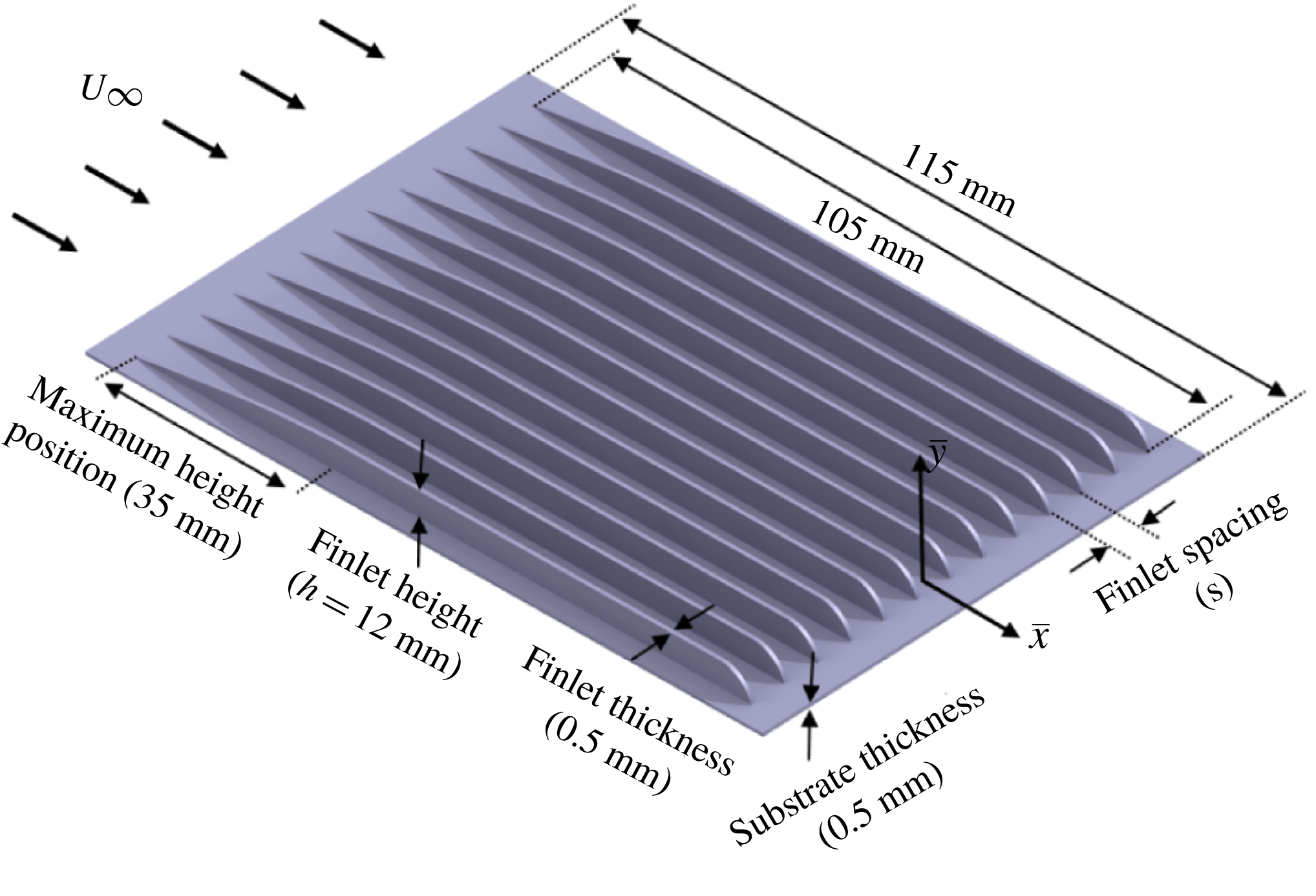
In the present study, blade-shaped fences (finlets) are chosen as the surface treatments for the flat plate. The general schematic and design parameters of a typical finlet are provided in figure 4. The finlets are supported by thin substrates with a thickness of 0.5 mm, glued to the flat plate. The leading and trailing edges of the substrate are faired to the flat-plate surface by covering it with a 0.1 mm thick aluminium tape. The substrate and tape will have an overall thickness of 0.6 mm, corresponding to
 $y^{+}=31$
, at the free-stream velocity of
 $20~\text{m}~\text{s}^{-1}$
. The surface treatment is placed on the top side of the plate, upstream of the trailing edge. The first part of the fences follows the turbulent boundary layer profile, i.e.
 $\hat{x}^{4/5}$
(
 $\hat{x}$
begins from the finlet leading edge) to avoid sudden abrupt changes to the boundary layer. To investigate the effects of finlet spacing, a total of six standard surface treatments with finlet spacings of
 $s=12,8,4,2,1$
and 0 mm (solid section), with a height of
 $h=12~\text{mm}$
, were fabricated using three-dimensional (3-D) rapid prototyping. In the following, the finlet surface treatments will be referred to as s12, s8, s4, s2, s1 and s0.
Blade-shaped finlet design parameters.

2.5 Measurement procedure
The boundary layer velocity measurements have been carried out using a single constant-temperature hot-wire anemometer. The sensing element of the probe is a standard
 $5~\unicode[STIX]{x03BC}\text{m}$
diameter tungsten wire with a length of 1.25 mm. The probe was calibrated by a standard Pitot tube located parallel to the incoming flow. Furthermore, the frequency response of the probe was verified by means of a square wave test to ensure a second-order response and demonstrating a
 $-3~\text{dB}$
drop-off, based on the definition of Freymuth (Reference Freymuth1967), at 30 kHz, for the free-stream mean velocity of
 $U_{\infty }=20~\text{m}~\text{s}^{-1}$
. The probe is traversed in the boundary layer using a three-axis traverse unit controlled by stepper motors with 0.01 mm accuracy. The traverse unit allowed continuous movement in the streamwise (
 $x$
), spanwise (
 $y$
) and vertical (
 $z$
) directions. The data were recorded at a sampling frequency of 40 kHz and for a sampling time of 10 s. The spanwise flow velocity measurements confirmed an approximate 300 mm extent of uniform 2-D flow conditions at
 $x=566~\text{mm}$
(
 $x/c=0.976$
) along the plate span. The near-wall mean velocities and the skin friction coefficient are estimated using Spalding’s equation,
 $$\begin{eqnarray}y^{+}=u^{+}+\text{e}^{-\unicode[STIX]{x1D705}B}[\text{e}^{\unicode[STIX]{x1D705}u^{+}}-1-\unicode[STIX]{x1D705}u^{+}-(\unicode[STIX]{x1D705}u^{+})^{2}/2-(\unicode[STIX]{x1D705}u^{+})^{3}/6],\end{eqnarray}$$
where
 $u^{+}=u/u_{\unicode[STIX]{x1D70F}}$
,
 $y^{+}=yu_{\unicode[STIX]{x1D70F}}/\unicode[STIX]{x1D708}$
, and
 $\unicode[STIX]{x1D705}$
and
 $B$
are the von Kármán and an additive empirical constant, which are chosen to be 0.41 and 5.0, respectively (Spalding Reference Spalding1961). Spalding’s formulation is a power-series interpolation scheme joining the linear sublayer to the logarithmic region, and the friction velocity (
 $u_{\unicode[STIX]{x1D70F}}$
) is obtained by fitting the measured data to the logarithmic region of Spalding’s equation (Kendall & Koochesfahani Reference Kendall and Koochesfahani2006). Furthermore, to assess the measured mean velocity profile in the outer wake region, Coles’ log-wake law (Coles Reference Coles1956) has been used, defined as
 $$\begin{eqnarray}u^{+}=\frac{1}{\unicode[STIX]{x1D705}}\ln y^{+}+B+\frac{2\unicode[STIX]{x1D6F1}_{w}}{\unicode[STIX]{x1D705}}\sin ^{2}\left(\frac{\unicode[STIX]{x03C0}y}{2\unicode[STIX]{x1D6FF}}\right).\end{eqnarray}$$
The last term in (2.2) is Coles’ wake function (Coles Reference Coles1969) and it takes into account the effect of adverse pressure gradient (APG) on the mean streamwise velocity component. The pressure gradient parameter,
 $\unicode[STIX]{x1D6F1}_{w}=0.8(\unicode[STIX]{x1D6FD}+0.5)^{3/4}$
, is a function of wall shear stress
 $\unicode[STIX]{x1D70F}_{w}$
and the local pressure gradient
 $\text{d}C_{p}/\text{d}x$
, with
 $\unicode[STIX]{x1D6FD}=(\unicode[STIX]{x1D6FF}^{\ast }/\unicode[STIX]{x1D70F}_{w})\,\text{d}C_{p}/\text{d}x$
(Durbin & Reif Reference Durbin and Reif2011), which is zero in the case of a clean flat plate.
To calculate the uncertainty of the hot-wire data, the methodology provided by Yavuzkurt (Reference Yavuzkurt1984) is used. The independent parameters such as the atmospheric temperature and pressure, curve fitting error in the calibration, analogue/digital resolution uncertainty, probe positioning and humidity are considered for the uncertainty analysis. The results revealed that the maximum uncertainties in the measured mean velocity and turbulence intensity are approximately 3 %.
The unsteady surface pressure measurements were performed using miniature microphones (Knowles FG-23329-P07). A tube with a length of 110 mm and diameter of 10 mm along with a high-quality loudspeaker were used for the calibration of the microphones (Maryami et al.
Reference Maryami, Azarpeyvand, Dehghan and Afshari2019). A
 $1/4$
inch 40BP GRAS microphone, calibrated with a GRAS sound calibrator type 42AB, was used as the reference microphone. The calibration results showed that the sensitivity of the FG-23329-P07 microphones varied approximately between 20 and
 $24.1~\text{mV}~\text{Pa}^{-1}$
. To provide a transfer function for each microphone, all microphones were calibrated in situ with a white noise excitation signal over the frequency range of 100 Hz to 20 kHz. The attenuation and possible resonances induced by the L-shaped channel used to connect the microphones to the pinholes on the surface are therefore accounted for by the in situ calibration. The method employed in the calibration of the FG-23329-P07 microphones is based on the calibration procedure proposed by Mish (Reference Mish2001). The microphones were powered by a 10-channel power module and the data were collected by a 16-channel NI PCI-6023E data acquisition system, at the sampling frequency of
 $f_{s}=40~\text{kHz}$
, for 20 s. The spectral analysis of the recorded data is done using the Pwelch power spectral density (PSD) function in MATLAB with a Hamming window function and 50 % overlap. Reliable and repeatable measurements are achieved for all microphones. The experimental uncertainty for the surface pressure spectra is mainly due to the statistical convergence error, which is inversely proportional to the number of records used (Bendat & Piersol Reference Bendat and Piersol2011). To reduce such errors, in the present study, the spectra were calculated as the average of the spectra of individual data records obtained from dividing the pressure time series into a sequence of smaller records. In the current study, a total number of records used was
 $N_{r}=800$
resulting in an uncertainty of approximately 3.5 %.
3 Untreated (or clean) flat-plate results
In order to assess the validity of the measurements and to ensure that a fully turbulent ZPG boundary layer condition can be obtained using the flat-plate test rig, various flow quantities are investigated in this section. Results will be provided for the streamwise mean pressure distribution, boundary layer velocity profile, surface pressure PSD, lateral coherence (
 $\unicode[STIX]{x1D6FE}^{2}$
) and the eddy convection velocity.
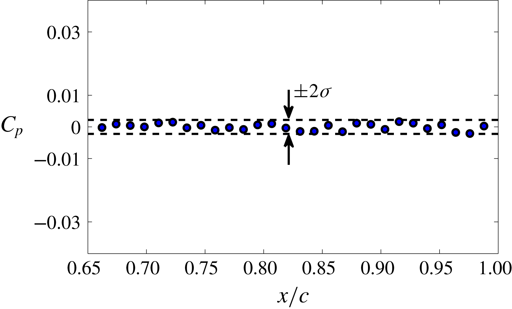
To ensure having ZPG condition on the upper surface of the model, especially in the vicinity of the trailing edge, it is necessary to assess the mean pressure distribution along the flat-plate chord. As can be seen, the measured pressure coefficient,
 $C_{p}$
, along the flat-plate chord between
 $x/c\approx 0.66$
(
 $x=384~\text{mm}$
) and
 $x/c\approx 0.99$
(
 $x=573~\text{mm}$
) is constant to within
 $\pm 0.22\,\%$
, as shown in figure 5, where
 $\unicode[STIX]{x1D70E}$
is the standard deviation.
Pressure coefficient (
 $C_{p}$
) distribution in the streamwise direction between
 $0.66\leqslant x/c\leqslant 0.99$
for the clean flat plate for a free-stream velocity of
 $20~\text{m}~\text{s}^{-1}$
.

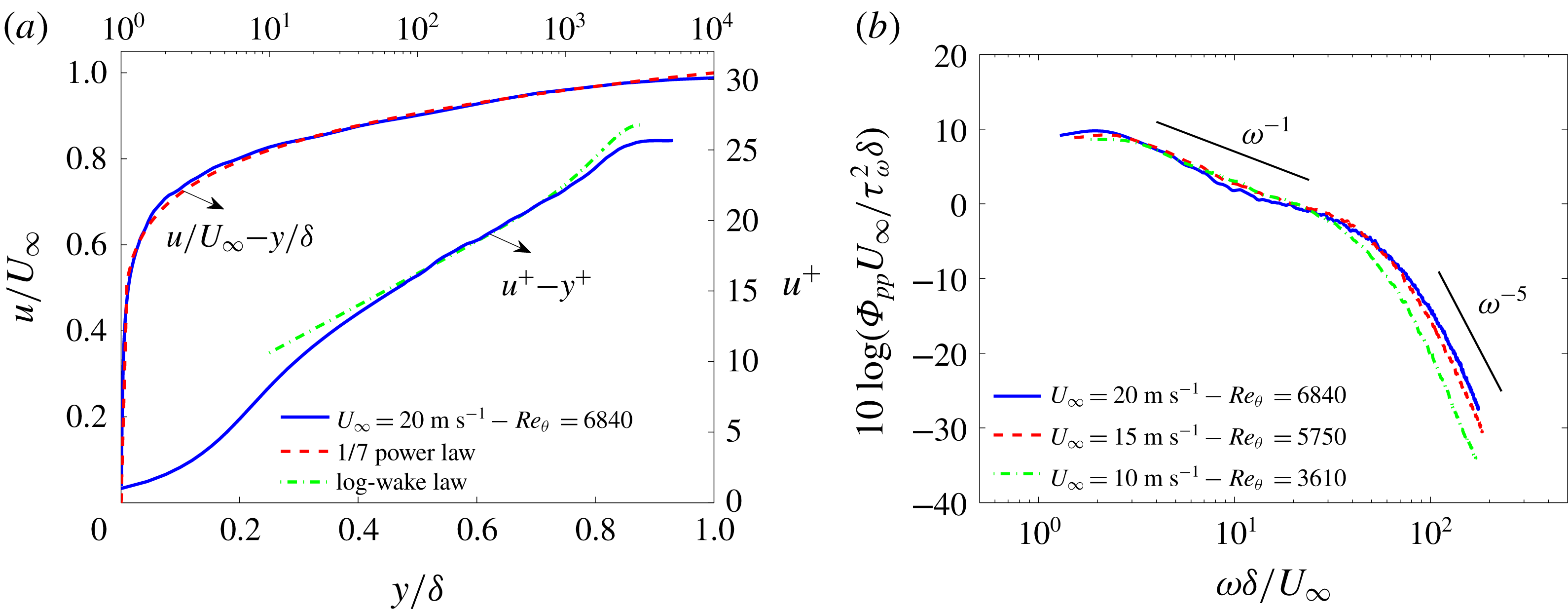
(a) Turbulent boundary layer mean velocity profiles in outer and inner scaling and comparison with the results predicted by the
 $1/7$
power law and Coles’ log-wake law. (b) Surface pressure spectra scaled by
 $\unicode[STIX]{x1D70F}_{w}$
as pressure scale and
 $\unicode[STIX]{x1D6FF}/U_{\infty }$
as time scale at the position of microphone p1 (
 $x/c=0.976$
) at
 $20~\text{m}~\text{s}^{-1}$
.

In figure 6(a), the mean velocity profiles for the clean flat plate are shown in the inner–outer layer scales at
 $x=566~\text{mm}$
(
 $x/c=0.976$
) at
 $20~\text{m}~\text{s}^{-1}$
. As can be seen in figure 6(a), the velocity profile in the outer scaling format shows acceptable agreement with the
 $1/7$
power-law turbulent boundary layer profile. The velocity profile based on the inner scaling also shows good agreement in a different boundary layer region. The small discrepancies observed in the outer region of the flow are due to the use of a physical trip device. The result has shown that, while the near-wall region recovers to a canonical behaviour, the outer wake region result is lower than Coles’ log-wake law prediction (Coles Reference Coles1956). This is, however, in agreement with the observations made by Schlatter & Örlü (Reference Schlatter and Örlü2012) and Marusic et al. (Reference Marusic, Chauhan, Kulandaivelu and Hutchins2015), who demonstrated that the near-wall region quickly adapts to that of a canonical boundary layer, while the outer layer, exhibiting stronger and long-lasting variations in the mean and variance profiles, requires a much longer development length to forget the specific tripping history.
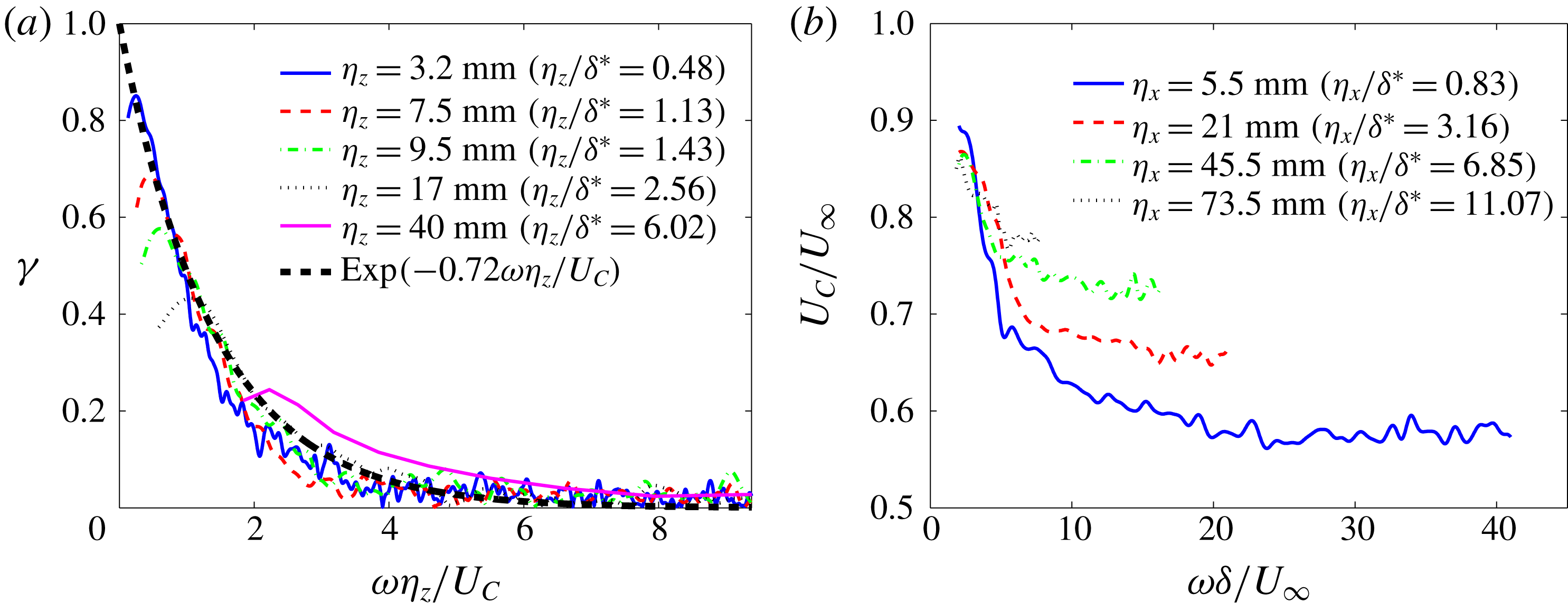
(a) Normalized lateral cross-spectra and (b) variation of eddy convection velocity with
 $\unicode[STIX]{x1D714}\unicode[STIX]{x1D6FF}/U_{\infty }$
and with distance between streamwise microphones for the clean flat plate at
 $20~\text{m}~\text{s}^{-1}$
.

The surface pressure PSD results were measured using the microphone p1 at
 $x/c=0.976$
, near the trailing edge of the flat plate. To evaluate the collapse of surface pressure PSD results, measurements were carried out for different free-stream velocities,
 $U_{\infty }=10$
, 15 and
 $20~\text{m}~\text{s}^{-1}$
. The microphone data are corrected based on the calibration procedure and the correction of Corcos (Reference Corcos1963) described in §§ 2.3 and 2.5. Results will only be presented in the frequency ranges where the pressure data collected are at least 10 dB higher than the background noise. Figure 6(b) provides results for normalized surface pressure PSD data as a function of the non-dimensional frequency,
 $\unicode[STIX]{x1D714}\unicode[STIX]{x1D6FF}/U_{\infty }$
. The PSD results have been normalized by using the wall shear stress (
 $\unicode[STIX]{x1D70F}_{w}$
) as the pressure scale, and
 $\unicode[STIX]{x1D6FF}/U_{\infty }$
as the time scale, as suggested by Goody (Reference Goody2004). The plot shows that surface pressure PSD decays at mid-frequencies,
 $\unicode[STIX]{x1D714}\unicode[STIX]{x1D6FF}/U_{\infty }$
, with a slope of
 $\unicode[STIX]{x1D714}^{-1}$
, which is slightly higher than the reported values in the literature for an ideal turbulent boundary layer. McGrath & Simpson (Reference McGrath and Simpson1987), Blake (Reference Blake1970) and Goody & Simpson (Reference Goody and Simpson2000) reported a mid-frequency pressure spectrum slope of
 $-0.7$
to
 $-0.8$
. This small difference in the wall pressure fluctuations can be attributed to the use of a physical trip device in our experiment. The curves also follow a decay rate of
 $\unicode[STIX]{x1D714}^{-5}$
at high frequencies, which agrees with the results reported in the literature (Goody Reference Goody2004; Hwang, Bonness & Hambric Reference Hwang, Bonness and Hambric2009). Based on the trends observed in figure 6(b), the surface pressure PSD results are the typical form for well-developed ZPG turbulent boundary layers, i.e. a high energy level in the low-frequency region, followed by an approximately steadily decreasing energy cascade region with slope of
 $\unicode[STIX]{x1D714}^{-1}$
at mid-frequencies, and a steep roll-off with slope of
 $\unicode[STIX]{x1D714}^{-5}$
at high frequencies.
Figure 7(a) shows the normalized lateral cross-spectra
 $\unicode[STIX]{x1D6FE}$
versus
 $\unicode[STIX]{x1D714}\unicode[STIX]{x1D702}_{z}/U_{C}$
measured between various spanwise microphones for the clean flat plate at
 $20~\text{m}~\text{s}^{-1}$
. Except for the values of
 $\unicode[STIX]{x1D714}\unicode[STIX]{x1D702}_{z}/U_{C}$
corresponding to the frequencies below the peak frequency, the coherence results tend to collapse onto a single curve of the form
 $\exp (-\unicode[STIX]{x1D6FD}\unicode[STIX]{x1D714}\unicode[STIX]{x1D702}_{z}/U_{C})$
. The exponential decay rate
 $\unicode[STIX]{x1D6FD}$
was found to be 0.72, which is consistent with the values reported in other references (Corcos Reference Corcos1964; Hu & Herr Reference Hu and Herr2016).
The convection velocity of the turbulent eddies in the boundary layer calculated using the phase analysis between the streamwise microphones near the trailing edge for the clean flat plate at
 $20~\text{m}~\text{s}^{-1}$
is presented in figure 7(b). The convective phase velocity of the wall fluctuating pressure field is defined by
 $U_{C}(\unicode[STIX]{x1D714},\unicode[STIX]{x1D702}_{x})=\unicode[STIX]{x1D714}\unicode[STIX]{x1D702}_{x}/\unicode[STIX]{x1D711}_{p_{i},p_{j}}(\unicode[STIX]{x1D714},\unicode[STIX]{x1D702}_{x})$
, where
 $\unicode[STIX]{x1D711}_{p_{i},p_{j}}(\unicode[STIX]{x1D714},\unicode[STIX]{x1D702}_{x})$
is the phase difference between two streamwise microphones separated by a streamwise distance of
 $\unicode[STIX]{x1D702}_{x}$
. Results will only be presented for the frequency ranges with high coherence between streamwise pressure sensors. As can be seen, the eddy convection velocity increases with increasing streamwise distance between the sensors (
 $\unicode[STIX]{x1D702}_{x}$
), while the non-dimensional frequency range over which the pressure field is coherent is reduced. The trends are consistent with those reported in the literature (Corcos Reference Corcos1964; Hu & Herr Reference Hu and Herr2016).
The main purpose of this section was to demonstrate that the flat-plate test rig used here with the flow tripping device can deliver a well-developed canonical turbulent boundary layer to be used for the rest of our surface treatment studies. The quantitative assessment presented in this section, including the streamwise mean pressure distribution, the boundary layer velocity profile, the surface pressure PSD, the lateral coherences and the convection velocity of the turbulent eddies in the boundary layer, has shown that the flat-plate test rig with the flow tripping device employed can deliver a good ZPG turbulent boundary layer, and that the mean and fluctuating quantities obtained here agree well with the prior experimental observations.
4 Treated flat-plate results
In this section, the boundary layer flow and surface pressure measurements carried out for the case of a flat plate treated with surface treatments (finlets) at zero angle of attack are presented. Measurements have been carried out for free-stream velocities of
 $U_{\infty }=10$
, 15 and
 $20~\text{m}~\text{s}^{-1}$
. However, results have been found to be independent of the Reynolds number in this velocity range and, therefore, data and discussions will be provided only for the free-stream velocity of
 $U_{\infty }=20~\text{m}~\text{s}^{-1}$
, for which we obtained high signal-to-noise ratio for surface pressure measurements.
4.1 Pressure field
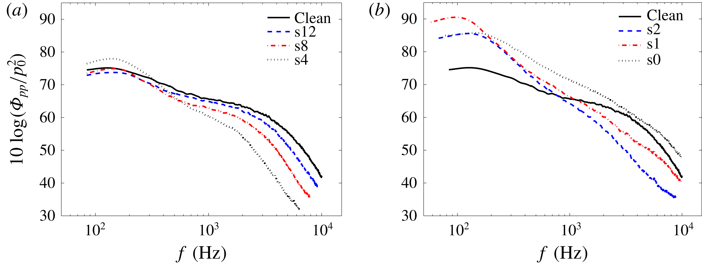
As noted in § 1, according to the mathematical models of Amiet (Reference Amiet1976) and Howe (Reference Howe1978), the surface pressure point spectrum in the vicinity of the trailing edge is a determining quantity for the prediction of the far-field trailing-edge noise. Figure 8 shows the surface pressure PSD measured by microphone p1 near the trailing edge (
 $x/c=0.976$
) of the clean and treated flat plates, normalized by
 $p_{ref}=20~\unicode[STIX]{x03BC}\text{Pa}$
. The microphone data are corrected according to the calibration procedure and the correction of Corcos (Reference Corcos1963) described in §§ 2.3 and 2.5. Six different finlet spacings,
 $s=12,8,4,2,1$
and 0 mm (i.e. a solid profile section) are considered. The results in figure 8 show the effects of the finlet spacing on the surface pressure PSD compared to the clean plate case. The results for the coarse (s12, s8, s4) and fine (s2, s1, s0) finlet spacings are presented in figure 8(a,b), respectively. As can be seen, the two finlet categories demonstrate very different surface pressure PSD behaviour. For the finlets with coarse spacing (s12 and s8), the presence of an upstream surface treatment generally leads to a significant reduction of the surface pressure over the mid- to high frequencies, with no noticeable changes to the low-frequency energy content of the boundary layer. By reducing the spacing between the finlets to 4 mm (s4), their effectiveness in reducing the surface pressure PSD at mid- to high frequencies increases (figure 8
a). However, further reducing the spacing seems to cause an undesirable increase in the low- and mid-frequency ranges, as shown in figure 8(b). For the cases with very fine spacing (s2 and s1), the results demonstrate that, while the presence of the upstream surface treatment leads to a reduction in the pressure PSD at high frequencies, it also results in a significant increase in low to mid-frequencies. These trends are consistent with the far-field noise observations of Clark et al. (Reference Clark, Alexander, Devenport, Glegg, Jaworski, Daily and Peake2017). The results of Clark et al. (Reference Clark, Alexander, Devenport, Glegg, Jaworski, Daily and Peake2017) showed that there exists a limit to the beneficial far-field noise effects of reducing the finlet spacing and that further reducing the spacing below a critical value can result in low-frequency increase of the far-field noise. The results in figure 8(a,b) also show that for the cases of s4 and s2 treatment, as well as the solid step (s0 case), a spectral broadband peak occurs at approximately 130 Hz, corresponding to the Strouhal number of
 $fh/U_{\infty }=0.078$
, where
 $h$
is the finlets height. This matches well with the non-dimensional vortex shedding frequency in the wake of a backward-facing step (BFS), which is reported in the literature to be approximately 0.07 (Lee & Sung Reference Lee and Sung2001; Liu, Kang & Sung Reference Liu, Kang and Sung2005). Furthermore, as can be seen, for the s1 finlet case the spectral peak occurs at
 $f=100~\text{Hz}$
, corresponding to
 $fh/U_{\infty }=0.06$
. This suggests that the boundary layer turbulence structures responsible for the broadband peak surface pressure PSD in the case of s1 are larger than that of s4, s2 and even s0. The underlying physics of this phenomenon will be further discussed in the following sections.
Surface pressure PSD referenced to
 $p_{ref}=20~\unicode[STIX]{x03BC}\text{Pa}$
measured by microphone p1 on the trailing edge of the clean and treated flat plates at
 $20~\text{m}~\text{s}^{-1}$
. This shows the effects of finlet spacing,
 $s$
, on surface pressure PSD: (a) coarse finlet spacing (s12, s8, s4), and (b) fine finlet spacing (s2, s1, s0).

The mean surface pressure distribution (
 $C_{p}$
) at various streamwise locations downstream of the surface treatments between
 $0.84\leqslant x/c\leqslant 0.99$
(
 $2.2\leqslant \bar{x}/h\leqslant 9.2$
) are presented in figure 9 for the clean and treated flat plates at the free-stream velocity of
 $20~\text{m}~\text{s}^{-1}$
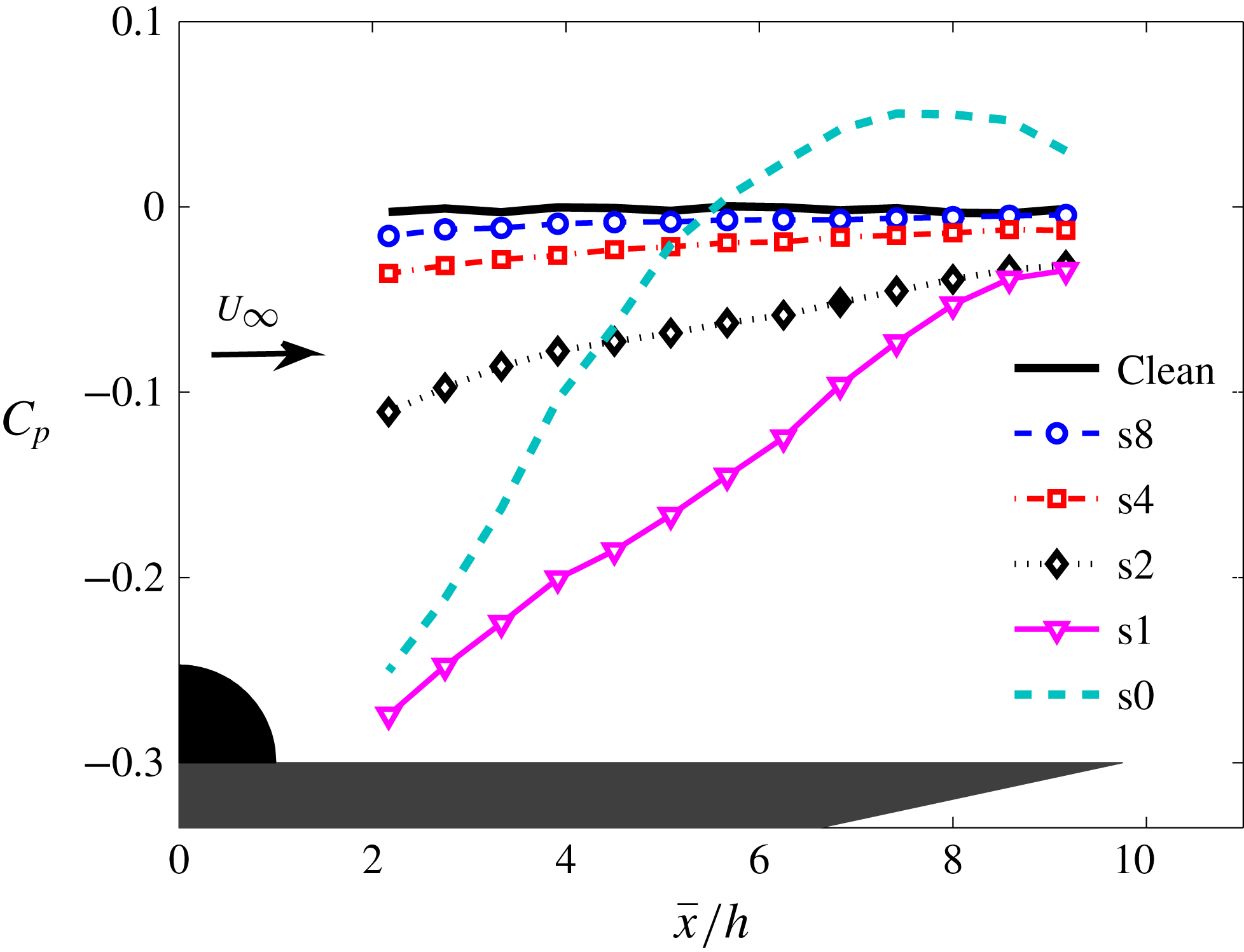
. It can be observed that the finlet treatments with coarse spacing (s8) induce a low level of pressure gradient downstream of the surface treatment area. However, reducing the spacing between the finlets leads to the emergence of an APG region behind the finlets. As can be seen, by reducing the spacing between the finlets, the flow tends to behave similar to an s0 case (solid profile). The shape of the pressure distribution curve for the s0 case is similar to those found in other investigations for a BFS (Farabee & Casarella Reference Farabee and Casarella1986). As shown, for the s0 case, in contrast to the standard ZPG condition expected for the clean flat plate, a localized APG exists immediately behind the step due to the emergence of a recirculation region. A maximum positive pressure is observed near the flow reattachment area, at
 $\bar{x}/h\approx 7$
, where the shear layer from the finlets interacts with the plate surface. The flow-field results will be provided in § 4.2. Downstream of the reattachment point, the pressure distribution is favourable, gradually converging back to the values expected for the clean flat plate. For the fine finlets (s2, s1), on the other hand, the slope of the pressure gradient is lower than in the s0 case and the maximum pressure coefficient occurs farther downstream at
 $\bar{x}/h\approx 9$
. In the case of the s0 BFS case, the results show that a negative large base pressure coefficient yields a more rapid turning of the flow towards the surface than the coarse finlet cases. The flow field in the case of the s2 finlet treatment, on the other hand, exhibits a lower base pressure, resulting in a longer reattachment distance. Furthermore, the
 $C_{p}$
results show that the negative pressure values observed for the case of the s1 treatment are even greater than that of the s0 case. This, along with the surface pressure fluctuation results presented in figure 8(b), supports the idea that the s1 case has a different physics from that of s0 and the coarser cases. This will be further discussed in the following sections.
Pressure coefficient (
 $C_{p}$
) distribution in the streamwise direction for the clean and treated flat-plate cases, between
 $2.2\leqslant \bar{x}/h\leqslant 9.2$
at the free-stream velocity of
 $20~\text{m}~\text{s}^{-1}$
.

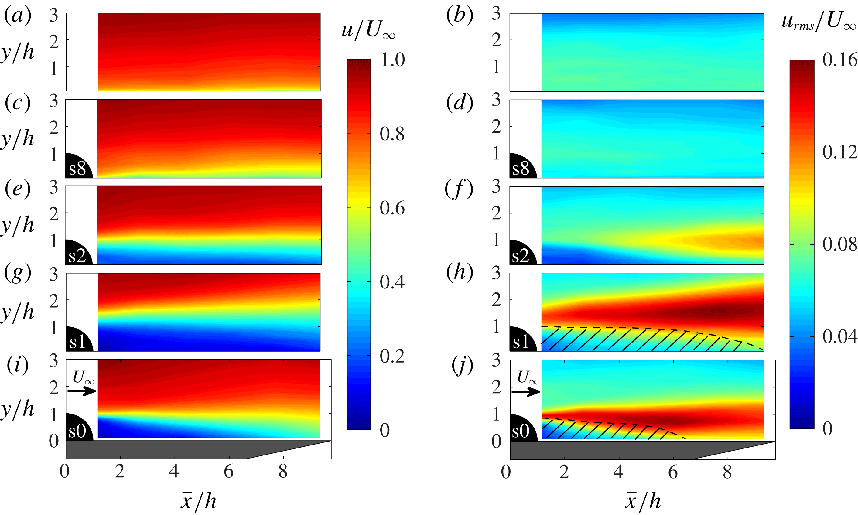
Boundary layer mean and r.m.s. velocity contour map downstream of the various surface treatments at
 $20~\text{m}~\text{s}^{-1}$
: (a,b) clean flat plate, (c,d) s8, (e, f) s2, (g,h) s1, (i, j) s0 (BFS).

4.2 Boundary layer flow field
To gain a better insight into the mechanisms through which both the coarse and fine finlet treatments affect the boundary layer flow structures, velocity measurements have been carried out downstream of the surface treatment section and near the trailing edge of the flat plate. In figure 10, the contour maps of the dimensionless mean velocity and turbulence intensity (
 $u_{rms}/U_{\infty }$
) downstream of the surface treatments for the coarse (s8) and fine (s2, s1) finlet spacings are shown and compared to the clean flat-plate results. The results for a BFS (s0) with similar geometrical profile as the finlets are also presented for comparison. It should be noted that for the BFS (s0) and s1 cases, the local turbulence intensity, i.e.
 $u_{rms}/u$
, may exceed 30 % within the shear layer and the reversed flow regions and therefore, as reported in the literature (Bruun Reference Bruun1995; Badran & Bruun Reference Badran and Bruun1999), rectification errors become significant and the hot-wire measurements can be considered inaccurate. The regions where
 $u_{rms}/u>0.3$
are shown as cross-hatched areas. Figure 10 shows that the presence of the finlets with coarse spacing (s8) leads to a reduction of both the mean velocity and turbulence intensity in the near-wall region downstream of the finlets compared to the clean plate case. It is hypothesized that, in the case of finlets with coarse spacing, boundary layer flow is channelled between the finlets, leading to an increased wetted surface area and therefore possible increase in energy dissipation via surface friction. The contour maps of the mean velocity and turbulence intensity downstream of the s2 and s1 treatment cases show that, for the fine finlets, the flow behaves nearly like the flow behind a BFS (s0). The two-dimensional BFS is one of the most studied geometries for separated flows and it has been the subject of numerous experimental and numerical investigations, as reviewed by Bradshaw & Wong (Reference Bradshaw and Wong1972) and Eaton & Johnston (Reference Eaton and Johnston1981). The flow field for the BFS is characterized as having a well-defined separation point at the top of the step. Owing to the Kelvin–Helmholtz instability, small-scale vortices in the shear layer roll up and pair with the adjacent vortices to form larger coherent structures (Troutt, Scheelke & Norman Reference Troutt, Scheelke and Norman1984). These large coherent structures shed and convect downstream after attaining the maximum length scale, i.e. the step height. The issue of small vortices pairing up will be further discussed later in the case of finlets with coarse and fine spacings. As expected, in figure 10(i, j), a thin free shear layer is formed which extends downstream to the reattachment point at approximately
 $\bar{x}/h\approx 6{-}7$
. It is well known that beneath the free shear layer, the recirculating flow forms a separation bubble. The flow reattachment to the bottom wall is due to the APG in the wake of the BFS, as observed in figure 9. It should be noted that the downstream growth and reattachment position of the shear layer are dependent on various parameters, including the ratio of the inflow boundary layer thickness to the step height, Reynolds number, inlet turbulence intensity, step aspect ratio, etc. (Bradshaw & Wong Reference Bradshaw and Wong1972).
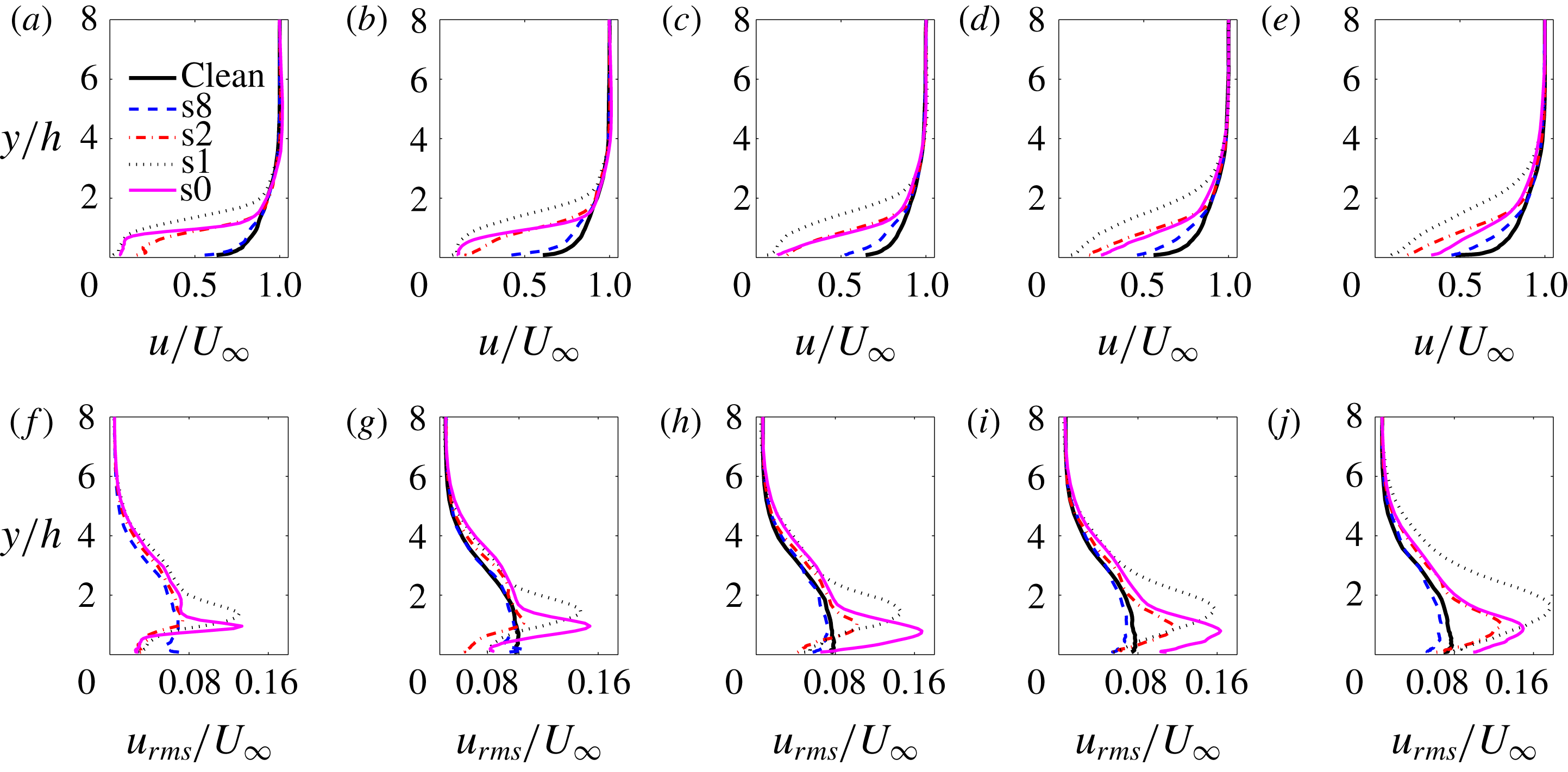
Boundary layer mean and r.m.s. velocity profiles at different streamwise location downstream of the various surface treatments: (a, f)
 $\bar{x}/h=1.1$
, (b,g)
 $\bar{x}/h=2.5$
, (c,h)
 $\bar{x}/h=4.8$
, (d,i)
 $\bar{x}/h=6.8$
, (e, j)
 $\bar{x}/h=8.6$
.

Figure 10(e, f) present the contour plots of the mean velocity and turbulence intensity downstream of the finlets with fine spacing (s2 case). As can be seen, similar to the BFS case (s0), the separated flow forms a shear layer at approximately
 $y/h\approx 1$
. However, the maximum turbulence intensity occurs farther downstream, compared to the BFS case, at
 $\bar{x}/h\approx 9$
. This agrees with the shift of the maximum pressure coefficient position for the s2 case observed in figure 9, and is believed to be due to the flow leaking through the finlets. This behaviour is also consistent with the observations of Cassiani, Katul & Albertson (Reference Cassiani, Katul and Albertson2008) and Markfort, Porté-Agel & Stefan (Reference Markfort, Porté-Agel and Stefan2014) for complex porous plant canopies and Liu et al. (Reference Liu, Ke, Chen and Sung2006) for an open BFS, in which the reattachment length was observed to be altered in the presence of low-speed exit flow compared to the standard simple BFS. Further decreasing the spacing between the finlets to 1 mm (s1) seems to cause the emergence of a stronger free shear layer that occurs much farther away from the plate surface (figure 10
g,h). The flow behaviour observed for the s1 case is also consistent with the greater negative mean surface pressure values observed in figure 9, and the higher surface pressure spectral peak observed in figure 8(b).
To better understand the flow behaviour downstream of both the coarse (s8) and fine (s2, s1) surface treatments, the boundary layer mean velocity (
 $u/U_{\infty }$
) and the turbulent intensity (
 $u_{rms}/U_{\infty }$
) profiles are presented in figure 11 for the clean and some treated flat-plate cases at several streamwise locations (
 $\bar{x}/h=1.1$
to 8.6). The results show that all surface treatments create a velocity deficit, indicating significant changes to the boundary layer structures downstream of the finlet treatments. As seen, the variations in the boundary layer mean velocity deficit increases with decreasing the space between the finlets. These results are consistent with the observations made for the flow behind plant canopies (Finnigan Reference Finnigan2000; Cassiani et al.
Reference Cassiani, Katul and Albertson2008) and for the flow downstream of windbreaks (Plate Reference Plate1971; Raine & Stevenson Reference Raine and Stevenson1977). In both cases, it was shown that, as the permeability of the porous barrier is reduced, the mean velocity in the near wake decreases. As can be seen, in the presence of the finlets with coarse spacing (s8), the mean velocity and the turbulent intensity profiles are reduced in the near-wall region,
 $y/h<2$
, at all streamwise locations downstream of the finlets. The mean and root-mean-square (r.m.s.) velocity reduction observed in the case of s8 finlets is believed to be due to the changes to the structure of the boundary layer as they pass over and through the s8 channels and the increased wetted surface area.
The boundary layer mean velocity results, alongside their contour maps in figure 10, show that in the presence of the finlets with fine spacing (s2, s1), the flow downstream of the finlets behaves somewhat like the flow behind a BFS (s0). Despite the obvious similarities, there however exist significant differences between the two cases. In the case of the s2 finlet (at
 $\bar{x}/h=1.1$
), one can see the air flow exiting the finlet sections into the wake region of the finlets (
 $y/h<1$
). In that sense, the finlet treatments with fine spacing (s2) can be considered as a step with a unidirectional streamwise permeability. In the case of the s1 finlet case, on the other hand, no significant flow leakage into the finlets wake can be seen (similar to the s0 case) and the separated flow forms a shear layer farther away from the surface (
 $y/h\approx 1.7$
) compared to the s0 BFS case. This suggests that in the case of the s1 treatment, the boundary layer flow entrapped within the finlet channels leaves the channels through the upper surface of the finlets, causing the shear layer to move away from the surface, leading to a late reattachment and the emergence of larger turbulence structures. This then results in an increase in the low-frequency energy content of the surface pressure PSD, as observed in figure 8. This behaviour is consistent with the observations made by Cassiani et al. (Reference Cassiani, Katul and Albertson2008) for the flow field inside plant canopies. The results of Cassiani et al. (Reference Cassiani, Katul and Albertson2008) showed that, while for plant canopies with high permeability, equivalent to large finlet spacing, no recirculation zones were observed within the canopy, reducing the permeability of the porous canopy led to the emergence of a recirculation zone inside the canopy.
The r.m.s. velocity results can also provide some useful information about the effect of finlets on the boundary layer structures. In the case of finlets with fine spacing, the reduction in the r.m.s. velocity is believed to be partly due to the emergence of a flow recirculation area behind the finlets, as seen in figure 10 and partly due to the low-momentum flow leaving the finlet channels and entering the finlets wake region. In order to better assess the contribution of the two mechanisms to the overall reduction of the energy content of the flow within the finlets wake for the s2 and s1 cases, their r.m.s. velocity profiles are compared against that of the BFS case (s0) at several streamwise locations (
 $\bar{x}/h\approx 1.1$
to 8.6). The strong r.m.s. velocity peak at
 $y/h\approx 1$
for the BFS case (s0) corresponds to the location of a shear layer, originating from the top surface of the step. As can be seen in figure 11(f), for the s2 case, at the first position immediately after the finlet treatments (
 $\bar{x}/h=1.1$
), no noticeable increase in the r.m.s. velocity can be observed at
 $y/h\approx 1$
, indicating the absence of a strong shear layer from the top surface of the finlets. Therefore, the reduction in the energy content of the flow structures in the near-wall regions (
 $y/h<1$
) is believed to be mostly due to the low-momentum flow exiting the finlet channels. Further reducing the finlet spacing (s1) leads to the emergence of a strong peak at
 $y/h\approx 1.7$
and also the disappearance of the flow entering the finlet wake through the channels. Therefore, in the case of the s1 finlets, the emergence of the flow recirculation behind the finlets is the main reason for the reduction of the r.m.s. velocity in the near-wake region (
 $\bar{x}/h=1.1$
).
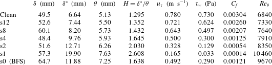
Table 2 summarizes some of the important boundary layer parameters for the clean and treated flat plate near the trailing edge at
 $x/c=0.976$
, at the free-stream flow speed of
 $U_{\infty }=20~\text{m}~\text{s}^{-1}$
. The boundary layer quantities for the solid step case (s0) are also provided for comparison. The near-wall mean velocity and skin friction coefficient are estimated based on Spalding’s equation described in § 2.5. It should be noted that, although the flow reattaches to the surface in the vicinity of the trailing edge for the fine finlets and behaves somewhat similar to an equilibrium boundary layer, some care must be taken when using Spalding’s equation due to the non-equilibrium boundary layer formed downstream of the finlets. As can be seen, in the case of treated plates, the displacement thickness (
 $\unicode[STIX]{x1D6FF}^{\ast }$
), the momentum thickness (
 $\unicode[STIX]{x1D703}$
) and the shape factor (
 $H$
) are larger than those of the clean plate case, and these effects are intensified with decreasing finlet spacing. The results also show that the skin friction coefficient (
 $C_{f}$
) decreases as a result of the introduction of an upstream surface treatment and that reducing the finlet spacing further reduces the skin friction coefficient. More importantly, the results for the s1 and s2 treatments have shown that, while their boundary layer thickness (
 $\unicode[STIX]{x1D6FF}$
) is slightly smaller than that of the s0 step case, their displacement and momentum thickness, as well as the shape factor, increase significantly, which is consistent with the velocity deficit observations in figure 11(e). Similar observations were also made in the case of a porous canopy BFS (Markfort et al.
Reference Markfort, Porté-Agel and Stefan2014).
Boundary layer parameters for treated and clean flat-plate cases at
 $x/c=0.976$
and
 $U_{\infty }=20~\text{m}~\text{s}^{-1}$
.

4.3 Boundary layer energy content
In order to better understand the changes to the boundary layer flow structures due to the presence of the proposed surface treatments, the energy content of the turbulence structures within the boundary layer has been investigated. The velocity PSD has been measured for the clean and treated flat-plate cases at several streamwise locations between
 $\bar{x}/h=2.5$
and 8.6, at
 $U_{\infty }=20~\text{m}~\text{s}^{-1}$
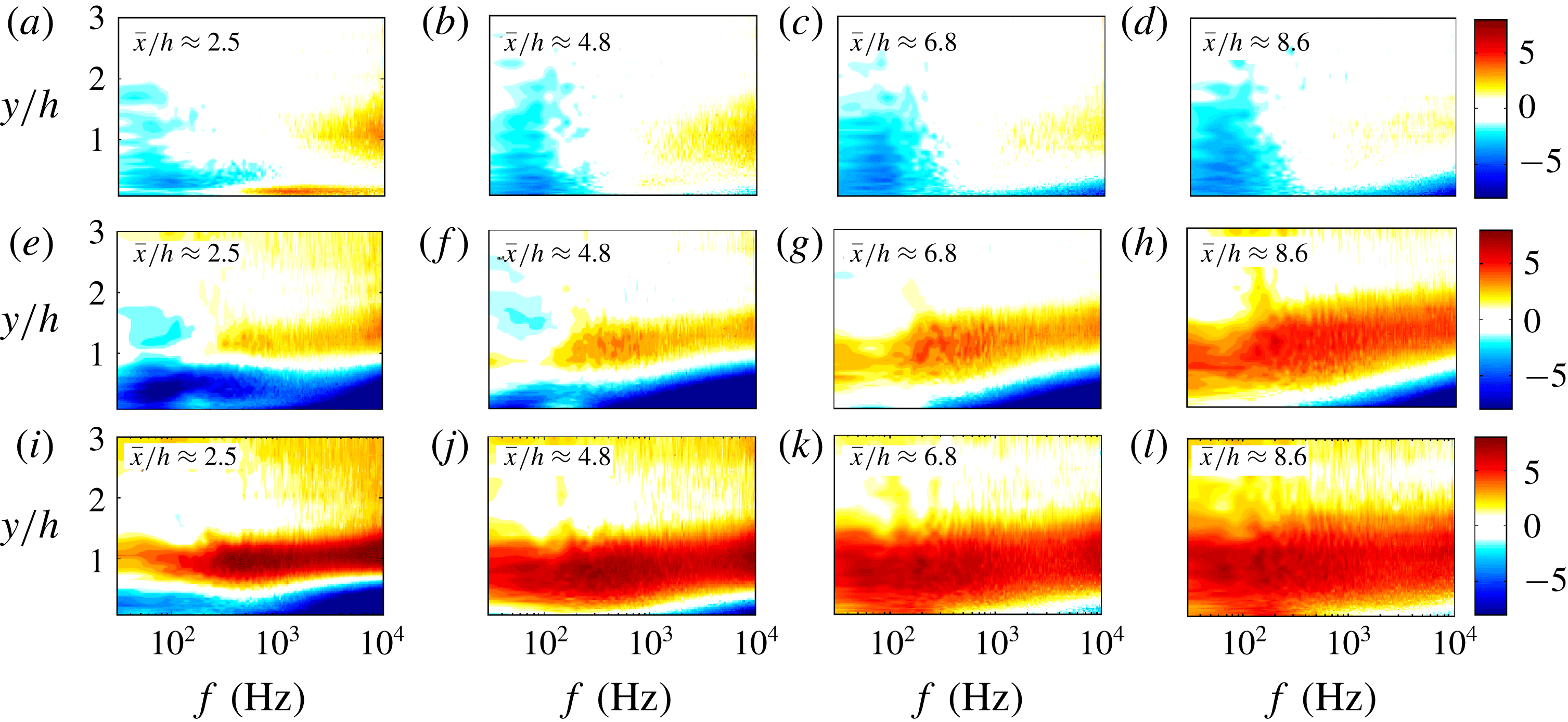
. The results presented in figure 12 show the velocity PSD contour plots, normalized by that of the clean flat plate (
 $\unicode[STIX]{x0394}\unicode[STIX]{x1D719}_{uu}=10\log _{10}(\unicode[STIX]{x1D719}_{uu,treated}/\unicode[STIX]{x1D719}_{uu,clean})$
). The results in figure 12(a)–(d) clearly show that the use of the s8 finlets leads to a reduction of the low-frequency energy content of the boundary layer structures over the whole vertical distance from the plate, up to approximately twice the height of the finlet, at all streamwise locations downstream of the finlets. This also supports the earlier claim that the s8 finlet treatment tends to reduce the turbulence intensity at all streamwise positions behind the finlets (see figure 11). Furthermore, it can be observed that the energy content of the near-wall high-frequency structures has been reduced at nearly all streamwise locations, except in the very near-wake region, i.e.
 $\bar{x}/h=2.5$
, which is attributed to the 0.5 mm treatment substrate, as also seen in figure 11. The results also show an area of high-frequency structures at
 $\bar{x}/h=2.5$
and
 $y/h\approx 1$
, due to a relatively weak free shear layer originating from the upper surface of the finlets. Progressing downstream, these high-frequency structures fail to grow to form larger coherent structures and gradually fade away (Winant & Browand Reference Winant and Browand1974). This can be due to the presence of a strong exit flow behind the s8 finlets. It can also be seen that, for the s8 finlets at the further downstream locations (
 $\bar{x}/h=6.8$
to 8.6), the overall structure of the boundary layer remains approximately unchanged, which is consistent with the results seen in figure 11.
The normalized velocity PSD results for the s2 finlet treatment at different axial locations are presented in figure 12(e)–(h). The results in figure 12(e) (at
 $\bar{x}/h=2.5$
) show that the energy content of the turbulent flow structures reduces in the areas near the wall (
 $y/h<1$
) over the whole frequency ranges. Furthermore, the use of finlets has led to a significant increase in the high-frequency energy content of the flow structures at around
 $y/h\approx 1$
, which is due to a strong flow separation caused by the finlets upper surface, as also evidenced by the mean velocity gradients in figure 11(b) and the turbulence intensity peaks in figure 11(g). As seen, the shear layer originating from the top surface of the s2 treatment is much stronger than that of the s8 treatment, which is due to its larger surface area in contact with the flow. Immediately after the s2 treatment at
 $\bar{x}/h=2.5$
, the shear layer is still quite thin and therefore the energy content is of high-frequency nature. Moving further downstream, the shear layer becomes wider and stronger, covering a wider frequency range, similar to the s0 BFS case (see figure 12
i–l). Furthermore, the distribution of the turbulent energy in the shear layer region at different streamwise positions indicates a transfer of fluctuation energy to lower frequencies through the vortex coalescence mechanism, as discussed for the case of a BFS by Roos & Kegelman (Reference Roos and Kegelman1986). Lastly, as a result of this energy transfer at around
 $y/h\approx 1$
, the turbulent energy reduction of the finlets in the vicinity of the flat-plate trailing edge (
 $\bar{x}/h=8.6$
) is limited to the near-wall high-frequency structures. Furthermore, the comparison between figures 12(h) and (l), corresponding to
 $\bar{x}/h=8.6$
, shows that, in contrast to the s2 finlet treatment, there is no considerable reduction in the energy content of the near-wall high-frequency structures for the s0 BFS case and this is consistent with the surface pressure spectra observations in figure 8(b).
Normalized velocity PSD,
 $\unicode[STIX]{x0394}\unicode[STIX]{x1D719}_{uu}=10\log _{10}(\unicode[STIX]{x1D719}_{uu,treated}/\unicode[STIX]{x1D719}_{uu,clean})$
, contour plots for treated flat plates at several streamwise locations (
 $\bar{x}/h=2.5$
to 8.6): (a–d) s8 treatment, (e–h) s2 treatment, (i–l) s0 BFS.

4.4 Spanwise coherence and correlation length
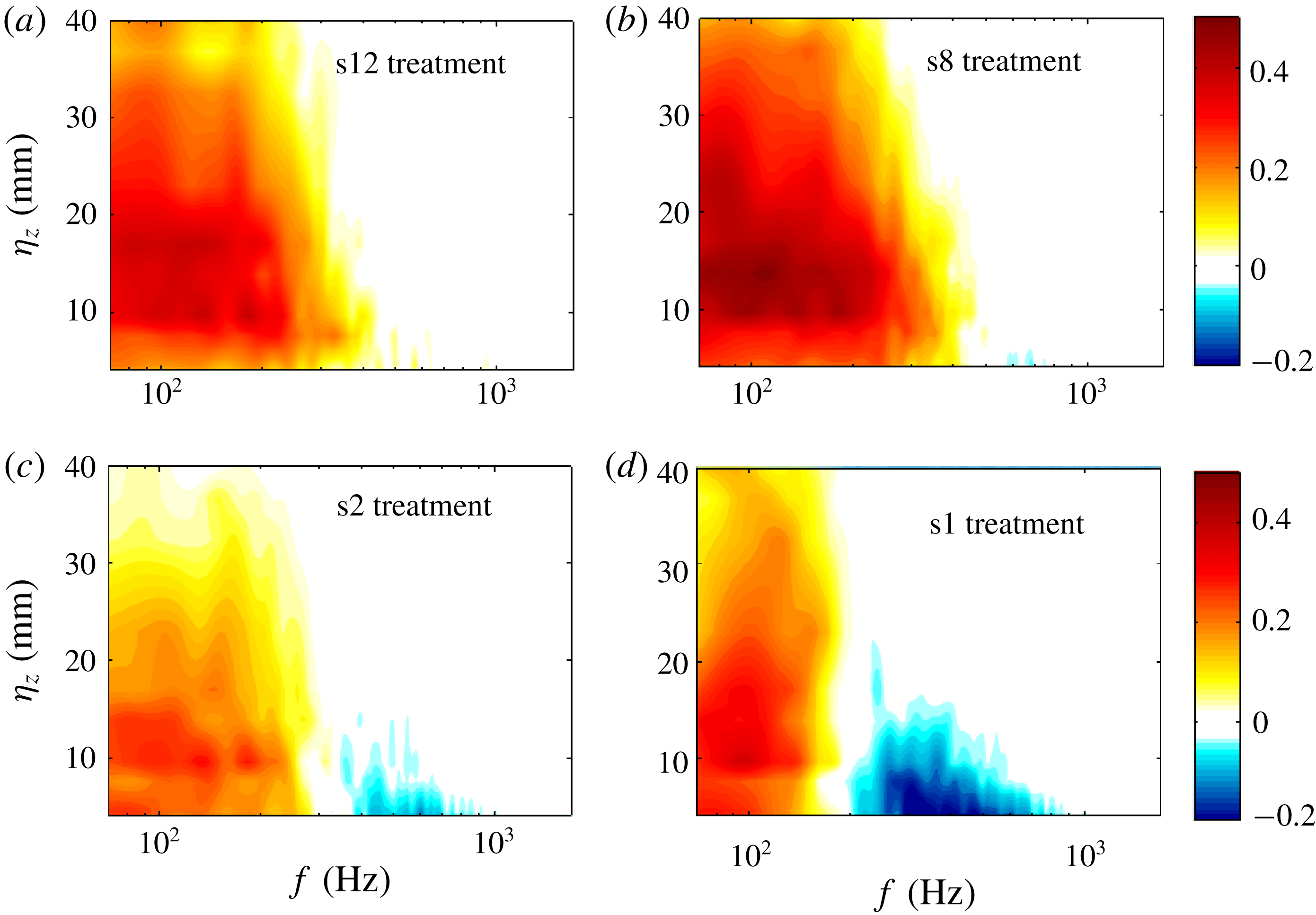
The effects of the finlet spacing on the lateral coherence of the boundary layer structures, measured using the spanwise microphones located at
 $x/c=0.976$
(
 $\bar{x}/h=8.6$
) are presented in figure 13. The results in this figure show the changes to the lateral coherence, i.e.
 $\unicode[STIX]{x0394}\unicode[STIX]{x1D6FE}^{2}=\unicode[STIX]{x1D6FE}_{treated}^{2}-\unicode[STIX]{x1D6FE}_{clean}^{2}$
, as a function of the separation distance (
 $\unicode[STIX]{x1D702}_{z}$
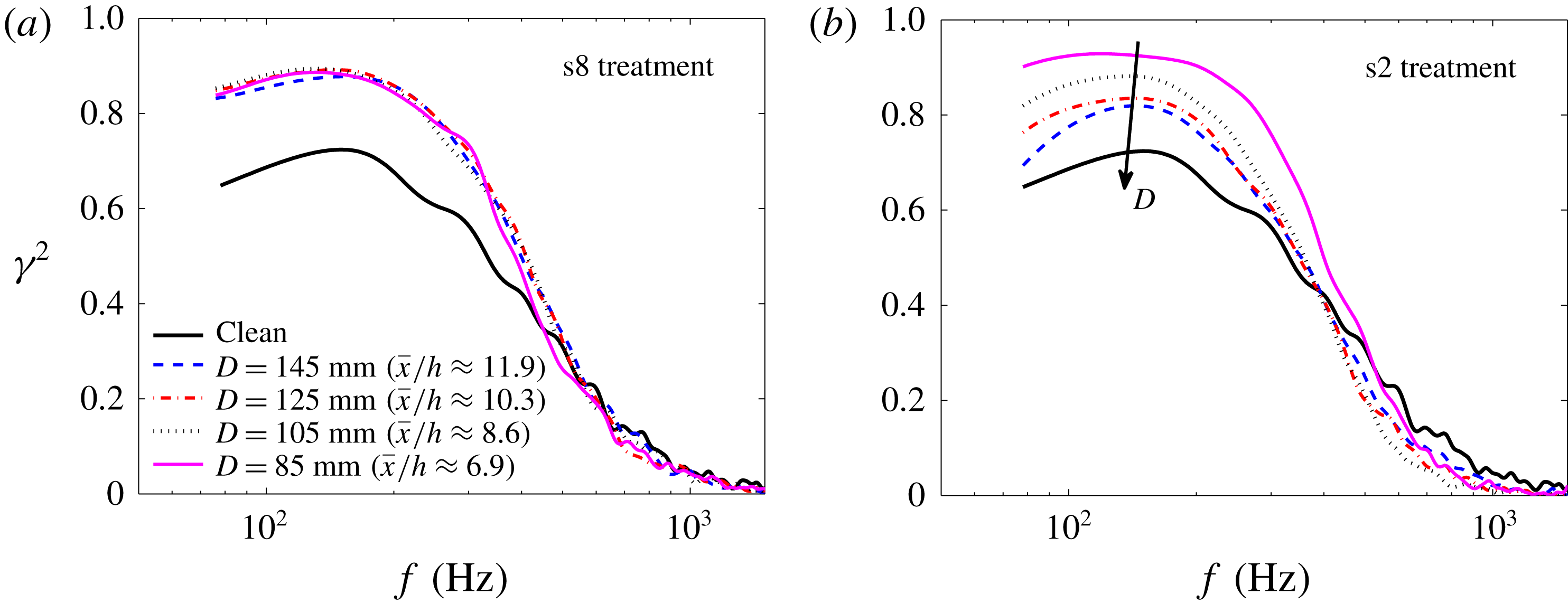
) and frequency. The lateral coherence results can provide some insight into the effects of the finlet treatment on the flow-field structures before reaching the plate trailing edge and generating noise. Consistent with our earlier observations, the results have shown again that the use of fine and coarse finlets can have very different effects on the spanwise coherence of the boundary layer structures. For the finlets with coarse spacing (s12 and s8), the presence of an upstream surface treatment leads to an increase in the lateral coherence at low to mid-frequencies without any significant changes to the coherence level at high frequencies (figure 13
a,b). The results for the finlets with fine spacing (s2), on the other hand, show that the finlets can significantly reduce the coherence at mid-frequencies. Despite the spanwise coherence reduction at mid-frequencies, the use of finely spaced finlets can result in an undesirable increase of coherence at low frequencies. By further reducing the spacing between the finlets (s1), these effects have been observed to intensify even further, i.e. more increase at low frequencies and more reduction at mid-frequencies.
Changes in the lateral coherence,
 $\unicode[STIX]{x0394}\unicode[STIX]{x1D6FE}^{2}=\unicode[STIX]{x1D6FE}_{treated}^{2}-\unicode[STIX]{x1D6FE}_{clean}^{2}$
, measured between spanwise microphones for different finlet treatments: (a) s12 treatment, (b) s8 treatment, (c) s2 treatment, (d) s1 treatment.

In addition to the trailing-edge surface pressure PSD studies, the frequency-dependent spanwise length scale and frequency-dependent convection velocity of the boundary layer structures in the trailing-edge region are among the important quantities for determining the far-field trailing-edge noise. The spanwise length scale of the surface pressure fluctuations,
 $\unicode[STIX]{x1D6EC}_{p,3}(f)$
, can be calculated using the spanwise coherence
 $\unicode[STIX]{x1D6FE}_{p,ij}^{2}(f)$
, measured using the p1 to p5 microphones at
 $x/c=0.976$
(thus
 $\unicode[STIX]{x1D6EC}_{p,3}(f)=\int _{0}^{\infty }\unicode[STIX]{x1D6FE}_{p,ij}(f,\unicode[STIX]{x1D702}_{z})\,\text{d}\unicode[STIX]{x1D702}_{z}$
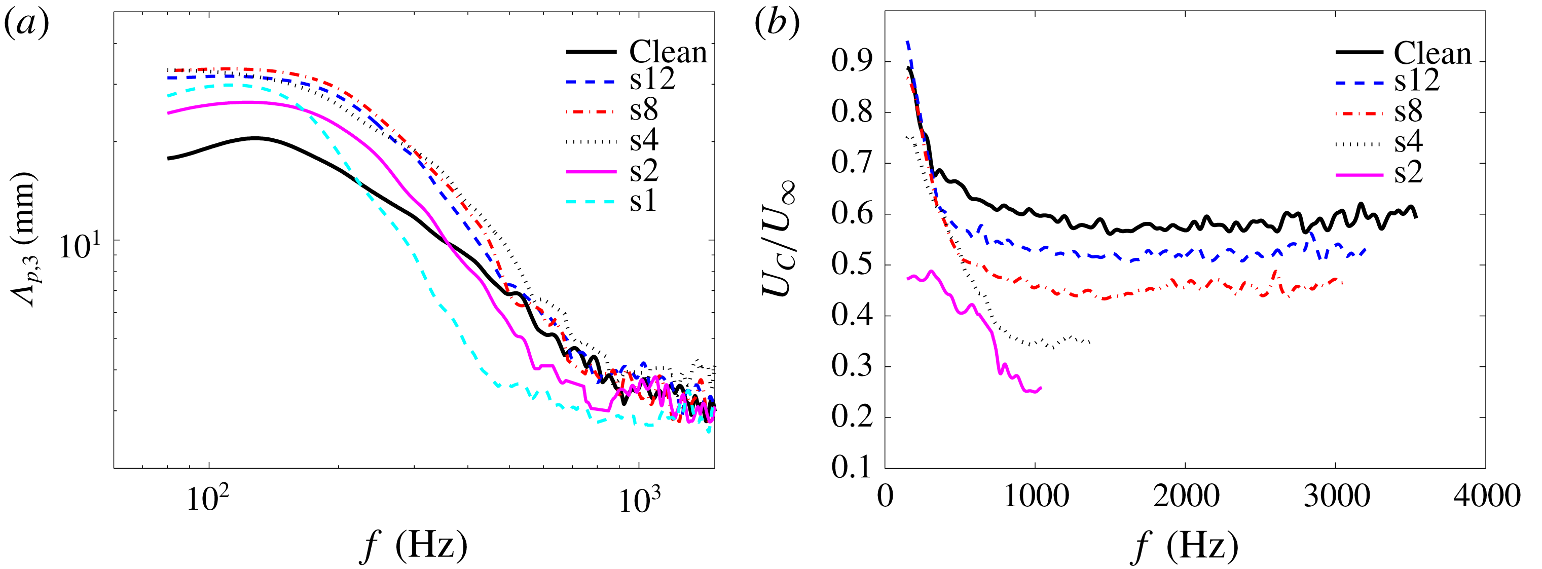
). Figure 14(a) shows the effects of the finlet spacing on the spanwise length scale. Similar to the lateral coherence data, the results here show that, for the case of coarse finlets, there is an increase in the spanwise length scale of the turbulent structures at low to mid-frequencies, up to approximately twice the value of the clean plate case, while no significant changes occur to the size of the structures at high frequencies. The results also show that, for the fine finlet spacings, the presence of an upstream surface treatment can significantly reduce the spanwise length scale at mid-frequencies and simultaneously increase it at low frequencies. Furthermore, by reducing the finlet spacing, the curves shift to lower frequencies. As can be seen, the maximum spanwise length scales for the s2 and s1 cases occur at approximately 130 Hz and 100 Hz, respectively, corresponding to
 $St=0.078$
and
 $0.06$
, which is also consistent with the PSD results observed in figure 8(b), indicating the shedding of large coherent structure within the wake of the finlet treatment. Therefore, the undesirable low-frequency increase in the spanwise length scale for the finlets with fine spacing is believed to be due to the shedding of large-scale vortical structures from the step introduced by the finlets, which is also in agreement with the results of previous studies for BFS geometries (Farabee & Casarella Reference Farabee and Casarella1986) and open BFS geometries (Liu et al.
Reference Liu, Ke, Chen and Sung2006).
(a) Spanwise length scale (
 $\unicode[STIX]{x1D6EC}_{p,3}$
) measured at
 $x/c=0.976$
. (b) Comparison of the eddy convection velocity between the clean and treated flat-plate cases.

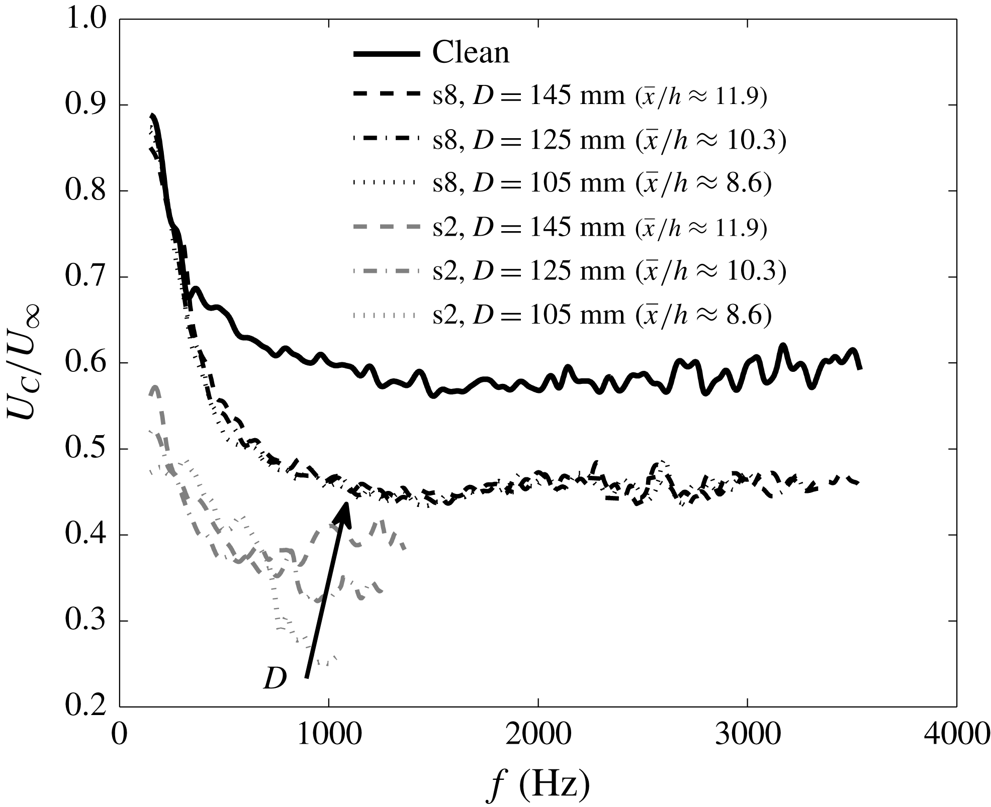
Figure 14(b) shows the frequency-dependent convection velocity of the turbulent eddies in the boundary layer, calculated using the phase analysis between the microphones p6 and p7 (
 $\unicode[STIX]{x1D702}_{x}=5.5~\text{mm}$
) near the trailing edge for the clean and treated flat plates, using the method described in § 3. The boundary layer convection velocity results are presented only for the configurations and frequency ranges with strong coherence between streamwise pressure transducers. The results for the clean plate show that at low frequencies (below 1000 Hz) the convection velocity is reduced as the frequency increases and reaches
 $U_{C}=0.6U_{\infty }$
and will then remain almost constant and independent of frequency. It is also clear from the results that the presence of the finlets leads to a reduction in the convection velocity of the boundary layer structures downstream of the surface treatment over the whole frequency range considered here. The convection velocity at very low frequencies, i.e. large structures, however, is less affected as a result of the use of the finlet treatments. Furthermore, it can be seen that reducing the finlet spacing causes more reduction of the convection velocity, particularly at mid- and high frequencies, which is consistent with the boundary layer mean velocity results (figure 11). As observed in figure 11, the velocity deficit experienced after the finlet treatments is more pronounced in the vicinity of the plate surface, where structures responsible for mid- to high frequencies are present. It can therefore be concluded from the results in figure 14(b) that the main effect of the finlets is felt by near-surface mid- to high-frequency structures.
4.5 Pressure–velocity correlation studies
To gain a better insight into the mechanisms through which finlets affect the boundary flow structures, the unsteady surface pressure and flow velocity are measured simultaneously. The pressure measurements are performed using the pressure transducers p1, p6, p8 and p9, at
 $\bar{x}/h=2.5$
, 4.8, 6.8 and 8.6, and the velocity measurements are carried out at various locations within the boundary layer above each pressure transducer. The space–time correlation of the surface pressure fluctuation and the velocity field,
 $R_{pu}$
, is defined here as
 $$\begin{eqnarray}R_{pu}(\bar{x},\bar{y},\unicode[STIX]{x1D70F})=\frac{\;\overline{p^{\prime }(\bar{x},t)u^{\prime }(\bar{x},\bar{y},t+\unicode[STIX]{x1D70F})}\,}{p_{rms}^{\prime }(\bar{x})u_{rms}^{\prime }(\bar{x},\bar{y})},\end{eqnarray}$$
where
 $p^{\prime }$
is the surface pressure fluctuation,
 $u^{\prime }$
is the streamwise fluctuating velocity fluctuation,
 $\unicode[STIX]{x1D70F}$
denotes the time delay between the signals and
 $\bar{y}$
is the vertical distance between the pressure transducer and the hot wire. By definition, a positive value of
 $\unicode[STIX]{x1D70F}$
indicates that the velocity signal lags the pressure signal. Furthermore, since the cross-spectrum is the Fourier transform of the cross-correlation, the cross-spectrum analysis can provide insight into the level of the contribution of different boundary layer structures to the pressure exerted on the surface at different frequencies. Thus, the coherence of the surface pressure fluctuations and velocity fluctuations, which is the normalized magnitude of the cross-spectrum, is employed here to quantify the influence of the local unsteady behaviour in the boundary layer on the exerted surface pressure field in the frequency domain. The coherence between the surface pressure and the streamwise velocity can be calculated as
 $$\begin{eqnarray}\unicode[STIX]{x1D6FE}_{pu}^{2}(\bar{x},\bar{y},f)=\frac{|\unicode[STIX]{x1D719}_{pu}(\bar{x},\bar{y},f)|^{2}}{\unicode[STIX]{x1D719}_{pp}(\bar{x},f)\unicode[STIX]{x1D719}_{uu}(\bar{x},\bar{y},f)},\end{eqnarray}$$
where
 $\unicode[STIX]{x1D719}_{pu}$
is the cross-spectrum between the pressure and velocity signals, and
 $\unicode[STIX]{x1D719}_{pp}$
and
 $\unicode[STIX]{x1D719}_{uu}$
are the autospectra of individual pressure and velocity signals, respectively.
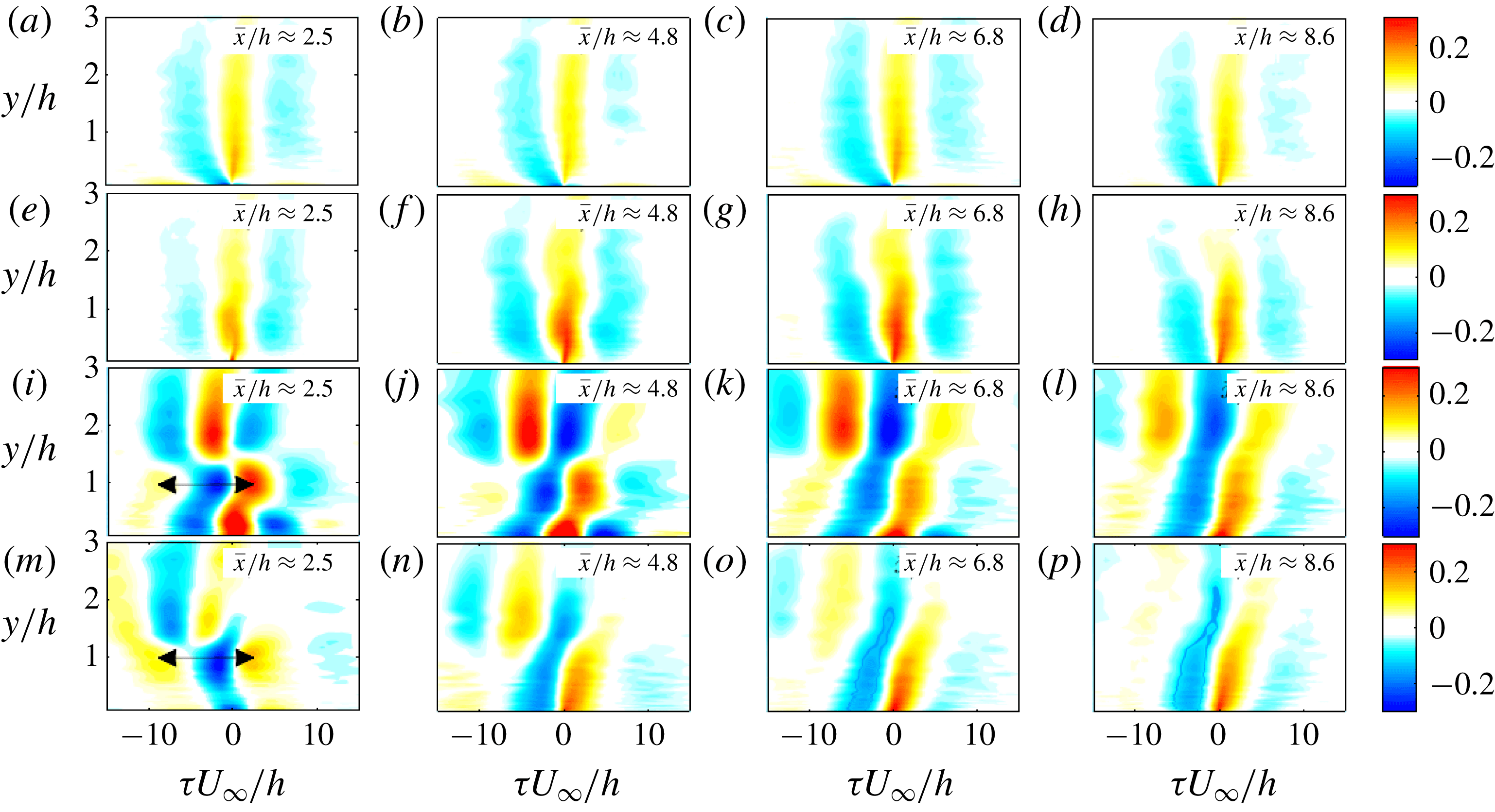
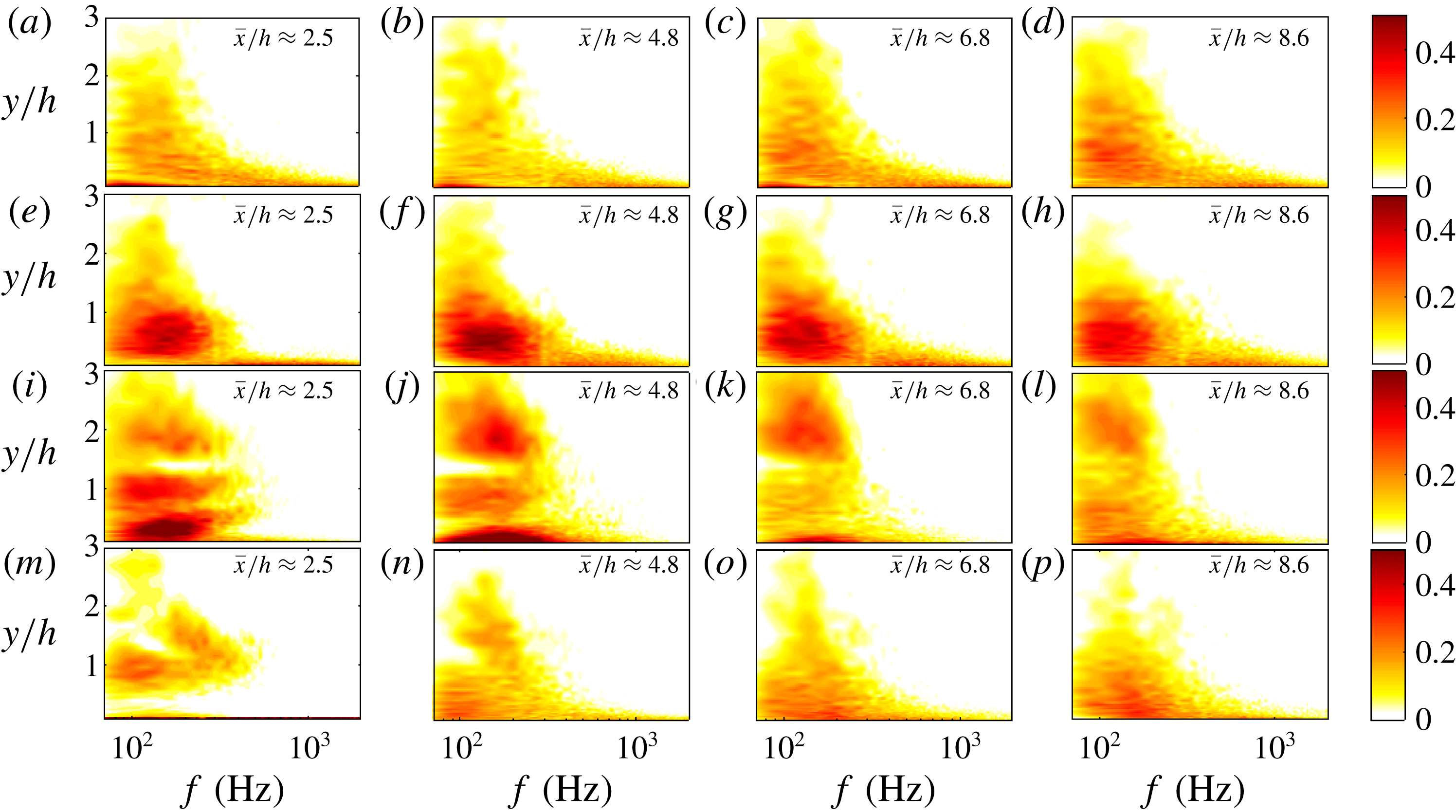
Temporal cross-correlation between the surface pressure fluctuations and boundary layer velocity (
 $R_{pu}$
) downstream of the surface treatments at several streamwise locations (
 $\bar{x}/h=2.5$
to 8.6) at
 $U_{\infty }=20~\text{m}~\text{s}^{-1}$
: (a–d) clean flat plate, (e–h) s8 treatment, (i–l) s2 treatment, (m–p) s0 BFS.

The contour plots of the temporal cross-correlation between
 $p^{\prime }$
and
 $u^{\prime }$
at several streamwise locations (
 $\bar{x}/h=2.5$
to 8.6) downstream of the finlet treatments are presented in figure 15. The results of the clean flat plate are also provided for comparison. As can be seen, for the clean flat plate a definite cross-correlation due to the different scales in the turbulent boundary layer can be observed at all streamwise positions. This correlation behaviour for the clean plate can be characterized by distinct positive and negative correlation islands that extend up to at least half the boundary layer thickness (equivalent to
 $3h$
in the plots) from the surface of the plate (Naka et al.
Reference Naka, Stanislas, Foucaut, Coudert, Laval and Obi2015). This is an indication of the presence of large structures with long lifespan that maintain their coherence over long distances. Furthermore, the highest correlation occurs in the positive range of the non-dimensional time delay
 $(\unicode[STIX]{x1D70F}U_{\infty }/h)$
, indicating that the surface pressure fluctuations have the strongest correlation with the upstream turbulence structures and that the upstream turbulence structures play an important role in the generation of the surface pressure fluctuations. The cross-correlation pattern for the coarse finlets (s8) shows a very similar trend to that of the clean flat plate. The main effect of the coarse finlets, however, is the increase in the magnitude and size of the correlation islands at the near-wall region (
 $y/h<1.5$
), suggesting the presence of turbulence structures with a longer lifespan. Similar to the results of the clean flat plate, the correlation results do not change greatly within
 $\bar{x}/h=2.5$
to 8.6.
The pressure–velocity correlation results for the s2 finlets reveals a much more complex flow field. Unlike the flat plate and coarse finlets, the pressure–velocity correlation results change greatly from the near-wake region of the finlets (
 $\bar{x}/h=2.5$
), where three different high-correlation areas with the boundary layer can be observed, to further downstream (
 $\bar{x}/h=8.6$
), where results show a strong resemblance to that of a BFS (figure 15
o, p). At
 $\bar{x}/h=2.5$
(figure 15
i), three different areas of strong
 $p$
–
 $u$
correlation have can be readily identified. The three regions of high pressure–velocity correlation are as follows: (i) an area of high
 $p$
–
 $u$
correlation near the wall (
 $y/h<1$
), i.e. below the finlet shear layer, which is absent in the BFS case (figure 15
m), showing the contribution of the finlet discharge flow to the surface pressure fluctuations. (ii) A quasi-periodic structure at
 $y/h\approx 1$
, i.e. the step height. A similar result can also be seen in the case of the BFS configuration. Owing to the fact that the shedding of large-scale vortical structures above the wall induces a negative peak above the pressure sensor (Kiya & Sasaki Reference Kiya and Sasaki1983; Cherry, Hillier & Latour Reference Cherry, Hillier and Latour1984), this high
 $p$
–
 $u$
correlation area is believed to be indicative of the presence of vortical shedding structures, originating from the upper surface of the finlets (
 $y/h\approx 1$
). As can be seen, the value of the non-dimensional time delay
 $\unicode[STIX]{x1D70F}U_{\infty }/h$
(between two maxima or minima, indicated as
 $\unicode[STIX]{x1D70F}$
in the figures), related to the periodicity of this quasi-periodic vortex shedding, is approximately 12, corresponding to the frequency of 138 Hz, which is in agreement with the centre frequency of the broadband peak in the surface pressure PSD in figure 8. (iii) Finally, an area of strong correlation away from the wall, within
 $1.3<y/h<3$
. Progressing downstream, the high-correlation areas (at
 $y/h\approx 1$
) become wider, as a result of the vortex coalescence mechanism, formation of larger structures and energy shift to lower frequency (Winant & Browand Reference Winant and Browand1974), as also observed in figure 12. Furthermore, while for the coarse finlet treatment (s8), the correlation decays quickly with
 $y/h$
and becomes insignificant for the locations
 $y/h>1$
, similar to the clean flat plate, in the case of the fine finlets (s2) and the BFS cases, the pressure–velocity correlation extends up to approximately
 $y/h=3$
, due to the separation of the flow and the emergence of large-scale vortical structures behind the finlets. These observations corroborate the conclusions drawn previously in § 4.3 that the dominant mechanism for the generation of the surface pressure fluctuations in the case of fine finlet treatments is the separated shear layer, while for the coarse finlets, the turbulence structures in the boundary layer play the most important role.
Coherence between the surface pressure and boundary layer velocity fluctuations (
 $\unicode[STIX]{x1D6FE}_{pu}^{2}$
) downstream of the surface treatments at several streamwise locations (
 $\bar{x}/h=2.5$
to 8.6): (a–d) clean flat plate, (e–h) s8 treatment, (i–l) s2 treatment, (m–p) s0 BFS.

Figure 16 shows the contour plots of coherence between the surface pressure and velocity fluctuations (
 $\unicode[STIX]{x1D6FE}_{pu}^{2}$
) at several streamwise locations downstream of the finlets between
 $\bar{x}/h=2.5$
and 8.6. The results of the clean flat-plate and the BFS cases are also provided for comparison. As can be seen, for the clean flat plate, the
 $p$
–
 $u$
coherence decreases with the vertical distance (
 $y/h$
) and frequency at all streamwise locations. The broadband coherence peak occurring at
 $f\approx 120~\text{Hz}$
and
 $y/h\approx 0.6$
coincides with the surface pressure spectral peak found for the clean flat plate in figure 8. In the case of a coarse finlet treatment (s8), an area of increased coherence can be observed within the frequency range of
 $80~\text{Hz}<f<400~\text{Hz}$
and the wall distance of
 $0<y/h<1.5$
. This behaviour, along with the cross-correlation contour maps in figure 15, shows the effect of coarse finlets and the emergence of a highly coherent structure downstream of the finlets as a result of the channelling of the boundary layer flow between the finlets. The results have also shown that these newly formed structures retain their coherence over a long distance after the finlet treatment.
In the case of the s2 finlet treatment, the finlets are shown to split up the
 $p$
–
 $u$
coherence contour map into three regions in the wall-normal direction. In addition to the cross-correlation observations in figure 15(i) for these three areas, the results here can also provide some interesting information about the frequency content of each area. Compared to the clean flat-plate and the BFS cases, in the case of the s2 finlet treatment, a new area of increased
 $p$
–
 $u$
coherence at low frequencies and within
 $0<y/h<0.6$
is observed. Such behaviour cannot be seen in the BFS results and can therefore only be attributed to the low-momentum flow discharged through the finlet channels into the wake region of the finlets. It can also be seen that this area of high coherence widens in the frequency domain, moves closer to the wall surface and loses its coherence at further downstream locations. The second high coherence region occurring at around
 $y/h\approx 1$
, also seen in the BFS case, is due to the quasi-periodic vortex shedding from the finlet upper surface (see figure 15
i). The maximum coherence,
 $\unicode[STIX]{x1D6FE}_{pu}^{2}$
, at this region appears at approximately
 $f=100{-}150~\text{Hz}$
, which is consistent with the frequency of the spectral peak in the surface pressure PSD and lateral coherence results presented in figures 8 and 14, respectively. Far away from the wall, at
 $y/h\approx 2$
, there is a third high
 $p$
–
 $u$
coherence region, which was also seen in the cross-correlation maps in the form of negative and positive correlation islands. This region of high coherence away from the surface is attributed to the external irrotational flow, as previously observed by Lee & Sung (Reference Lee and Sung2002). Furthermore, the results show that the use of fine finlets (s2) can reduce the pressure–velocity coherence at mid- to high frequencies, which is in agreement with the lateral coherence results presented in figures 13 and 14. Finally, the comparison of the flow patterns observed for the s8 and s2 finlets also suggests that the lifespan of the structures formed due to the interaction of the boundary layer with the s2 finlets is much shorter than those downstream of the s8 finlets, and go through severe changes as they travel downstream.
4.6 Optimum finlet spacing
The results presented in the previous sections have demonstrated that the flow field downstream of the finlet treatments has a complex nature and is strongly dependent on the finlet spacing. Depending on the finlet spacing, the treatment can exhibit boundary channelling effects or appear like a BFS. The effectiveness of the treatment for the reduction of the surface pressure fluctuations with minimum low-frequency noise increase penalty was also found to be directly related to the ability of the finlets to channel the flow and reduce the energy content of the boundary layer structures. The low-frequency noise increase, similar to the BFS cases, was shown to be related to the flow separation from the top surface of the treatment and the generation of a strong shear layer.
Based on our observations in § 4.1, the surface pressure PSD variation is not a monotonic function of the finlet spacing (
 $s$
) and, while reducing the spacing between the finlets improves the efficiency of the coarse finlets in reducing the surface pressure PSD, for the finlets with fine spacing it causes an undesirable low-frequency surface pressure PSD increase. Therefore, to achieve maximum surface pressure PSD reduction, the spacing between the finlets should be sized such that, while the wetted surface area is maximized, the formation of the shear layer caused by the flow passing over the surface treatment is prevented. To obtain the optimum finlet spacing, the pressure PSD contour plot, normalized by the results of the clean flat-plate case (
 $\unicode[STIX]{x0394}\unicode[STIX]{x1D719}_{pp}=10\log _{10}(\unicode[STIX]{x1D719}_{pp,treated}/\unicode[STIX]{x1D719}_{pp,clean})$
), measured by microphone p1 (
 $x/c=0.976$
or
 $\bar{x}/h=8.6$
) at
 $U_{\infty }=20~\text{m}~\text{s}^{-1}$
, is presented in figure 17. As can be seen, there is an optimum finlet spacing that satisfies the above-mentioned requirements and it is somewhere around 4 mm for the cases considered in this study. Furthermore, the pressure PSD contour plot shows that the maximum reduction in the surface pressure PSD was achieved within the frequency range of
 $f=4{-}7~\text{kHz}$
. This behaviour is very similar to that observed by Clark et al. (Reference Clark, Daly, Devenport, Alexander, Peake, Jaworski and Glegg2016) for fibre canopies suspended above a surface.
Normalized surface pressure PSD,
 $\unicode[STIX]{x0394}\unicode[STIX]{x1D719}_{pp}=10\log _{10}(\unicode[STIX]{x1D719}_{pp,treated}/\unicode[STIX]{x1D719}_{pp,clean})$
, contour plot for finlets with different spacing (
 $s$
) measured at
 $x/c=0.976$
.

To obtain a more global criterion for the optimum finlet spacing as a function of the boundary layer thickness, various experiments have been conducted using the finlets listed in § 2.4, placed in flows with various boundary layer thicknesses. To achieve different boundary layer thickness, the flow over the flat-plate test rig was tripped using different methods. All boundary layer cases have been assessed and validated using the approach described in § 3. In figure 18(a), the surface pressure PSD results for the treated flat plate, normalized by the results of the clean flat-plate case (
 $\unicode[STIX]{x0394}\unicode[STIX]{x1D719}_{pp}=10\log _{10}(\unicode[STIX]{x1D719}_{pp,treated}/\unicode[STIX]{x1D719}_{pp,clean})$
) are presented for several boundary layer thicknesses and finlet treatment spacings. The analysis has been carried out for different frequencies, but the results are presented for only
 $f=5~\text{kHz}$
, where maximum reduction in surface pressure PSD was previously achieved (see figure 17). The results in figure 18(a) show that the optimum finlet spacing (
 $s$
) shifts to higher values as the boundary layer thickness to finlet height ratio (
 $\unicode[STIX]{x1D6FF}/h$
) increases and that the amount of the PSD reduction for the finlets with fine spacing decreases with
 $\unicode[STIX]{x1D6FF}/h$
. For the coarse finlet cases (s8 and s12), little variation has been seen as
 $\unicode[STIX]{x1D6FF}/h$
varies, indicating that the effectiveness of the coarse finlets in reducing the surface pressure PSD is nearly independent of the boundary layer thickness. As one would expect, by increasing the boundary layer thickness, there will be space for larger turbulence structures and therefore larger finlet spacing will be required for capturing and channelling of such structures through the finlets. This can also be interpreted as there being a minimum finlet spacing criterion for capturing large turbulence structures in the boundary layer. In figure 18(b), the same data as in figure 18(a) are presented while the
 $x$
-axis is normalized by the boundary layer thickness (
 $s/\unicode[STIX]{x1D6FF}$
) and the
 $y$
-axis shows
 $\unicode[STIX]{x0394}\unicode[STIX]{x1D719}_{pp}\unicode[STIX]{x1D6FF}/h$
, where
 $h$
is the height of the finlets. It can be seen that the data for finlets with fine spacing collapse almost onto a single curve, showing that the efficiency of the finely spaced finlets in reducing the surface pressure PSD is a function of
 $\unicode[STIX]{x1D6FF}/h$
and the optimum finlet spacing occurs at
 $s\approx 0.07\unicode[STIX]{x1D6FF}$
. Therefore, to achieve maximum reduction in the surface pressure PSD with minimum increase in the low to mid-frequencies, the spacing between the finlets should be of the order of the size of the boundary layer inner layer (
 $y/\unicode[STIX]{x1D6FF}\approx 0.1$
) (Pope Reference Pope2001).
Normalized surface pressure PSD plots,
 $\unicode[STIX]{x0394}\unicode[STIX]{x1D719}_{pp}=10\log _{10}(\unicode[STIX]{x1D719}_{pp,treated}/\unicode[STIX]{x1D719}_{pp,clean})$
, as a function of the finlet spacing (
 $s$
), at
 $f=5~\text{kHz}$
, measured at
 $x/c=0.976$
.

4.7 Effect of finlet distance from the trailing edge
The streamwise distance of the finlets from the trailing edge (
 $D$
) can change the flow field and the level of surface pressure fluctuation reduction. To better understand the effect of the finlet distance from the trailing edge, tests have been carried out using the s8 and s2 finlets positioned at different streamwise distances from the trailing edge, namely
 $D=145$
, 125, 105, 85 and 65 mm upstream of the trailing edge, corresponding to roughly 75 %, 78 %, 82 %, 85 % and 89 % of the chord, as shown in figure 4.
The effects of finlet distance from the trailing edge on the surface pressure PSD measured using the trailing-edge microphone (p1, at
 $x/c=0.976$
) at
 $U_{\infty }=20~\text{m}~\text{s}^{-1}$
are presented in figure 19(a,b) for the s2 and s8 finlet cases, respectively. As can be seen, the two finlets show a very different behaviour. For the coarse finlets (s8), changing the streamwise position of the surface treatment relative to the trailing edge has almost no effect on the PSD behaviour and the surface pressure spectra remain nearly unchanged. This is consistent with the velocity PSD contour results at different streamwise locations behind the finlets (figure 12), and corresponding boundary layer mean velocity and turbulent intensity profiles (figure 11) and shows that the overall structure of the boundary layer remains unaltered downstream of coarse finlets. On the other hand, for the dense finlets (s2), the streamwise location of the finlets seems to affect only the decay rate at high frequencies, while the low-frequency peak remains essentially unchanged, in terms of both its amplitude and frequency. The low-frequency peak in the case of the s2 finlets occurs at approximately 130 Hz, corresponding to the Strouhal number of 0.078, and is over 10 dB higher than that of the clean flat plate. As explained previously, the low-frequency increase in the surface pressure PSD in the case of dense finlets is due to the low-frequency shear layer structures originating from the top surface of the finlets (see figure 12). As shown in figure 19(b), moving the s2 finlets towards the trailing edge leads to more reduction in the surface pressure PSD at mid- to high frequencies, similar to the observations in the literature for the cases of flow behind a BFS (Farabee & Casarella Reference Farabee and Casarella1986; Ji & Wang Reference Ji and Wang2012). Finally, it can be concluded that, while the efficiency of the coarse finlet treatments in reducing the surface pressure PSD is nearly independent of their streamwise position, in the case of dense finlets, the mid- to high-frequency performance of the treatment can be improved by positioning it closer to the trailing edge.
The effect of finlet distance from the trailing edge on the surface pressure PSD at
 $x/c=0.976$
: (a) s8 finlet treatment and (b) s2 finlet treatment.

The effects of the finlet distance from the trailing edge on the lateral coherence of the boundary layer structures for the coarse and dense finlet treatments at different streamwise distances from the trailing edge are presented in figure 20. The results are presented only for a single pressure sensor separation distance of
 $\unicode[STIX]{x1D702}_{z}=3.2~\text{mm}$
. The results have again shown that the two finlet treatments have very different effects on the boundary layer flow. For the finlets with coarse spacing (s8), changing the streamwise position of the surface treatment causes no major changes to the structure of the boundary layer and the downstream lateral coherence remains nearly unchanged (figure 20
a), similar to the PSD results in figure 8(a). The results for the dense finlets (s2), on the other hand, show that moving the finlets closer to the trailing edge can lead to an increase in the lateral coherence of the boundary layer structures at low frequencies and a slight reduction at high frequencies (see figure 20
b). This also shows that the shear layer of the s2 finlet case, responsible for significant changes in the pressure–velocity correlations, undergoes a relaxation process with distance, which is a characteristic feature of BFS flows (Bradshaw & Wong Reference Bradshaw and Wong1972).
Effects of the streamwise distance of the finlet treatments on the lateral coherence (
 $\unicode[STIX]{x1D6FE}^{2}$
) measured between two spanwise microphones with a lateral distance of
 $\unicode[STIX]{x1D702}_{z}=3.2~\text{mm}$
: (a) s8 finlet treatment and (b) s2 finlet treatment.

Lastly, the effects of the streamwise distance of the finlets from the trailing edge on the convection velocity of the turbulent eddies in the boundary layer, calculated using the data collected by microphones p6 and p7 (
 $\unicode[STIX]{x1D702}_{x}=5.5~\text{mm}$
) near the trailing edge at
 $20~\text{m}~\text{s}^{-1}$
, are presented in figure 21. As before, the convection velocity results are provided only for the cases and frequency ranges with strong coherence between streamwise pressure transducers. The results for the coarse finlet case (s8) show that the boundary layer structures convection velocity does not change greatly by moving the finlets closer to the trailing edge, which is consistent with the pressure spectra (figure 19
a and lateral coherence results figure 20
a). This indicates that, while the mid- and high-frequency energy content of the boundary layer can be greatly changed, moving coarse surface treatments towards the trailing edge has no noticeable effect on the overall structure of the boundary layer. For the finlets with dense spacing (s2), however, moving the finlet treatment towards the trailing edge causes significant reduction in the convection velocity. This also agrees well with the observations of Farabee & Casarella (Reference Farabee and Casarella1986) for a BFS.
Eddy convection velocity for a clean flat plate and flat plate with finlet treatments at different streamwise distances from the trailing edge (
 $D$
).

5 Conclusions
The present study is concerned with the experimental investigation of surface treatments as a means of passive trailing-edge noise control. The effects of upstream streamwise finlets, the spacing between the finlets and the finlet distance from the trailing edge on mean surface pressure distribution, surface pressure spectra, eddy convection velocity and spanwise length scale have been experimentally investigated using a long flat-plate model. Furthermore, velocity measurements downstream of the finlets and the simultaneously measured unsteady velocity and surface pressure data have provided further information about the trailing-edge flow field and the potential noise reduction mechanisms. The results have revealed that the flow behaviour downstream of the finlets can be strongly affected by the spacing between the finlets. In the case of finlet treatments with coarse spacing, a reduction in the surface pressure PSD at mid- to high frequencies and an increase in the spanwise length scale has been observed. It is hypothesized that for the finlets with coarse spacing, the boundary layer coherent turbulent structures are channelled and travel through the finlets and therefore their energy can be dissipated through friction with the walls. In these cases, reducing the spacing between the finlets leads to an increase in the wetted surface area and therefore more reduction in the downstream surface pressure spectra. On the other hand, for the case of finlets with fine spacing, the high-frequency pressure spectra can be reduced significantly, but with an undesirable low- to mid-frequency elevation. It is hypothesized that, for the finlets with fine spacing, some portions of the upstream flow separates at the end corner of the finlets and forms a free shear layer, similar to the flow over a BFS. This region with high-energy structures gives rise to a low-frequency increase in the pressure PSD. Furthermore, the finlets can significantly reduce the spanwise coherence of the boundary layer structures at mid- to high frequencies. The eddy convection velocity is also observed to reduce downstream of all finlet spacing and the reduction increases with reducing the spacing between the finlets. The performance of the finlets for reducing the surface pressure PSD is found to be dependent on the finlet spacing. The results have shown that maximum pressure PSD reduction can be achieved when the finlet spacing is approximately
 $0.07\unicode[STIX]{x1D6FF}$
.
The static mean surface pressure distribution has revealed that, while the finlet treatments with coarse spacing induce a low level of pressure gradient downstream of the surface treatment area, reducing the spacing between finlets leads to the emergence of an APG region behind the finlets. The mean velocity and turbulence intensity profiles measured downstream of the surface treatments showed that in all cases a significant velocity deficit occurs downstream of the finlets, accompanied by a reduced turbulence intensity near the wall. However, by reducing the finlet spacing, an increase in the turbulence intensity at around
 $y/h\approx 1$
appears, which is the shear layer of the surface treatment. It was then concluded that, while less permeable finlets may cause a greater reduction in the boundary layer mean velocity, the greater turbulence in its wake will make the treatment less effective for unsteady surface pressure reduction than a more permeable one. Furthermore, the velocity PSD results show that, for the cases with fine spacing, the flow separation behind the treatment and the emergence of the high-energy content region at
 $0.5<y/h<2$
are responsible for the undesirable low-frequency energy increase and also reducing the finlet effectiveness at high frequencies. One can, therefore, conclude that the finlets wake region is characterized by the interaction between a lower layer of relatively low-velocity wind and a region of higher-velocity wind flowing above the finlets. Because of the finite porosity of the finlets, the structure of turbulence downstream of the finlets experiences both flow types and therefore it can be said that the flow behind the finlets is a superposition of channel flow exiting the finlets and the BFS flow, with their relative importance determined by the finlet spacing. The pressure–velocity correlation results showed that, while the main effect of the coarse finlets is to increase the magnitude and size of the correlation islands at the near-wall region (
 $y/h<1.5$
), suggesting the presence of turbulence structures with a longer lifespan with respect to the clean case as a result of the flow channelling between the finlets, for the fine finlets there exists a much more complex flow field downstream of the finlets. The dominant mechanism for the generation of the surface pressure fluctuations in the case of fine finlet treatments is the separated shear layer. Furthermore, the
 $p$
–
 $u$
coherence results suggest that the lifespan of the structures formed due to the interaction of the boundary layer with the fine finlets is much shorter than those downstream of the coarse finlets, and go through severe changes as they travel downstream. The results also show that, while the efficiency of the finlet treatments with coarse spacing in reducing the surface pressure PSD, the lateral coherence and the eddy convection velocity is almost independent of the streamwise position of the treatment, the efficiency of the fine finlets changes significantly with the distance from the trailing edge.
Acknowledgement
The second author (M.A.) would like to acknowledge the financial support of the Royal Academy of Engineering.