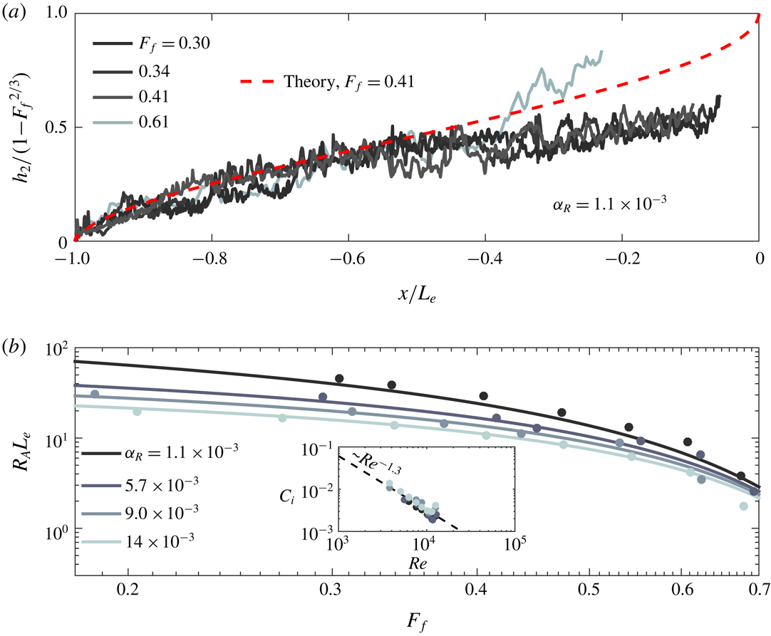
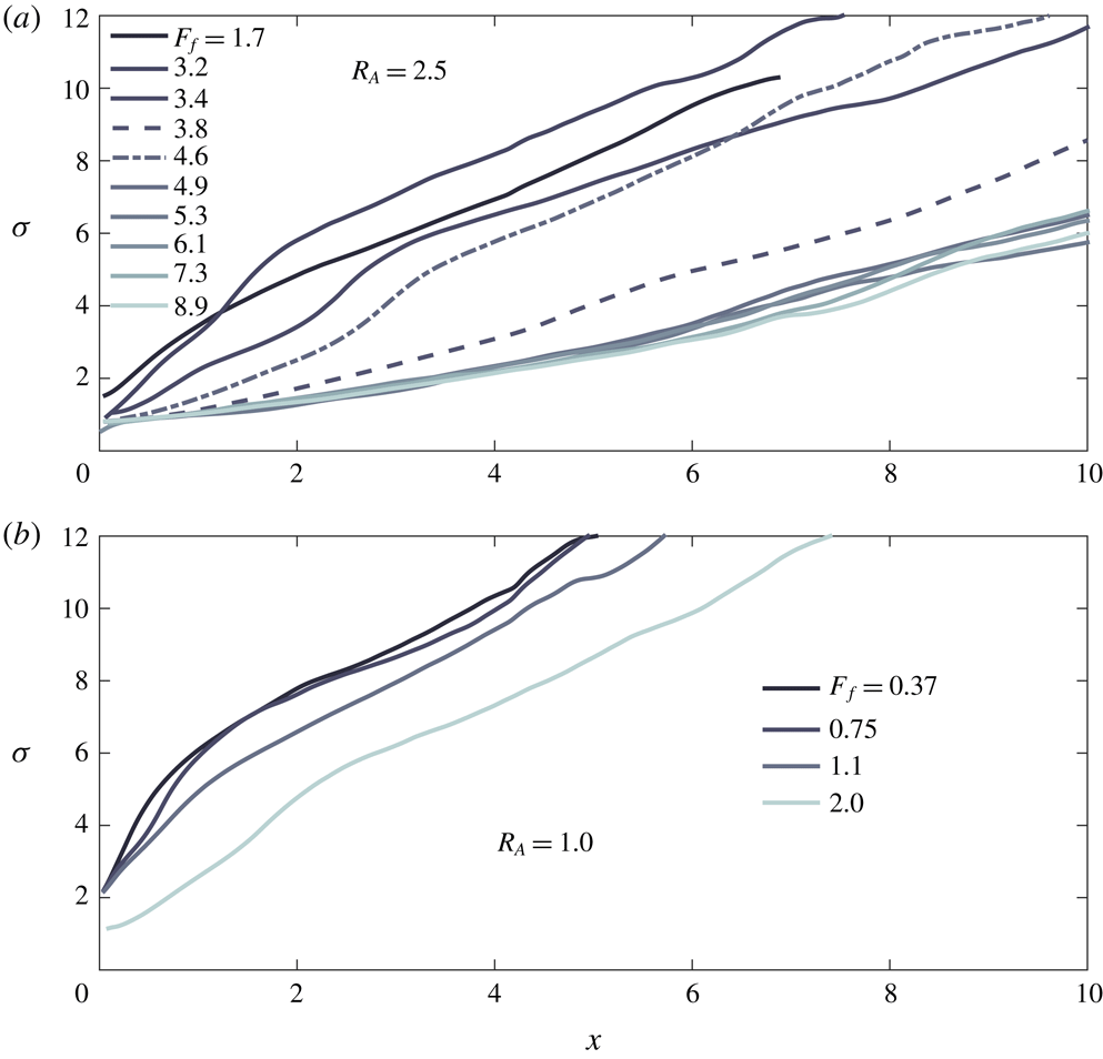
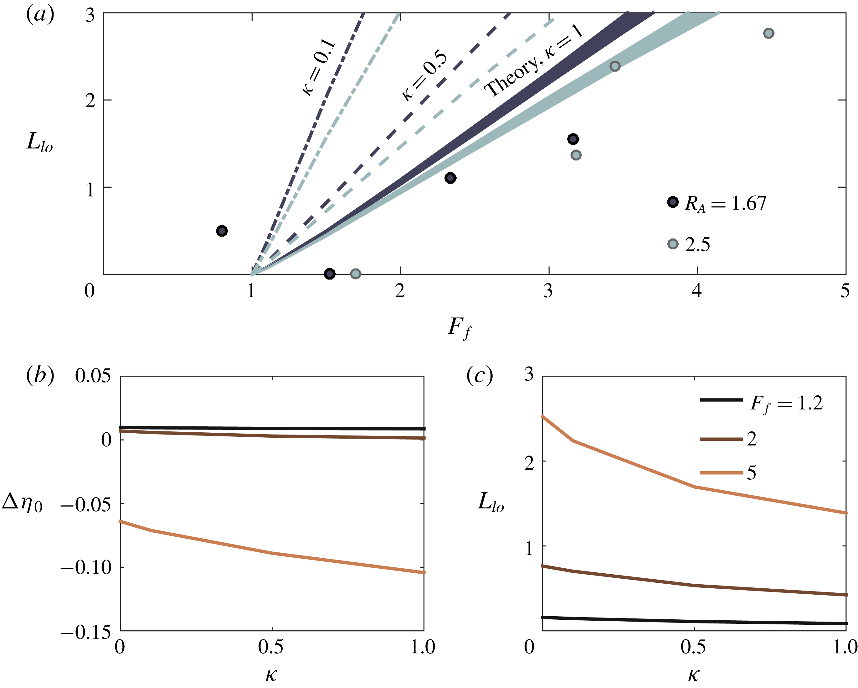
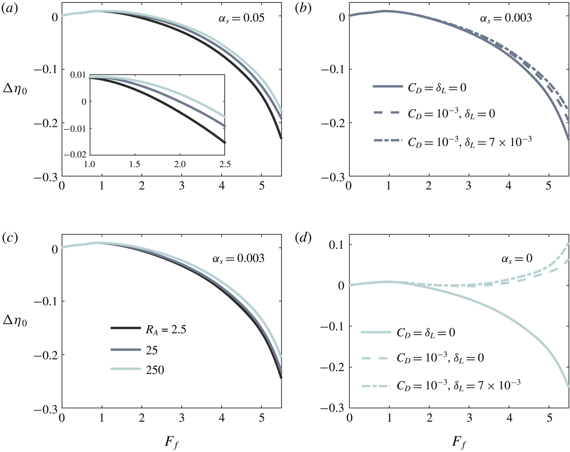
1 Introduction
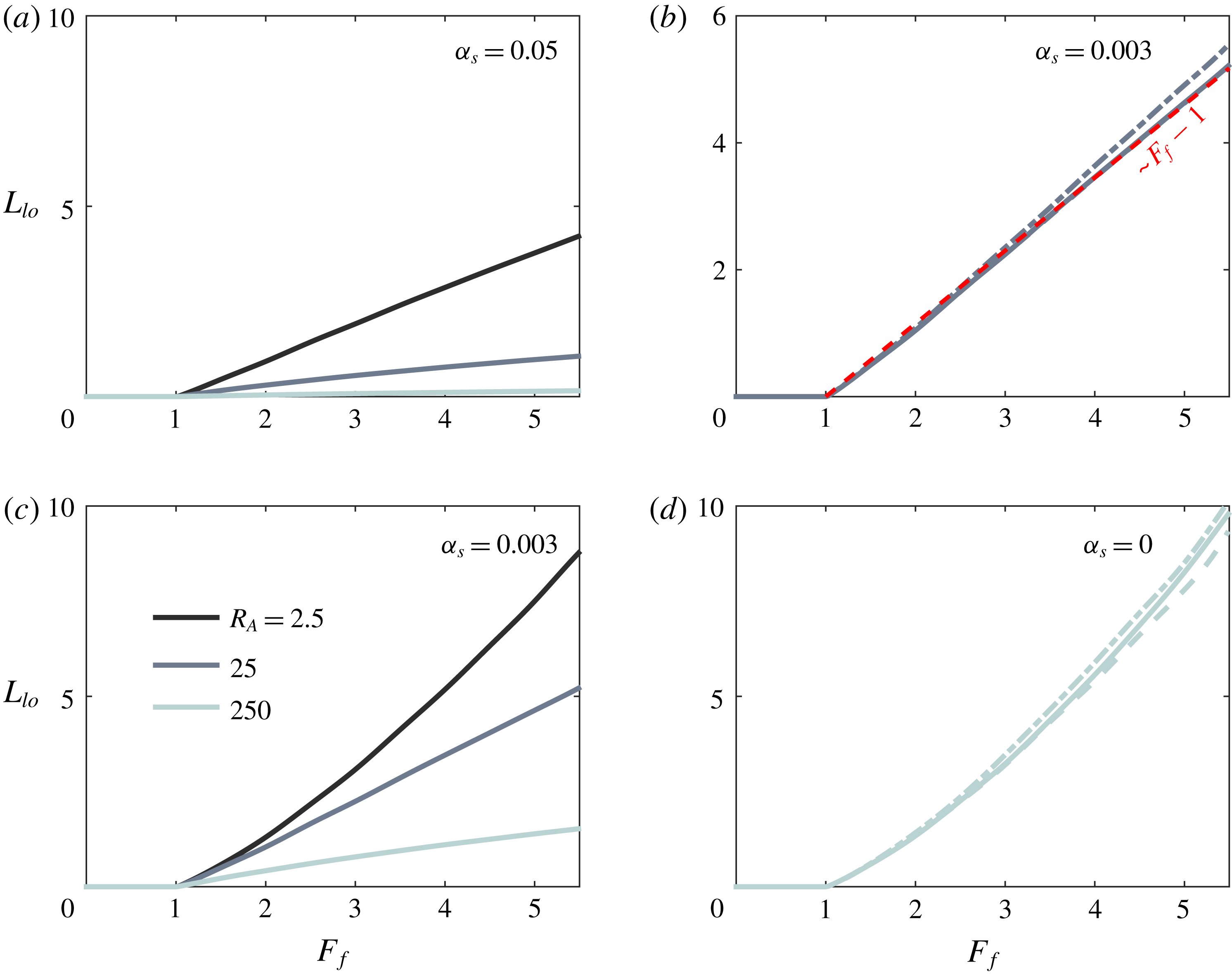
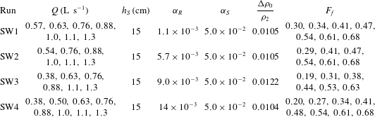
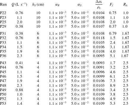
Rivers act as conduits of terrestrially derived nutrients, contaminants, biological material and sediment to the coastal ocean. Delivery to the coastal ocean is mediated by complex circulation patterns in the lower river, estuary and river plume, hereafter termed the river–ocean interface. Circulation in this region is driven by the interplay of a variety of forcing mechanisms, among them the barotropic forcing of the river and tides and the baroclinic forcing engendered by the contrast in salinity between the river and ambient coastal water. In the case of strongly stratified estuarine and plume systems, one of the principal dynamic features of the river–ocean interface is the detachment of the buoyant outflowing water from the channel bed or sea floor. This mechanism is of particular importance to the transport of sediment; bottom detachment (hereafter referred to as liftoff) results in the reduction of bed stress and thus particle resuspension rates (Fugate & Chant Reference Fugate and Chant2005) as well as the reduction of turbulence intensity and consequently the turbulent particle suspension capacity in the outflowing buoyant layer (Kostaschuk, Church & Luternauer Reference Kostaschuk, Church and Luternauer1992; Geyer Reference Geyer1993). Additionally, mixing of fluvial and ambient coastal water begins at liftoff; mixing between the water masses modifies the salinity in the outflowing layer, engendering flocculation and thus enhanced deposition rates for fine sediments (e.g. Geyer, Hill & Kineke Reference Geyer, Hill and Kineke2004).
The structure of the plume forming directly offshore of the river mouth is also determined by the location of liftoff, in particular whether it is within the river (low discharge) or is pushed into the coastal ocean (high discharge). The formation of subaqueous canyons via the deposition of fluvial sediment in the coastal ocean is understood to be a crucial mechanism in delta progradation (Jerolmack Reference Jerolmack2009). However, this mechanism is predicated on the formation of a rapidly depositional bottom-attached and decelerating plume, in contrast to the initially accelerating, surface-trapped plume typically discussed in the plume literature (e.g. Hetland Reference Hetland2010; Kilcher & Nash Reference Kilcher and Nash2010; Horner-Devine, Hetland & MacDonald Reference Horner-Devine, Hetland and MacDonald2015). Understanding under what conditions and to what extent liftoff can be forced offshore is a crucial step in better understanding the morphodynamic processes responsible for delta growth and evolution.
The structure of the free-surface elevation profile is also important for sediment transport and morphodynamics in the river–ocean interface. Far upstream of the mouth, the river adjusts to a uniform depth characterized by the balance between channel bed friction and the component of gravity parallel to the bed, termed the normal depth (Chow Reference Chow1959). The normal depth is a monotonically increasing function of river discharge, and depending on whether this depth is less or greater than the depth at the mouth, the river will be in a state of backwater (low discharge) or drawdown (high discharge), respectively. The backwater state is characterized by a gradual increase in flow depth and decrease in flow speed and surface slope moving in the downstream direction towards the river mouth; drawdown is characterized by a more spatially confined decrease in flow depth and increase in flow speed and surface slope (Chow Reference Chow1959). Lane (Reference Lane1957) first hypothesized that the hydraulic state of the lower river, and the associated profile of flow acceleration, during high discharge events may control erosional processes in the lower river; more recently, coupled hydraulic and sediment transport models have been used to demonstrate that the hydraulic state of the lower river may control the magnitude and location of sediment deposition, contributing to the process of channel avulsion over geological time scales, another key mechanism in the growth and evolution of deltas (Chatanantavet, Lamb & Nittrouer Reference Chatanantavet, Lamb and Nittrouer2012; Lamb et al. Reference Lamb, Nittrouer, Mohrig and Shaw2012). However, this work has not explored the influence of the density contrast between river and ocean water on the river hydraulics or morphodynamics.
Previous theoretical work on the highly stratified estuarine–plume system has typically focused on either the stratified (salt wedge) estuary (e.g. Schijf & Schönfeld Reference Schijf and Schönfeld1953; Rattray & Mitsuda Reference Rattray and Mitsuda1974; Geyer & Ralston Reference Geyer, Ralston, Wolanski and McLusky2011), or the surface-trapped near-field plume (e.g. Hetland Reference Hetland2010; Geyer & Ralston Reference Geyer, Ralston, Wolanski and McLusky2011; MacDonald & Chen Reference MacDonald and Chen2012). Typically, the river mouth is taken as the seaward boundary in estuary studies, and the landward boundary in plume studies, with the structure of the flow pinned at the mouth and assumed to be known a priori. This division is mirrored in experimental and field studies, which likewise typically investigate either the estuary (e.g. Keulegan Reference Keulegan1957, Reference Keulegan and Ippen1966; Geyer & Farmer Reference Geyer and Farmer1989; de Nijs, Pietrzak & Winterwerp Reference de Nijs, Pietrzak and Winterwerp2011; Geyer, Ralston & Holleman Reference Geyer, Ralston and Holleman2017) or near-field plume (e.g. Garvine Reference Garvine1974; Kilcher & Nash Reference Kilcher and Nash2010; Yuan & Horner-Devine Reference Yuan and Horner-Devine2013) individually. However, this approach implicitly neglects the dynamic coupling between the estuary and plume that is inherent to the system. Furthermore, previous theoretical work has focused on the low to moderate river discharge (subcritical) plume, and a theoretical prediction for the location of liftoff in the high discharge (supercritical) regime is lacking. Indeed, the theoretical approach based on isolating the plume and pinning the control of the flow at the river mouth is unable to resolve the variation of the liftoff location in the high-discharge regime. Understanding the dynamics of supercritical liftoff is crucial to understanding the river–estuarine system during the flooding events that are most important morphodynamically (Chatanantavet et al. Reference Chatanantavet, Lamb and Nittrouer2012). Here we present a unified theoretical description of the river, estuary, and near-field river plume in the context of highly stratified systems and within the framework of hydraulic theory (e.g. Chow Reference Chow1959; Armi Reference Armi1986). This allows us to develop theoretical predictions for the structure of the flow as a function of river discharge, and in particular for the location of liftoff and the water surface superelevation at the river mouth. Further, this unified framework allows us naturally to extend the theoretical predictions to the supercritical case, in which liftoff is forced offshore of the river mouth. We also present a set of experiments simulating the estuarine–plume system, which validate the theoretical solutions. We use these experiments to examine the structure of the plume and salt wedge, and to test our theoretical predictions for the location of liftoff in the low- and high-discharge regimes. Additionally, we will explore the validity of the common assumption (e.g. Wright & Coleman Reference Wright and Coleman1971; Hetland & MacDonald Reference Hetland and MacDonald2008; Chen, MacDonald & Hetland Reference Chen, MacDonald and Hetland2009; Hetland Reference Hetland2010; Yuan & Horner-Devine Reference Yuan and Horner-Devine2013) that the plume spreads laterally as a gravity current – i.e. at the internal long wave speed. (Hereafter we will refer to this mechanism simply as ‘buoyant spreading’.)
In § 2, we present an overview of two-layer hydraulic theory and its implications for the estuarine–plume system, and we elucidate the details of the buoyant spreading hypothesis. We combine the assumptions of hydraulic behaviour and buoyant spreading to develop a conceptual model of the offshore evolution of the plume, relating certain dynamical length scales to the plume spreading structure. We then link this model of the plume evolution to a model of the upstream estuary and river in § 3. In § 4, we validate the predictions of the hydraulic model of the estuarine–plume system against laboratory experiments, focusing on the evolution of the liftoff location with river discharge. In § 5, we extend our analytical results, applying our model to predict the structure of the free surface, liftoff location and river mouth superelevation at scales relevant to the field. We present a simple semi-analytical scaling for the liftoff length, valid for moderate to steep shelf slopes. Finally, we offer some concluding remarks on our results in § 6.
2 Background
In this section, we provide a brief overview of the theoretical background that informs the analytical description of the river, estuary and plume as developed in § 3 below. The theoretical description relies on two hypotheses. The first is that the bulk features of the hydrodynamics are described accurately using hydraulic theory (Chow Reference Chow1959; Armi Reference Armi1986). The content of hydraulic theory contains not only the dynamical equations that govern the evolution of the flow (see (3.9) and (3.10) and (3.4) through (3.7)), but also hydraulic control theory, which governs both the location of the control points in the flow and the dynamical regime upstream and downstream of these control points. The second hypothesis is that plume spreading is driven principally by its buoyancy. This hypothesis pertains to the structure of the plume after it has left the lateral confines of the river channel, and it allows us to relate the rate of plume spreading to the local variables characterizing the bulk structure of the plume. We will discuss each of these two hypotheses in turn below.
2.1 Hydraulic theory
In this paper, we focus exclusively on the dynamics of highly stratified estuarine and plume systems. Reviews of the dynamical regimes available to estuaries and plumes, and the governing parameters determining the dynamic regime, are given by Geyer & MacCready (Reference Geyer and MacCready2014) and Horner-Devine et al. (Reference Horner-Devine, Hetland and MacDonald2015), respectively. It suffices to note here that strong vertical stratification is maintained in the system by the relative dominance of riverine buoyancy forcing over the mixing driven principally by tides and winds. In this case, owing to the suppression of turbulent mixing due to the presence of strong, localized and stable vertical stratification in the water column, the flow structure is characterized by two distinct layers. Additionally, in the system under consideration here there is a strong separation between the horizontal length scales associated with variations in topography and the flow variables, and vertical and lateral length scales, so that the flow may be assumed quasi-one-dimensional. Together, these factors motivate the hydraulic assumptions, as enumerated by Lawrence (Reference Lawrence1990) – namely that (i) the flow is inviscid, (ii) the pressure distribution is hydrostatic and (iii) the layers are uniform in density and velocity. Additionally, classical hydraulic theory assumes that the flow is steady, and indeed the bulk of the analytical progress that can be made in this (highly nonlinear) theory, including the theory of hydraulic control, requires this assumption. We therefore assume that the flow is steady in our theoretical treatment, consistent with our experiments.
In what follows we summarize the extensive description of one- and two-layer hydraulics presented by Armi (Reference Armi1986). The above assumptions lead to a quasi-linear system of
 $2n$
coupled ordinary differential equations, where
 $n$
is the number of layers, for the layer velocities and depths. This system can be written in the explicit form
 $\unicode[STIX]{x1D63E}\boldsymbol{v}_{x}=\unicode[STIX]{x1D63F}\boldsymbol{f}_{x}$
, where
 $\unicode[STIX]{x1D63E}$
is a matrix of coefficients dependent on the flow variables,
 $\boldsymbol{v}$
is the vector of flow variables,
 $\unicode[STIX]{x1D63F}$
is a constant coefficient matrix,
 $\boldsymbol{f}$
is a vector of topographic variables (i.e. the channel width and bottom elevation) and a subscript
 $x$
indicates differentiation with respect to the along-flow coordinate. The most important consequence of this form of the governing equations is the observation that the system fails to yield a solution for
 $\boldsymbol{v}_{x}$
when
 $\unicode[STIX]{x1D63E}$
is not invertible, i.e. when
 $\text{det}\,\unicode[STIX]{x1D63E}=0$
. If the numerator of the product
 $\unicode[STIX]{x1D63E}^{-1}\unicode[STIX]{x1D63F}\boldsymbol{f}_{x}$
were to remain finite as
 $\text{det}\,\unicode[STIX]{x1D63E}=0\rightarrow 0$
, this would result in divergent gradients in the layer velocities and depths, and given that this is unphysical, it is required that
 $\text{det}\,\unicode[STIX]{x1D63E}\rightarrow 0$
only where the numerator of this product vanishes. Further, direct calculation shows that in two-layer Boussinesq flow
 $\text{det}\,\unicode[STIX]{x1D63E}=0$
is equivalent to the condition
 $G^{2}\equiv Fr_{1}^{2}+Fr_{2}^{2}=1$
. Here,
 $G$
is the composite Froude number,
 $Fr_{j}\equiv u_{j}/\sqrt{g^{\prime }h_{j}}\equiv Q_{j}/b\sqrt{g^{\prime }h_{j}^{3}}$
is the densimetric Froude number of layer
 $j$
, layer one (two) is the upper (lower) layer,
 $u_{j}$
,
 $h_{j}$
and
 $Q_{j}$
are respectively the velocity, thickness, and volumetric discharge of layer
 $j$
,
 $g^{\prime }\equiv (\unicode[STIX]{x0394}\unicode[STIX]{x1D70C}/\unicode[STIX]{x1D70C}_{2})g$
is the reduced gravitational acceleration,
 $\unicode[STIX]{x0394}\unicode[STIX]{x1D70C}$
is the difference between layer densities and
 $\unicode[STIX]{x1D70C}_{2}$
is the density of the lower (denser) layer. Combined, we find that
 $G^{2}\rightarrow 1$
requires that the numerator of
 $\unicode[STIX]{x1D63E}^{-1}\unicode[STIX]{x1D63F}\boldsymbol{f}_{x}\rightarrow 0$
. Critical or control points are defined as those for which
 $G^{2}=1$
, and the regularity condition is derived from the condition that the numerator of
 $\unicode[STIX]{x1D63E}^{-1}\unicode[STIX]{x1D63F}\boldsymbol{f}_{x}$
vanishes. This result forms the basis of hydraulic control theory, which derives its name from the fact that the determination of the location of two control points (
 $n$
control points in
 $n$
-layer flow), along with a specification of the evolution of the flow between the control points, uniquely relates the layer discharges to the layer depths and determines the hydraulic regime upstream and downstream of the control points. The regularity condition, along with energy constraints, tells us that the location of a control point must occur at a local maximum in the channel bed elevation in the case of constant channel width, or at a local minimum in the channel width in the case of a horizontal channel. The more general condition valid in the case that both the channel width and bottom elevation vary is given in Armi (Reference Armi1986).
We simplify the above description by noting that we are interested only in a riverine barotropic flow in the limit of a vanishing lower layer velocity, unlike Armi (Reference Armi1986), Armi & Farmer (Reference Armi and Farmer1986) and Farmer & Armi (Reference Farmer and Armi1986), who were interested primarily in the baroclinic exchange flow. At steady state in our case there is assumed to be negligible landward flow of dense ocean water so that there is no exchange flow. In this case, only the buoyant outflowing layer is active, and there is correspondingly a single control point that determines uniquely the relationship between the upper layer thickness and the river discharge through the condition
 $G^{2}=Fr_{1}^{2}=1$
. Further, as the buoyant layer does not directly interact with the channel bottom, the location of the control should coincide with a minimum in the channel width.
Given this simplification, we now note two complicating factors. First, the parameterization of frictional and mixing processes, which are a priori anticipated to be important in the system considered here, amounts to adding an algebraic term to our system of coupled equations that is nonlinear in the flow variables. This results in a modification of the regularity condition and consequently in the location of the control point, in a manner that is itself dependent on the structure of the flow (Pratt Reference Pratt1986). Second, in the simplified non-site-specific geometry considered here, in which the channel is assumed to be of uniform width (see figure 2), there is no location in the flow that satisfies the regularity condition – namely that the width be a local minimum. However, it is universally assumed in theoretical treatments of river plumes and highly stratified estuaries that the river mouth acts as the relevant hydraulic control (e.g. Schijf & Schönfeld Reference Schijf and Schönfeld1953; Hetland Reference Hetland2010; Geyer & Ralston Reference Geyer, Ralston, Wolanski and McLusky2011). This assumption is supported experimentally (Stommel & Farmer Reference Stommel and Farmer1952), observationally (MacDonald & Geyer Reference MacDonald and Geyer2005; Honegger et al. Reference Honegger, Haller, Geyer and Farquharson2017), as well as numerically (Hetland Reference Hetland2010), and we will preserve it here, thereby sidestepping both of the above mentioned difficulties.
We now provide a brief description of the qualitative features of the flow, following the development of Armi & Farmer (Reference Armi and Farmer1986). The flow structure is chiefly a function of the freshwater Froude number, defined as
 $F_{f}\equiv Q/b_{0}\sqrt{g_{0}^{\prime }h_{0}^{3}}$
, where
 $Q$
is the river discharge, and
 $b_{0}$
,
 $g_{0}^{\prime }$
and
 $h_{0}$
are respectively the width, reduced gravity and total water depth at the control point – in this case the river mouth. This parameter is equivalent to the non-dimensionalized net barotropic flow
 $U_{0}$
defined in Armi & Farmer (Reference Armi and Farmer1986). Armi & Farmer (Reference Armi and Farmer1986) describe flow in the vicinity of a constriction in a horizontal channel connecting two reservoirs; they observe that, below a critical value of
 $F_{f}$
, there exists a two-layer exchange flow between the reservoirs. In this respect, the situation is slightly modified here. In the first place it is different because we are concerned with flow from an infinitely long channel into a single reservoir of dense water, and ultimately at steady state the intrusion of dense water into the channel must be arrested for any value of
 $F_{f}$
. Furthermore, whereas Armi & Farmer (Reference Armi and Farmer1986) were concerned with the topographic arrest of a salt wedge, here there is no mechanism for topographic arrest as the channel width is taken to be constant, and the arresting mechanism is thus necessarily frictional. (See Schijf & Schönfeld Reference Schijf and Schönfeld1953; Poggioli & Horner-Devine Reference Poggioli and Horner-Devine2015).
Above this critical value of
 $F_{f}$
, however, the results presented in Armi & Farmer (Reference Armi and Farmer1986) (see especially their figure 9) are qualitatively identical to the present situation, owing to the universality of the behaviour of hydraulic flows in the vicinity of control points. For values of
 $F_{f}<1$
, control is at the river mouth (channel constriction in Armi & Farmer (Reference Armi and Farmer1986)), a subcritical (
 $Fr_{1}<1$
) arrested saline wedge forms upstream of the control, and liftoff is in the river. Armi & Farmer (Reference Armi and Farmer1986) find that the buoyant layer becomes supercritical (
 $Fr_{1}>1$
) downstream of the control point, and that it thins and accelerates as it spreads laterally. This corresponds in the present context to the formation of a supercritical plume in the coastal ocean, which likewise is found to thin as it shoals offshore of the mouth. The important distinction here is that, whereas the lateral confinement is imposed by the channel topography in the work of Armi & Farmer (Reference Armi and Farmer1986), here the plume is laterally unconfined and its width must be somehow related to the other variables characterizing the plume structure; this will be discussed in the following subsection. When
 $F_{f}=1$
, the control is still at the river mouth, but now the liftoff front is coincident with the control; precisely at the control point, the buoyant layer detaches from the bottom boundary and again a supercritical layer forms downstream. As
 $F_{f}$
exceeds unity, the flow upstream of the river mouth becomes supercritical, forcing the control point offshore of the river mouth. In this case the Froude number decreases as the width of the bottom-attached plume increases offshore, until
 $Fr_{1}=1$
, at which point the buoyant layer detaches from the seabed and a liftoff front forms. Downstream of the liftoff front, the buoyant layer is supercritical. We show in figure 1(a,b) the anticipated evolution of the Froude number offshore of the river mouth in the subcritical (
 $F_{f}<1$
) and supercritical (
 $F_{f}>1$
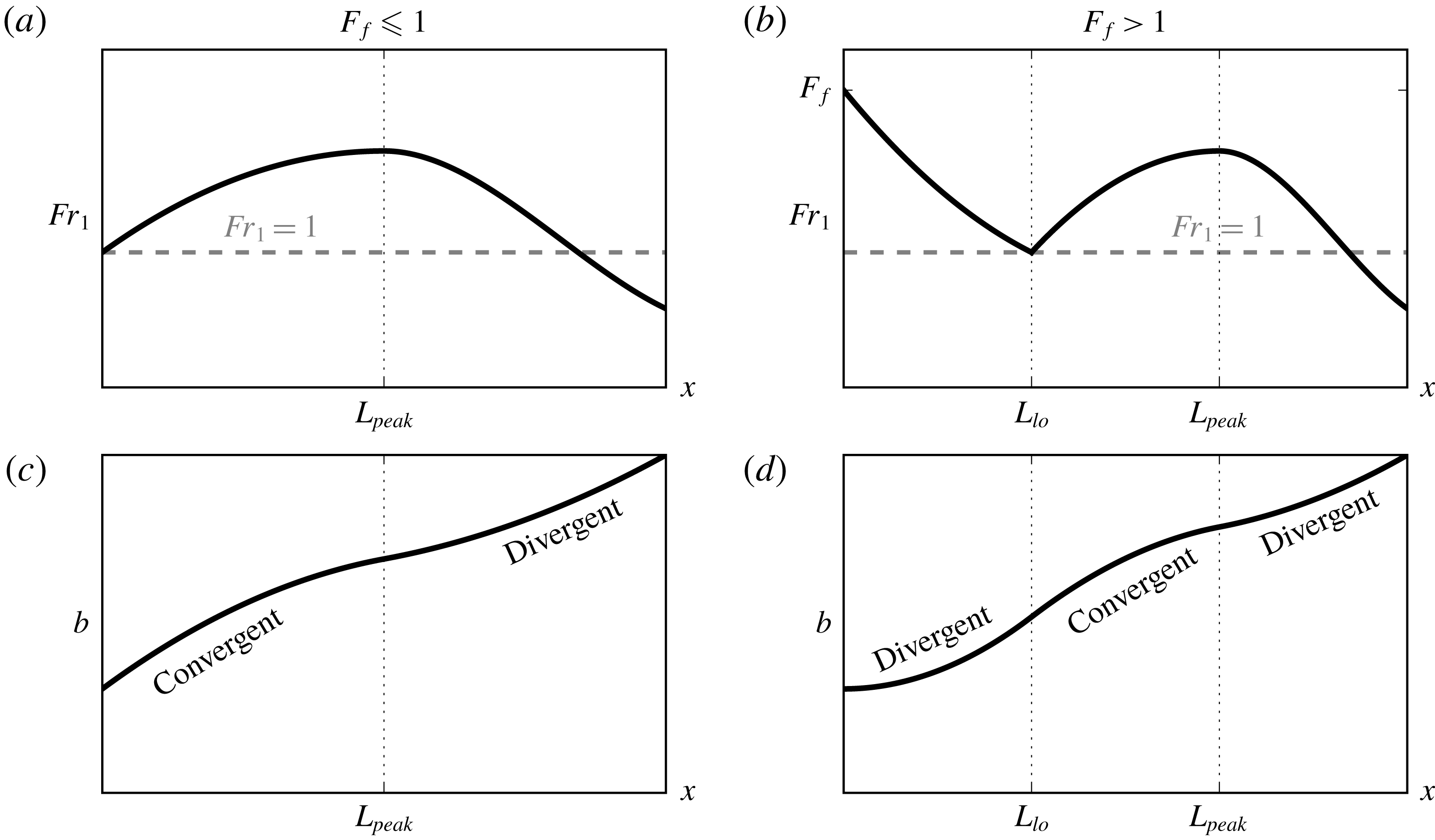
) cases. This picture comes entirely from the Froude number dynamics of a single active layer in the vicinity of a control point as described in Armi & Farmer (Reference Armi and Farmer1986), and it is described in further detail in § 2.3 below.
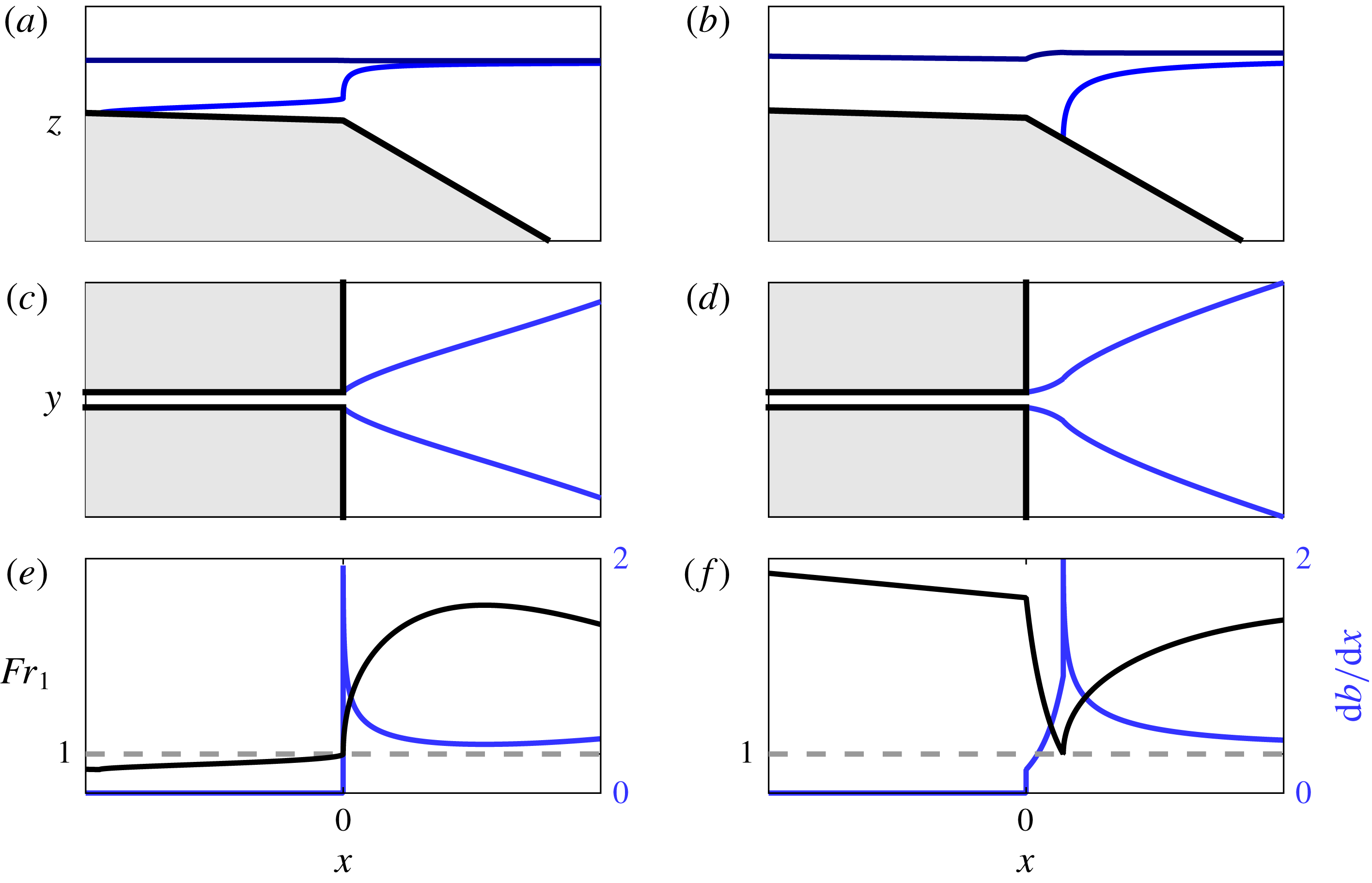
Schematic showing the anticipated evolution of upper layer Froude number
 $Fr_{1}$
(a,b) and plume width
 $b$
(c,d) in the offshore direction from the river mouth in the subcritical (
 $F_{f}\leqslant 1$
, a,c) and supercritical (
 $F_{f}>1$
, b,d) cases. The location of liftoff,
 $L_{lo}$
, and the location of the peak Froude number after liftoff,
 $L_{peak}$
, are indicated. The regions of convergent and divergent plume spreading are also indicated. Note that these predictions are a consequence of only two assumptions: (i) the plume behaves hydraulically, and (ii) plume spreading is driven by its buoyancy.

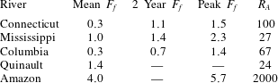
Aspect ratio and mean, two year flood and peak values of freshwater Froude number
 $F_{f}$
based on mean, two year flood and peak recorded river flow and river mouth geometry in natural systems. A dash (
 $-$
) indicates that the corresponding discharge value (two year recurring or maximum recorded) was not readily available.
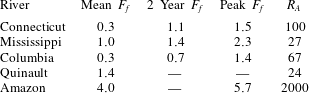
For reference, we show in table 1 estimates of the mean, two year recurring and peak freshwater Froude numbers calculated for several natural systems based on their mean, two year flood and peak recorded river discharges, along with estimated mean depths and widths at their mouths. The two year flood is particularly relevant morphodynamically, as it represents roughly the point of optimization between frequency of occurrence and sediment carrying capacity and is often used as a characteristic discharge in morphodynamic modelling (e.g. Chatanantavet et al.
Reference Chatanantavet, Lamb and Nittrouer2012). The peak discharge for the Connecticut river is estimated based on peak flood discharges recorded after Hurricane Irene (August 2011, Yellen et al.
Reference Yellen, Woodruff, Kratz, Mabee, Morrison and Martini2014). The peak discharge for the Mississippi corresponds to the 1927 flood, which is the largest flood on record (Lamb et al.
Reference Lamb, Nittrouer, Mohrig and Shaw2012). With the exception of the Amazon, which is exceptional both in the magnitude of its discharge and the wide and narrow cross-section of its mouth, typical values of
 $F_{f}$
range between
 $O(0.1)$
and
 ${\sim}1{-}3$
. Also shown in table 1 are the estimated inflow aspect ratios
 $R_{A}\equiv b_{0}/h_{0}$
, one of the dimensionless parameters that will be important in the subsequent analysis. We note that, again with the exception of the Amazon, typical field values of
 $R_{A}$
are
 $O(10{-}100)$
.
The values of
 $F_{f}$
indicated in table 1 are calculated taking into account the river discharge only. In fact, each of the systems listed are tidal, and the theory developed here can be applied in a quasi-steady sense to predict the structure of the salt wedge and peak intrusion length as the tide transitions from flood to ebb (Geyer & Farmer Reference Geyer and Farmer1989; Geyer & Ralston Reference Geyer, Ralston, Wolanski and McLusky2011; Poggioli & Horner-Devine Reference Poggioli and Horner-Devine2015) or the structure the quasi-steady near-field plume during mid-to-late ebb up to early flood (Hetland & MacDonald Reference Hetland and MacDonald2008). However, the effective discharge would then be the sum of the river discharge and a tidal component. The tidal flux can be as large or much larger than the river discharge, and it is routinely observed in strongly tidal salt wedge estuaries that the saline intrusion is fully washed out during ebb tide (e.g. Hughes & Rattray Reference Hughes and Rattray1980; Geyer & Farmer Reference Geyer and Farmer1989; Hetland & MacDonald Reference Hetland and MacDonald2008), indicating the occurrence of supercritical values of the effective freshwater Froude number.
Three remarks are appropriate before leaving this discussion. First, we note some confusion in the terminology. We refer to as subcritical (supercritical) both the regions of the flow where
 $Fr_{1}<1$
(
 $Fr_{1}>1$
) and the case that the freshwater Froude number
 $F_{f}<1$
(
 $F_{f}>1$
). The former describes the local hydraulic state of the upper layer, based on the upper layer Froude number, while the latter describes the overall regime of the system, predicting whether the liftoff point will be in the river channel or on the shelf. This terminology is standard and we will continue to use it here, taking care to be explicit when confusion may arise. Second, we also note that in the above discussion we have been concerned only with baroclinic criticality, pertaining to the interfacial long wave mode and relevant to the density-driven dynamics of two-layer flows. It is also possible for the flow to become barotropically supercritical, pertaining to the free-surface long wave mode. This occurs when
 $F_{e}\equiv Q/b_{0}\sqrt{gh_{0}^{3}}\equiv \sqrt{\unicode[STIX]{x0394}\unicode[STIX]{x1D70C}_{0}/\unicode[STIX]{x1D70C}_{2}}\,F_{f}>1$
. In this case, no hydraulic solution for the structure of the plume exists. For the large majority of natural systems, this would correspond to a discharge event that is too extreme to ever occur. As discussed below, our theoretical developments predict that some of our highest
 $F_{f}$
experimental runs should fall within this regime. We will not develop a theoretical description of this regime here, as it is not relevant to our understanding of natural estuarine–plume systems. Finally, we note that the fact that the control point is washed offshore at a critical value of unity in the freshwater Froude number, a quantity defined in terms of properties at the mouth, is a reflection of the assumption that the mouth acts as hydraulic control when the flow is subcritical, i.e. when
 $F_{f}<1$
. Thus, insofar as the experimental evidence presented below indicates a transition in behaviour of the plume at
 $F_{f}=1$
that is consistent with washing out of the control point at the river mouth and formation of an offshore liftoff front if and only if
 $F_{f}>1$
, it provides indirect evidence that the river mouth indeed acts as hydraulic control.
2.2 Buoyant spreading
We must also specify how we are to close our one-dimensional model of the buoyant layer seaward of the mouth, where the flow is no longer laterally confined and thus the plume width
 $b$
itself becomes a dependent variable. Bondar (Reference Bondar1970) first proposed that the lateral spreading of a buoyant surface-trapped plume is driven principally by the cross-flow baroclinic pressure gradient and may therefore be related to the local internal gravity wave speed
 $c=\sqrt{g^{\prime }h_{1}}$
. This assumption was implemented in a simple layer model of the Mississippi River plume by Wright & Coleman (Reference Wright and Coleman1971) and compared favourably to the plume width inferred from satellite-based observations of turbidity and sea surface temperature. In this study, the authors identify a near-field plume that is separated from the coast and is nearly uniform in the cross-flow direction. However, the well-confined, uniform structure of the Mississippi plume observed by Wright & Coleman (Reference Wright and Coleman1971) is likely due at least in part to the presence of ambient stratification and currents in the receiving basin, complications we do not consider here.
More recently, the buoyant spreading hypothesis has been tested favourably in field (Chen et al. Reference Chen, MacDonald and Hetland2009) and numerical (Hetland & MacDonald Reference Hetland and MacDonald2008) studies of the Merrimack river plume. In these studies, the authors identify a near-field core in the vicinity of the river mouth where plume properties are essentially constant in the cross-flow direction, and they find that this core spreads locally according to the internal gravity wave speed. These studies inspired laboratory experiments investigating the relationship between lateral spreading and vertical entrainment in the surface-trapped plume (Yuan & Horner-Devine Reference Yuan and Horner-Devine2013); while these authors did not directly investigate whether the internal gravity wave speed could be used to effectively parameterize the spreading rate, they did observe a transition from convergent to divergent spreading at a critical freshwater Froude number of approximately one. (See their figure 5.) As will be further discussed in § 2.3 below, this transition in the plume spreading behaviour is characteristic of the buoyant spreading and hydraulic behaviour of the plume.
The Merrimack studies also inspired theoretical work on a generic description of the quasi-steady near-field plume dynamics (Hetland Reference Hetland2010). In this study, a two-layer model identical to the one applied here for the surface-trapped plume was compared to an idealized numerical model of the quasi-steady near-field plume forming after passage of the plume front. The comparisons indicated that the two-layer model effectively described the evolution of the homogeneous core of the plume, including both the plume width and the dilution of the plume water in the along-flow direction. However, we note that the results had to be adjusted in order to account for the influence of the Coriolis force. This is consistent with the results of McCabe, MacCready & Hickey (Reference McCabe, MacCready and Hickey2009), who performed numerical simulations of the Columbia River plume and found that both the baroclinic cross-flow density gradient and the Coriolis force were important in determining the lateral spreading rate of the near-field plume. It is also consistent with the numerical and observational results of Chen et al. (Reference Chen, MacDonald and Hetland2009) for the Merrimack plume, who find that Coriolis and buoyancy (along with streamline curvature and interfacial stress) both contribute to the plume spreading within
 $3.5{-}7$
channel widths of the river mouth, while a balance between the Coriolis force and streamline curvature dominates further offshore. Indeed, neglect of rotational effects, along with ambient flow and stratification in the receiving basin, is a limitation of our highly idealized theoretical description, and there is undeniably a need for more systematic investigation of the factors influencing plume spreading across more natural systems. Nonetheless, in the aforementioned studies of plume spreading, buoyancy is universally found to contribute significantly to the plume spreading, and we will leave an investigation of additional complications induced by, e.g. rotation to future work.
Following Hetland & MacDonald (Reference Hetland and MacDonald2008), Chen et al. (Reference Chen, MacDonald and Hetland2009) and Hetland (Reference Hetland2010), we conceptualize the surface-trapped plume as spreading laterally like a finite-volume gravity current. In the case of a gravity current in a semi-infinite ambient basin, the frontal propagation speed of the current
 $u_{F}$
is given by
 $u_{F}/\sqrt{g^{\prime }h_{1}}=1$
(Shin, Dalziel & Linden Reference Shin, Dalziel and Linden2004). With this relation we find for a steady, one-dimensional flow
 $\text{D}b/\text{D}t=u\,\text{d}b/\text{d}x=2\sqrt{g^{\prime }h_{1}}$
, yielding, for the surface-trapped plume,
 $$\begin{eqnarray}\frac{\text{d}b}{\text{d}x}=\frac{2}{Fr_{1}}.\end{eqnarray}$$
The factor of two comes from the fact that the plume spreads on either side.
In extending our theory to the case that
 $F_{f}>1$
, we must also make an assumption about the parameterization of the spreading rate in the bottom-attached plume forming between the river mouth and liftoff front. This situation is complicated by (i) the bidirectional nature of lock-exchange flow, (ii) the influence of lateral entrainment-driven (i.e. jet-like) spreading when the momentum flux is large compared to the buoyancy flux, i.e. when
 $F_{f}\gg 1$
and possibly by (iii) the development of significant lateral barotropic pressure gradients when
 $F_{f}\gg 1$
– see figure 11 below. The latter two effects are anticipated to become significant only for very large freshwater Froude numbers, when the influence of the plume buoyancy becomes secondary to the momentum and the dynamics induces significant variations in free-surface elevation relative to sea level. We refer to this as the jet-like regime.
On the other hand, when the plume is supercritical (
 $F_{f}>1$
), but the freshwater Froude number is still of order one, we anticipate the the plume buoyancy will still significantly influence the plume spreading. On general scaling grounds, we anticipate that the buoyancy-driven spreading rate of the bottom-attached plume to behave as
 $\text{d}b/\text{d}x=\unicode[STIX]{x1D705}/Fr_{1}$
, as in the surface-trapped plume. In this relationship,
 $\unicode[STIX]{x1D705}$
is a coefficient of proportionality. We emphasize that what is relevant dynamically in the one-dimensional model developed below is the depth-averaged plume width,
 $b$
. We constrain the range of
 $\unicode[STIX]{x1D705}$
by considering the dynamics of lock-exchange gravity currents of the type treated extensively by Benjamin (Reference Benjamin1968). Benjamin (Reference Benjamin1968) shows that energy conservation in an inviscid, symmetric lock-exchange flow requires the formation of two counter-directed gravity currents, each occupying half the layer depth and propagating at a speed
 $u_{F}=\sqrt{g^{\prime }h}/2$
, where
 $h$
is the total fluid depth. In this case, the depth-averaged spreading rate would vanish, as the influx of dense fluid into the cross-section would exactly counter the efflux of lighter fluid out of the cross-section. On the other hand, if the lighter fluid were to occupy the entire depth, the total spreading rate would be
 $\text{d}b/\text{d}x=2\times (\sqrt{g^{\prime }h}/2)/u=1/Fr_{1}$
, corresponding to
 $\unicode[STIX]{x1D705}=1$
. This would, however, require a significant transfer of energy from the longitudinal to the transverse direction (Benjamin Reference Benjamin1968; Shin et al.
Reference Shin, Dalziel and Linden2004).
This picture is complicated by the influence of dissipation both at the interface between the intruding (dense) and outflowing (buoyant) gravity currents, as well as at the solid boundary in contact with the lower intruding gravity current. To our knowledge, there has been little work systematically investigating the influence of bottom friction on dense gravity currents produced by symmetric lock exchange. More generally, the structure of the bottom-attached plume, and the influence of transverse, buoyantly driven processes on the longitudinal, hydraulically controlled processes discussed here is an important topic in need of further attention. Here, we assume the dominance of buoyant spreading in the bottom-attached plume, assuming a spreading rate of the form
 $\text{d}b/\text{d}x=\unicode[STIX]{x1D705}/Fr_{1},\unicode[STIX]{x1D705}\in [0,1]$
, and we will explore the sensitivity of our model predictions to the parameter
 $\unicode[STIX]{x1D705}$
. Ultimately, we find that, at the field scale and for reasonable values of the shelf slope
 $\unicode[STIX]{x1D6FC}_{S}$
, the predictions for both liftoff length and superelevation at the river mouth are relatively insensitive to the particular value of
 $\unicode[STIX]{x1D705}$
used (figure 10
b,c). Based on the above considerations, we impose for the spreading rate
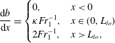 $$\begin{eqnarray}\frac{\text{d}b}{\text{d}x}=\left\{\begin{array}{@{}ll@{}}0,\quad & x<0\\ \unicode[STIX]{x1D705}Fr_{1}^{-1},\quad & x\in (0,L_{lo})\\ 2Fr_{1}^{-1},\quad & x>L_{lo},\end{array}\right.\end{eqnarray}$$
where
 $\unicode[STIX]{x1D705}\in [0,1]$
, as noted above, and
 $L_{lo}$
is the liftoff length – see figures 1 and 2.
Finally, we note that this description of spreading is distinct from the assumption of a symmetric, radially spreading plume that is typically incorporated in descriptions of the plume front dynamics (e.g. Garvine Reference Garvine1984; O’Donnell Reference O’Donnell1988; Jay, Zaron & Pan Reference Jay, Zaron and Pan2010; Kilcher & Nash Reference Kilcher and Nash2010). Indeed, we are not interested here in the unsteady dynamics of the plume front, but instead in the structure of the quasi-steady near-field plume forming soon after passage of the front (Hetland & MacDonald Reference Hetland and MacDonald2008; Hetland Reference Hetland2010). The front is relatively isolated from the influence of the river momentum, instead propagating radially under the influence of its own buoyancy as a gravity current (Garvine Reference Garvine1984; Luketina & Imberger Reference Luketina and Imberger1987; Kilcher & Nash Reference Kilcher and Nash2010). On the other hand, the quasi-steady near-field plume forming in the vicinity of the river mouth after the front has passed is strongly influenced by the river momentum, and the assumption of radial spreading is no longer strictly valid. In our theoretical description, we follow Hetland (Reference Hetland2010), who found that the offshore evolution of the near-field plume can be effectively described by considering flow only in the homogeneous core of the plume. While it is true that our simplified description of the plume spreading and the fact that we consider only a steady state plume means that we cannot capture processes associated with the plume front, our ability to reproduce the qualitative structure of the experimentally derived plume widths (figures 4 and 8) and the magnitude and trend of the liftoff length as a function of freshwater Froude number (figure 9) suggests that the simplified description presented here adequately characterizes the structure of the quasi-steady near-field plume.
2.3 Conceptual model
We develop a conceptual model of the offshore evolution of the plume by combining the hypothesis that the flow behaves hydraulically in both the subcritical and supercritical regimes with the buoyant spreading hypothesis. From Armi & Farmer (Reference Armi and Farmer1986), we anticipate qualitatively distinct along-flow profiles of
 $Fr_{1}$
in the subcritical (
 $F_{f}<1$
) and supercritical (
 $F_{f}>1$
) cases. When
 $F_{f}<1$
, the flow is subcritical in the river, and the river mouth acts as hydraulic control. This forces
 $Fr_{1}$
to increase in the downstream direction in the river so that
 $Fr_{1}=1$
at the river mouth, and it continues to increase offshore as the plume shoals, thins and accelerates (figure 1
a). The offshore increase of the upper layer Froude number is counteracted by interfacial friction and the entrainment of negative relative momentum from the ambient basin. This results in a peak value of
 $Fr_{1}$
occurring somewhere offshore of the mouth, at a location designated
 $x=L_{peak}$
. Beyond this point,
 $Fr_{1}$
continues to decrease, eventually passing continuously through
 $Fr_{1}=1$
and returning to the subcritical solution branch. This anticipated evolution of the upper layer Froude number is shown schematically in figure 1(a).
When
 $F_{f}>1$
, the upper layer Froude number is supercritical in the river, and the control point is washed out of the river mouth. Because the freshwater Froude number is defined in terms of the total depth at the river mouth, and there is no intrusion of salt water into the river when
 $F_{f}>1$
, we have
 $Fr_{1}=F_{f}$
at the river mouth. The buoyant layer will not immediately detach from the seabed, resulting in a laterally spreading bottom-attached plume. The increase in cross-sectional area causes the plume to decelerate and the upper layer Froude number to decrease until
 $Fr_{1}=1$
. We designate the location where this happens as
 $x=L_{lo}$
because the critical Froude number causes the buoyant layer to detach from the seabed and a liftoff front to form. Beyond this point, the evolution of
 $Fr_{1}$
is qualitatively the same as in the subcritical case described above. We show the evolution of
 $Fr_{1}$
in the supercritical regime schematically in figure 1(b).
We combine the anticipated evolution of
 $Fr_{1}$
described above with the buoyant spreading hypothesis, as encapsulated in (2.2). This equation implies that regions where
 $Fr_{1}$
increases are convergent, meaning
 $\text{d}^{2}b/\text{d}x^{2}<0$
, and regions where
 $Fr_{1}$
decreases are divergent,
 $\text{d}^{2}b/\text{d}x^{2}>0$
. From (2.2), we sketch the anticipated evolution of the plume width in figure 1, panels (c) (
 $F_{f}\leqslant 1$
) and (d) (
 $F_{f}>1$
). Importantly, this conceptual description requires that
 $L_{peak}$
correspond to a transition in curvature from convergent to divergent, and
 $L_{lo}$
to a transition from divergent to convergent. In what follows, we will concentrate on the latter curvature length scale, as it is anticipated to offer a robust bulk indication of the location of hydraulic transition and liftoff in the plume. Thus, the conceptual model predicts that
 $L_{peak}$
will increase monotonically with
 $F_{f}$
, moving offshore as
 $F_{f}$
is increased above one, and disappearing when
 $F_{f}\leqslant 1$
. We will formulate this model in the context of two-layer hydraulics in § 3, and we will test the predictions of this theory experimentally in § 4.
3 Theory
Our aim in this section is to develop a simplified theoretical description of the hydrodynamics that captures the structure of the flow. We want to solve for interfacial shape, plume width and liftoff location as a function of the freshwater Froude number, inflow aspect ratio, and river and shelf slopes. To this end, we adopt the framework of hydraulic theory, as discussed above. We will apply and extend previous work presented in Schijf & Schönfeld (Reference Schijf and Schönfeld1953), Hetland (Reference Hetland2010) and Poggioli & Horner-Devine (Reference Poggioli and Horner-Devine2015). In contrast to previous work, we do not limit our description to the case where conditions at the river mouth are known, allowing us to extend this theory to the case in which a liftoff front is formed offshore of the river mouth when
 $F_{f}>1$
. Additionally, we will experimentally test the predictions of the hydraulic theory presented in Poggioli & Horner-Devine (Reference Poggioli and Horner-Devine2015) for the shape and length of the salt wedge intrusion in a sloped channel, and (indirectly) the assumption that the plume spreads laterally as a gravity current commonly discussed in the literature (e.g. Wright & Coleman Reference Wright and Coleman1971; Hetland & MacDonald Reference Hetland and MacDonald2008; Chen et al.
Reference Chen, MacDonald and Hetland2009; Hetland Reference Hetland2010; Yuan & Horner-Devine Reference Yuan and Horner-Devine2013). Finally, we will develop analytical predictions for the free-surface elevation at the mouth as a function of the river discharge, which has implications for the hydraulic structure of the flow in the river and thus for the suspension of sediment and export to the shelf. This solution can be compared with the results of Lamb et al. (Reference Lamb, Nittrouer, Mohrig and Shaw2012), who present the hydraulic solution for a river entering the ocean as a function of imposed plume spreading angle but do not include the dynamics associated with the density contrast or buoyant plume processes.
Henceforth, unless explicitly stated otherwise, we use the following non-dimensioned independent and dependent variables:
 $x=\widetilde{x}/b_{0}$
,
 $b=\widetilde{b}/b_{0}$
,
 $\unicode[STIX]{x0394}\unicode[STIX]{x1D70C}=\unicode[STIX]{x0394}\widetilde{\unicode[STIX]{x1D70C}}/\unicode[STIX]{x0394}\unicode[STIX]{x1D70C}_{0}$
,
 $h_{1}=\widetilde{h}_{1}/h_{0}$
,
 $h_{2}=\widetilde{h}_{2}/h_{0}$
,
 $\unicode[STIX]{x1D702}=\widetilde{\unicode[STIX]{x1D702}}/h_{0}$
,
 $u=\widetilde{u}/\sqrt{g_{0}^{\prime }h_{0}}$
and
 $Fr_{1}\equiv \widetilde{u}/\sqrt{\widetilde{g}^{\prime }\widetilde{h}_{1}}=u/\sqrt{\unicode[STIX]{x0394}\unicode[STIX]{x1D70C}h_{1}}$
. Here, a tilde (
 $\widetilde{\text{ }}$
) indicates a dimensioned variable,
 $\widetilde{x}$
is the offshore distance,
 $\widetilde{b}$
is the flow width,
 $\unicode[STIX]{x0394}\widetilde{\unicode[STIX]{x1D70C}}$
is the density contrast between the buoyant layer and ambient ocean water,
 $\widetilde{h}_{1}$
and
 $\widetilde{h}_{2}$
are respectively the buoyant and lower layer thicknesses,
 $\widetilde{\unicode[STIX]{x1D702}}$
is the free-surface elevation,
 $\widetilde{u}$
is the offshore velocity of the buoyant layer,
 $\widetilde{g}^{\prime }\equiv (\unicode[STIX]{x0394}\widetilde{\unicode[STIX]{x1D70C}}/\unicode[STIX]{x1D70C}_{2})g$
is the reduced gravitational acceleration and
 $Fr_{1}$
is the buoyant upper layer Froude number. Additionally,
 $b_{0}$
is the channel width,
 $h_{0}$
is the total water depth at the river mouth,
 $\unicode[STIX]{x0394}\unicode[STIX]{x1D70C}_{0}$
is the total density difference between fresh and ocean water and
 $g_{0}^{\prime }=(\unicode[STIX]{x0394}\unicode[STIX]{x1D70C}_{0}/\unicode[STIX]{x1D70C}_{2})g$
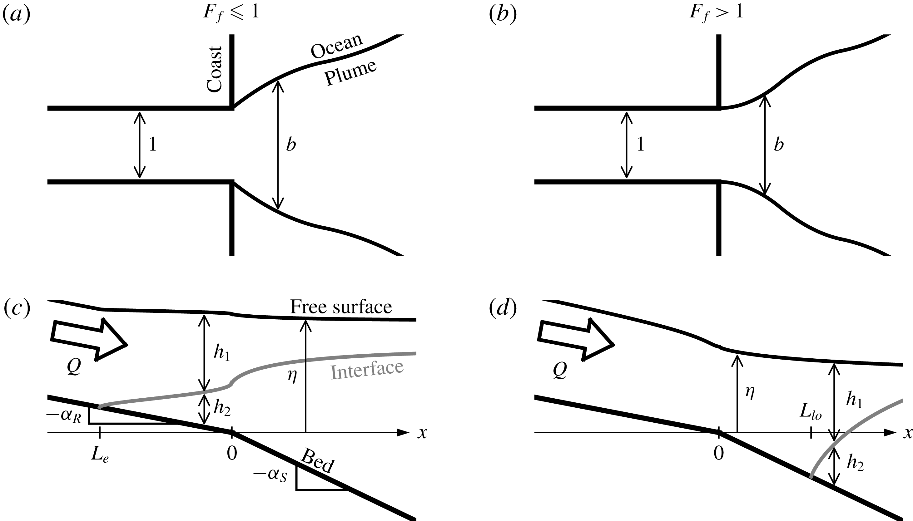
. See figure 2 for a depiction of the model domain and variables.
Schematic of the model domain and geometry in plan (a,b) and side (c,d) view for the subcritical (a,c) and supercritical (b,d) cases.
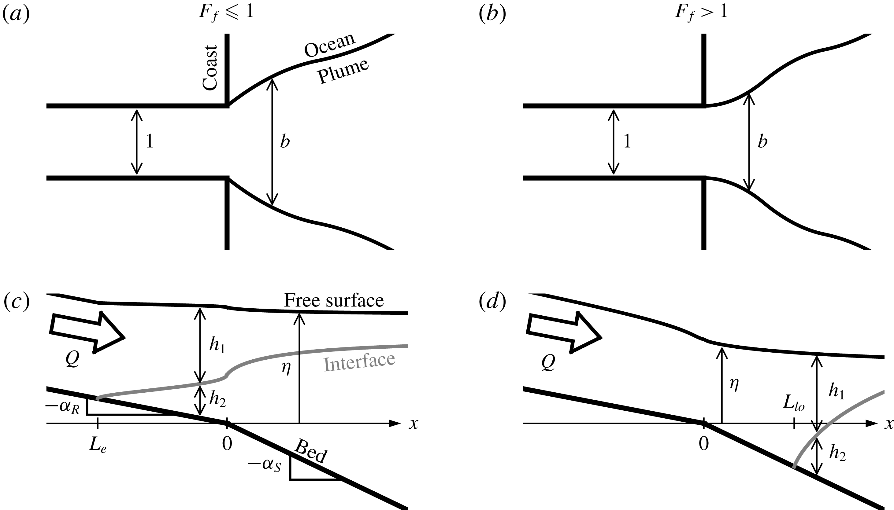
The flow in the plume and estuary is modelled as steady, one-dimensional, two-layer and hydrostatic. Each of the two layers are assumed to be of vertically uniform density and velocity, and the net flow in the lower layer is neglected. The dynamic influence of the width of the flow (set by the plume width or by the channel width in the case of the salt wedge intrusion) is included indirectly only through the continuity equation, and the plume width is parameterized on the assumption that the plume spreads laterally under the influence of its own buoyancy (2.2).
Frictional and mixing processes acting in the flow include interfacial and bottom shear stress, and lateral and vertical entrainment of mass and momentum. We parameterize the entrainment fluxes by introducing lateral and vertical entrainment velocities,
 $u_{L}$
and
 $u_{V}$
, respectively. We further introduce the lateral and vertical entrainment coefficients
 $\unicode[STIX]{x1D6FF}_{L}\equiv u_{L}/u$
and
 $\unicode[STIX]{x1D6FF}_{V}\equiv u_{V}/u$
, which are a priori functions of the local flow structure and turbulence properties (Ellison & Turner Reference Ellison and Turner1959; Christodoulou Reference Christodoulou1986; Princevac, Fernando & Whiteman Reference Princevac, Fernando and Whiteman2005). We parameterize the interfacial and bottom shear stress by introducing quadratic interfacial and bottom drag coefficients, respectively
 $C_{i}$
and
 $C_{D}$
, which we take to be constant throughout the model domain. In what follows, we develop the governing equations retaining all of these effects, and then afterwards look for the effects most relevant in the estuary, bottom-attached and surface-trapped plumes. In this way, we determine the simplest model that captures the structure of the flow, highlighting the most important physical mechanisms.
Finally, as discussed above, we will assume that the river mouth acts as a hydraulic control point when the freshwater Froude number is subcritical (
 $F_{f}<1$
), and that the liftoff front forms on the shelf when
 $Fr_{1}=1$
for supercritical freshwater Froude number (
 $F_{f}>1$
). Further, we will assume that far from the river mouth the water depth returns to a known value set by sea level (or by the imposed basin depth in our experiments).
3.1 Governing equations
Our model contains six independent flow variables:
 $Fr_{1}$
,
 $b$
,
 $\unicode[STIX]{x0394}\unicode[STIX]{x1D70C}$
,
 $h_{1}$
,
 $h_{2}$
and
 $\unicode[STIX]{x1D702}$
. Two equations come from conservation of water and salt mass, one from the imposed spreading rate and the final three come from the geometric and momentum conservation constraints particular to the one- or two-layer scenarios.
Integrating the conservation equations for salt and water mass at steady state, neglecting diffusive and turbulent diapycnal transport of mass in comparison to advective (entrainment) flux, and assuming a linear equation of state relating density to salt concentration, we find two simplified equations (Hetland Reference Hetland2010). The first imposes conservation of freshwater flux:
 $$\begin{eqnarray}Fr_{1}b(\unicode[STIX]{x0394}\unicode[STIX]{x1D70C}h_{1})^{3/2}=F_{f}.\end{eqnarray}$$
The second governs the dilution of plume water as it moves through the estuary and offshore:
 $$\begin{eqnarray}\frac{\text{d}\unicode[STIX]{x0394}\unicode[STIX]{x1D70C}}{\text{d}x}=-R_{A}\unicode[STIX]{x1D6FF}_{V}\frac{\unicode[STIX]{x0394}\unicode[STIX]{x1D70C}}{h_{1}}-2\unicode[STIX]{x1D6FF}_{L}\frac{\unicode[STIX]{x0394}\unicode[STIX]{x1D70C}}{b},\end{eqnarray}$$
where
 $R_{A}\equiv b_{0}/h_{0}$
is the inflow aspect ratio. In this equation, the first and second terms on the right-hand side govern, respectively, the vertical and lateral entrainment of mass into the buoyant layer. Only one or the other of these terms is relevant at a given location in the flow. Whereas lateral entrainment is the only means of dilution of a bottom-attached plume, when the plume is surface trapped, a partitioning of the entrainment flux into vertical and lateral components is not meaningful. In this case, all of the diapycnal entrainment flux is called vertical, and only this term is relevant.
As discussed in § 2.2 above, we parameterize the lateral spreading of the plume by assuming that it spreads laterally under the influence of its own buoyancy, and in particular that the surface-trapped plume spreads as a gravity current in an infinite ambient basin. The width is taken to evolve according to (2.2), and we will investigate the sensitivity of the plume structure to the parameter
 $\unicode[STIX]{x1D705}$
at the laboratory and field scale.
3.1.1 Two-layer flow
After liftoff, when there are two layers present, our geometric constraint becomes
 $$\begin{eqnarray}\unicode[STIX]{x1D702}=h_{1}+h_{2}-R_{A}\unicode[STIX]{x1D6FC}x,\end{eqnarray}$$
where
 $\unicode[STIX]{x1D6FC}$
is either the river or shelf slope, as appropriate. The upper and lower layer momentum equations give (see appendix A)
 $$\begin{eqnarray}\frac{\text{d}\unicode[STIX]{x0394}H}{\text{d}x}=-R_{A}\left[C_{i}\left(1+\frac{h_{1}}{h_{2}}\right)+\unicode[STIX]{x1D6FF}_{V}\right]\unicode[STIX]{x0394}\unicode[STIX]{x1D70C}Fr_{1}^{2},\end{eqnarray}$$
and
 $$\begin{eqnarray}\frac{\text{d}H_{2}}{\text{d}x}=R_{A}C_{i}\frac{h_{1}}{h_{2}}\unicode[STIX]{x0394}\unicode[STIX]{x1D70C}Fr_{1}^{2}.\end{eqnarray}$$
Here,
 $\unicode[STIX]{x0394}H\equiv H_{1}-H_{2}$
is the difference between the upper and lower layer hydraulic heads,
 $H_{1}$
and
 $H_{2}$
respectively. It is given by
 $$\begin{eqnarray}\unicode[STIX]{x0394}H\equiv \frac{1}{2}\left(\frac{F_{f}}{b\unicode[STIX]{x0394}\unicode[STIX]{x1D70C}h_{1}}\right)^{2}+\unicode[STIX]{x0394}\unicode[STIX]{x1D70C}h_{1}.\end{eqnarray}$$
The lower layer hydraulic head is given by
 $$\begin{eqnarray}H_{2}\equiv \left(\frac{\unicode[STIX]{x0394}\unicode[STIX]{x1D70C}_{0}}{\unicode[STIX]{x1D70C}_{2}}\right)^{-1}\unicode[STIX]{x1D702}-\unicode[STIX]{x0394}\unicode[STIX]{x1D70C}h_{1}.\end{eqnarray}$$
3.1.2 One-layer flow
Upstream of the liftoff point, there is no dense lower layer. Although only the freshwater layer is present, we retain the subscript
 $1$
on the flow variables for consistency with the two-layer equations developed above. In the case of a single layer, the geometry of the flow gives
 $$\begin{eqnarray}\unicode[STIX]{x1D702}=h_{1}-R_{A}\unicode[STIX]{x1D6FC}x.\end{eqnarray}$$
Further, as presented in appendix A, we find from the momentum equation
 $$\begin{eqnarray}\frac{\text{d}H}{\text{d}x}=R_{A}\unicode[STIX]{x1D6FC}-\frac{\unicode[STIX]{x0394}\unicode[STIX]{x1D70C}_{0}}{\unicode[STIX]{x1D70C}_{2}}\left(R_{A}C_{D}+2\unicode[STIX]{x1D6FF}_{L}\frac{h_{1}}{b}\right)\unicode[STIX]{x0394}\unicode[STIX]{x1D70C}Fr_{1}^{2},\end{eqnarray}$$
where
 $$\begin{eqnarray}H\equiv \frac{1}{2}\frac{\unicode[STIX]{x0394}\unicode[STIX]{x1D70C}_{0}}{\unicode[STIX]{x1D70C}_{2}}\left(\frac{F_{f}}{b\unicode[STIX]{x0394}\unicode[STIX]{x1D70C}h_{1}}\right)^{2}+h_{1}\end{eqnarray}$$
is the one-layer (open channel) hydraulic head (Chow Reference Chow1959). Note that
 $\unicode[STIX]{x0394}\unicode[STIX]{x1D70C}_{0}/\unicode[STIX]{x1D70C}_{2}$
appears here only as a consequence of our non-dimensionalization and the fact that we have written the hydraulic head in terms of
 $F_{f}$
instead of the barotropic Froude number
 $F_{e}\equiv \sqrt{\unicode[STIX]{x0394}\unicode[STIX]{x1D70C}_{0}/\unicode[STIX]{x1D70C}_{2}}F_{f}$
.
In (3.9), the term on the right-hand side proportional to
 $\unicode[STIX]{x1D6FF}_{L}$
and representing the lateral entrainment of momentum is relevant only in the case of a bottom-attached plume outside of the confines of the river.
Of course, in this case
 $h_{2}=0$
identically, as the flow has not detached from the bed. This provides our final constraint, closing our system of equations.
3.2 Boundary conditions
The flow variables are non-dimensionalized in terms of the properties at the river mouth. Thus,
 $$\begin{eqnarray}\unicode[STIX]{x0394}\unicode[STIX]{x1D70C}(0)=b(0)=h_{1}(0)+h_{2}(0)=\unicode[STIX]{x1D702}(0)=1.\end{eqnarray}$$
Further, from the condition that the flow is controlled at the mouth when
 $F_{f}<1$
we find
 $$\begin{eqnarray}h_{1}(0)=\left\{\begin{array}{@{}ll@{}}F_{f}^{2/3},\quad & F_{f}\leqslant 1\\ 1,\quad & F_{f}>1,\end{array}\right.\end{eqnarray}$$
and
 $$\begin{eqnarray}Fr_{1}(0)=\left\{\begin{array}{@{}ll@{}}1,\quad & F_{f}\leqslant 1\\ F_{f},\quad & F_{f}>1.\end{array}\right.\end{eqnarray}$$
In (3.12), the condition that
 $h_{1}(0)=F_{f}^{2/3}$
in the subcritical regime comes from imposing the critical depth at the mouth, that is the depth for which
 $Fr_{1}=1$
. In (3.13), the condition that
 $Fr_{1}(0)=F_{f}$
in the supercritical regime comes from the fact that the control is washed offshore of the mouth as
 $F_{f}$
increases above unity, and so the Froude number at the mouth is no longer critical but imposed by the value of
 $F_{f}$
.
3.3 Dimensionless parameters and solution methodology
The system of equations to be solved is given by (2.2), (3.1) and (3.2), and either (3.8) through (3.10) before liftoff, or (3.3) through (3.7) after liftoff. This system is subject to the boundary conditions given in (3.11) through (3.13). Together, these equations and boundary conditions indicate that the flow is governed by the following dimensionless parameters:
 $F_{f}$
,
 $\unicode[STIX]{x0394}\unicode[STIX]{x1D70C}_{0}/\unicode[STIX]{x1D70C}_{2}$
,
 $R_{A}$
,
 $\unicode[STIX]{x1D6FC}_{R}$
,
 $\unicode[STIX]{x1D6FC}_{S}$
,
 $C_{D}$
and
 $C_{i}$
. Additionally, the flow is affected by the imposed functional dependence of the entrainment coefficients on the local flow structure. For simplicity, and given the uncertainty in their variation at both the laboratory (Yuan & Horner-Devine Reference Yuan and Horner-Devine2013) and field (Princevac et al.
Reference Princevac, Fernando and Whiteman2005) scales, we will take
 $\unicode[STIX]{x1D6FF}_{L}$
and
 $\unicode[STIX]{x1D6FF}_{V}$
constant in what follows. Poggioli & Horner-Devine (Reference Poggioli and Horner-Devine2015) find that the normalized stratification
 $\unicode[STIX]{x0394}\unicode[STIX]{x1D70C}_{0}/\unicode[STIX]{x1D70C}_{2}$
has only a minor influence on the flow structure over the range of variation typical to the field (roughly
 $0.01$
–
 $0.02$
). Thus, given that all of our experiments were conducted at
 $\unicode[STIX]{x0394}\unicode[STIX]{x1D70C}_{0}/\unicode[STIX]{x1D70C}_{2}\approx 0.01$
, we will impose this as a fixed characteristic value in all of our calculations.
Additionally, we will find below that the influence of frictional and mixing processes on the qualitative flow structure is secondary, and it will typically be sufficient for our purposes to assume that the flow is inviscid and immiscible. This is not true in the estuary, where interfacial friction is the only means of arresting a saline intrusion in a channel of uniform width (Schijf & Schönfeld Reference Schijf and Schönfeld1953; Poggioli & Horner-Devine Reference Poggioli and Horner-Devine2015), and field observations indicate that frictional processes are a significant component of the salt wedge momentum balance and must be retained to obtain the correct structure for the pycnocline (Geyer et al. Reference Geyer, Ralston and Holleman2017).
Finally, we note that (2.2) is irrelevant for a salt wedge in a uniform channel. Further, if entrainment is negligible in the salt wedge, we may drop (3.2) and the second term on the right-hand side of (3.4) proportional to
 $R_{A}\unicode[STIX]{x1D6FF}_{V}$
. In this case we can introduce a rescaled along-flow coordinate
 $x_{\ast }\equiv R_{A}C_{i}x\equiv C_{i}\widetilde{x}/h_{0}$
. With this modification, the non-dimensional parameter space relevant to the immiscible salt wedge is reduced to
 $F_{f}$
,
 $C_{i}/\unicode[STIX]{x1D6FC}_{R}$
, and
 $\unicode[STIX]{x0394}\unicode[STIX]{x1D70C}_{0}/\unicode[STIX]{x1D70C}_{2}$
, provided that we also rescale the estuarine intrusion length as
 $L_{e}^{\ast }\equiv R_{A}C_{i}L_{e}\equiv C_{i}\widetilde{L}_{e}/h_{0}$
.
For a given set of non-dimensionalized parameters, numerical integration begins at the river mouth, where we impose the boundary conditions given in (3.11) through (3.13). In the subcritical case, integration of the two-layer equations continues upstream in the river channel until the interface intersects the channel bed, at which point the one-layer equations may be integrated an arbitrary distance further upstream. Likewise, the two-layer equations are integrated an arbitrary distance offshore to determine the structure of the supercritical plume. In solving the two-layer equations, we integrate to determine the evolution of
 $\unicode[STIX]{x0394}H$
and
 $H_{2}$
, and then use the cubic relationship between
 $h_{1}$
and
 $\unicode[STIX]{x0394}H$
given in (3.6) to solve for the upper layer depth. As is well known from the theory of hydraulic flow (e.g. Chow Reference Chow1959; Armi Reference Armi1986), this cubic relation contains two real solution branches, corresponding to the subcritical and supercritical regimes. It is necessary to choose the subcritical solution upstream of the control point and the supercritical solution downstream of the control point (see, e.g. Armi Reference Armi1986; Poggioli & Horner-Devine Reference Poggioli and Horner-Devine2015). A small revision to this point: in the case of the supercritical plume, friction and mixing allows the plume to relax gradually in the offshore direction through the critical point. In this case, the solution passes continuously (i.e. without passing through a hydraulic jump) from the supercritical back to the subcritical branch. This is observed in model runs when frictional and/or mixing processes in the plume are included, but we will not concentrate on this dynamics here, as we are interested primarily in the behaviour of the liftoff location.
In the supercritical case, the one-layer equations may be integrated an arbitrary distance upstream to determine the hydraulic structure of the flow in the river, and they are integrated offshore until
 $Fr_{1}=1$
. When the Froude number becomes critical, the upper layer detaches from the seabed and the liftoff front forms. After this point the two-layer equations are integrated to determine the structure of the supercritical surface-trapped plume. In the case of the experiments presented below, we were not readily able to measure the true dynamically adjusted water depth at the river mouth. What was accessible to us was instead the imposed elevation of the free surface in the basin far from the mouth, which coincides with the depth at the mouth of the channel prior to starting the experiment. We designate this elevation
 $h_{S}$
(sea level). In everything that follows, we will report the freshwater Froude number and aspect ratio calculated in terms of
 $h_{S}$
. Designating the values calculated in terms of the depth at the mouth by a superscript zero, we have
 $F_{f}=F_{f}^{0}/h_{S}^{3/2}$
and
 $R_{A}=R_{A}^{0}/h_{S}$
. Our model calculations indicate that the superelevation at the river mouth is a negligible fraction of
 $h_{S}$
when
 $F_{f}=1$
, indicating that the critical value of this redefined freshwater Froude number is still approximately one.
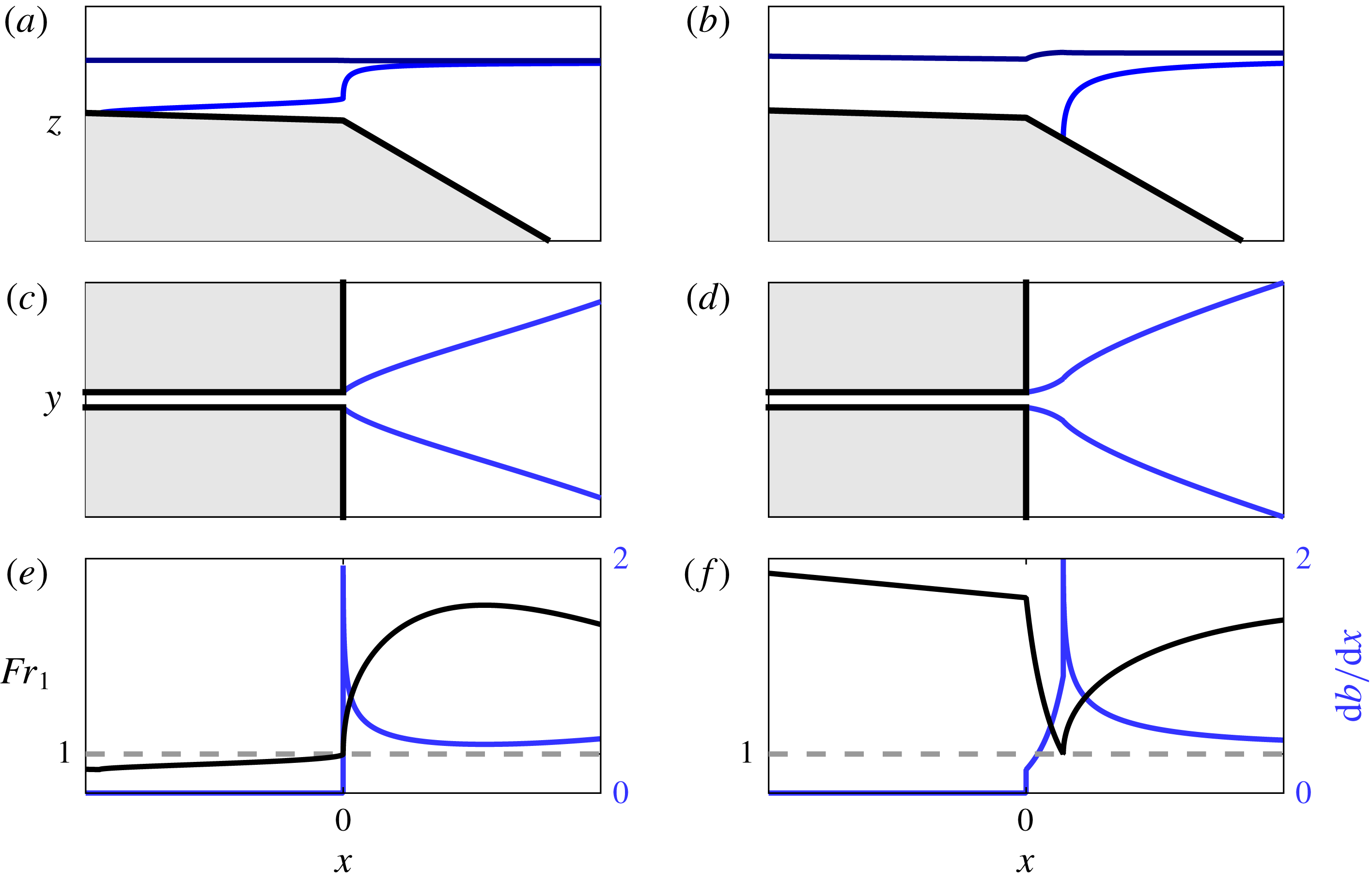
Model output for subcritical (
 $F_{f}=0.5$
, a,c,e) and supercritical (
 $F_{f}=5$
, b,d,f) cases. (a,b) Show the flow in side view, including the bed (thick black), interface (blue) and free surface (dark blue). (c,d) Show the flow in plan view, including the flow boundaries (thick black) and the lateral plume boundaries (blue). (e,f) Show the offshore evolution of the Froude number and flow width gradient
 $\text{d}b/\text{d}x$
. The dashed grey lines indicate
 $Fr_{1}=1$
. In panels (a)–(d), the grey shaded regions indicate solid boundaries outside of the flow domain. For both runs,
 $\unicode[STIX]{x0394}\unicode[STIX]{x1D70C}_{0}/\unicode[STIX]{x1D70C}_{2}=0.01$
,
 $R_{A}=10$
,
 $\unicode[STIX]{x1D6FC}_{R}=5\times 10^{-4}$
,
 $\unicode[STIX]{x1D6FC}_{S}=5\times 10^{-2}$
,
 $C_{i}=1\times 10^{-4}$
,
 $C_{D}=1\times 10^{-3}$
,
 $\unicode[STIX]{x1D705}=1$
and
 $\unicode[STIX]{x1D6FF}_{V}=\unicode[STIX]{x1D6FF}_{L}=0$
.
3.4 Analytical model results
Figure 3 shows sample model output for subcritical (
 $F_{f}=0.5$
, a,c,e) and supercritical (
 $F_{f}=5$
, b,d,f) runs. The remaining input parameters are as follows:
 $\unicode[STIX]{x0394}\unicode[STIX]{x1D70C}_{0}/\unicode[STIX]{x1D70C}_{2}=0.01$
,
 $R_{A}=10$
,
 $\unicode[STIX]{x1D6FC}_{R}=5\times 10^{-4}$
,
 $\unicode[STIX]{x1D6FC}_{S}=5\times 10^{-2}$
,
 $C_{i}=1\times 10^{-4}$
,
 $C_{D}=1\times 10^{-3}$
,
 $\unicode[STIX]{x1D705}=1$
and
 $\unicode[STIX]{x1D6FF}_{V}=\unicode[STIX]{x1D6FF}_{L}=0$
. As documented by the interface profiles (figure 3
a,b), a salt wedge forms for the subcritical run and a liftoff front forms that is pushed offshore of the river mouth for the supercritical run. We note that, whereas the deviation of the free surface height at the river mouth from sea level is negligible in the subcritical run, there is a pronounced decrease in the water depth at the mouth from sea level in the supercritical run, corresponding to a negative superelevation. As discussed above, the variation of the superelevation at the river mouth with discharge modifies the hydraulic structure of the flow in the river and has potentially significant impacts on the sediment transport in the river and export of sediment to the shelf (Lane Reference Lane1957; Chatanantavet et al.
Reference Chatanantavet, Lamb and Nittrouer2012; Lamb et al.
Reference Lamb, Nittrouer, Mohrig and Shaw2012). This is particularly important in the high discharge (supercritical) regime, which is anticipated to be most important for the evolution of the river morphology (Lamb et al.
Reference Lamb, Nittrouer, Mohrig and Shaw2012). We will explore the predictions of the model for the dependence of the superelevation as a function of freshwater Froude number and inflow aspect ratio in § 5 below.
The offshore evolution of the plume width (figure 3
c,d) and upper layer Froude number (figure 3
e,f) conform to our preliminary predictions for the relationship between the curvature of the plume spreading profile and the offshore evolution of the Froude number as shown schematically in figure 1. In particular, although subtle, in the subcritical width profile (figure 3
c) there is indeed a shift from convergent spreading as the Froude number initially increases offshore (figure 3
e) to divergent spreading as it peaks and then begins to decrease. The presence of this transition is confirmed in the profile of
 $\text{d}b/\text{d}x$
(figure 3
e). Likewise, in the supercritical width profile (figure 3
d) we clearly see an initially divergent region corresponding to the initial decrease of the Froude number in the bottom-attached plume before liftoff (figure 3
f), and a subsequent convergent region as the Froude number begins to increase again after liftoff. The location of the liftoff front is marked by a large cusp in the profile of
 $\text{d}b/\text{d}x$
(figure 3
f). The origin of this cusp is in the increase in spreading rate for a given upper layer Froude number as the plume detaches (2.2) and the discontinuity in the gradient of
 $Fr_{1}$
at liftoff. The magnitude of this cusp is dependent on the value of
 $\unicode[STIX]{x1D705}$
imposed in the model (
 $\unicode[STIX]{x1D705}=1$
here); however, for values of
 $\unicode[STIX]{x1D705}<1$
, the cusp in the spreading rate would be even more pronounced, and a transition in the spreading behaviour would be apparent even if the dominant spreading mechanism in the bottom-attached plume were other than buoyant spreading (e.g. linear, entrainment-driven spreading characteristic of a turbulent planar jet). For these reasons, this curvature transition is anticipated to be a robust indication of liftoff. In both cases, the model predicts that the Froude number in the surface-trapped plume will peak and then decrease, eventually falling below unity, only if friction and/or entrainment is included. Although the inclusion of friction and entrainment is important to capture correctly this long-distance behaviour, we will find below that the results of the inviscid, immiscible model will be enough to accurately characterize the qualitative features of our experimental results, including the evolution of the liftoff length with freshwater Froude number.
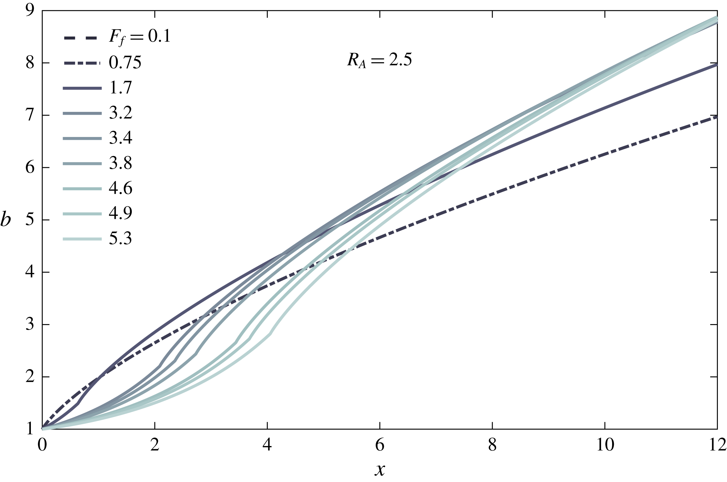
Model plume width profiles as a function of the freshwater Froude number at an inflow aspect ratio
 $R_{A}=2.5$
. Note that the freshwater Froude number and inflow aspect ratio are calculated in terms of sea level to correspond with the experiments – see main text. The parameters of the supercritical runs match the experimental runs shown in figure 8(a). The subcritical runs do not correspond to experimental runs but are included for comparison and completeness. The two subcritical runs precisely overlap in the figure. For all runs,
 $\unicode[STIX]{x1D6FC}_{R}=1.1\times 10^{-3}$
and
 $\unicode[STIX]{x1D6FC}_{S}=5\times 10^{-2}$
, corresponding to the experimental conditions of the supercritical runs. Additionally,
 $\unicode[STIX]{x1D705}=1$
, and
 $C_{i}=C_{D}=\unicode[STIX]{x1D6FF}_{V}=\unicode[STIX]{x1D6FF}_{L}=0$
.

We show in figure 4 predictions of the inviscid, immiscible two-layer equations for the offshore evolution of the plume width as a function of freshwater Froude number. The model parameters are selected to conform to our experiments (see figure 8). They are
 $R_{A}=2.5$
,
 $\unicode[STIX]{x1D6FC}_{R}=1.1\times 10^{-3}$
and
 $\unicode[STIX]{x1D6FC}_{S}=5\times 10^{-2}$
. Additionally, the supercritical runs correspond to experimentally realized values of the far-field freshwater Froude number
 $F_{f}$
. We observe two important features of the supercritical runs: first, they are initially sorted according to
 $F_{f}$
, with a higher value of
 $F_{f}$
corresponding to a narrower plume. However, as the plume evolves offshore, this sorting is not preserved. Second, in each of the supercritical runs there is an obvious length scale associated with the transition from divergent to convergent spreading behaviour and coinciding with the location of the liftoff front. As expected, this curvature scale is pushed offshore as
 $F_{f}$
is increased. We emphasize that the appearance of this curvature scale, and its offshore migration with increasing
 $F_{f}$
, is a consequence of both of our principal hypotheses: (i) that the dynamics of the plume may be described hydraulically, resulting in a predictable and consistent along-flow evolution of the Froude number, and (ii) that the spreading of the plume is driven principally by the buoyancy of the plume, resulting in a spreading rate
 $\text{d}b/\text{d}x\propto Fr_{1}^{-1}$
.
For the sake of comparison, we also include two subcritical profiles in figure 4, calculated for
 $F_{f}=0.1$
and
 $F_{f}=0.75$
. These do not correspond to experimentally realized runs. In the case of the inviscid, immiscible plume, for a given inflow aspect ratio, the subcritical profiles all collapse to the same curve. This conclusion is only slightly modified if we include for example the influence of interfacial friction acting on the plume, in which case we find that the deviation between runs with different values of
 $F_{f}$
is very slight, growing slowly in the offshore direction. Thus, we predict based on these results that, when normalized by channel width, the offshore evolution of the plume width should be nearly independent of the freshwater Froude number when
 $F_{f}<1$
. To our knowledge, this feature of subcritical plumes has not been noted before in the literature.
4 Experiments
4.1 Experimental apparatus and flow imaging
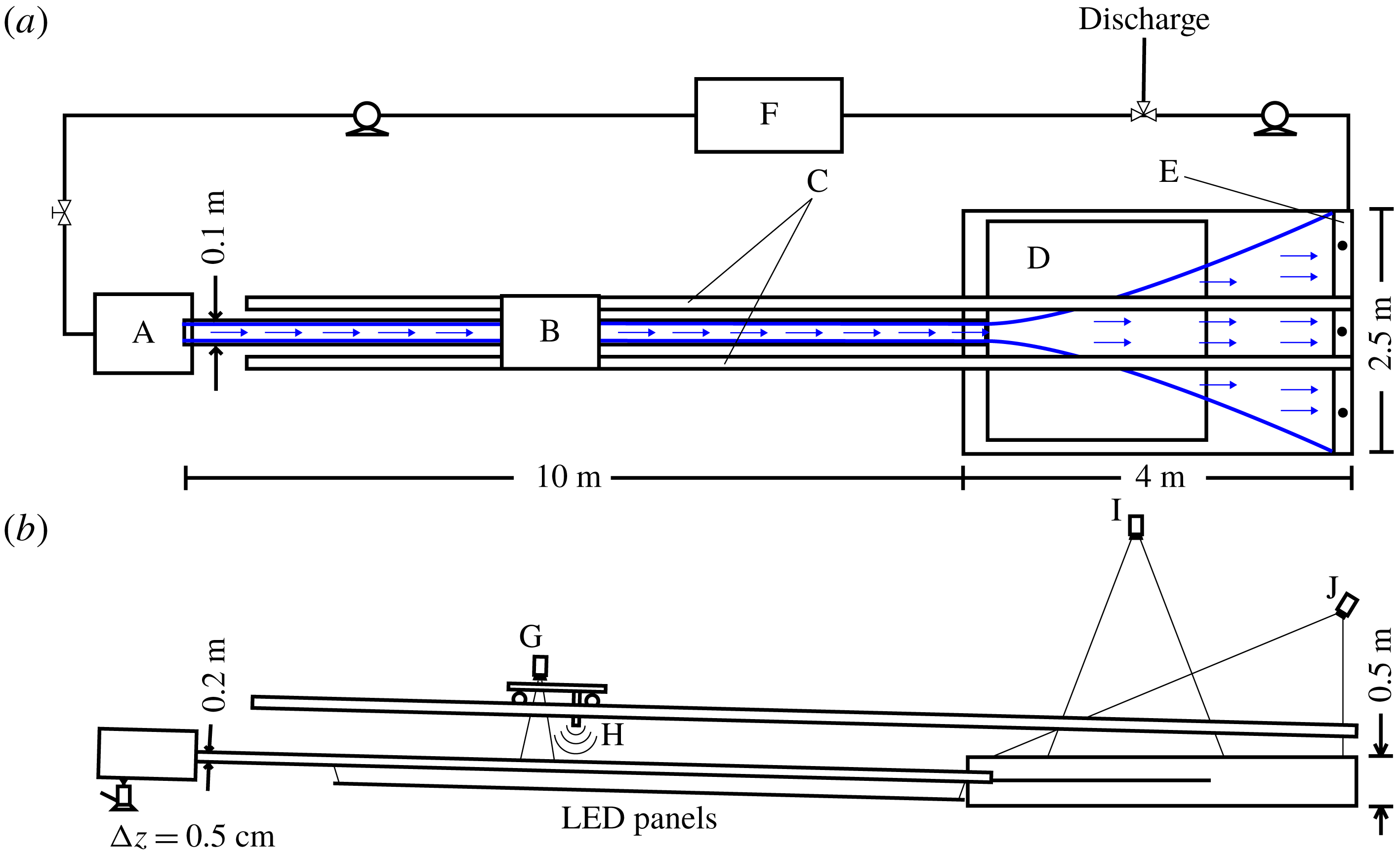
We have performed a set of experiments examining the interfacial structure of the salt wedge and the offshore evolution of the plume width. We show a schematic of the experimental apparatus in figure 5. During the experiments, freshwater is pumped from a large reservoir into a filling basin. The flowrate is controlled by a valve and flow meter on the line feeding into the filling basin. Water passes from the filling basin into an acrylic channel,
 $10~\text{m}$
long by
 $0.1~\text{m}$
wide by
 $0.2~\text{m}$
deep. This channel acts as our river and is supported by a series of vertically adjustable rigid connections to a steel panel spanning two steel channel sections, providing the rigidity necessary to allow us to precisely control the river slope. We can adjust the upstream channel elevation in
 $0.5~\text{cm}$
vertical increments, which corresponds to increments of the river slope of approximately
 $5.7\times 10^{-4}$
.
Schematic showing the experimental configuration in plan (a) and side (b) view. Key: (A) filling basin, (B) measurement cart, (C) aluminium tracks, (D) reflective shelf, (E) overflow weir, (F) freshwater source tank, (G) camcorder, (H) sonic altimeter, (I) overhead camera, (J) external light source.
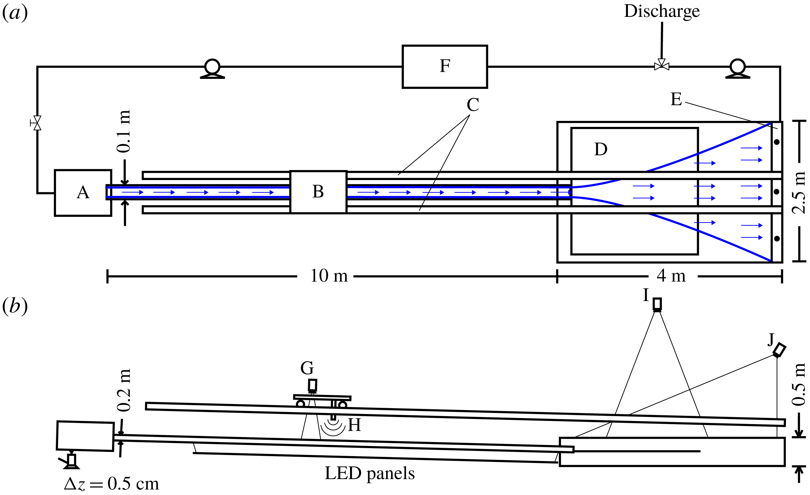
From this channel, the freshwater flows into an acrylic receiving basin,
 $4~\text{m}$
long by
 $2.5~\text{m}$
wide by
 $0.5~\text{m}$
deep (figure 5
a,b). We place a reflective panel in the receiving basin so that it meets the level of the channel at its mouth. This panel is maintained at a roughly uniform slope of
 $\unicode[STIX]{x1D6FC}_{S}=5\times 10^{-2}$
for all of the experiments and serves the dual purpose of coastal shelf and reflective surface for light from the external overhead light source, used when imaging the plume (figure 5
b). The imaging itself is performed using a camera suspended over the plume basin. We adjust the density in the basin by adding salt (NaCl) until the desired value of
 $\unicode[STIX]{x0394}\unicode[STIX]{x1D70C}_{0}/\unicode[STIX]{x1D70C}_{2}$
is obtained. The depth in the basin is adjusted to the desired level for the given experiment, and this level is maintained by an overflow weir that is positioned at the proper height (figure 5
a). The freshwater forms a buoyant surface-trapped layer in the plume (with the possible exception of an initial bottom-attached region in the supercritical runs) and flows across the length of the basin and over the weir, where it is then pumped to our discharge reservoir. There is a slow buildup of freshwater in the receiving basin owing to the two-layer flow structure over the overflow weir and to the fact that the plume width often exceeds the basin width at the downstream end of the basin. This backup is slow enough that a quasi-steady flow regime is readily obtained, but it does limit the maximum duration of the experiment.
When imaging the salt wedge, a motorized cart with a digital camcorder is run over aluminium tracks spanning the length of the river channel and the receiving basin (figure 5 a,b). In this case, uniform intensity LED panels placed under the channel are used to illuminate the flow. The motorized cart was also equipped with a sonic altimeter with the goal of obtaining profiles of the free surface elevation along the river and plume. However, it was found that these data were too noisy to resolve a meaningful signal, and they are not presented here.
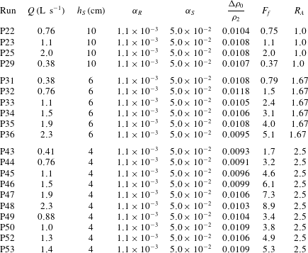
The experimental parameters corresponding to all of the runs presented in this manuscript are given in appendix B, tables 2 (salt wedge runs) and 3 (plume runs). In the experiments, we are able to adjust
 $F_{f}$
,
 $\unicode[STIX]{x0394}\unicode[STIX]{x1D70C}_{0}/\unicode[STIX]{x1D70C}_{2}$
,
 $R_{A}$
,
 $\unicode[STIX]{x1D6FC}_{R}$
and
 $\unicode[STIX]{x1D6FC}_{S}$
. Of these,
 $\unicode[STIX]{x0394}\unicode[STIX]{x1D70C}_{0}/\unicode[STIX]{x1D70C}_{2}$
and
 $\unicode[STIX]{x1D6FC}_{S}$
are held fixed for all experiments, at
 ${\sim}0.01$
and
 $5\times 10^{-2}$
, respectively. For all of the experiments the channel/inflow width is
 $b_{0}=10~\text{cm}$
.
In the experimental results presented below, we examine the interface between fresh and salt water in the salt wedge (figure 7), and the width of the plume (figure 8). Both are obtained using the optical thickness method (OTM) (Cenedese & Dalziel Reference Cenedese and Dalziel1998; Yuan, Avener & Horner-Devine Reference Yuan, Avener and Horner-Devine2011; Yuan & Horner-Devine Reference Yuan and Horner-Devine2013). In this method, one of the two water masses (fresh or salty) is dyed, and the intensity of attenuated light passing through the water column is related to the equivalent thickness
 $h_{eq}$
of the layer according to the Lambert–Beer law:
 $-\text{log}(I/I_{0})\propto h_{eq}$
. In this relation,
 $I$
is the intensity of attenuated light passing through the flow during the experiment, and
 $I_{0}$
is the intensity of light passing through an undyed layer under the same conditions. The background intensity is determined by recording images of undyed water in the experimental setup under experimental conditions before each run, and the constant of proportionality in the Lambert–Beer law depends on the dye concentration and is determined using cuvette calibration before each experiment. The equivalent layer thickness is equal to the true layer thickness in the limit that there is no mixing between the water masses.
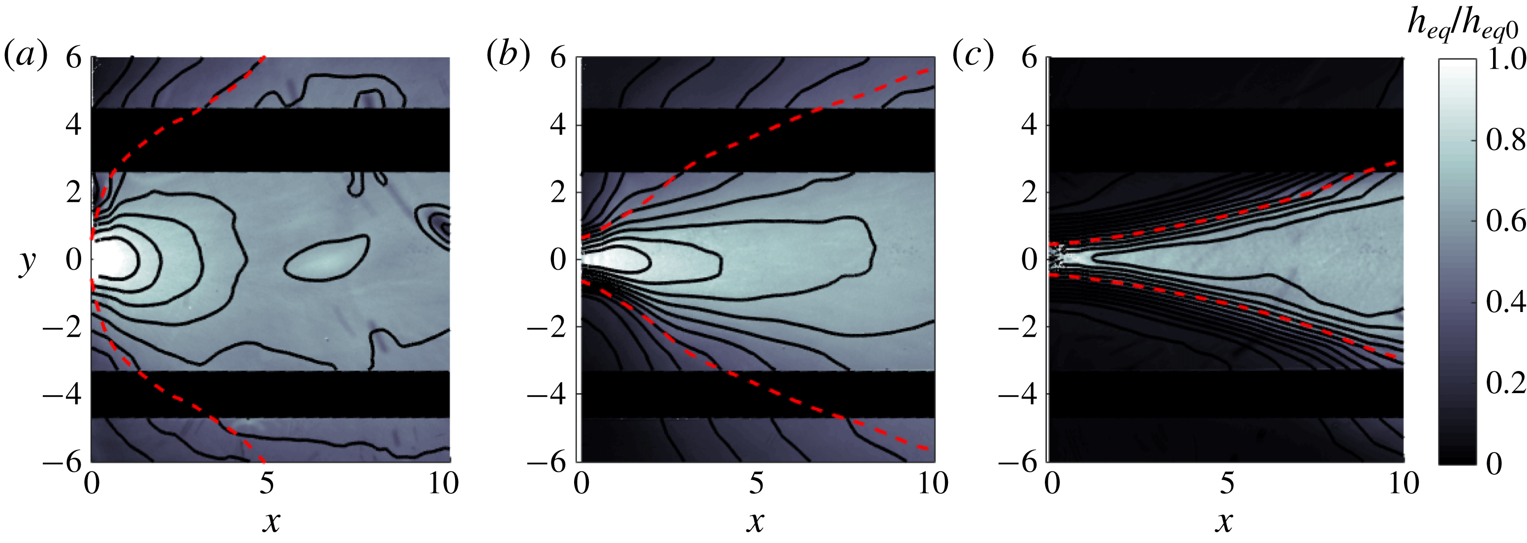
Plan view of two-dimensional equivalent plume thickness
 $h_{eq}$
fields obtained using OTM for a subcritical (a,
 $F_{f}=0.37$
,
 $R_{A}=1.0$
) and two supercritical (b,
 $F_{f}=3.4$
,
 $R_{A}=2.5$
and c,
 $F_{f}=8.9$
,
 $R_{A}=2.5$
) runs. The equivalent layer thickness is normalized by the value measured at the mouth of the channel (located at the centre left of each image). Smoothed contours of the equivalent layer thickness (solid black curves) and the plume width obtained by extracting the standard deviation of a Gaussian fit to the lateral profiles of
 $h_{eq}$
(dashed red curve) are also shown. The dark regions running across the length of the plume in each panel correspond to the regions blocked by the aluminium tracks supporting the instrument cart (figure 5).
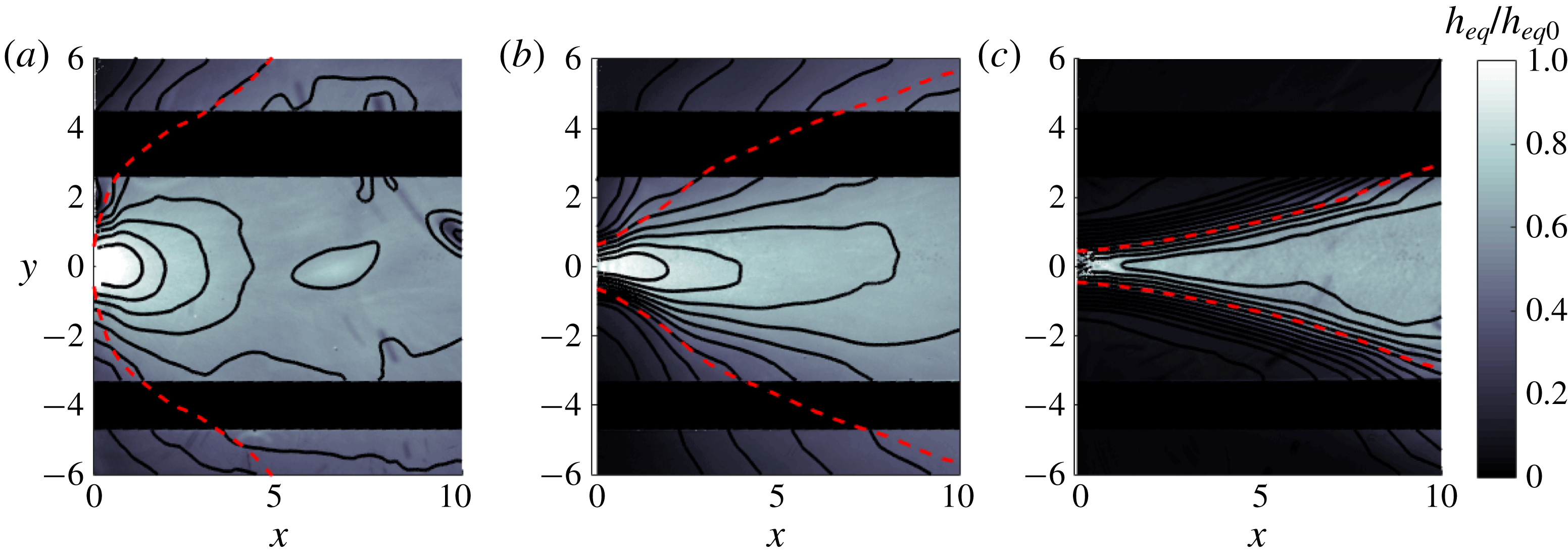
(a) Experimentally obtained profiles of salt wedge thickness for several values of
 $F_{f}$
and a fixed river slope
 $\unicode[STIX]{x1D6FC}_{R}=1.1\times 10^{-3}$
. The
 $x$
-coordinate is normalized by the measured intrusion length, and the salt wedge thickness is normalized by the theoretical value at the mouth,
 $h_{2}(0)=1-F_{f}^{2/3}$
. Also shown is a theoretical profile (red dashed line) obtained for the given river slope,
 $F_{f}=0.41$
, and a value of
 $C_{i}$
obtained from the fit to
 $Re$
discussed in the text and shown in the inset in the lower panel. (b) Intrusion length times aspect ratio (
 $L_{e}^{\ast }/C_{i}=R_{A}L_{e}$
) versus
 $F_{f}$
for four different values of the river slope. The theoretical curves are obtained using the fitted
 $C_{i}(Re)$
dependence shown in the inset.
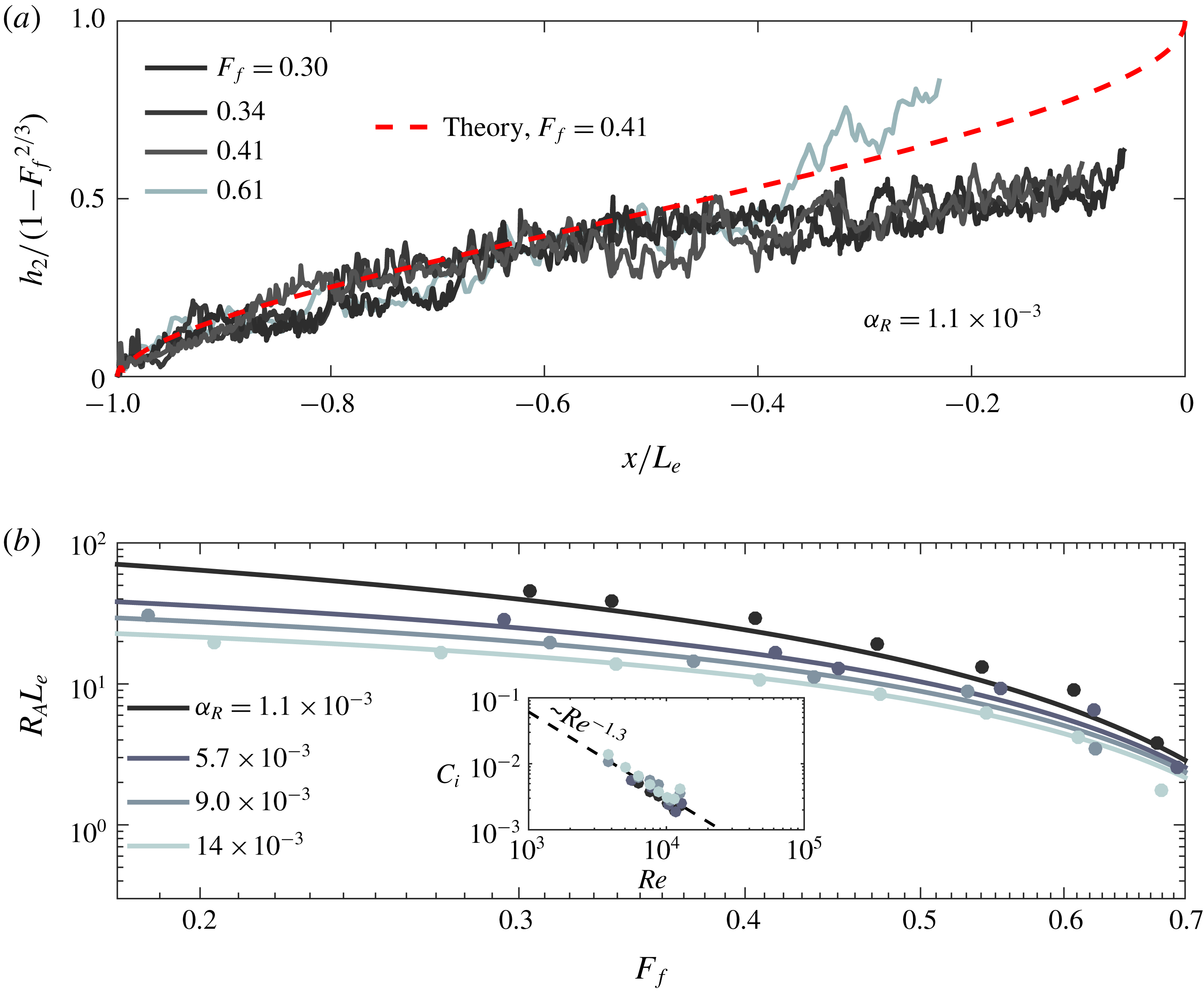
Which water mass is dyed is determined by whether we wish to image the salt wedge or the plume. For salt wedge runs, we dye the salt water layer, and we take images along the length of the channel using the camcorder mounted to the motorized cart (figure 5). The above analysis allows us to obtain the equivalent thickness of the salt wedge and thus the approximate vertical location of the interface. For the plume runs, we dye the freshwater layer. We record the flow using the overhead camera mounted over the receiving basin (figure 5), and from this we obtain a two-dimensional field of the equivalent plume thickness. Three examples of the equivalent plume thickness fields obtained during one subcritical and two supercritical runs are shown in figure 6. It has been observed in previous plume experiments (Yuan & Horner-Devine Reference Yuan and Horner-Devine2013) that
 $h_{eq}$
is distributed laterally according to a Gaussian profile. This allows us to fit sequential profiles of the equivalent plume thickness moving in the offshore direction and obtain the offshore evolution of the standard deviation
 $\unicode[STIX]{x1D70E}$
, which is a metric of the plume width. The corresponding standard deviation profiles are shown as dashed red lines in figure 6. This figure indicates that
 $\unicode[STIX]{x1D70E}$
appears to be a good metric of the plume width, effectively capturing the shape of the equivalent plume thickness contours. In particular, the profiles of
 $\unicode[STIX]{x1D70E}$
capture the initial divergence and transition to convergence apparent in the contours of
 $h_{eq}$
in the supercritical runs (figure 6
b,c).
4.2 Results: salt wedge intrusion
We show in figure 7(a) profiles of the equivalent salt wedge thickness obtained using OTM for several values of
 $F_{f}$
and a fixed value of the river slope
 $\unicode[STIX]{x1D6FC}_{R}=1.1\times 10^{-3}$
. The
 $x$
coordinate is normalized by the observed intrusion length, and the vertical scale is normalized by the theoretical value of the lower layer thickness at the mouth:
 $h_{20}=1-F_{f}^{2/3}$
(see (3.11) and (3.12)). The profiles do not extend all the way to the mouth because this portion of the channel extends into the receiving basin and cannot be properly illuminated. Qualitative observations of the salt wedge indicate that the flow is strongly two-layered, and that the generation of Kelvin–Helmholtz instabilities is suppressed in favour of the formation of Holmboe wisps, indicative of a strongly stratified environment and resulting in a relatively suppressed rate of mixing (see, e.g. Hogg & Ivey Reference Hogg and Ivey2003). This suggests that the equivalent salt wedge thickness should be a good indication of the interface location. We compare the experimental results to the theoretical profile for the given river slope and a freshwater Froude number
 $F_{f}=0.41$
(figure 7
a). Only a single theoretical curve is shown because the profiles are very nearly self-similar, and the minor deviations in the normalized shape for runs with different values of
 $F_{f}$
are small compared to the noise in the experimental data. Overall, we see that there is good agreement between the theoretical prediction and the experimental profiles in approximately the landward most half of the salt wedge. Three of the profiles fall below the theoretical curve in the range
 $0.1<-x/L_{e}<0.5$
; however, the profile for
 $F_{f}=0.61$
appears to fluctuate in this region about the theoretical curve. We consistently observe in the experimental profiles that the agreement between theory and experiment becomes worse as the mouth of the channel is approached. This is possibly a result of the cumulative effects of mixing between the layers as we move downstream over the salt wedge.
We also compare the observed intrusion length as a function of
 $F_{f}$
for several values of
 $\unicode[STIX]{x1D6FC}_{R}$
to the predictions of the hydraulic theory presented in § 3 (figure 7
b). It has been noted in previous work that the interfacial drag coefficient
 $C_{i}$
depends strongly on the Reynolds number
 $Re\equiv uh/\unicode[STIX]{x1D708}\equiv Q/b\unicode[STIX]{x1D708}$
over this range of
 $Re$
(Karelse et al.
Reference Karelse, Vreugendhil, Delvinge and Breusers1974). In this definition,
 $Q$
is the volumetric discharge, related to the average flow velocity
 $u$
by
 $u=Q/bh$
;
 $h$
is the flow depth, taken as the relevant length scale in our definition of the Reynolds number;
 $b$
is the channel width; and
 $\unicode[STIX]{x1D708}$
(m
 $^{2}$
s
 $^{-1}$
) is the kinematic viscosity. Indeed, we found that agreement between theory and experiment was poor if we imposed a value of
 $C_{i}$
that was independent of
 $Re$
. In order to incorporate the effects of variable
 $C_{i}$
, we estimated the value of
 $C_{i}$
using our model and the measured intrusion lengths and plotted these values of
 $C_{i}$
versus
 $Re$
for the four different slopes examined (figure 7
b, inset). We see from this plot that there is a consistent trend with
 $Re$
that is independent of
 $\unicode[STIX]{x1D6FC}_{R}$
. Furthermore, comparison with data collected in Karelse et al. (Reference Karelse, Vreugendhil, Delvinge and Breusers1974) show that the values of the interfacial drag coefficients obtained here agree very well with values obtained in several other experiments. (This comparison figure is not shown.) We therefore conclude that this variation in
 $C_{i}$
reflects a true variation with
 $Re$
. We fit a power law to the dependence of
 $C_{i}$
on
 $Re$
, and we use this power law to calculate the theoretical curves shown in figure 7(b). The comparison between the data and the theoretical predictions is good, and the sorting of the intrusion length with bottom slope is well captured by the theory. This provides experimental evidence for the results of Poggioli & Horner-Devine (Reference Poggioli and Horner-Devine2015) who find theoretically that the bottom slope should have a substantial effect on the intrusion length and its sensitivity to freshwater Froude number. Indeed, as discussed in Poggioli & Horner-Devine (Reference Poggioli and Horner-Devine2015), this may explain the previously noted discrepancy between hydraulic theory that does not account for bottom slope and field observations of length–discharge relationships in highly stratified estuaries.
The experimental parameters corresponding to the runs shown in figure 7 are recorded in appendix B, table 2.
4.3 Results: plume spreading and liftoff length
The structure of the subcritical plume shown in figure 6(a) (
 $F_{f}=0.37$
) is similar to the subcritical or weakly supercritical plumes observed in numerical models of the Merrimack River plume (Hetland & MacDonald Reference Hetland and MacDonald2008; Chen et al.
Reference Chen, MacDonald and Hetland2009) and in the idealized numerical model presented in Hetland (Reference Hetland2010). The contours of equivalent plume thickness show a slight elongation in the along-flow direction, an indication of the deviation from perfect radial spreading and a signature of the influence of the fluid momentum in the locally supercritical (
 $Fr_{1}>1$
) near-field plume. As the freshwater Froude number is increased, this elongation becomes more pronounced (figure 6
b,c). The supercritical run shown in figure 6(b) (
 $F_{f}=3.4$
) indicates the formation of an initial region near the mouth characterized by strong lateral gradients and divergent spreading, in agreement with the conceptual model sketched in figure 1. In the high freshwater Froude number (
 $F_{f}=8.9$
) run shown in figure 6(c), the plume is significantly narrower, the lateral gradients delineating plume and basin water are very strong, and the plume spreads divergently over almost its entire length. A transition to convergent spreading is apparent in the outer contours, especially in the lower right of the figure, around
 $x\approx 7$
. As we will see below, the transition between the plume structures suggested in figure 6(b,c) is not gradual as
 $F_{f}$
is increased but abrupt, suggesting a transition to jet-like dynamics beyond a critical value of
 $F_{f}$
.
We observe a consistent trend in the evolution of the standard deviation profiles with
 $F_{f}$
for fixed inflow aspect ratio
 $R_{A}=2.5$
(figure 8
a). As in the theoretical profiles shown in figure 4, there is an initial sorting of the profiles with
 $F_{f}$
, with higher values of
 $F_{f}$
corresponding to narrower plumes. However, the sorting is not preserved as we move offshore, again consistent with the theoretical predictions. At low
 $F_{f}$
(
 $=1.6$
), the profile is convergent over its entire length after a very small divergent region close to the mouth. The convergent region is similar to the predicted structure of a subcritical plume (figure 4), and the structure of this profile suggests that liftoff is still within one channel width of the mouth. As we increase
 $F_{f}$
, a scale associated with a transition in curvature from divergent to convergent plume spreading becomes clearly evident, and this length scale grows as
 $F_{f}$
is increased. These observations are again consistent with the theoretical predictions. In particular, we note that the consistent and apparent initial divergence in the supercritical width profiles is indeed evidence for the importance of buoyant processes, scaling as
 $\text{d}b/\text{d}x\propto 1/Fr_{1}$
(2.2), to the spreading of the plume before liftoff. This is in contrast to, e.g. linear, entrainment-driven spreading characteristic of a turbulent planar jet and anticipated to be dominant when
 $F_{f}\gg 1$
. However, as it is not possible to relate our metric of the plume width inferred from the equivalent freshwater thickness to the depth-averaged plume width without assuming the lateral structure of the bottom-attached plume, we cannot infer anything about the value of
 $\unicode[STIX]{x1D705}$
from the initial divergent portions of the width profiles alone.
At high freshwater Froude numbers, the profiles indicate a rapid transition in their shape in the range
 $4\lesssim F_{f}\lesssim 5$
, and they appear to become independent of freshwater Froude number for
 $F_{f}\gtrsim 5$
. In this regime, the initial spreading is very nearly linear but still shows some divergence. This collapse is qualitatively consistent with the behaviour of a jet, in which the spreading rate is independent of the inflow momentum (here parameterized by
 $F_{f}$
). This suggests a transition in the dynamics from the hydraulic behaviour discussed here to behaviour characteristic of a planar turbulent jet. Freshwater Froude numbers of this magnitude are rare in naturally occurring coastal river discharges (table 1). For this reason we have focused on the hydraulic behaviour of the plume at intermediate values of
 $F_{f}$
. As a final note, we point out that the profiles do not sort monotonically for the runs corresponding to
 $F_{f}=3.8$
and
 $4.6$
, with the lower
 $F_{f}$
run having a characteristically jet-like shape, while the higher
 $F_{f}$
run still appears to spread as a buoyant plume. This suggests that the plume-to-jet transition is sensitive to ambient conditions such as finite-amplitude disturbances to the experimental apparatus.
Experimental profiles of the standard deviation
 $\unicode[STIX]{x1D70E}$
, which is taken as a metric of the plume width, versus offshore distance, shown for several values of
 $F_{f}$
and two values of the inflow aspect ratio,
 $R_{A}=2.5$
(a) and
 $R_{A}=1.0$
(b). High frequency noise in the profiles was removed using a low-pass Butterworth filter; the run corresponding to
 $F_{f}=1.6$
was terminated at
 $x\approx 7$
because the signal beyond this point exhibited unphysical large-amplitude fluctuations. The runs corresponding to
 $F_{f}=3.8$
and
 $4.6$
are plotted as dashed and dot-dashed lines, respectively, to emphasize the non-monotonicity of the sorting in
 $F_{f}$
in the vicinity of the plume-to-jet transition.
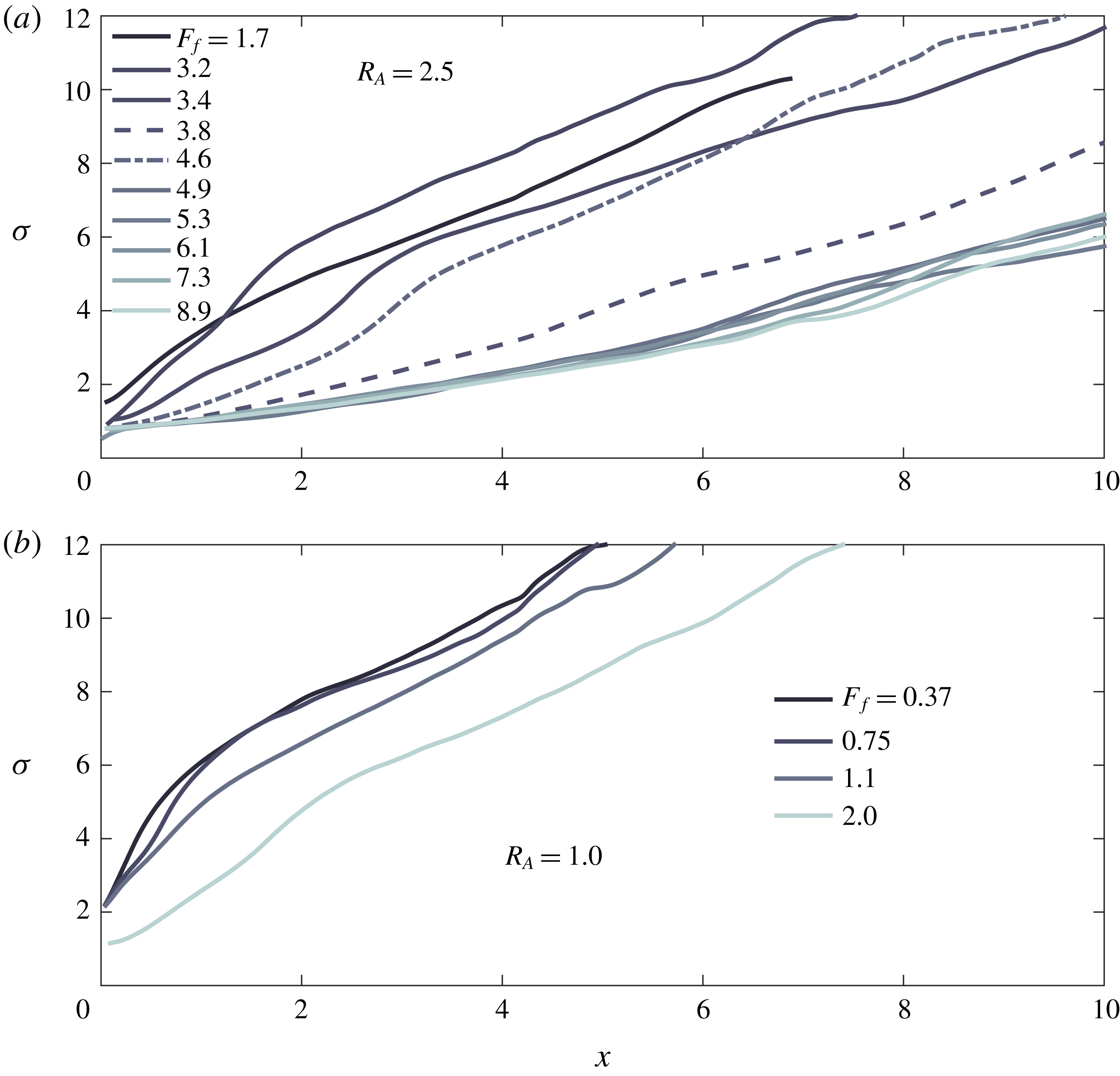
At a lower inflow aspect ratio of
 $R_{A}=1.0$
, we are able to obtain smaller values of the freshwater Froude number and focus on the subcritical and intermediate
 $F_{f}$
regimes (figure 8
b). We see that the two subcritical profiles are convergent and appear to collapse, consistent with the theoretical prediction that the subcritical spreading profile should be essentially independent of
 $F_{f}$
(and truly independent in the limit of an immiscible, inviscid plume). Furthermore, the run corresponding to the highest value of
 $F_{f}$
shows the same transition from divergent to convergent behaviour.
Based on the experimental profiles (figure 8) and the theoretical results shown in figure 4, we propose that the plume profiles may be grouped into three categories: (i) convergent/subcritical (
 $F_{f}\leqslant 1$
), in which the plume is convergent and the spreading behaviour is independent of
 $F_{f}$
; (ii) transitional (
 $1<F_{f}\lesssim 5$
), in which liftoff is pushed offshore, and this expresses itself in the appearance of a length scale defined by the transition in curvature from divergent to convergent plume spreading; and finally (iii) jet-like (
 $F_{f}\gtrsim 5$
), in which the profiles collapse and spreading again becomes independent of
 $F_{f}$
. The transition to jet-like behaviour likely represents the upper limit of the validity of the hydraulic description of the plume. Note that the given value of
 $F_{f}\approx 5$
for transition to jet-like behaviour is based on the value of
 $F_{f}$
for which the profiles appear to be fully independent of the freshwater Froude number and is likely aspect ratio dependent. For example, our results for
 $R_{A}=1.67$
(profiles not shown) indicates a critical value of
 $F_{f}\approx 4$
.
As a last comparison, we have extracted the curvature length scales from the experimental profiles obtained for
 $R_{A}=1.67$
and
 $2.5$
by determining the location of the change in sign of the second derivative of the profiles subject to a moving average filter (figure 9). Two regimes are apparent in the data. In the range
 $1<F_{f}\lesssim 4$
, the curvature length scale appears to be linear in
 $F_{f}$
and only weakly dependent on the aspect ratio (in the range examined). For
 $F_{f}\gtrsim 4$
, there is an abrupt, step-like increase in this length scale. We note that this corresponds to the abrupt transition apparent in the width profiles (figure 8) for
 $R_{A}=2.5$
and
 $4\lesssim F_{f}\lesssim 5$
. We note also that the transition does not occur at precisely the same value of
 $F_{f}$
between runs, as noted above for the experimental profiles (figure 8) and indicated in figure 9 by the fact that the curvature length scale measured for
 $F_{f}=3.8$
exceeds that measured for
 $F_{f}=4.6$
by a factor of approximately two, indicating that the
 $F_{f}=3.8$
run has transitioned to a jet-like behaviour while the
 $F_{f}=4.6$
run has not.
Beyond the transition (
 $F_{f}\gtrsim 5$
), the curvature scale appears to sort more strongly with aspect ratio, and the results for
 $R_{A}=2.5$
suggest that the curvature length saturates as
 $F_{f}$
is increased. This is consistent with the collapse of the profiles seen in figure 8 and further suggests an abrupt transition to a jet-like,
 $F_{f}$
-independent behaviour.
Liftoff length versus
 $F_{f}$
for
 $R_{A}=1.67$
and
 $R_{A}=2.5$
, coloured as indicated in the legend. The points represent experimental measurements of the curvature length associated with transition from divergent to convergent plume spreading, taken as a metric of the liftoff length. The solid curves show liftoff length predicted using the hydraulic theory presented in § 3 and assuming
 $\unicode[STIX]{x1D705}=1$
in (2.2). The shaded red region indicates the apparent transition from plume-like to jet-like spreading, characterized here by an abrupt, almost step-like transition in the curvature length, and the black vertical dashed line indicates where the model predicts that the bottom-attached plume should become barotropically supercritical, in which case no hydraulic solution exists.
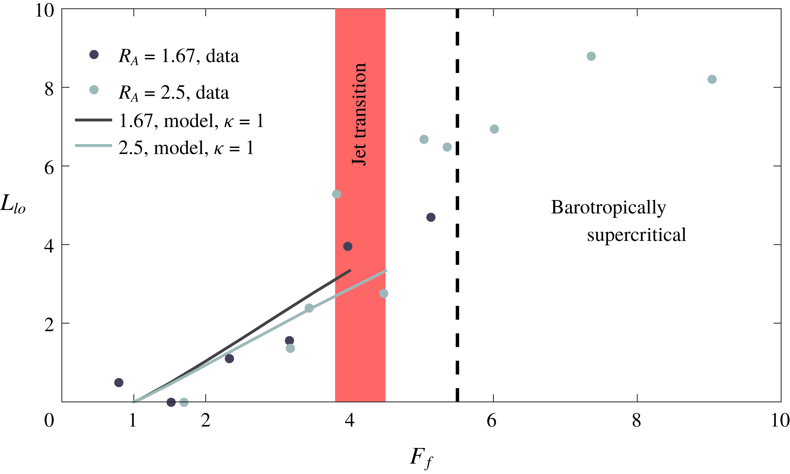
(a) Experimentally measured curvature lengths before the apparent plume-to-jet transition versus
 $F_{f}$
(as in figure 9), along with theoretical predictions for
 $\unicode[STIX]{x1D705}=1$
,
 $0.5$
and
 $0.1$
. Both the experimental data and the theoretical curves are coloured according to
 $R_{A}$
, as indicated in the legend. (b,c) Superelevation at the river mouth (b) and liftoff length (c) versus
 $\unicode[STIX]{x1D705}$
(2.2) for fixed values of
 $F_{f}$
, as indicated in the legend in (c), and a shelf slope
 $\unicode[STIX]{x1D6FC}_{S}=0.003$
. In (a), the shaded region for
 $\unicode[STIX]{x1D705}=1$
indicates the influence of bottom drag and lateral entrainment on the model predictions, with the upper curve corresponding to the inviscid, immiscible solution, and the lower curve corresponding to
 $C_{D}=\unicode[STIX]{x1D6FF}_{L}=10^{-2}$
; the corresponding uncertainty associated with the values of
 $C_{D}$
and
 $\unicode[STIX]{x1D6FF}_{L}$
is similar for the other plotted values of
 $\unicode[STIX]{x1D705}$
and therefore is not shown.
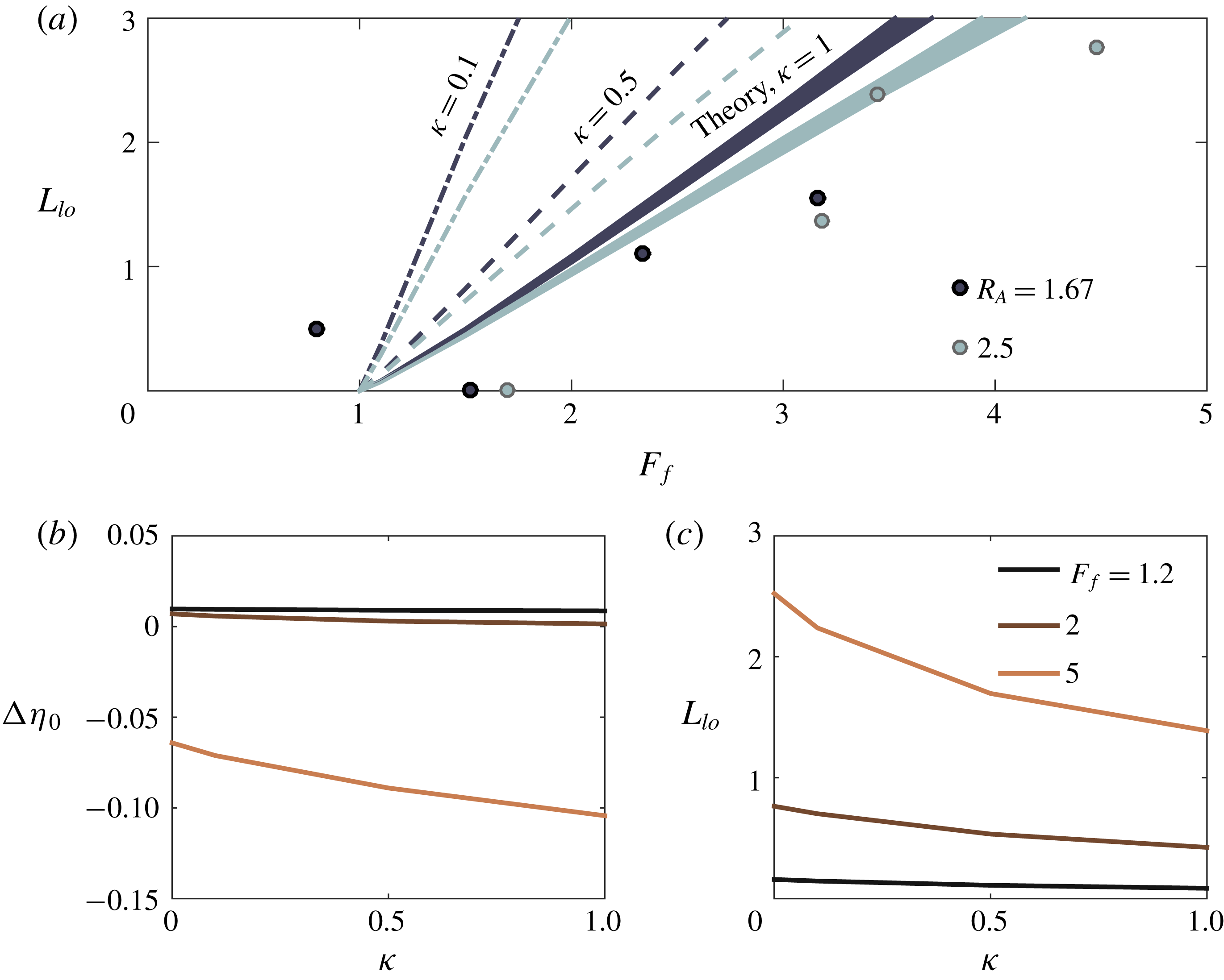
Theoretical prediction of the deviation of the free-surface elevation from sea level,
 $\unicode[STIX]{x0394}\unicode[STIX]{x1D702}\equiv (\unicode[STIX]{x1D702}-h_{S})/h_{S}$
, versus offshore distance. Panel (a) shows
 $\unicode[STIX]{x0394}\unicode[STIX]{x1D702}(x)$
for four subcritical values of
 $F_{f}$
, as indicated in the legend, and
 $\unicode[STIX]{x1D6FC}_{S}=0.003$
. Panel (b) shows
 $\unicode[STIX]{x0394}\unicode[STIX]{x1D702}(x)$
for five supercritical values of
 $F_{f}$
and
 $\unicode[STIX]{x1D6FC}_{S}=0.003$
. Panel (c) shows
 $\unicode[STIX]{x0394}\unicode[STIX]{x1D702}(x)$
for three supercritical values of
 $F_{f}$
and
 $\unicode[STIX]{x1D6FC}_{S}=0$
. In each panel, the thin, colour-coded vertical dot-dashed lines show the location of liftoff for the corresponding value of
 $F_{f}$
, the vertical solid red lines indicate the location of the river mouth, and the dashed blue lines indicate the river slope,
 $\unicode[STIX]{x1D6FC}_{R}=10^{-4}$
. The calculations are performed for
 $R_{A}=250$
,
 $C_{D}=10^{-3}$
, and
 $\unicode[STIX]{x1D705}=1$
.

Theoretical predictions for superelevation at the river mouth
 $\unicode[STIX]{x0394}\unicode[STIX]{x1D702}_{0}\equiv (1-h_{S})/h_{S}$
versus
 $F_{f}$
. Panels (a,c) show the inviscid, immiscible model predictions for three values of
 $R_{A}$
spanning three orders of magnitude (
 $2.5$
,
 $25$
,
 $250$
) and two values of
 $\unicode[STIX]{x1D6FC}_{S}$
:
 $0.05$
(a), the value used in the experiments, and
 $0.003$
(c), a value more typical of what is found in the field. Panel (b) shows the inviscid, immiscible solution (solid line), the immiscible solution with bottom friction (
 $C_{D}=10^{-3}$
, dashed line), and the solution with bottom friction and lateral entrainment (
 $\unicode[STIX]{x1D6FF}_{L}=7\times 10^{-3}$
, dot-dashed line) for
 $R_{A}=25$
and
 $\unicode[STIX]{x1D6FC}_{S}=0.003$
. Panel (d) shows solutions with and without friction and entrainment for a wide estuary and shallow shelf:
 $R_{A}=250$
,
 $\unicode[STIX]{x1D6FC}_{S}=0$
. The inset in (a) shows the same curves as in the main panel but over the range
 $1\leqslant F_{f}\leqslant 2.5$
, a range more relevant to flood conditions likely to be found in the field. For all curves,
 $\unicode[STIX]{x1D705}=1$
.

We also show in figure 9 immiscible and inviscid theoretical predictions for liftoff length, taking
 $\unicode[STIX]{x1D705}=1$
. In figure 10(a), we show only the data before the apparent plume-to-jet transition, along with theoretical predictions for
 $\unicode[STIX]{x1D705}=1$
,
 $0.5$
and
 $0.1$
. The predicted liftoff lengths depend strongly on
 $\unicode[STIX]{x1D705}$
for the
 $O(1)$
aspect ratios accessible in our experiments, and figure 10(a) indicates that the trend in the observed curvature lengths with
 $F_{f}$
is best captured when
 $\unicode[STIX]{x1D705}=1$
, with smaller values of
 $\unicode[STIX]{x1D705}$
greatly over-predicting both the magnitude of the liftoff lengths and the slope of the
 $L_{lo}$
versus
 $F_{f}$
curve. A priori, we expect that the over-prediction of the liftoff length for values of
 $\unicode[STIX]{x1D705}<1$
should be mitigated by the inclusion of bottom friction and the lateral entrainment of momentum, as both result in the deceleration of the plume and thus a more rapid decrease in the local Froude number. However, we find that the predicted liftoff lengths are almost entirely insensitive to the inclusion of bottom drag for
 $C_{D}$
as large as
 $10^{-2}$
and are only weakly dependent on the lateral entrainment coefficient for
 $\unicode[STIX]{x1D6FF}_{L}\leqslant 10^{-2}$
. This is indicated in figure 10(a), where the width of the line corresponding to
 $\unicode[STIX]{x1D705}=1$
indicates the range of predicted liftoff lengths for
 $0\leqslant C_{D}\leqslant 10^{-2}$
and
 $0\leqslant \unicode[STIX]{x1D6FF}_{L}\leqslant 10^{-2}$
; this variation in liftoff length induced by using different values of
 $C_{D}$
and
 $\unicode[STIX]{x1D6FF}_{L}$
is similar irrespective of the value of
 $\unicode[STIX]{x1D705}$
and is therefore shown only for
 $\unicode[STIX]{x1D705}=1$
. Thus, the observed liftoff lengths (figures 9 and 10
a), along with initially divergent shapes of the observed profiles (figure 8) together suggest that the spreading in the bottom-attached plume may be effectively parameterized as
 $\text{d}b/\text{d}x=1/Fr_{1}$
, at least below the plume-to-jet transition (
 $F_{f}\lesssim 4$
). In the model predictions discussed in § 5 below, we therefore perform all calculations with
 $\unicode[STIX]{x1D705}=1$
, unless otherwise noted.
The result that
 $\unicode[STIX]{x1D705}\approx 1$
is surprising. If we conceptualize the bottom-attached plume as spreading laterally as a gravity current, as is done for the surface-trapped plume, this value of
 $\unicode[STIX]{x1D705}$
would require a significant transfer of energy from the along-flow to the lateral direction (Benjamin Reference Benjamin1968), an effect that is not explicitly accounted for in our model. Indeed, given the bidirectional nature of a symmetric lock-exchange flow, we would expect
 $\unicode[STIX]{x1D705}$
to be close to zero (and exactly zero in the limit of an inviscid, immiscible flow). Thus, insofar as our results support of a value of
 $\unicode[STIX]{x1D705}=1$
, this suggests that the spreading dynamics is more complicated than a simple lateral lock exchange. Understanding the mechanisms controlling spreading of the bottom-attached plume is an important direction for future research.
The experimental parameters corresponding to the runs shown in figure 8 are recorded in appendix B, table 3.
5 Hydraulic transitions at the river–ocean interface
The consistency of the theoretical model (§ 3) with the experimental results (§ 4), suggests that the former may be used profitably to predict the structure of the hydraulic transition in the vicinity of the river mouth. We focus on the structure of the free-surface elevation upstream and downstream of the river mouth, examining analytical profiles of the free-surface deviation from sea level:
 $\unicode[STIX]{x0394}\unicode[STIX]{x1D702}\equiv (\unicode[STIX]{x1D702}-h_{S})/h_{S}$
(figure 11). From this, we derive the superelevation at the river mouth, defined as
 $\unicode[STIX]{x0394}\unicode[STIX]{x1D702}_{0}\equiv \unicode[STIX]{x0394}\unicode[STIX]{x1D702}(x=0)\equiv (1-h_{S})/h_{S}$
(figure 12). As discussed above, the superelevation at the river mouth controls the hydraulic structure of the flow upstream of the mouth, which in turn modifies the sediment transport and morphodynamics in the lower river (Chatanantavet et al.
Reference Chatanantavet, Lamb and Nittrouer2012; Lamb et al.
Reference Lamb, Nittrouer, Mohrig and Shaw2012). We further examine analytical predictions for the liftoff length
 $L_{lo}$
(figure 13) and find a simple semi-analytical scaling of
 $L_{lo}$
with
 $F_{f}$
that is anticipated to be valid in natural systems. The location of liftoff is likewise a key parameter controlling sediment transport and morphodynamics in the river–ocean interface. In the first place, it represents a radical shift in sediment dynamics as the flow detaches from the shelf and resuspension is suppressed and depositional rates are consequently enhanced (Kostaschuk et al.
Reference Kostaschuk, Church and Luternauer1992; Geyer Reference Geyer1993; Geyer et al.
Reference Geyer, Hill and Kineke2004; Fugate & Chant Reference Fugate and Chant2005). Secondly, the migration of the liftoff point offshore results in the formation of a depositional bottom-attached plume, possibly contributing to subaqueous canyon formation and delta progradation over geological time scales (Jerolmack Reference Jerolmack2009).
Theoretical predictions for liftoff length
 $L_{lo}$
versus
 $F_{f}$
. Panels (a,c) show the inviscid, immiscible model predictions for three values of
 $R_{A}$
spanning three orders of magnitude (
 $2.5$
,
 $25$
,
 $250$
) and two values of
 $\unicode[STIX]{x1D6FC}_{S}$
:
 $0.05$
(a), and
 $0.003$
(c). Panels (b,d) show solutions with and without friction and entrainment for
 $R_{A}=25$
and
 $\unicode[STIX]{x1D6FC}_{S}=0.003$
(b) and for a wide estuary and shallow shelf:
 $R_{A}=250$
,
 $\unicode[STIX]{x1D6FC}_{S}=0$
(d). The red dashed line in (b) is proportional to
 $F_{f}-1$
. The values of
 $C_{D}$
and
 $\unicode[STIX]{x1D6FF}_{L}$
in (b,d) are as shown in the corresponding panels in figure 12. For all curves,
 $\unicode[STIX]{x1D705}=1$
.

5.1 Free-surface elevation and superelevation at the river mouth
We have used the model to generate profiles of the deviation of the free-surface elevation from sea level, defined as
 $\unicode[STIX]{x0394}\unicode[STIX]{x1D702}\equiv (\unicode[STIX]{x1D702}-h_{S})/h_{S}$
(figure 11). In the subcritical runs, we observe a region in the river (
 $x<0$
) where the free-surface elevation shows essentially no variation (figure 11
a). This corresponds to the salt wedge intrusion, where the surface slope balances the gradual variation of the interfacial elevation and the small interfacial stress. As noted above, we anticipate that the river depth should adjust to the uniform normal depth upstream of the salt wedge intrusion; equivalently, the free-surface slope should approach the river slope (Chow Reference Chow1959). The adjustment to a uniform normal depth far upstream of the salt wedge is indeed confirmed in each of the model runs, although it is difficult to discern in figure 11; this is because the adjustment to normal depth is quite slow, especially when the river is in a backwater state. Indeed, in each of the subcritical profiles we examined, the value of the free-surface slope just upstream of the salt wedge intrusion was less than the river slope, characteristic of a backwater profile.
For each of the subcritical runs, we see that the superelevation is small, less than
 $1\,\%$
of sea level, and always positive (figure 11
a). Further, we note that this superelevation is associated with a rapid decrease in free surface elevation immediately offshore of the mouth (
 $x=0$
) and confined to
 ${\lesssim}5$
channel widths. This is a consequence of the rapid increase in the elevation of the interface downstream of the hydraulic control (figure 3
a,b); in the inviscid, immiscible case, the lower layer momentum equation requires a balance between barotropic and baroclinic pressure gradients (see (A 8)). In dimensioned variables, this is expressed as
 $g\,\text{d}\widetilde{\unicode[STIX]{x1D702}}/\text{d}\widetilde{x}=\text{d}(\widetilde{g}^{\prime }\widetilde{h}_{1})/\text{d}\widetilde{x}$
, indicating that a thinning of the upper layer must be compensated by a decrease in the free-surface elevation, attenuated by a factor
 $g^{\prime }/g\sim \unicode[STIX]{x0394}\unicode[STIX]{x1D70C}_{0}/\unicode[STIX]{x1D70C}_{2}\sim O(0.01)$
. In the subcritical case, when liftoff is in the river channel, the superelevation at the river mouth is set entirely by this mechanism, and
 $\unicode[STIX]{x0394}\unicode[STIX]{x1D702}_{0}$
is consequently necessarily positive and grows with increasing
 $F_{f}$
(figure 11
a).
The superelevation at the river mouth is up to an order of magnitude larger for the supercritical runs, exceeding
 $10\,\%$
of sea level at
 $F_{f}=5$
(figure 11
b). The profiles no longer show a region upstream of the river mouth where the free surface is flat because liftoff has been forced out of the channel and onto the shelf. Further, we observe a transition in the manner in which the free-surface slope approaches the river slope upstream of the river mouth (figure 11
b). For smaller values of
 $F_{f}$
, the evolution of the free-surface elevation is still characteristic of a backwater profile. For larger values of
 $F_{f}$
, there is a transition to a drawdown profile, characterized by decreasing depth, flow acceleration and sediment resuspension/erosion in the downstream direction (Lane Reference Lane1957; Chow Reference Chow1959; Chatanantavet et al.
Reference Chatanantavet, Lamb and Nittrouer2012; Lamb et al.
Reference Lamb, Nittrouer, Mohrig and Shaw2012). The transition from a backwater to a drawdown profile happens for
 $F_{f}\approx 3$
in figure 11(b), but this is strongly a function of the river slope, aspect ratio and bottom drag coefficient. However, in general, the model indicates that transition from backwater to drawdown (and hence in the depositional character of the lower river) happens after liftoff has been forced out of the channel, i.e. for
 $F_{f}>1$
. The combination of flow acceleration and sediment resuspension in the lower river with the formation of a bottom-attached, depositional plume offshore represents a potentially significant source of sediment flux to the coastal ocean during high discharge events, with possible implications for the evolution of the river delta (Jerolmack Reference Jerolmack2009). We note from figure 11(b) that liftoff is confined to within two channel widths of the river mouth for
 $\unicode[STIX]{x1D6FC}_{S}=0.003$
, in contrast to the experimental results (figure 9) and the model results for a flat shelf (figure 11
b), where liftoff is found to extend up to
 ${\sim}8$
channel widths offshore. This suggests a mechanism for the concentrated redistribution of sediment to a region just outside the river mouth during high discharge events, and it is a consequence of the heightened influence of the shelf slope on the thickening of the plume when
 $\unicode[STIX]{x1D6FC}_{S}\neq 0$
and the aspect ratio is large, conditions typical of the field.
Offshore of the river mouth, the supercritical free-surface profiles exhibit a cusp at the liftoff location, corresponding to a discontinuity in the free-surface slope (figure 11
b,c). Although the structure of this cusp is qualitatively similar to what would be seen in a barotropic hydraulic jump, we note that the barotropic Froude number is everywhere less than one in all of the results presented here and no hydraulic jump is present. This cusp is instead the signature of the transition from a bottom-attached plume to a surface-trapped plume and a two-layer flow structure. A bottom-attached plume forms between the river mouth and liftoff in the supercritical runs, and there is a significant free-surface slope in this region. This slope is found to be positive for
 $\unicode[STIX]{x1D6FC}_{S}=0.003$
, a typical field value, for aspect ratios up to
 $R_{A}=250$
(figure 11
b). This can be understood as follows: in the inviscid, immiscible case, the one-layer momentum balance is between the advective acceleration and the barotropic pressure gradient. In dimensioned variables, we have
 $\widetilde{u}\,\text{d}\widetilde{u}/\text{d}\widetilde{x}=-g\,\text{d}\widetilde{\unicode[STIX]{x1D702}}/\text{d}\widetilde{x}$
. The bottom-attached plume is forced to decelerate as it spreads and remains attached to the sloped bottom, and this deceleration is balanced by a positive free-surface slope. Downstream of liftoff, the interfacial height increases rapidly (figure 3
b), and this results in a rapid decrease in the free-surface elevation, as was seen in the subcritical runs downstream of the river mouth. Ultimately, the free surface elevation is constrained to approach sea level asymptotically (
 $\unicode[STIX]{x0394}\unicode[STIX]{x1D702}=0$
), and the superelevation at the river mouth is the net result of the superelevation due to the typically positive free-surface slope in the bottom-attached plume between the river mouth and liftoff and that due to the decrease in free-surface elevation after liftoff. While the peak deviation in free-surface elevation is typically only a few per cent of sea level, it may nonetheless result in a signal that can be detected via airborne or satellite altimetry. Such a signal would provide an opportunity to infer subsurface dynamics and even discharge remotely.
For a typical shelf slope
 $\unicode[STIX]{x1D6FC}_{S}=0.003$
, we find that in the range
 $1<F_{f}\lesssim 2$
, the superelevation due to the decrease in free surface elevation downstream of liftoff exceeds that due to the positive free-surface slope in the bottom-attached plume, resulting in a positive net superelevation at the river mouth (figure 11
b). However, for
 $F_{f}\gtrsim 2$
, the negative superelevation at the river mouth due to the positive free-surface slope in the bottom-attached plume begins to dominate, resulting in a negative superelevation (figure 11
b).
A different behaviour is observed for wide rivers (
 $R_{A}=250$
) discharging into shallow shelves (
 $\unicode[STIX]{x1D6FC}_{S}=0$
) (figure 11
c). In this case, though the free surface slope in the bottom-attached plume is still positive for
 $F_{f}\lesssim 5$
, it is small, and the value of
 $\unicode[STIX]{x0394}\unicode[STIX]{x1D702}_{0}$
is dominated by the decrease in free-surface elevation after liftoff. Furthermore, we find that for
 $F_{f}\gtrsim 5$
the free-surface slope in the bottom-attached plume is negative instead of positive, reinforcing the positive superelevation at the river mouth due to the decrease in free surface elevation after liftoff. In order to understand this result, we solve (2.2) through (3.10) for
 $\text{d}\unicode[STIX]{x1D702}/\text{d}x$
. From this, we find that the sign of the free-surface slope is given by
 $$\begin{eqnarray}\text{sign}\left(\frac{\text{d}\unicode[STIX]{x1D702}}{\text{d}x}\right)=\text{sign}\left[R_{A}(\unicode[STIX]{x1D6FC}_{S}-C_{D})+\frac{h_{1}}{b}\left(\frac{\unicode[STIX]{x1D705}}{Fr_{1}}-4\unicode[STIX]{x1D6FF}_{L}\right)\right].\end{eqnarray}$$
For large aspect ratios and large values of
 $F_{f}$
, the sign of the surface slope is dominated by the first term on the right-hand side. In this case the sign of the initial free-surface slope should be determined by the sign of
 $\unicode[STIX]{x1D6FC}_{S}-C_{D}$
. This is confirmed in figure 11(a,b). Furthermore, even when
 $F_{f}$
is not large enough to suppress the term proportional to
 $1/Fr_{1}$
, the first term is still large and negative, resulting in a free-surface slope in the bottom-attached plume that is only weakly positive and that is dominated by the decrease in free surface elevation after liftoff, leading to a positive superelevation at the river mouth.
These predictions are sensitive to the particular value of
 $\unicode[STIX]{x1D705}$
imposed in the model (2.2). In figure 11, we have performed the calculations with
 $\unicode[STIX]{x1D705}=1$
, as this value was found to best describe the data shown in figure 9. We show in figure 10(b,c) the sensitivity of the predicted superelevation at the river mouth (figure 10
b) and liftoff length (figure 10
b) to
 $\unicode[STIX]{x1D705}\in [0,1]$
for
 $\unicode[STIX]{x1D6FC}_{S}=0.003$
and fixed values of
 $F_{f}=1.2$
,
 $2$
, and
 $5$
. We see that the sensitivity to
 $\unicode[STIX]{x1D705}$
is more pronounced as
 $F_{f}$
increases. In contrast to the pronounced sensitivity of the predicted liftoff length for the laboratory runs shown in figure 9, the field scale (high aspect ratio) predictions for both liftoff length and superelevation are relatively insensitive to
 $\unicode[STIX]{x1D705}$
. This is because, for a large aspect ratio and moderate or large value of
 $\unicode[STIX]{x1D6FC}_{S}$
, the expansion of the plume area, and thus the plume deceleration, is dominated by the vertical expansion induced by the shelf slope. On the other hand, when the shelf is very shallow (as in the flat shelf results shown in figure 11
c) the free-surface structure and the location of liftoff are highly sensitive to
 $\unicode[STIX]{x1D705}$
(figure not shown). Thus, while all of the predictions made here are anticipated to be qualitatively valid, the exact parameter values (
 $R_{A}$
,
 $F_{f}$
) at which transitions in the hydraulic behaviour will occur in the field cannot be predicted with full certainty without a more complete understanding of the processes controlling lateral spreading of the bottom-attached plume.
In order to understand more fully the variation of the superelevation at the river mouth in these different circumstances, we have used the model to generate prediction curves for
 $\unicode[STIX]{x0394}\unicode[STIX]{x1D702}_{0}$
as a function of
 $F_{f}$
up to
 $F_{f}=5.5$
, which is approximately the point when the flow is predicted to become barotropically supercritical (figure 12). The model predictions are calculated in the inviscid, immiscible case and for
 $\unicode[STIX]{x1D705}=1$
. For aspect ratios and bottom slopes typical of natural systems [
 $R_{A}\sim O(10-100)$
,
 $\unicode[STIX]{x1D6FC}_{R}\sim O(0.001)$
], we find that subcritical freshwater Froude numbers consistently result in a small positive superelevation due to the decrease in free-surface elevation at the hydraulic control coincident with the river mouth. The superelevation begins to decrease for
 $F_{f}\geqslant 1$
, and it becomes negative for
 $F_{f}\gtrsim 1.75-2$
(figure 12
a, inset). This is due to the dominance of the positive free-surface slope in the bottom-attached region over the decrease in free-surface elevation after liftoff. At the most extreme, i.e. just before the flow becomes barotropically supercritical (
 $F_{f}=5.5$
), we find that the elevation at the mouth can be as much as
 $20\,\%$
lower than sea level. However, in most natural systems, a freshwater Froude number this large is unlikely to occur (table 1). At a more typical upper limit of
 $F_{f}=2.5$
, the decrease in elevation at the river mouth is
 $O(1\,\%)$
(figure 12
a).
Predictions for
 $\unicode[STIX]{x0394}\unicode[STIX]{x1D702}_{0}$
are relatively insensitive to shelf slope when we compare results computed for the experimental shelf slope (
 $\unicode[STIX]{x1D6FC}_{S}=0.05$
, figure 12
a) and results computed for a slope more typical of natural systems (
 $\unicode[STIX]{x1D6FC}_{S}=0.003$
, figure 12
c). The results also show minimal dependence on aspect ratio, even when
 $R_{A}$
is varied over three orders of magnitude from
 $R_{A}=2.5$
, consistent with our experimental results, to
 $R_{A}=250$
, which represents the upper limit of what can be found in natural systems (table 1, figure 12
a,b). The results are also insensitive to the inclusion of bottom friction and lateral entrainment for
 $\unicode[STIX]{x1D6FC}_{S}=0.003$
and
 $R_{A}=25$
(figure 12
c), and they are typically even less sensitive to bottom friction and lateral entrainment for other combinations of
 $\unicode[STIX]{x1D6FC}_{S}=0.003$
,
 $0.05$
and
 $R_{A}=2.5$
,
 $25$
,
 $250$
(not shown). This is because, for
 $\unicode[STIX]{x1D6FC}_{S}\gg C_{D}$
, the free-surface response in the bottom-attached region is dominated by the gravitational forcing associated with the shelf slope (see (5.1)). The results are no longer insensitive to bottom friction for a wide river (
 $R_{A}=250$
) and shallow shelf (
 $\unicode[STIX]{x1D6FC}_{S}=0$
); as discussed above, both the magnitude and for high
 $F_{f}$
the sign of the initial free-surface slope depends on the sign of
 $\unicode[STIX]{x1D6FC}_{S}-C_{D}$
, and so, when
 $\unicode[STIX]{x1D6FC}_{S}=0$
, introducing a nonzero value of
 $C_{D}$
is enough to change the behaviour of
 $\unicode[STIX]{x0394}\unicode[STIX]{x1D702}_{0}$
from monotonically decreasing to monotonically increasing for
 $F_{f}\geqslant 1$
.
5.2 Liftoff length scaling in the field
Unlike for the superelevation at the mouth, we find that the inviscid, immiscible model predictions for liftoff length are highly sensitive to both shelf slope and aspect ratio (figure 13
a,c). There is an exception to this when
 $\unicode[STIX]{x1D6FC}_{S}=0$
; in this case, the liftoff length is essentially insensitive to the value of
 $R_{A}$
(results not shown). On the other hand, the solution is found to be insensitive to both friction and entrainment even for
 $\unicode[STIX]{x1D6FC}_{S}=0$
, where
 $\unicode[STIX]{x0394}\unicode[STIX]{x1D702}_{0}$
was found to be highly sensitive to the value of
 $C_{D}$
(figure 13
b,d). Although the magnitude of
 $L_{lo}$
is sensitive to the particular value of
 $\unicode[STIX]{x1D6FC}_{S}$
and
 $R_{A}$
, the form of the dependence of
 $L_{lo}$
on
 $F_{f}$
seems to be relatively insensitive to these parameters. We have fit model output for
 $L_{lo}$
versus
 $F_{f}$
for
 $0\leqslant \unicode[STIX]{x1D6FC}_{S}\leqslant 0.5$
and
 $2.5\leqslant R_{A}\leqslant 250$
, both with and without friction and entrainment (figure not shown). Our results indicate that the solution is described very well by scaling of the form (in dimensioned variables)
 $$\begin{eqnarray}\frac{L_{lo}}{b_{0}}=\unicode[STIX]{x1D6FE}(F_{f}-1)^{n}\end{eqnarray}$$
for
 $F_{f}\leqslant 5$
. In this relation,
 $\unicode[STIX]{x1D6FE}$
and
 $n$
are dimensionless geometric constants that vary as functions of
 $R_{A}$
and
 $\unicode[STIX]{x1D6FC}_{S}$
and are fixed for a given system. They are insensitive to the values of
 $C_{D}$
and
 $\unicode[STIX]{x1D6FF}_{L}$
. We find that the exponent
 $n$
falls in the range
 $1\lesssim n\lesssim 1.4$
. Further, for
 $R_{A}\gtrsim 10$
and
 $\unicode[STIX]{x1D6FC}_{S}/C_{D}>1$
,
 $n\approx 1$
and is only weakly sensitive to
 $R_{A}$
and
 $\unicode[STIX]{x1D6FC}_{S}$
. Thus, for intermediate and steep shelf slopes
 $\unicode[STIX]{x1D6FC}_{S}/C_{D}>1$
and aspect ratios
 $R_{A}\gtrsim 10$
, typical of natural systems, our results support the following scaling:
 $$\begin{eqnarray}\frac{L_{lo}}{b_{0}}=\unicode[STIX]{x1D6FE}(F_{f}-1).\end{eqnarray}$$
We find that
 $\unicode[STIX]{x1D6FE}$
decreases with increasing shelf slope, and for natural systems (
 $R_{A}\sim O(10{-}100)$
) it is in the range
 $\unicode[STIX]{x1D6FE}\sim O(10^{-2}-1)$
for
 $0.01\lesssim \unicode[STIX]{x1D6FC}_{S}\lesssim 0.5$
. We thus arrive at a surprisingly simple scaling for the plume liftoff length, given the nonlinearity and relative complexity of the governing hydraulic equations.
6 Conclusions
In this paper, we have presented a unified theoretical framework that may be used to describe the large scale features of the flow in highly stratified estuaries and plumes. In particular, we have extended existing theory by considering the entire river–estuary–plume system as a single dynamically interlinked region (figure 3), by testing the predictions from Poggioli & Horner-Devine (Reference Poggioli and Horner-Devine2015) for intrusion length in a highly stratified estuary with non-zero bottom slope (figure 7), and by extending the theory to the supercritical case, providing a prediction for the dependence of the plume liftoff length on freshwater Froude number (figures 9 and 13). We have also conducted a series of experiments which corroborate our predictions for the interfacial structure of the salt wedge and the spreading profile of the plume, and for the intrusion and liftoff lengths (figures 7, 8, and 9). In doing so, we have also corroborated our conceptual picture of the plume presented in figure 1, and thus provided evidence for our two guiding hypotheses, commonly found in the salt wedge and river plume literature: (i) that the estuary–plume system dynamics is governed by two-layer hydraulics (see, e.g. Hetland Reference Hetland2010), and (ii) that the principal contribution to plume spreading is the buoyant forcing of the plume water, resulting in a spreading rate
 $\text{d}b/\text{d}x\propto Fr_{1}^{-1}$
(see, e.g. Wright & Coleman Reference Wright and Coleman1971; Hetland & MacDonald Reference Hetland and MacDonald2008; Chen et al.
Reference Chen, MacDonald and Hetland2009; Hetland Reference Hetland2010; Yuan & Horner-Devine Reference Yuan and Horner-Devine2013). Furthermore, from both our theoretical and experimental results we have found that the plume may be classified in three dynamic regimes: (i) a subcritical regime (
 $F_{f}\leqslant 1$
), in which the plume width profile is initially convergent, and it is independent of
 $F_{f}$
; (ii) an intermediate regime, characterized by the forcing of the liftoff point further offshore as freshwater Froude number is increased, corresponding to a transition in the plume from divergent to convergent spreading; and finally (iii) a jet-like regime, in which the spreading profiles collapse, again becoming independent of freshwater Froude number, and the dynamics likely transitions from hydraulic flow to dynamics characteristic of a planar turbulent jet.
Finally, we have examined the theoretical predictions for the free-surface structure, superelevation at the river mouth and liftoff length, all of which are anticipated to have an important influence on sediment dynamics across the river–ocean interface and export of sediment to the shelf (figures 11, 12, and 13). We have found that, over the range of freshwater Froude number likely to be encountered in the field, the superelevation is unlikely to have a significant impact on the structure of the hydraulic flow in the river, but that high discharge events may provide a robust signal of the river discharge in the structure of the free surface that is accessible to aerial topography measurements. Furthermore, our results for the liftoff length suggest that, although the governing hydraulic equations are highly nonlinear and relatively complex, the dependence of the liftoff length of freshwater Froude number is surprisingly simple, with
 $L_{lo}/b$
, the liftoff length expressed in channel widths, scaling linearly in
 $F_{f}-1$
, with a geometric prefactor that is anticipated to be roughly constant for a given river system.
Acknowledgements
The authors thank Dr M. P. Lamb for helpful discussions, and J. Neher, N. Johnson, L. England and R. Punt for help with the experiments. This work was funded by National Science Foundation Grant OCE-1233068. A.R.H.-D. is grateful for support from the Allan and Inger Osberg Endowed Professorship.
Appendix A. Derivation of momentum equations
In this appendix we provide a brief recapitulation of the derivation of the equations governing one- and two-layer hydraulic momentum conservation, equations (3.9), (3.10), (3.4), (3.5), (3.6) and (3.7) in the main text.
We assume always that the vertical pressure gradient is dominated by the hydrostatic balance:
 $\unicode[STIX]{x2202}_{\widetilde{z}}\widetilde{p}=-\widetilde{\unicode[STIX]{x1D70C}}g$
. Recall that a tilde indicates a dimensioned independent or dependent model variable. In the case of a single layer, the pressure distribution is
 $$\begin{eqnarray}\widetilde{p}=\widetilde{\unicode[STIX]{x1D70C}}_{1}g(\widetilde{\unicode[STIX]{x1D702}}-\widetilde{z}),\end{eqnarray}$$
and for two layers it is
 $$\begin{eqnarray}\widetilde{p}=\left\{\begin{array}{@{}ll@{}}\widetilde{\unicode[STIX]{x1D70C}}_{1}g(\widetilde{\unicode[STIX]{x1D702}}-\widetilde{z}),\quad & \widetilde{z}\in (\widetilde{\unicode[STIX]{x1D702}}-\widetilde{h}_{1},\widetilde{\unicode[STIX]{x1D702}})\\ \unicode[STIX]{x1D70C}_{2}g(\widetilde{\unicode[STIX]{x1D702}}-\widetilde{z})-\unicode[STIX]{x0394}\widetilde{\unicode[STIX]{x1D70C}}g\widetilde{h}_{1},\quad & \widetilde{z}<\widetilde{\unicode[STIX]{x1D702}}-\widetilde{h}_{1}.\end{array}\right.\end{eqnarray}$$
Thus, we find for the along-flow pressure gradient
 $$\begin{eqnarray}\frac{1}{\widetilde{\unicode[STIX]{x1D70C}}}\frac{\unicode[STIX]{x2202}\widetilde{p}}{\unicode[STIX]{x2202}\widetilde{x}}=g\frac{\text{d}\widetilde{\unicode[STIX]{x1D702}}}{\text{d}\widetilde{x}}+g(\widetilde{\unicode[STIX]{x1D702}}-\widetilde{z})\frac{1}{\widetilde{\unicode[STIX]{x1D70C}}_{1}}\frac{\text{d}\widetilde{\unicode[STIX]{x1D70C}}_{1}}{\text{d}\widetilde{x}}\quad \text{(one layer)}\end{eqnarray}$$
and
 $$\begin{eqnarray}\frac{1}{\widetilde{\unicode[STIX]{x1D70C}}}\frac{\unicode[STIX]{x2202}\widetilde{p}}{\unicode[STIX]{x2202}\widetilde{x}}=\left\{\begin{array}{@{}ll@{}}\displaystyle g\frac{\text{d}\widetilde{\unicode[STIX]{x1D702}}}{\text{d}\widetilde{x}}+g(\widetilde{\unicode[STIX]{x1D702}}-\widetilde{z})\frac{1}{\widetilde{\unicode[STIX]{x1D70C}}_{1}}\frac{\text{d}\widetilde{\unicode[STIX]{x1D70C}}_{1}}{\text{d}\widetilde{x}},\quad & \widetilde{z}\in (\widetilde{\unicode[STIX]{x1D702}}-\widetilde{h}_{1},\widetilde{\unicode[STIX]{x1D702}})\\ \displaystyle g\frac{\text{d}\widetilde{\unicode[STIX]{x1D702}}}{\text{d}\widetilde{x}}-g\frac{\text{d}}{\text{d}\widetilde{x}}(\unicode[STIX]{x0394}\widetilde{\unicode[STIX]{x1D70C}}\widetilde{h}_{1}),\quad & \widetilde{z}<\widetilde{\unicode[STIX]{x1D702}}-\widetilde{h}_{1}\quad \text{(two layers)}.\end{array}\right.\end{eqnarray}$$
The second term on the right-hand side in the one-layer case and in the upper layer in the two-layer case is explicitly depth dependent and difficult to incorporate into our analysis, as we assume all properties are uniform over the layer cross-sections. We will assume that the upper layer is sufficiently thin, and the gradient of the (logarithm of the) upper layer density sufficiently slowly varying that we may neglect this term in comparison to the barotropic pressure gradient,
 $g\,\text{d}\widetilde{\unicode[STIX]{x1D702}}/\text{d}\widetilde{x}$
.
Thus, in the one-layer case, we may immediately write down the one-dimensional
 $x$
-momentum equation, taking into account advection, the pressure gradient, (vertically integrated) stress divergence due to the bottom boundary shear stress, and lateral momentum entrainment. In non-dimensioned variables, we thus have
 $$\begin{eqnarray}u\frac{\text{d}u}{\text{d}x}+\left(\frac{\unicode[STIX]{x0394}\unicode[STIX]{x1D70C}_{0}}{\unicode[STIX]{x1D70C}_{2}}\right)^{-1}\frac{\text{d}\unicode[STIX]{x1D702}}{\text{d}x}=-R_{A}C_{D}\frac{u^{2}}{h_{1}}-2\unicode[STIX]{x1D6FF}_{L}\frac{u^{2}}{b}.\end{eqnarray}$$
We multiply through by
 $\unicode[STIX]{x0394}\unicode[STIX]{x1D70C}_{0}/\unicode[STIX]{x1D70C}_{2}$
and eliminated
 $u$
and
 $\unicode[STIX]{x1D702}$
using respectively freshwater flux conservation (3.1) and the constraint
 $\unicode[STIX]{x1D702}=h_{1}-R_{A}\unicode[STIX]{x1D6FC}x$
:
 $$\begin{eqnarray}\frac{\text{d}}{\text{d}x}\left[\frac{1}{2}\frac{\unicode[STIX]{x0394}\unicode[STIX]{x1D70C}_{0}}{\unicode[STIX]{x1D70C}_{2}}\left(\frac{F_{f}}{b\unicode[STIX]{x0394}\unicode[STIX]{x1D70C}h_{1}}\right)^{2}+h_{1}\right]=R_{A}\unicode[STIX]{x1D6FC}-\frac{\unicode[STIX]{x0394}\unicode[STIX]{x1D70C}_{0}}{\unicode[STIX]{x1D70C}_{2}}\left(R_{A}C_{D}+2\unicode[STIX]{x1D6FF}_{L}\frac{h_{1}}{b}\right)\unicode[STIX]{x0394}\unicode[STIX]{x1D70C}Fr_{1}^{2}.\end{eqnarray}$$
In the case of two layers, we include interfacial but not bottom friction, and we add in the influence of vertical momentum entrainment into the upper layer. We also exclude lateral entrainment flux as it is not meaningful to partition the salt flux across the plume boundary into vertical and lateral components. We thus write for our momentum equations
 $$\begin{eqnarray}u\frac{\text{d}u}{\text{d}x}+\left(\frac{\unicode[STIX]{x0394}\unicode[STIX]{x1D70C}_{0}}{\unicode[STIX]{x1D70C}_{2}}\right)^{-1}\frac{\text{d}\unicode[STIX]{x1D702}}{\text{d}x}=-R_{A}C_{i}\frac{u^{2}}{h_{1}}-R_{A}\unicode[STIX]{x1D6FF}_{V}\frac{u^{2}}{h_{1}}\quad \text{(upper layer)}\end{eqnarray}$$
and
 $$\begin{eqnarray}\left(\frac{\unicode[STIX]{x0394}\unicode[STIX]{x1D70C}_{0}}{\unicode[STIX]{x1D70C}_{2}}\right)^{-1}\frac{\text{d}\unicode[STIX]{x1D702}}{\text{d}x}-\frac{\text{d}}{\text{d}x}(\unicode[STIX]{x0394}\unicode[STIX]{x1D70C}h_{1})=R_{A}C_{i}\frac{u^{2}}{h_{2}}\quad \text{(lower layer)}.\end{eqnarray}$$
We again insert the freshwater flux relation to eliminate
 $u$
, giving
 $$\begin{eqnarray}\frac{\text{d}}{\text{d}x}\left[\frac{1}{2}\left(\frac{F_{f}}{b\unicode[STIX]{x0394}\unicode[STIX]{x1D70C}h_{1}}\right)^{2}+\left(\frac{\unicode[STIX]{x0394}\unicode[STIX]{x1D70C}_{0}}{\unicode[STIX]{x1D70C}_{2}}\right)^{-1}\unicode[STIX]{x1D702}\right]=-R_{A}(C_{i}+\unicode[STIX]{x1D6FF}_{V})\unicode[STIX]{x0394}\unicode[STIX]{x1D70C}Fr_{1}^{2},\end{eqnarray}$$
and
 $$\begin{eqnarray}\frac{\text{d}}{\text{d}x}\left[\left(\frac{\unicode[STIX]{x0394}\unicode[STIX]{x1D70C}_{0}}{\unicode[STIX]{x1D70C}_{2}}\right)^{-1}\unicode[STIX]{x1D702}-\unicode[STIX]{x0394}\unicode[STIX]{x1D70C}h_{1}\right]=R_{A}C_{i}\frac{h_{1}}{h_{2}}\unicode[STIX]{x0394}\unicode[STIX]{x1D70C}Fr_{1}^{2}.\end{eqnarray}$$
We take the difference of (A 9) and (A 10) to eliminate the free-surface elevation, obtaining
 $$\begin{eqnarray}\frac{\text{d}}{\text{d}x}\left[\frac{1}{2}\left(\frac{F_{f}}{b\unicode[STIX]{x0394}\unicode[STIX]{x1D70C}h_{1}}\right)^{2}+\unicode[STIX]{x0394}\unicode[STIX]{x1D70C}h_{1}\right]=-R_{A}\left[C_{i}\left(1+\frac{h_{1}}{h_{2}}\right)+\unicode[STIX]{x1D6FF}_{V}\right]\unicode[STIX]{x0394}\unicode[STIX]{x1D70C}Fr_{1}^{2}.\end{eqnarray}$$
Equation (A 10) is equivalent to (3.5) and (3.7), and (A 11) to (3.4) and (3.6).
Appendix B. Experimental parameters
Experimental parameters for salt wedge runs.
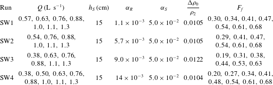
Experimental parameters for plume runs.