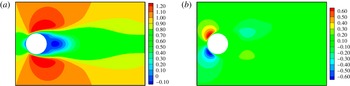
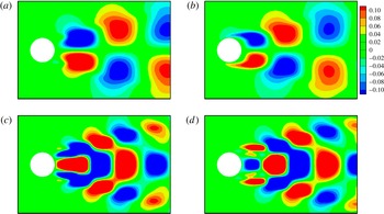
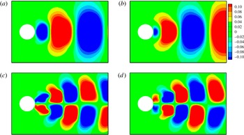
1. Introduction
Control of a flow field has been a subject of interest in recent years. It can lead to significant benefits in engineering and industrial applications. Flow control belongs to the general area of distributed parameter control, and the past decade has seen tremendous advances in both the theory and the application of this field. In recent years, the design of feedback controllers for active control of fluid flows has received considerable attention from the research community (see Sritharan Reference Sritharan1991; Gunzburger Reference Gunzburger1995; Gad-el-Hak Reference Gad-el-Hak1996; Fursikov, Gunzburger & Hou Reference Fursikov, Gunzburger and Hou1998a ,Reference Fursikov, Gunzburger and Hou b ; Sritharan Reference Sritharan1998; Gad-el-Hak Reference Gad-el-Hak2000 and the references therein). Kim & Bewley (Reference Kim and Bewley2007), Bagheri et al. (Reference Bagheri, Henningson, Hoepffner and Schmid2009), Sipp et al. (Reference Sipp, Marquet, Meliga and Barbagallo2010) and Sipp & Schmid (Reference Sipp and Schmid2013) present overviews related to linear control, system identification and model reduction. Recent advances in theory, model reduction and computational tools offer the potential for the development of practical controllers with huge payoffs.
The problem of fluid flow control is modelled by partial differential equations (PDEs), such as Navier–Stokes, Euler, Boussinesq, etc. Physical processes governed by PDEs are infinite-dimensional systems and are typically simulated by numerical methods. However, for a time-varying three-dimensional fluid flow, the spatial degrees of freedom can be of the order of millions, and such computational fluid dynamics (CFD) models are not practical for direct use in control design and optimization of fluid flow systems.
A standard approach to deal with the feedback control problem for PDE models is to discretize the problem or to construct a reduced-order model and then design a control law for the discrete or reduced-order problem. This approach offers the benefit of allowing the designer to use existing finite-dimensional methods to develop the controller. However, unless one constructs the discretized/reduced-order models so that control system properties are preserved, it is known that mesh refinement may not produce convergent feedback control laws (Burns, Ito & Propst Reference Burns, Ito and Propst1988). Moreover, even in the cases where one can establish the convergence of the feedback control law, there are no estimates on how large the controller must be to ensure performance or even stability. Consequently, model reduction is often used as a starting place in order to employ the ‘reduce-then-design’ methodology. This may be a starting point for the computationally intensive ‘design-then-reduce’ approach (Stoyanov Reference Stoyanov2009). Reduced-order modelling of incompressible flows, such as flow past a bluff body, plays an important role in academic and industrial research. Several analytical approaches, such as self-excited oscillator models (Nayfeh et al. Reference Nayfeh, Marzouk, Haider and Akhtar2005; Marzouk et al. Reference Marzouk, Nayfeh, Akhtar and Arafat2007; Akhtar, Marzouk & Nayfeh Reference Akhtar, Marzouk and Nayfeh2009a ), have been proposed to model the vortex shedding. Researchers often use canonical flows to develop reduced-order models and later extend the methods to other complex geometries. Most commonly used is the flow past a circular cylinder.
The proper orthogonal decomposition (POD)-based approach has been applied to various engineering and scientific systems, including modelling of low-dimensional dynamics (Berkooz, Holmes & Lumley Reference Berkooz, Holmes and Lumley1993; Deane & Mavriplis Reference Deane and Mavriplis1994; Holmes, Lumley & Berkooz Reference Holmes, Lumley and Berkooz1996; Ma & Karniadakis Reference Ma and Karniadakis2002; Noack et al. Reference Noack, Afanasiev, Morzynski and Thiele2003), image processing (Holmes et al. Reference Holmes, Lumley and Berkooz1996) and pattern recognition (Sirovich & Kirby Reference Sirovich and Kirby1987). It provides a tool to construct finite-dimensional bases (modes) that optimally represent a dynamical system. These POD bases can be computed from a data set obtained from a numerical simulation or an experiment. Reduced-order models are then constructed by performing a Galerkin projection of the Navier–Stokes equations onto a space spanned by a small number of POD bases. This technique has been applied successfully to grooved channel flows and laminar cylinder wakes (Deane et al. Reference Deane, Kevrekidis, Karniadakis and Orsag1991; Ma & Karniadakis Reference Ma and Karniadakis2002). It should also be noted that, in some cases of POD modes, while optimal in terms of energy representation of a data set, they may not be the best choice for reduced-order modelling (Kim & Bewley Reference Kim and Bewley2007), especially at higher Reynolds numbers. However, recent studies have shown effective use of closure modelling technique to develop reduced-order models for higher Reynolds numbers (Wang et al. Reference Wang, Akhtar, Borggaard and Iliescu2011, Reference Wang, Akhtar, Borggaard and Iliescu2012; Akhtar et al. Reference Akhtar, Wang, Borggaard and Iliescu2012). One of the advantages of POD-based reduced-order models over self-excited oscillator models is that control theory can be applied for flow control design. The placement of sensors (and actuators) in control problems can have a significant impact on the performance and stability of a system. Physical principles are often used to guide the placement in practice, but a number of recent works have introduced a systematic approach to this problem (Fahroo & Demetriou Reference Fahroo and Demetriou2000; Burns et al. Reference Burns, King, Rubio and Zietsman2002; Morris Reference Morris2008).
We consider some recent work that has considerable impact on the control problem. Moreover, we point out some important technical issues that need to be addressed when one considers control problems governed by highly sensitive nonlinear systems with non-normal linearizations. A detailed discussion of these issues along with several illustrative examples may be found in the paper by Burns (Reference Burns, Smith and Demetriou2003). Gillies (Reference Gillies1998) used a neural network approach to provide an empirical prediction of the modal response of the wake to external control forcing. Using a reduced-order model, a closed-loop (CL) control was designed for the flow past a circular cylinder. Cohen et al. (Reference Cohen, Siegal, Wetlesen, Cameron and Sick2004) developed a low-dimensional POD model and used a linear stochastic estimation to map sensor readings of the velocity field on the POD mode coefficients. Their results showed that a five-sensor configuration can keep the root-mean-square estimation error for the amplitudes of the first two modes to within 4 % for the simulation data and within 10 % for the particle image velocimetry (PIV) data. This procedure was developed to determine the number of sensors and their appropriate placement for feedback control suppression of the wake instability. Siegel, Cohen & McLaughlin (Reference Siegel, Cohen and McLaughlin2006) analysed numerically the effect of feedback flow control on the wake of a circular cylinder at a Reynolds number of 100. They based their scheme on a low-dimensional model based on POD. They used linear proportional and differential feedback of the estimated first POD mode. They placed sensors in the wake and actuated the cylinder using its displacement normal to the flow. They reported a 15 % reduction in the drag force and a 90 % reduction in the unsteady lift force. To enable real-time control of synthetic-jet actuated flows, Rediniotis, Ko & Kurdila (Reference Rediniotis, Ko and Kurdila2002) derived a low-dimensional model for the synthetic jet through a Galerkin projection of the Navier–Stokes equations on a POD basis. They discussed controllability of the reduced-order models. They also showed that certain choices of controls, observations and states lead to well conceived controllable systems. Rowley (Reference Rowley2005) demonstrated such cases in which POD-based models are unable to capture the dynamics of the system. He proposed a balanced POD scheme in which the POD snapshot method was used to compute empirical Grammians. Yildirim, Chryssostomidis & Karniadakis (Reference Yildirim, Chryssostomidis and Karniadakis2009) suggested that the extrema of the POD spatial modes are good locations for sensor placement and accurate field reconstruction.
One of the most fundamental issues in developing practical feedback controllers is dealing with the problems of sensor/actuator selection and location. We focus on the problem of sensor location for flow control. However, we note that the ideas presented in this paper apply equally well to the actuator placement problem. We make use of the theory of distributed parameter control to formulate the problem and to develop a practical computational tool for optimal/effective sensor placement when the sensed information is to be used for feedback control.
Although reduced-order models offer considerable benefits in flow simulation and can be used in the ‘reduce-then-design’ approach, direct application of this method does not allow one to use the information contained in the infinite-dimensional feedback law (e.g. the functional gains). In recent years it has been observed that if one first computes the functional gains, then the structure and form of the functional gains can be used in practical control design. The structure of linear feedback laws and the corresponding functional gains can be used to identify good spatial locations for sensors (Burns & King Reference Burns and King1994; Burns, King & Rubio Reference Burns, King and Rubio1998). In particular, the structure of the feedback functional gains provides valuable information about where to place sensors for feedback controllers. If sensors can be placed inside the support (ideally where the magnitude of the functional gains is large), then this location is often (but not always) a good location. If sensors are restricted, then the sensor placement problem must be formulated so that the location is optimal for state estimation. The important point is that the sensor location problem is dependent on several factors including the specific type of controller. The paper by Faulds & King (Reference Faulds and King2000) made use of centroidal Voronoi tessellations to optimally place sensors for linear quadratic Gaussian (LQG) control and applied this to a thermal reactor. In the paper by Burns et al. (Reference Burns, King and Rubio1998) optimal sensor placement is considered for LQG and MinMax controllers and applied to a thermal fluid control problem. In the event that sensors are restricted and state estimation is required, this approach also provides practical (engineering) insight into the design of low-order dynamic controllers (Burns & King Reference Burns and King1998; Atwell & King Reference Atwell and King1999, Reference Atwell and King2004; Atwell, Borggaard & King Reference Atwell, Borggaard and King2001; Pastoor et al. Reference Pastoor, Henning, Noack, King and Tadmor2008; Noack et al. Reference Noack, Schlegel, Morzynski and Tadmor2010; Tadmor et al. Reference Tadmor, Lehmann, Noack, Cordier, Delville, Bonnet and Morzyński2010; Chen & Rowley Reference Chen and Rowley2011; Illingworth, Morgans & Rowley Reference Illingworth, Morgans and Rowley2011; Ma, Ahuja & Rowley Reference Ma, Ahuja and Rowley2011).
One approach is to consider the sensor placement as implementing a quadrature with the functional gain (Burns & King Reference Burns and King1994). Functional gains are the kernels of feedback control operators and arise naturally in the theory of distributed parameter control theory when applied to systems governed by PDEs (Lions Reference Lions1971). If the evolution of a control system is described by a PDE, such as the Navier–Stokes equation on a spatial domain
 ${\it\Omega}\in \mathbb{R}^{3}$
, then all Hilbert–Schmidt linear feedback laws can be represented by an integral operator. In many practical cases there are only a finite number of actuators and hence a finite number of controls, say
 $u_{i}~(i=1,2,\ldots ,P)$
. If the corresponding input operators are continuous, then the standard representation theorem implies that there are functions (the functional gains)
 $\boldsymbol{h}_{i}(\cdot )$
such that
 $$\begin{eqnarray}u_{i}(t)=-\mathscr{K}_{i}\boldsymbol{v}(t,\cdot )=-\int _{{\it\Omega}}\langle \boldsymbol{h}_{i}(x)\boldsymbol{v}(t,x)\rangle \,\text{d}x,\end{eqnarray}$$
where
 $\mathscr{K}_{i}$
is the
 $i$
th row of the gain operator,
 $\boldsymbol{h}_{i}(\cdot )$
is a divergence-free vector field called the functional gain and
 $\boldsymbol{v}(t,\cdot )$
is the solution of the PDE in the spatial domain
 ${\it\Omega}$
.
Functional gains have a number of practical applications in infinite-dimensional control theory; most notable for this paper is their use in actuator/sensor placement. For example, observe that if
 $\boldsymbol{h}_{i}(x)$
is zero outside a region
 ${\it\Omega}_{i}\subset {\it\Omega}$
, then the contribution of the flow field
 $\boldsymbol{v}(t,x)$
in these regions to the control
 $u_{i}(t)$
is zero. We use this information to address the problem of sensor placement.
As noted above, a number of studies have shown that feedback functional gains can be a useful tool for sensor placement studies. However, these prior studies have either been limited to simple linear problems or to mildly nonlinear problems in one dimension. This paper represents the first application of using feedback functional gains for CL sensor placement studies in flow control problems governed by Navier–Stokes equations. Furthermore, we use a mean solution to linearize the flow rather than a steady-state solution often used in the stability analysis (Noack et al. Reference Noack, Afanasiev, Morzynski and Thiele2003). While our computation benefits from the periodic structure of the mean solution, this is not a requirement in the general case. In this paper, we use POD bases for feedback laws to compute functional gains for pole placement rather than gains based on standard linear quadratic regulator (LQR), LQG or MinMax/robust control methods. In fact, we compute functional gains for a pole placement control design for stabilizing the flow using direct output feedback with a small number of strategically placed sensors and without the complexity of building state estimators. The addition of state estimation would only enhance the quality of the feedback design.
The remainder of this paper is organized as follows. In § 2, we discuss a general formulation of the flow control problem. In § 3, we present an overview of the numerical methodology used to simulate the flow past a cylinder. This includes a discussion on the boundary conditions used to model a pair of suction actuators that are used as a control mechanism to suppress the vortex shedding. We solve the incompressible Navier–Stokes equations using a parallel algorithm and collect the flow snapshots of actuated and unactuated flow data to build a reduced-order model. In § 4, we give a brief overview of how we build reduced-order models for these flows. The main features are computing a mean flow, using the POD to develop a low-dimensional basis for the fluctuations of the flow from the mean, and a control function to represent the influence of the actuation on the model. Projection of the Navier–Stokes equations onto this basis leads to a low-dimensional dynamical system for the coefficients of the flow in the basis components. We present an example of the flow past a circular cylinder to demonstrate the accuracy of the reduced-order model. A control design by pole placement is computed. In § 5, we demonstrate that this feedback control can be represented as an integral operator, and the kernel of this operator is the feedback functional gain. The structure of this gain has natural similarities with the reduced basis in which it is expressed. This structure is then used to determine good sensor locations. Natural locations for the sensors correspond to locations where the magnitudes of the functional gain are high. In § 6, we compare two sets of sensor locations. One set corresponds to large magnitudes of the functional gain and the other set corresponds to very small values of the gain. A preliminary validation of the sensor locations shows that the approximation of the feedback operator works well using just four flow measurements, while the same approximation leads to virtually no control when using the same feedback law with a poor set of locations. We conclude this paper with a summary of this study and prospects for future work.
2. Mathematical formulation of the flow control problem
2.1. Problem set-up
In this section, we discuss the general problem of controlling an incompressible viscous fluid in a bounded domain
 ${\it\Omega}\subset \mathbb{R}^{n}$
(
 $n=2$
or 3) by forcing on the boundary
 $\partial {\it\Omega}={\it\Lambda}$
. The system is modelled by the Navier–Stokes equations with Dirichlet boundary control. Let
 $\boldsymbol{w}(t,x)$
,
 $p(t,x)$
and
 ${\it\nu}=1/\mathit{Re}>0$
denote the velocity field, pressure field and kinematic viscosity with the Reynolds number (
 $\mathit{Re}$
) respectively. We consider the controlled Navier–Stokes equations given by
 $$\begin{eqnarray}\displaystyle & \boldsymbol{w}_{t}(t,x)+(\boldsymbol{w}(t,x)\boldsymbol{\cdot }\boldsymbol{{\rm\nabla}})\boldsymbol{w}(t,x)={\it\nu}{\rm\Delta}\boldsymbol{w}(t,x)-\boldsymbol{{\rm\nabla}}p(t,x),\quad x\in {\it\Omega},t>0, & \displaystyle\end{eqnarray}$$
 $$\begin{eqnarray}\displaystyle & \boldsymbol{{\rm\nabla}}\boldsymbol{\cdot }\boldsymbol{w}(t,x)=0,\quad x\in {\it\Omega},t>0, & \displaystyle\end{eqnarray}$$
 $$\begin{eqnarray}\boldsymbol{w}(0,x)=\boldsymbol{w}_{0}(x),\quad x\in {\it\Omega},\end{eqnarray}$$
and controlled boundary condition
 $$\begin{eqnarray}\boldsymbol{w}(t,x)=\boldsymbol{u}(t,x),\quad x\in \partial {\it\Omega}_{c},t>0,\end{eqnarray}$$
with appropriate boundary condition
 $\partial {\it\Omega}\setminus {\it\Omega}_{c}\rightarrow \pm \infty$
. Conservation of mass requires that the boundary control
 $\boldsymbol{u}(t,x)$
satisfy
 $$\begin{eqnarray}\int _{{\it\Lambda}}\boldsymbol{u}(t,x)\boldsymbol{\cdot }\boldsymbol{n}(x)\,\text{d}{\it\Lambda}=0,\end{eqnarray}$$
where
 $\boldsymbol{n}(x)$
is the unit outward normal to the boundary
 ${\it\Lambda}=\partial {\it\Omega}$
. In the problem considered here the control has the form
 $$\begin{eqnarray}\boldsymbol{u}(t,x)=\mathop{\sum }_{i=1}^{P}u_{i}(t){\it\Gamma}_{i}(x),\end{eqnarray}$$
where for each
 $i=1,2,\ldots ,P$
,
 $$\begin{eqnarray}\int _{{\it\Lambda}}{\it\Gamma}_{i}(x)\boldsymbol{\cdot }\boldsymbol{n}(x)\,\text{d}{\it\Lambda}=0,\end{eqnarray}$$
implying the assumption of a divergence-free condition, and hence the control constraint in (2.5) is satisfied automatically. Here,
 ${\it\Gamma}_{i}(x)$
is the spatial distribution of the control modes considered for flow control. Choice of control modes is critical and is discussed in detail in § 4.
A typical strategy for computing feedback control laws for fluids is to linearize the equations about an equilibrium point. For this study, we linearize about a time-averaged flow solution, and the objective of the control is to drive the state to this solution. Let
 $\boldsymbol{W}(x)$
and
 $P(x)$
denote velocity and pressure respectively, corresponding to a time-averaged solution to an uncontrolled problem over the interval
 $[0,T]$
. Then, the pair
 $(\boldsymbol{W}(x),P(x))$
satisfy
 $$\begin{eqnarray}\displaystyle & (\boldsymbol{W}(x)\boldsymbol{\cdot }\boldsymbol{{\rm\nabla}})\boldsymbol{W}(x)={\it\nu}{\rm\Delta}\boldsymbol{W}(x)-\boldsymbol{{\rm\nabla}}P(x)+\boldsymbol{f}(x),\quad x\in {\it\Omega}, & \displaystyle\end{eqnarray}$$
 $$\begin{eqnarray}\displaystyle & \boldsymbol{{\rm\nabla}}\boldsymbol{\cdot }\boldsymbol{W}(x)=0,\quad x\in {\it\Omega}, & \displaystyle\end{eqnarray}$$
 $$\begin{eqnarray}\displaystyle & \boldsymbol{W}(x)=\mathbf{0},\quad x\in \partial {\it\Omega}, & \displaystyle\end{eqnarray}$$
 $$\begin{eqnarray}\boldsymbol{f}(x)=\boldsymbol{w}(0,x)-\boldsymbol{w}(T,x)+\boldsymbol{{\rm\nabla}}\left[\boldsymbol{W}(x)\otimes \boldsymbol{W}(x)-\frac{1}{T}\int _{0}^{T}\boldsymbol{w}(t,x)\otimes \boldsymbol{w}(t,x)\,\text{d}t\right]\end{eqnarray}$$
and
 $\otimes$
represents the Kronecker product. The first two terms vanish for
 $T$
-periodic flows (as in this study), and
 $\boldsymbol{f}$
would vanish altogether for steady state
 $(\boldsymbol{W}(x),P(x))$
. We define the velocity and pressure perturbation fields by
 $\boldsymbol{v}(t,x)=\boldsymbol{w}(t,x)-\boldsymbol{W}(x)$
and
 $q(t,x)=p(t,x)-P(x)$
respectively. The controlled perturbation equation becomes
 $$\begin{eqnarray}\boldsymbol{v}_{t}+(\boldsymbol{v}\boldsymbol{\cdot }\boldsymbol{{\rm\nabla}})\boldsymbol{v}={\it\nu}{\rm\Delta}\boldsymbol{v}-((\boldsymbol{W}\boldsymbol{\cdot }\boldsymbol{{\rm\nabla}})\boldsymbol{v}+(\boldsymbol{v}\boldsymbol{\cdot }\boldsymbol{{\rm\nabla}})\boldsymbol{W})-\boldsymbol{{\rm\nabla}}q-\boldsymbol{f},\quad x\in {\it\Omega},t>0,\end{eqnarray}$$
where
 $$\begin{eqnarray}\displaystyle & \boldsymbol{{\rm\nabla}}\boldsymbol{\cdot }\boldsymbol{v}(t,x)=0,\quad x\in {\it\Omega},t>0, & \displaystyle\end{eqnarray}$$
 $$\begin{eqnarray}\displaystyle & \boldsymbol{v}(0,x)=\boldsymbol{v}_{0}(x),\quad x\in {\it\Omega} & \displaystyle\end{eqnarray}$$
 $$\begin{eqnarray}\boldsymbol{v}(t,x)=\boldsymbol{u}(t,x)=\mathop{\sum }_{i=1}^{P}u_{i}(t){\it\Gamma}_{i}(x),\quad x\in \partial {\it\Omega},t>0.\end{eqnarray}$$
We consider only continuous linear state feedback controllers, so by the Riesz representation theorem each control has the form
 $$\begin{eqnarray}u_{i}(t)=-K_{i}\boldsymbol{v}(t,\cdot )=-\int _{{\it\Omega}}\langle \boldsymbol{h}_{i}(x),\boldsymbol{v}(t,x)\rangle \,\text{d}x,\quad i=1,2,\ldots ,P.\end{eqnarray}$$
The structure of the functional gain provides considerable insight into the spatial nature of the controller. For example, if
 $\boldsymbol{h}_{j}(x)\equiv \mathbf{0}$
in
 ${\it\Omega}$
, then the
 $j$
th controller plays no role in the CL system. More typical is the case where the support of the functional gain is localized or nearly localized. If
 $$\begin{eqnarray}{\it\Omega}_{i}=\text{supp}(\boldsymbol{h}_{i}(\cdot ))=\{x\in {\it\Omega}\boldsymbol{ : }\boldsymbol{h}_{i}(\cdot )\neq \mathbf{0}\}\subset {\it\Omega}\end{eqnarray}$$
denotes the support of the functional gain
 $\boldsymbol{h}_{i}(\cdot )$
, then
 $$\begin{eqnarray}u_{i}(t)=-\int _{{\it\Omega}}\langle \boldsymbol{h}_{i}(x),\boldsymbol{v}(t,x)\rangle \,\text{d}x=-\int _{{\it\Omega}_{i}}\langle \boldsymbol{h}_{i}(x),\boldsymbol{v}(t,x)\rangle \,\text{d}x.\end{eqnarray}$$
Therefore, the only spatial points that contribute to the feedback control law
 $u_{i}(t)$
are points
 $x\in {\it\Omega}_{i}$
, and the only place where one needs sensed or estimated information about the flow is in the region
 ${\it\Omega}_{i}$
. Consequently, once the control law in (2.16) is determined, the corresponding functional gain
 $\boldsymbol{h}_{i}(\cdot )$
provides valuable information about the optimal location of sensors and insight into developing reduced-order controllers based on state estimation techniques such as Kalman filters. We apply this basic idea to the cylinder control problem below. However, we begin with the development of the distributed parameter model so that the rough idea above can be placed on a solid theoretical basis. In addition, this formulation provides the framework to develop rigorous computational algorithms and corresponding reduced-order models for control.
In the present study, we focus on constructing numerical approximations of the PDE feedback control law and the corresponding functional gains. In particular, we use a reduced-order modelling technique developed in Akhtar, Nayfeh & Ribbens (Reference Akhtar, Nayfeh and Ribbens2008) to compute the functional gains. We then analyse these gains to provide insight into the physical behaviour of the feedback control mechanism. The control problem is defined by a flow past a circular cylinder at
 $\mathit{Re}=200$
, and we use suction on the cylinder surface to suppress vortex shedding. It is important to note that the objective of this study is not to design the best controller for the given problem. The main idea presented here is to use simple control laws, compute the associated functional gains, and use them to provide insight into the physical behaviour of the feedback control mechanism.
2.2. A state space formulation
Here, we provide a summary of how one formulates a rigorous distributed parameter state space model for the system of PDEs (2.12)–(2.15) (ignoring
 $\boldsymbol{f}$
for now). Since we are applying a Dirichlet boundary control, a detailed description of the mathematical framework requires the introduction of so-called very weak solutions to the Navier–Stokes equations and lies outside the scope of this paper. However, details may be found in Temam (Reference Temam1997), Sritharan (Reference Sritharan1998), Barbu & Triggiani (Reference Barbu and Triggiani2004), Fursikov (Reference Fursikov2004), Amrouche & Razafison (Reference Amrouche and Razafison2005), Farwig, Galdi & Sohr (Reference Farwig, Galdi and Sohr2005, Reference Farwig, Galdi and Sohr2006a
,Reference Farwig, Galdi and Sohr
b
), Burns (Reference Burns, Gad el Hak and Tsai2006), Barbu, Lasiecka & Triggiani (Reference Barbu, Lasiecka and Triggiani2006), Raymond (Reference Raymond2007a
,Reference Raymond
b
), Amrouche & Rodríguez-Bellido (Reference Amrouche and Rodríguez-Bellido2010) and Raymond & Thevenet (Reference Raymond and Thevenet2010).
Let
 $$\begin{eqnarray}\boldsymbol{H}=\left\{\boldsymbol{v}\in L^{2}({\it\Omega};\mathbb{R}^{n})\text{ such that }\boldsymbol{{\rm\nabla}}\boldsymbol{\cdot }\boldsymbol{v}=0,\text{and}~\boldsymbol{v}\boldsymbol{\cdot }\boldsymbol{n}=0,x\in \partial {\it\Omega}\right\}\end{eqnarray}$$
and
 $$\begin{eqnarray}\boldsymbol{V}=\left\{\boldsymbol{v}\in H^{1}({\it\Omega};\mathbb{R}^{n})\text{ such that }\boldsymbol{{\rm\nabla}}\boldsymbol{\cdot }\boldsymbol{v}=0,\text{and}~\boldsymbol{v}=0,x\in \partial {\it\Omega}\right\}\end{eqnarray}$$
be the typical function spaces of divergent free vector fields, where
 $$\begin{eqnarray}L^{2}({\it\Omega};\mathbb{R}^{n})=\left\{\boldsymbol{v}\boldsymbol{ : }{\it\Omega}\longrightarrow \mathbb{R}^{n}\text{ such that }\int _{{\it\Omega}}\left\Vert \boldsymbol{v}(x)\right\Vert _{\mathbb{ R}^{n}}^{2}\,\text{d}x<+\infty \right\}\end{eqnarray}$$
is the usual Lebesgue space of square integrable vector functions. For
 $r>0$
,
 $H^{r}({\it\Omega};\mathbb{R}^{n})$
is the Sobolev space of vector functions whose distributional derivatives of order up to
 $r$
belong to
 $L^{2}({\it\Omega};\mathbb{R}^{n})$
. If
 $$\begin{eqnarray}\unicode[STIX]{x1D651}=\left\{\boldsymbol{v}\boldsymbol{ : }{\it\Omega}\longrightarrow \mathbb{R}^{n}\text{ such that }\boldsymbol{v}\in C_{0}^{\infty }({\it\Omega}),\boldsymbol{{\rm\nabla}}\boldsymbol{\cdot }\boldsymbol{v}=0\right\},\end{eqnarray}$$
with
 $C_{0}^{\infty }$
the space of infinitely differentiable functions with compact support, then one can show (Sritharan Reference Sritharan1991; Temam Reference Temam2001) that
 $\boldsymbol{H}$
is the closure of
 $\unicode[STIX]{x1D651}$
in
 $L^{2}({\it\Omega};\mathbb{R}^{n})$
and
 $\boldsymbol{V}$
is the closure of
 $\unicode[STIX]{x1D651}$
in
 $H_{0}^{1}({\it\Omega};\mathbb{R}^{n})$
. Let
 $P_{H}:L^{2}({\it\Omega};\mathbb{R}^{n})\longrightarrow \boldsymbol{H}$
be the orthogonal projection onto
 $\boldsymbol{H}$
(the Leray projection) and define the Stokes operator
 $A_{S}:D(A_{S})\subset \boldsymbol{H}\longrightarrow \boldsymbol{H}$
on the domain
 $D(A_{S})=H^{2}({\it\Omega};\mathbb{R}^{n})\cap \boldsymbol{V}$
by
 $$\begin{eqnarray}A_{S}\boldsymbol{v}=P_{H}{\rm\Delta}\boldsymbol{v},\quad \boldsymbol{v}\in D(A_{S}).\end{eqnarray}$$
It follows that the dense and continuous embeddings (Sritharan Reference Sritharan1991)
 $$\begin{eqnarray}D(A_{S})\subset \boldsymbol{V}\subset \boldsymbol{H}=\boldsymbol{H}^{\prime }\subset \boldsymbol{V}^{\prime }\subset [D(A_{S})]^{\prime }\end{eqnarray}$$
are compact, where the prime denotes the dual space. Let
 $A_{0}\boldsymbol{ : }\boldsymbol{V}\longrightarrow \boldsymbol{V}^{\prime }$
be the lifting of
 $A_{S}:D(A_{S})\subset \boldsymbol{H}\longrightarrow \boldsymbol{H}$
to
 $\boldsymbol{V}$
and define the linear operator
 $\mathscr{R}\boldsymbol{ : }\boldsymbol{V}\longrightarrow \boldsymbol{V}^{\prime }$
by
 $$\begin{eqnarray}\mathscr{R}\boldsymbol{v}=-P_{H}((\boldsymbol{W}\boldsymbol{\cdot }\boldsymbol{{\rm\nabla}})\boldsymbol{v}+(\boldsymbol{v}\boldsymbol{\cdot }\boldsymbol{{\rm\nabla}})\boldsymbol{W}).\end{eqnarray}$$
Hence, the Oseen operator
 $A({\it\nu})\boldsymbol{ : }\boldsymbol{V}\longrightarrow \boldsymbol{V}^{\prime }$
given by
 $$\begin{eqnarray}A=A({\it\nu})={\it\nu}A_{0}+\mathscr{R}\end{eqnarray}$$
is the linearized operator corresponding to the velocity–pressure pair
 $(\boldsymbol{W},P)$
given by (2.9). The nonlinear operator
 $F\boldsymbol{ : }\boldsymbol{V}\longrightarrow \boldsymbol{V}^{\prime }$
is defined by
 $$\begin{eqnarray}[F(\boldsymbol{v})]({\it\varphi})=\mathop{\sum }_{i,j=1}^{n}\int _{{\it\Omega}}v_{i}\frac{\partial v_{j}}{\partial x_{i}}{\it\varphi}_{j}\,\text{d}x\end{eqnarray}$$
for each
 ${\it\phi}\in \boldsymbol{V}$
.
In order to complete the model one must define the control input operator. The basic idea is to use the Lions structure (Lions Reference Lions1971). The reader may also refer to Bensoussan et al. (Reference Bensoussan, Da Prato, Delfour and Mitter1992a
,Reference Bensoussan, Da Prato, Delfour and Mitter
b
) and Barbu et al. (Reference Barbu, Lasiecka and Triggiani2006). In particular, one ‘lifts’
 $A\boldsymbol{ : }\boldsymbol{V}\longrightarrow \boldsymbol{V}^{\prime }$
to
 $A_{1}\boldsymbol{ : }\boldsymbol{H}\longrightarrow [D(A^{\ast })]^{\prime }$
by
 $$\begin{eqnarray}A_{1}\boldsymbol{v}=\boldsymbol{w}\quad \text{if and only if}\quad \boldsymbol{w}({\it\varphi})=\langle \boldsymbol{v},A^{\ast }{\it\varphi}\rangle _{\boldsymbol{ H}},\end{eqnarray}$$
where
 $\langle \cdot ,\cdot \rangle _{\boldsymbol{H}}$
is the inner product of the space
 $\boldsymbol{H}$
, and is the
 $L_{2}$
inner product,
 $\langle f,g\rangle _{H}=\int _{{\it\Omega}}\sum _{i=1}^{n}f_{i}(x)g_{i}(x)\,\text{d}x$
, and defines
 $B:L^{2}({\it\Lambda};\mathbb{R}^{n})\longrightarrow [D(A^{\ast })]^{\prime }$
by
 $$\begin{eqnarray}B{\it\Gamma}=-A_{1}D{\it\Gamma},\end{eqnarray}$$
where
 $D$
is the Dirichlet map
 $D:L^{2}({\it\Lambda};\mathbb{R}^{n})\longrightarrow H^{1/2}({\it\Omega};\mathbb{R}^{n})\cap \boldsymbol{H}$
. The state space model for the boundary control problem (2.12)–(2.15) now has the (very) weak formulation
 $$\begin{eqnarray}\frac{\text{d}}{\text{d}t}\boldsymbol{z}(t)=({\it\nu}A_{0}+\mathscr{R})\boldsymbol{z}(t)+F(\boldsymbol{z}(t))+B\boldsymbol{u}(t)-\boldsymbol{f}\in [D(A^{\ast })]^{\prime },\end{eqnarray}$$
where we identify
 $\boldsymbol{z}(t)\in \boldsymbol{H}$
with the vector field
 $\boldsymbol{v}(t,\cdot )$
by
 $$\begin{eqnarray}[\boldsymbol{z}(t)](x)\triangleq \boldsymbol{v}(t,x).\end{eqnarray}$$
The system in (2.30) has some important features that are typical of many flow control problems. It should be noted that although the Stokes operator
 ${\it\nu}A_{0}$
is self-adjoint, the Oseen operator
 $A={\it\nu}A_{0}+\mathscr{R}$
can be highly non-normal if
 $\mathscr{R}\neq 0$
. Therefore, the linearized control system
 $$\begin{eqnarray}\frac{\text{d}}{\text{d}t}\boldsymbol{z}(t)=({\it\nu}A_{0}+\mathscr{R})\boldsymbol{z}(t)+B\boldsymbol{u}(t)-\boldsymbol{f},\quad \boldsymbol{z}(0)=\boldsymbol{z}_{0}\end{eqnarray}$$
can be highly sensitive to parameter variations, initial data and inputs
 $\boldsymbol{u}(\cdot )$
. Computational algorithms for linear control problems with a non-normal
 $A$
operator require special effort. In addition, the nonlinear operator is conservative in the sense that
 $$\begin{eqnarray}\langle F(\boldsymbol{v}),\boldsymbol{v}\rangle _{\boldsymbol{V}}=0,\end{eqnarray}$$
where
 $\langle \cdot ,\cdot \rangle _{\boldsymbol{V}}$
is the inner product of the space
 $\boldsymbol{V}$
; this is the
 $\boldsymbol{H}^{\mathbf{1}}$
inner product
 $\langle f,g\rangle _{\boldsymbol{V}}=\int _{{\it\Omega}}\sum _{i=1}^{n}\sum _{j=1}^{n}((\partial f_{i}(x)/\partial x_{j})(\partial g_{i}(x)/\partial x_{j}))\,\text{d}x$
for all
 $\boldsymbol{v}\in \boldsymbol{V}$
, and this special structure tends to be highly sensitive to disturbances (Burns Reference Burns, Smith and Demetriou2003). Sensitivity and non-normality of the linear system lead to many difficulties in the corresponding control problem.
2.3. A feedback control problem
We now consider the feedback control problems for the Navier–Stokes system
 $$\begin{eqnarray}\frac{\text{d}}{\text{d}t}\boldsymbol{z}(t)=A\boldsymbol{z}(t)+F(\boldsymbol{z}(t))+B\boldsymbol{u}(t)-\boldsymbol{f}\end{eqnarray}$$
and the corresponding linearized system
 $$\begin{eqnarray}\frac{\text{d}}{\text{d}t}\boldsymbol{z}(t)=A\boldsymbol{z}(t)+B\boldsymbol{u}(t)-\boldsymbol{f},\end{eqnarray}$$
where again
 ${\it\nu}=1/\mathit{Re}$
and
 $A={\it\nu}A_{0}+\mathscr{R}$
.
New theoretical results on boundary feedback control for the Navier–Stokes equations in 2D and 3D have set the stage for implementation of practical controllers and computational approximations. The LQR approach was applied to tangential boundary control in Barbu & Triggiani (Reference Barbu and Triggiani2004) and Barbu et al. (Reference Barbu, Lasiecka and Triggiani2006) and for more general boundary control in Raymond (Reference Raymond2007a ,Reference Raymond b ) and Raymond & Thevenet (Reference Raymond and Thevenet2010). These papers provide conditions for stabilizability of the linearized and nonlinear equations.
It is important to note that there are many ‘feedback control problems’ (linear feedback, nonlinear feedback, LQR, LQG,
 $H^{\infty }$
, MinMax, pole placement, etc.) and several technical approaches to each of these problems. The LQR, LQG and MinMax approaches have been applied in other flow control problems (Burns et al.
Reference Burns, King and Rubio1998; Fursikov et al.
Reference Fursikov, Gunzburger and Hou1998a
; Burns Reference Burns, Smith and Demetriou2003, Reference Burns, Gad el Hak and Tsai2006; Hogberg, Bewley & Henningson Reference Hogberg, Bewley and Henningson2003; Fursikov, Gunzburger & Hou Reference Fursikov, Gunzburger and Hou2005).
We focus on pole placement as another example to illustrate the point that the particular control design method is not the critical issue in the sensor placement problem. What we do here could have been done using any of the previous methods. The problem of interest is to find a feedback controller that stabilizes the flow and then use the structure of the controller to find good sensor/actuator locations. The only assumption we make here is that the linearized Navier–Stokes system (2.35) is stabilizable so that there is a continuous linear feedback gain operator
 $$\begin{eqnarray}\mathscr{K}:D(\mathscr{K})\subseteq \boldsymbol{H}\longrightarrow \boldsymbol{U}=\mathbb{R}^{m},\end{eqnarray}$$
such that the CL operator
 $$\begin{eqnarray}A_{CL}({\it\nu})\triangleq A({\it\nu})-B\mathscr{K}=({\it\nu}A_{0}+\mathscr{R}-B\mathscr{K})\end{eqnarray}$$
generates a semigroup
 $S_{CL}(t,{\it\nu})=\text{e}^{A_{CL}({\it\nu})t}$
satisfying
 $$\begin{eqnarray}\Vert S_{CL}(t,{\it\nu})\Vert _{\boldsymbol{H}}\leqslant Q\text{e}^{-{\it\beta}t},\end{eqnarray}$$
for some
 $Q\geqslant 1$
and
 ${\it\beta}>0$
. It is important to note that if
 $Q>1$
, then the corresponding CL nonlinear Navier–Stokes equations
 $$\begin{eqnarray}\frac{\text{d}}{\text{d}t}\boldsymbol{z}(t)=({\it\nu}A_{0}+\mathscr{R}-B\mathscr{K})\boldsymbol{z}(t)+F(\boldsymbol{z}(t))\end{eqnarray}$$
may not be exponentially asymptotically stable. However, if
 $Q=1$
, then one can show that the CL nonlinear Navier–Stokes system is exponentially asymptotically stable. Achievement of a CL asymptotically stable system is possible in 3D nonlinear flows with linear feedback even when the Reynolds number is greater than the critical Reynolds number. Fursikov (Reference Fursikov2004) and Burns (Reference Burns, Gad el Hak and Tsai2006) have results along this line. Moreover, in the case with control along the entire boundary, Barbu et al. (Reference Barbu, Lasiecka and Triggiani2006) have proven the existence of a linear feedback operator
 $\mathscr{K}:H^{1/2+{\it\varepsilon}}({\it\Omega};\mathbb{R}^{n})\cap \boldsymbol{H}\longrightarrow \boldsymbol{U}=L^{2}({\it\Lambda};\mathbb{R}^{n})$
for any small
 ${\it\varepsilon}>0$
, such that the nonlinear CL Navier–Stokes equation (2.39) is exponentially asymptotically stable. Furthermore, this feedback gain operator can be computed by solving an abstract Riccati operator equation.
For the problem considered in this paper with a finite number of controllers, the assumption that the system (2.35) is stabilizable with
 $\mathscr{K}:D(\mathscr{K})\subseteq \boldsymbol{H}\longrightarrow \mathbb{R}^{m}$
continuous implies (Riesz representation theorem) that there exist divergent free vector fields
 $\boldsymbol{h}_{i}(\cdot )\in \boldsymbol{H},i=1,2,\ldots ,P$
, so that
 $$\begin{eqnarray}\boldsymbol{u}(t)=\left[\begin{array}{@{}c@{}}u_{1}(t)\\ u_{2}(t)\\ \vdots \\ u_{P}(t)\end{array}\right]=-\mathscr{K}\boldsymbol{v}(t)=-\left[\begin{array}{@{}c@{}}\displaystyle \int _{{\it\Omega}}\langle \boldsymbol{h}_{1}(x),\boldsymbol{v}(t,x)\rangle \,\text{d}x\\ \displaystyle \int _{{\it\Omega}}\langle \boldsymbol{h}_{2}(x),\boldsymbol{v}(t,x)\rangle \,\text{d}x\\ \vdots \\ \displaystyle \int _{{\it\Omega}}\langle \boldsymbol{h}_{P}(x),\boldsymbol{v}(t,x)\rangle \,\text{d}x\end{array}\right],\end{eqnarray}$$
where the functions
 $\boldsymbol{h}_{i}(\cdot )$
are called the feedback functional gains. As noted above, we shall use the spatial information contained in the support of these functional gains to address the sensor placement problem (Burns et al.
Reference Burns, King and Rubio1998).
In this study, we will use pole placement as a design methodology, thus it is important to know that the spectrum of the CL operator determines the stability of the CL system. When
 ${\it\Omega}$
is smooth and bounded, much is known about the spectrum of the linearized Oseen operator
 $A={\it\nu}A_{0}+\mathscr{R}$
and the stability of the linearized problem. The following result follows from Theorem 3.6 in Sritharan (Reference Sritharan1991).
Theorem 1. If
 ${\it\Omega}$
is bounded with smooth boundary, then the Oseen operator
 $A={\it\nu}A_{0}+\mathscr{R}$
has compact resolvent and generates an analytic semigroup on
 $\boldsymbol{H}$
. The spectrum of
 $A$
is only a point spectrum (i.e.
 ${\it\sigma}(A)={\it\sigma}_{p}(A)$
), the eigenvalues all have finite geometric multiplicity, accumulate only at
 $-\infty$
and there are at most a finite number of eigenvalues
 ${\it\lambda}_{i},i=1,2,\ldots ,q$
, satisfying
 $\mathit{Re}({\it\lambda}_{i})\geqslant 0$
.
Theorem 1 implies that in order to stabilize the linearized flow one needs only to ‘move’ a finite number of eigenvalues to the left half of the complex plane. This fact is the basis of much of the work in the paper by Barbu & Triggiani (Reference Barbu and Triggiani2004) and has been extended to boundary control in Barbu et al. (Reference Barbu, Lasiecka and Triggiani2006).
It should be noted that when linearizing about a mean flow, the term
 $-\boldsymbol{f}$
in (2.35) can be treated by finding a solution to the Oseen equations
 $({\it\nu}A_{0}+\mathscr{R})\boldsymbol{g}=\boldsymbol{f}$
. A substitution
 $\boldsymbol{y}=\boldsymbol{z}-\boldsymbol{g}$
produces the standard homogeneous control problem. Applying the feedback control
 $-\mathscr{K}\boldsymbol{y}$
to the homogeneous problem is equivalent to applying
 $\boldsymbol{u}(t)=-\mathscr{K}\boldsymbol{z}(t)+\mathscr{K}\boldsymbol{g}$
, where the last term applies a DC shift to the feedback control.
3. Numerical simulations
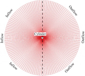
We solve the governing equations by employing
 $192\times 256$
grid points in the radial (
 $r$
) and circumferential (
 ${\it\theta}$
) directions respectively, with an outer diameter of
 $50d$
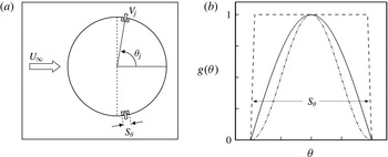
. We employ no-slip and no-penetration boundary conditions on the cylinder surface. However, the boundary conditions can be modified to simulate other flow configurations, such as the case of a cylinder rotating along its axial direction. We can also enforce a fixed or time-varying velocity boundary condition (
 $V_{j}$
) to simulate suction/blowing on the surface to perturb the flow field in the near vicinity of the cylinder for control purposes. In this study, only suction is used as the flow control mechanism. Details of the numerical methods and modelling of boundary conditions on the cylinder surface are given in appendix A.
3.1. Proper orthogonal decomposition
Here, we present a general procedure to compute the POD modes used in this study. The velocity data
 $\boldsymbol{v}=(v_{1},v_{2})$
are then recorded over a shedding cycle, commonly referred to as snapshots in the POD community. The data are assembled in a matrix
 $\unicode[STIX]{x1D652}$
of the form
 $$\begin{eqnarray}\unicode[STIX]{x1D652}=\left[\begin{array}{@{}cccc@{}}v_{11}^{(1)} & v_{11}^{(2)} & \cdots \, & v_{11}^{(S)}\\ \vdots & \vdots & & \vdots \\ v_{1N}^{(1)} & v_{1N}^{(2)} & \cdots \, & v_{1N}^{(S)}\\ v_{21}^{(1)} & v_{21}^{(2)} & \cdots \, & v_{21}^{(S)}\\ \vdots & \vdots & & \vdots \\ v_{2N}^{(1)} & v_{2N}^{(2)} & \cdots \, & v_{2N}^{(S)}\end{array}\right]_{2N\times S},\end{eqnarray}$$
where
 $N$
is the number of grid points and
 $S$
is the number of snapshots taken at constant intervals. We note that the mean velocity field is subtracted from the
 $\unicode[STIX]{x1D652}$
matrix prior to computing the POD modes.
We perform a singular-value decomposition (SVD) of the ensemble data to compute the POD eigenfunctions, that is,
 $\unicode[STIX]{x1D652}={\it\Phi}{\it\Sigma}\unicode[STIX]{x1D651}^{\text{T}}$
, where
 ${\it\Phi}$
represents the POD eigenfunctions,
 ${\it\Sigma}$
contains the singular values
 ${\it\sigma}_{i}$
and
 $\unicode[STIX]{x1D651}$
is the matrix of right singular vectors. We compute the first
 $S$
POD modes using standard LAPACK routines. An important property of these eigenfunctions is orthogonality; that is,
 ${\it\Phi}_{i}\cdot {\it\Phi}_{j}={\it\delta}_{ij}$
, where
 ${\it\delta}_{ij}$
is the Kronecker delta. The optimality of the POD eigenfunction lies in capturing the greatest possible fraction of the total kinetic energy for a projection of the snapshot data onto a fixed number of basis functions. The eigenvalue
 ${\it\lambda}_{i}$
of
 $\unicode[STIX]{x1D652}^{\text{T}}\unicode[STIX]{x1D652}$
is a measure of the energy represented by the
 $i$
th eigenfunction and is equal to the square of the corresponding singular value
 ${\it\sigma}_{i}$
. Since the exterior flow problem is solved in a large domain, the standard
 $L_{2}$
inner product would place a significant emphasis on the outer region of the domain. To accurately capture the physics near the cylinder, we use a weighted
 $L_{2}$
inner product for both creating the basis functions and computing the reduced-order model. The weight function we use is motivated by the radial clustering of points towards the cylinder and is given as
 $$\begin{eqnarray}w(r)=\frac{1}{(r-a)(\text{e}^{{\it\kappa}/192}-1)},\quad \text{for}~{\it\kappa}=\ln \left(\frac{50-a}{b}\right)\!,a=0.3~\text{and}~b=0.2.\end{eqnarray}$$
3.2. Simulation cases
We simulate the flow past the cylinder at
 $\mathit{Re}=200$
for long enough to reach the periodic state. We note that, although the flow field at this Reynolds number is three-dimensional after the mode-A instability (Williamson Reference Williamson1996) at
 $\mathit{Re}\approx 180$
, we consider a two-dimensional flow at this Reynolds number to demonstrate the flow control strategy and sensor placement technique developed in this paper. We consider two simulation cases, with and without boundary control.
3.2.1. Case I: no control
We simulate the flow past the cylinder without control (unactuated), i.e. no-slip no-penetration (homogeneous) velocity boundary conditions on the cylinder surface. The flow field data are recorded in the matrix termed as
 $\unicode[STIX]{x1D652}^{una}$
. In the present case, we sample
 $S=40$
snapshots over one shedding cycle in the periodic flow with a constant time interval (
 ${\rm\Delta}T_{s}$
). We then compute the mean velocity field
 $\bar{\boldsymbol{v}}_{una}$
from
 $\unicode[STIX]{x1D652}^{una}$
and plot the components in figure 1.
Average flow fields at
 $\mathit{Re}=200$
. (a) Streamwise mean velocity. (b) Cross-flow mean velocity.

3.2.2. Case II: suction control
The control mechanism adopted in this study is through modelling a pair of suction actuators by modifying the velocity boundary condition on the cylinder surface. The suction actuators are placed symmetrically about the streamwise direction at
 $\pm 80^{\circ }$
, motivated by the study of Akhtar et al. (Reference Akhtar, Nayfeh and Ribbens2008) in which they used the pressure POD distribution of the most dominant mode on the cylinder surface (see appendix A and figure 19). We perform a simulation with similar flow conditions until a steady state is achieved. We then introduce a suction control with a jet velocity of
 $0.3U_{\infty }$
on the cylinder surface. The flow field is perturbed, reducing the strength of vortex shedding. The velocity data are then recorded for a shedding cycle with
 $S=40$
in the
 $\unicode[STIX]{x1D652}$
matrix and are termed as
 $\unicode[STIX]{x1D652}^{act}$
. We again compute the mean velocity field
 $\bar{\boldsymbol{v}}_{act}$
from
 $\unicode[STIX]{x1D652}^{act}$
. We note that
 $\bar{v}_{act}$
has a non-homogeneous velocity boundary condition on the cylinder surface where suction actuators are modelled.
4. Reduced-order model
In this section, we present the procedure for developing a reduced-order model of the actuated flow field. This includes a brief discussion of the control function method used to include control actuation in the model. For details, readers are referred to the work of Graham, Peraire & Tang (Reference Graham, Peraire and Tang1999).
4.1. The control function approach
A conventional velocity expansion in POD-based reduced-order models is given by
 $$\begin{eqnarray}\boldsymbol{v}(x,t)\approx \bar{\boldsymbol{v}}(x)+\mathop{\sum }_{i=1}^{M}z_{i}^{r}(t){\it\Phi}_{i}(x),\end{eqnarray}$$
where the
 $z_{i}^{r}(t)$
is the temporal coefficient of the
 $i$
th POD mode for the reduced-order model. However, the velocity expansion in (4.1) is not a valid candidate in the Galerkin projection, as it does not automatically satisfy the boundary conditions for arbitrary values of
 $z_{i}^{r}$
.
The control function approach is motivated by requiring homogeneous boundary conditions on the basis functions used in the Galerkin projection. The homogeneous boundary condition is maintained by introducing a suitable function in the velocity expansion, known as the ‘control function’.
Following Graham et al. (Reference Graham, Peraire and Tang1999), we remove the inhomogeneous boundary condition on the cylinder surface by subtracting a suitable ‘control function’ from each snapshot before generating the POD basis functions. We generate the control function by subtracting the mean velocity obtained in case I from that of case II as
 $$\begin{eqnarray}{\it\Gamma}(x)=\bar{\boldsymbol{v}}(x)_{act}-\bar{\boldsymbol{v}}(x)_{una},\quad x\in {\it\Omega}.\end{eqnarray}$$
Thus, the modified snapshot matrix
 $\unicode[STIX]{x1D652}^{mod}$
is now given as
 $$\begin{eqnarray}\unicode[STIX]{x1D652}^{mod}=\unicode[STIX]{x1D652}^{act}-u(t^{k}){\it\Gamma}(x),\end{eqnarray}$$
where
 $u$
corresponds to the variable control input, suction in the present study, kept constant in case II specifically for this purpose. The mean flow and basis functions (
 ${\it\Phi}_{i}$
) are obtained from
 $\unicode[STIX]{x1D652}^{mod}$
as described in § 3.1. The
 ${\it\Phi}_{i}$
maintain their properties with zero velocity on the cylinder surface.
4.2. The model
The velocity expansion now includes the control function and is modified as
 $$\begin{eqnarray}\boldsymbol{v}(x,t)\approx \bar{\boldsymbol{v}}(x)+\mathop{\sum }_{i=1}^{M}z_{i}^{r}(t){\it\Phi}_{i}(x)+u(t){\it\Gamma}(x).\end{eqnarray}$$
For the general procedure with
 $P$
control inputs, the reduced-order model is developed in appendix B. However, in the main text of this paper, we present the reduced-order model for a single control input as expressed in (4.4). We substitute (4.4) into (2.12), identifying
 $\boldsymbol{W}$
with
 $\bar{\boldsymbol{v}}$
, project these equations along the
 ${\it\Phi}_{k}$
, eliminating the pressure perturbation
 $q$
, and obtain
 $$\begin{eqnarray}\dot{\boldsymbol{z}}^{r}=\boldsymbol{A}_{1}^{r}+\boldsymbol{A}_{2}^{r}\boldsymbol{z}^{r}+\boldsymbol{A}_{3}^{r}u+\boldsymbol{F}_{1}^{r}(\boldsymbol{z}^{r})\boldsymbol{z}^{r}+\boldsymbol{F}_{2}^{r}(\boldsymbol{z}^{r})u+\boldsymbol{F}_{3}^{r}(u)u+\boldsymbol{B}^{r}\dot{u},\end{eqnarray}$$
where the operators are represented by
 $$\begin{eqnarray}\displaystyle & \displaystyle [\boldsymbol{A}_{1}^{r}]_{k}=\frac{1}{\mathit{Re}}\langle {\it\Phi}_{k},{\it\Delta}^{h}\bar{\boldsymbol{v}}\rangle -\langle {\it\Phi}_{k},\bar{\boldsymbol{v}}\boldsymbol{\cdot }{\rm\nabla}^{h}\bar{\boldsymbol{v}}\rangle , & \displaystyle\end{eqnarray}$$
 $$\begin{eqnarray}\displaystyle & \displaystyle [\boldsymbol{A}_{2}^{r}]_{km}=-\langle {\it\Phi}_{k},\bar{\boldsymbol{v}}\boldsymbol{\cdot }{\rm\nabla}^{h}{\it\Phi}_{m}\rangle -\langle {\it\Phi}_{k},{\it\Phi}_{m}\boldsymbol{\cdot }{\rm\nabla}^{h}\bar{\boldsymbol{v}}\rangle +\frac{1}{\mathit{Re}}\langle {\it\Phi}_{k},{\it\Delta}^{h}{\it\Phi}_{m}\rangle , & \displaystyle\end{eqnarray}$$
 $$\begin{eqnarray}\displaystyle & \displaystyle [\boldsymbol{A}_{3}^{r}]_{k}=-\langle {\it\Phi}_{k},\bar{\boldsymbol{v}}\boldsymbol{\cdot }{\rm\nabla}^{h}{\it\Gamma}\rangle -\langle {\it\Phi}_{k},{\it\Gamma}\boldsymbol{\cdot }{\rm\nabla}^{h}\bar{\boldsymbol{v}}\rangle +\frac{1}{\mathit{Re}}\langle {\it\Phi}_{k},{\it\Delta}^{h}{\it\Gamma}\rangle , & \displaystyle\end{eqnarray}$$
 $$\begin{eqnarray}\displaystyle & [\boldsymbol{F}_{1}^{r}]_{kmn}=-\langle {\it\Phi}_{k},{\it\Phi}_{m}\cdot {\rm\nabla}^{h}{\it\Phi}_{n}\rangle , & \displaystyle\end{eqnarray}$$
 $$\begin{eqnarray}\displaystyle & [\boldsymbol{F}_{2}^{r}]_{km}=-\langle {\it\Phi}_{k},{\it\Gamma}\cdot {\rm\nabla}^{h}{\it\Phi}_{m}\rangle -\langle {\it\Phi}_{k},{\it\Phi}_{m}\cdot {\rm\nabla}^{h}{\it\Gamma}\rangle , & \displaystyle\end{eqnarray}$$
 $$\begin{eqnarray}\displaystyle & [\boldsymbol{F}_{3}^{r}]_{k}=-\langle {\it\Phi}_{k},{\it\Gamma}\cdot {\rm\nabla}^{h}{\it\Gamma}\rangle , & \displaystyle\end{eqnarray}$$
 $$\begin{eqnarray}\displaystyle & [\boldsymbol{B}^{r}]_{k}=-\langle {\it\Phi}_{k},{\it\Gamma}\rangle , & \displaystyle\end{eqnarray}$$
 $k,m,n=1,2,\ldots ,M$
and where
 $\langle \cdot ,\cdot \rangle$
is the Euclidean inner product.
To validate the reduced-order model developed here, we consider the unactuated case, i.e. case I. Only for this section, we use the
 $\unicode[STIX]{x1D652}^{una}$
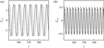
matrix to compute the mean velocity field (see figure 1) and the first 12 POD modes after mean subtraction. We integrate (4.5), with
 $u=0$
, to compute the coefficients
 $z_{i}^{r}$
and plot them in figure 2. The first pair of time coefficients corresponds to the shedding frequency while the second pair is its harmonic. We also observe a phase shift between the states within a pair. We then project each snapshot onto the POD modes to compute the velocity coefficient
 $\tilde{z}_{i}(t)$
as follows:
 $$\begin{eqnarray}\tilde{z}_{i}(t)=\langle \boldsymbol{v}^{\prime }(x,t_{i}),{\it\Phi}(x)\rangle _{\boldsymbol{H}}.\end{eqnarray}$$
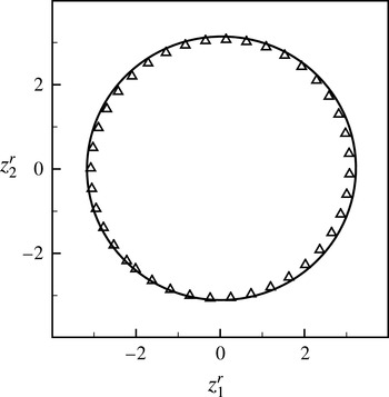
For the 12-dimensional Galerkin model, we investigate the two-dimensional projection of the phase portrait onto the plane (
 $z_{1}^{r},z_{2}^{r}$
) and compare it with the two-dimensional projection onto the plane (
 $\tilde{z}_{1},\tilde{z}_{2}$
) obtained using (4.13). We observe that the two projections compare well, as shown in figure 3.
The velocity coefficients
 $z_{i}^{r},i=1,2,3,4$
, at
 $\mathit{Re}=200$
: (a)
 $z_{1}^{r}$
(solid) and
 $z_{2}^{r}$
(dashed); (b)
 $z_{3}^{r}$
(solid) and
 $z_{4}^{r}$
(dashed).

Projection of the POD phase portrait onto the (
 $z_{1}^{r},z_{2}^{r}$
)-plane (solid) and the snapshot portrait onto the (
 $\tilde{z}_{1}^{r},\tilde{z}_{2}^{r}$
)-plane (triangle).

4.3. POD-based control
There are many ways to construct the control function. We compute the control function
 ${\it\Gamma}(x)$
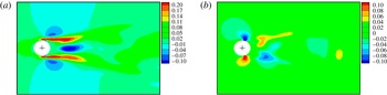
from (4.2). We plot the streamwise and the normal components of the control mode in figure 4. The key advantage of this method is that the flow perturbations in the control mode are not restricted to the local regions close to the actuators. Rather, the effect of the difference between the two average fields is also present in the wake. Appropriate application of the control input, using this function, can favourably alter the flow field over a wider part of the domain. In other words, the global aspect of this method makes it a better candidate for the construction of the control mode. In the present setting, we use
 $\unicode[STIX]{x1D652}^{mod}$
and compute first 12 POD modes to develop a 12-dimensional reduced-order model. The first four dominant streamwise and cross-flow velocity POD modes are plotted in figures 5 and 6 respectively.
Control mode at
 $\mathit{Re}=200$
: (a) streamwise and (b) cross-flow components.

The streamwise velocity modes: (a)
 ${\it\Phi}_{1}^{u}$
, (b)
 ${\it\Phi}_{2}^{u}$
, (c)
 ${\it\Phi}_{3}^{u}$
, (d)
 ${\it\Phi}_{4}^{u}$
.

The cross-flow velocity modes: (a)
 ${\it\Phi}_{1}^{v}$
, (b)
 ${\it\Phi}_{2}^{v}$
, (c)
 ${\it\Phi}_{3}^{v}$
, (d)
 ${\it\Phi}_{4}^{v}$
.

It is important to emphasize that the objective of this study is to compute the functional gains obtained from a simple feedback control and analyse these functions to suggest effective location of the sensors. These sensors may be used later to develop estimators to develop better controllers. The reduced-order model, developed in (4.5), is a 12-dimensional system of nonlinear ordinary differential equations (ODEs). If we can stabilize the system linearly, we can in fact stabilize the complete dynamics of the full system. According to the Hartman–Grobman theorem (Arnold Reference Arnold1988), (a) the fixed point, say
 $\boldsymbol{x}=\boldsymbol{x}_{0}$
, of the nonlinear system of the form
 $\dot{\boldsymbol{x}}=\boldsymbol{f}(\boldsymbol{x})$
is stable when the fixed point
 $\boldsymbol{x}^{\ast }=0$
of the linear system is asymptotically stable and (b) the fixed point,
 $\boldsymbol{x}=\boldsymbol{x}_{0}$
, of the nonlinear system of the above form is unstable when the fixed point
 $\boldsymbol{x}^{\ast }=0$
of the linear system is unstable.
We linearize the system about its mean component to reduce the model to a standard linear time invariant (LTI) control problem and obtain
 $$\begin{eqnarray}\underbrace{\left[\begin{array}{@{}c@{}}\dot{\boldsymbol{z}}^{r}\\ \dot{u}\end{array}\right]}_{\dot{\boldsymbol{x}}}=\underbrace{\left[\begin{array}{@{}cc@{}}\boldsymbol{A}_{2}^{r} & \boldsymbol{A}_{3}^{r}\\ \mathbf{0}^{\text{T}} & 0\end{array}\right]}_{\unicode[STIX]{x1D63C}}\underbrace{\left[\begin{array}{@{}c@{}}\boldsymbol{z}^{r}\\ u\end{array}\right]}_{\boldsymbol{x}}+\underbrace{\left[\begin{array}{@{}c@{}}\boldsymbol{B}^{r}\\ 1\end{array}\right]}_{\boldsymbol{B}}u_{c}.\end{eqnarray}$$
Equation (4.14) is an
 $M+1$
system of linear ODEs. Following Rediniotis et al. (Reference Rediniotis, Ko, Yue and Kurdila1999), we use
 $u_{c}=\dot{u}$
as the control command for finite-dimensional control, which is a convenient form for better understanding and is consistent with the control theory. Thus,
 $u_{c}=\dot{u}$
is a new control input to the system,
 $\mathbf{0}$
is a zero vector of size
 $M$
and
 $T$
denotes the transpose. Thus, we have reduced the model to a standard LTI control problem. The reduced-order model developed thus far is an open-loop (OL) control system where the control input is not a function of the states of the system. In other words, any change in the states does not alter the control input. One approach to alter the dynamics of the system is to change the poles (eigenvalues) of the state matrix
 $\unicode[STIX]{x1D63C}$
in the complex plane. This also allows us to design a feedback controller such that states decay to zero.
In the present framework, we choose
 $u_{c}$
as a linear function of the states of the system to obtain
 $$\begin{eqnarray}u_{c}=-\unicode[STIX]{x1D646}\left[\begin{array}{@{}c@{}}\boldsymbol{z}^{r}\\ u\end{array}\right],\end{eqnarray}$$
where
 $\unicode[STIX]{x1D646}$
is a
 $1\times (M+1)$
matrix with constant gains. Substitution of (4.15) into (4.14) yields a CL system of the form
 $$\begin{eqnarray}\left[\begin{array}{@{}c@{}}\dot{\boldsymbol{z}}^{r}\\ \dot{u}\end{array}\right]=\underbrace{\left(\left[\begin{array}{@{}cc@{}}\boldsymbol{A}_{2}^{r} & \boldsymbol{A}_{3}^{r}\\ \mathbf{0}^{\text{T}} & 0\end{array}\right]-\left[\begin{array}{@{}c@{}}\boldsymbol{B}^{r}\\ 1\end{array}\right]\unicode[STIX]{x1D646}\right)}_{\mathbb{A}_{\boldsymbol{c}}}\left[\begin{array}{@{}c@{}}\boldsymbol{z}^{r}\\ u\end{array}\right].\end{eqnarray}$$
As the purpose of the control law is to stabilize the system, it is desired to have the poles of the system in the left half of the complex plane. In other words, we would like the eigenvalues of
 $\mathbb{A}_{c}$
to have negative real parts. This will guarantee exponential stability of the system.
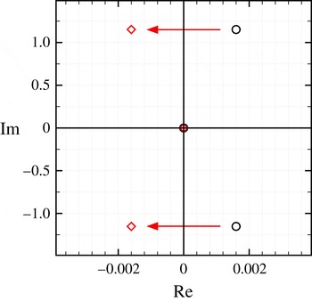
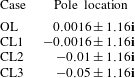
To analyse the system, we move the unstable complex conjugate pair of the OL system from the right half of the complex plane to the left half of the complex plane as shown in figure 7. We note that the imaginary part of the OL pole corresponds to the vortex shedding frequency and is kept the same for the new pole locations. The pole placement technique is one method to obtain a feedback gain that favourably alters the dynamics of the system. Other techniques include the LQR technique,
 $H^{2}$
control and
 $H^{\infty }$
control. We consider three CL systems with pole locations as listed in table 1. These systems are referred to as CL1, CL2, and CL3 respectively. The choice of pole location is often driven by design specifications, such as settling time, rise time, overshoot, etc.
Unstable poles moved to the left half of the complex plane.

Pole placement chart.

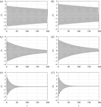
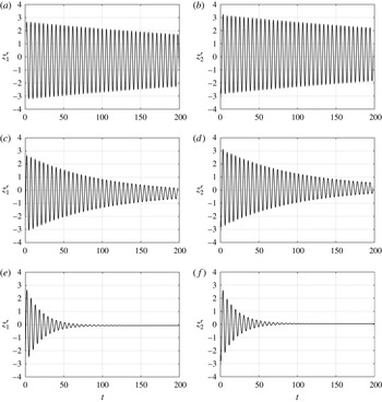
We compute appropriate gains for each CL system with the control calculated using the standard MATLAB function place which uses Ackerman’s algorithm (Ackermann Reference Ackermann1977). We then integrate the CL systems and observe their responses. In figure 8, we plot the response of the first two states
 $z_{1}^{r}$
and
 $z_{2}^{r}$
. Since the pole location is close to the imaginary axis, the system response of CL1 is slow and takes over 1000 time units to decay, with a settling time of approximately 2 %. On the other hand, the settling times of the CL2 and CL3 responses are approximately 300 and 120 time units respectively. The control input is linearly related to the states, thus
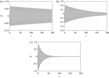
 $u_{c}$
also approaches zero in a similar fashion, as shown in figure 9. However, it is important to note that the movement of the poles is reflected in the control effort required to drive the states to zero. In other words, the maximum control input is close to 0.06, 0.21 and 0.8 for cases CL1, CL2 and CL3 respectively. Based on the control
 $\boldsymbol{u}(t)=-\mathscr{K}\boldsymbol{z}(t)+\mathscr{K}\boldsymbol{g}$
, the first component refers to
 $u_{c}$
, which makes the homogenized states go to zero, and the second component is the control input referring to constant suction input. For CL3, the constant suction is approximately 52 % of the free stream velocity (Akhtar & Nayfeh Reference Akhtar and Nayfeh2009).
Time history of
 $z_{1}^{r}$
(a,c,e) and
 $z_{2}^{r}$
(b,d,f) with control actuation: (a,b) CL1, (c,d) CL2 and (e,f) CL3.
Time history of
 $u_{c}$
with control actuation: (a) CL1, (b) CL2 and (c) CL3.

Using a similar model-based approach to control the vortex shedding past a cylinder, Akhtar et al. (Reference Akhtar, Naqvi, Borggaard and Burns2013) used an LQR technique to compute the appropriate gains and observed the system response. The objective was to reduce the fluctuating lift force to
 $$\begin{eqnarray}\min \int _{0}^{\infty }C_{L}^{2}(t)+Ru_{c}^{2}(t)\,\text{d}t,\end{eqnarray}$$
where
 $C_{L}$
is the lift coefficient,
 $R$
represents a control cost and the dynamics is described by the low-dimensional model derived above. The first two states correspond to the shedding frequency observed in the lift response. If the states
 $\boldsymbol{z}^{r}$
are stabilized, the lift coefficient is also reduced. Thus, the optimization problem was redefined as
 $$\begin{eqnarray}\min \int _{0}^{\infty }\boldsymbol{z}^{r^{\text{T}}}(t)\unicode[STIX]{x1D64C}\boldsymbol{z}^{r}(t)+Ru_{c}^{2}\,\text{d}t,\end{eqnarray}$$
where
 $\unicode[STIX]{x1D64C}_{M\times M}$
and
 $\unicode[STIX]{x1D64D}_{M_{c}\times M_{c}}$
are the state weighting matrix and the control effort weighting matrix respectively, with
 $M=12$
,
 $M_{c}=1$
,
 $\unicode[STIX]{x1D64C}=\unicode[STIX]{x1D644}$
and
 $\unicode[STIX]{x1D64D}=10$
. On feeding back the optimal gains, all of the states decay to zero. It is important to note that the gains obtained through LQR and pole placement are close, leading to a similar control response to that in CL3. Akhtar et al. (Reference Akhtar, Naqvi, Borggaard and Burns2013) also demonstrated that feeding back only the dominant state (
 $z_{1}^{r}$
) stabilizes the system, while feeding back only those states corresponding to higher modes fails to stabilize the system.
5. Functional gains
The feedback control gains given in (4.15) represent an approximation to the feedback operator associated with the PDE control system. The kernels of these operators, known as functional gains, provide an explicit representation of continuous linear feedback operators. In particular, we have
 $$\begin{eqnarray}u_{c}(t)=-\unicode[STIX]{x1D646}\left[\begin{array}{@{}c@{}}\boldsymbol{z}^{r}\\ u\end{array}\right]=-\unicode[STIX]{x1D646}_{z}\boldsymbol{z}^{r}(t)-K_{u}u(t),\end{eqnarray}$$
where
 $K_{u}\in \mathbb{R}$
and
 $\unicode[STIX]{x1D646}_{z}\boldsymbol{ : }\boldsymbol{H}\rightarrow \mathbb{R}$
is a bounded linear operator on the space of divergent free vector fields
 $\boldsymbol{H}$
. The Riesz representation theorem implies that there exists a divergent free vector field
 $\boldsymbol{h}(x)=(h^{u},h^{v})$
such that
 $$\begin{eqnarray}\displaystyle u_{c}(t) & = & \displaystyle -\unicode[STIX]{x1D646}_{z}\boldsymbol{z}^{r}(t)-K_{u}u(t)=-\int _{{\it\Omega}}\boldsymbol{h}(x)\boldsymbol{\cdot }\mathop{\sum }_{i=1}^{M}z_{i}^{r}(t){\it\Phi}_{i}(x)\,\text{d}{\it\Omega}-K_{u}u(t)\nonumber\\ \displaystyle & {\approx} & \displaystyle -\int _{{\it\Omega}}\boldsymbol{h}(x)\boldsymbol{\cdot }(\boldsymbol{v}(x,t)-\bar{\boldsymbol{v}}(x))\,\text{d}{\it\Omega}-K_{u}u(t).\end{eqnarray}$$
As mentioned before, the kernel
 $\boldsymbol{h}(x)$
is the functional gain associated with the fluid velocity.
Functional gains indicate how much information each state contributes to the control. One of the advantages of computing the functional gains is that they can be used to select good locations of control actuators/sensors in the flow domain. In particular, they indicate where the flow needs to be accurately sensed or estimated. If point measurements of
 $\boldsymbol{v}-\bar{\boldsymbol{v}}$
are sensed to compute the control, then the effective location of these points is related to a weighted quadrature problem.
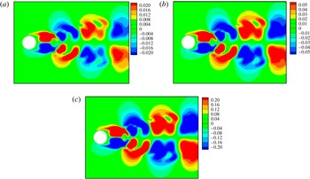
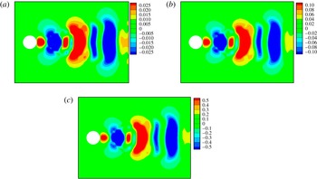
From (5.2), we compute the functional gains for the full-state feedback controls developed in table 1 using the first 12 POD modes. Figures 10 and 11 show the streamwise and cross-flow functional gains respectively, associated with the control laws CL1, CL2 and CL3. It is important to note that the contours for these gains have the same pattern but with different levels. Moreover, the support of the functional gains is concentrated in the wake of the cylinder, highlighting the region where the flow needs to be sensed or estimated most accurately.
Streamwise functional gain: (a) CL1, (b) CL2, (c) CL3.

Cross-flow functional gain: (a) CL1, (b) CL2, (c) CL3.

We note that the functional gain patterns are similar to the (negative) first streamwise velocity mode,
 ${\it\Phi}_{1}$
, leading to a positive correlation of
 $u_{c}$
with
 $z_{1}^{r}$
. To gain physical insight, we investigate the symmetries and distribution of the functional gains on the
 $(X,Y)$
axes. An obvious observation is the antisymmetric distribution of the streamwise functional gain (
 $h^{u}$
) with respect to the horizontal axis, i.e.
 $h^{u}(X,Y)=-h^{u}(X,-Y)$
. On the other hand, the cross-flow functional gain is symmetric with respect to the horizontal axis, i.e.
 $h^{v}(X,Y)=h^{v}(X,-Y)$
. The periodic control signal that we observe in practice is directly attributable to the pattern seen in figure 10(c) and the von Kármán vortex shedding. As the streamwise flow becomes symmetric, the contribution to the control signal vanishes as the positive and negative values of the (antisymmetric) functional gain weights cancel.
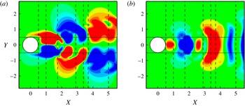
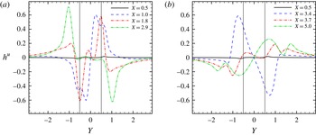
To elaborate more on the physical meaning of the functional gains, we consider case CL3 and plot the streamwise functional gain data in the wake. We choose seven stations in the wake and plot functional gains along vertical slices as shown in figure 12, corresponding to
 $X=0.5,1.0,1.8,2.9,3.4,3.7\text{ and }5.0$
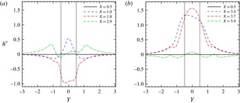
. The choice of these planes is motivated by the contour variation. We plot the streamwise (
 $h^{u}$
) and cross-flow (
 $h^{v}$
) functional gains in figures 13 and 14 respectively. For the purpose of clarity, we plot data from four planes in the subplots, with
 $X=0.5$
as a reference, while keeping the same axis for comparison. The solid horizontal lines at
 $Y=\pm 0.5$
in figures 13 and 14 indicate the diameter of the circular cylinder and highlight the maximum region of influence (ROI) in the wake.
Planes in the wake where functional gains are extracted. (a) Streamwise components. (b) Cross-flow components.

Streamwise functional gain extracted along the lines. (a) Locations closer in the wake; (b) locations far in the wake.

Cross-flow functional gain extracted along the lines. (a) Locations closer in the wake; (b) locations far in the wake.

In figure 13(a), the streamwise functional gain does not vary along the
 $X=0.5$
line and stays close to zero. As we move further into the wake at
 $X=1.0$
, we observe positive and negative peaks at
 $Y=0.2$
and
 $Y=-0.2$
respectively. Two peaks with lower magnitude at
 $Y=0.6$
and
 $Y=-0.6$
are also observed, thus increasing the range of values of the functional gain along this line. At
 $X=1.8$
, we observe sharp peaks at
 $Y=\pm 0.5$
with opposite magnitudes, while the centre has much lower magnitude. Further downstream in the wake at
 $X=2.9$
, distinctive but opposite peaks at
 $Y=\pm 1.0$
are observed and the gains remain close to zero within the ROI (
 $Y=\pm 0.5$
). In figure 13(b), at
 $X=3.4$
, we observe broader peaks around
 $Y=\pm 0.75$
, while further downstream, at
 $X=3.7$
and
 $X=5.0$
, the streamwise functional gains have lower magnitudes. It is also interesting to note that the streamwise functional gain has higher magnitudes within the ROI up to
 $X=1.8$
in the wake, whereas further downstream the absolute maximum occurs outside the ROI. Moreover, beyond
 $Y=\pm 1.3$
, the functional gain is less important, making it less desirable to sense the flow far away from the wake.
Similarly, we plot the cross-flow components of the functional gain (
 $h^{v}$
) in figure 14(a,b) along the same lines. The cross-flow components remain close to zero at
 $X=0.5$
and are included in both subplots for reference. In contrast to their streamwise counterparts, the cross-flow functional gains are symmetric with respect to the horizontal axis. At the
 $X=1.0$
plane, we observe a small peak about the centreline behind the cylinder. At
 $X=1.8$
, we observe a broad spectrum in the ROI which gradually decays to zero outside the region. The cross-flow functional gain is less significant in the plane
 $X=2.9$
and we observe peaks with much lower magnitudes at
 $Y=\pm 1.2$
. In figure 14(b), at
 $X=3.4$
and
 $X=3.7$
, we observe maximum amplitudes in this component of the functional gain within the ROI. On the other hand, at
 $X=5.0$
, the functional gain is close to zero.
6. Numerical experiments
Using distributed parameter control theory and the functional gains, we were able to identify regions in the flow domain where the sensors can be placed to effectively estimate the state of the system. Thus, by employing an ‘abstract’ idea from PDE control theory (the functional gain), one can gain insight into the practical issue of sensor location while maintaining reasonable computational cost.
6.1. Sensor placement
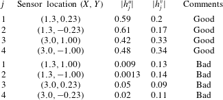
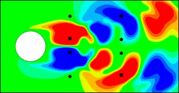
In order to validate our model and illustrate the idea, we consider the CL3 case to suggest the sensor locations in the wake of the cylinder. We simulate two scenarios. In each scenario, we use four locations to approximate the feedback gain given in (5.2). The choice of these locations is motivated by the magnitudes of the functional gain in the wake, in the
 $X=1.3$
and
 $X=3.0$
planes. In the first scenario, the four locations are chosen at the points where the functional gain is high (the good choice). On the contrary, we choose four locations with low functional gain magnitudes (the bad choice). The coordinates of these points along with the corresponding functional gains are provided in table 2. These locations are identified in figure 15 with good choice and bad choice scenarios represented by squares and circles respectively.
Sensor locations.

Functional gain approximated at four locations: good (square) and bad (circle) locations.

We approximate the feedback control input using a ‘quadrature’ as follows:
 $$\begin{eqnarray}\displaystyle u_{c}(t) & = & \displaystyle -\int _{{\it\Omega}}\boldsymbol{h}(x)\boldsymbol{\cdot }\mathop{\sum }_{i=1}^{12}z_{i}^{r}(t){\it\Phi}_{i}(x)\,\text{d}{\it\Omega}-K_{u}u(t)\nonumber\\ \displaystyle & {\approx} & \displaystyle -\mathop{\sum }_{j=1}^{4}\boldsymbol{h}_{j}\boldsymbol{\cdot }\mathop{\sum }_{i=1}^{12}z_{i}^{r}(t){\it\Phi}_{i}(x_{j})\,\text{d}A_{j}-K_{u}u(t),\end{eqnarray}$$
where
 $\boldsymbol{h}_{j}$
(in table 2) represents the mean value of
 $\boldsymbol{h}$
over the region
 $\text{d}A_{j}=\text{d}X\cdot \text{d}Y$
and
 $\text{d}X=\text{d}Y=0.2$
. We use the mean values of
 $\boldsymbol{h}_{j}$
over the region
 $\text{d}A_{j}$
to check the convergence of the functional gains. Using
 $M=12$
POD modes, the mean values of
 $\boldsymbol{h}_{j}$
converge to the magnitudes presented in table 2. Thus, we use these mean values of
 $\boldsymbol{h}_{j}$
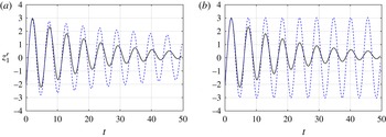
to compute the feedback control input. In figure 16, we simulate the reduced-order model with approximate gains computed from good and bad locations in the wake and compare it with a CL CFD simulation obtained from full-state feedback control.
Projection of a CL simulation (
 $z_{1}^{r}$
) with gains approximated at (a) good and (b) bad locations. It should be noted that the approximate gain (blue, dashed) is computed with only four sensors and the CL simulation gain (black, solid) is obtained with full-state feedback.

The approximation of the feedback gains provided by the good data set stabilizes the system, as shown in figure 16. Although the response is slow compared with the full-order feedback control, it is important to note that the gains were approximated from only four locations rather than using the complete domain. On the other hand, if the sensors are placed at bad locations, the feedback gain approximation is poor and fails to stabilize the CL system. Based on the current choice of sensor locations, figure 16(a,b) shows the two extremes of the system response to effective and ineffective controllers respectively. An obvious option to obtain a better response is to increase the number of sensors, but this is not feasible in most practical settings. Thus, it is important to choose the correct locations for the available sensors to measure or estimate the flow field.
6.2. Functional gains versus POD modes
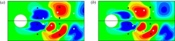
We emphasize that the functional gains provide an effective choice for sensor placement compared with other options, such as POD modes, wavemaker regions (Luchini, Giannetti & Pralits Reference Luchini, Giannetti and Pralits2008) or regions of absolute instability. To demonstrate the effectiveness of functional gains as the choice of sensor placement, we compare the streamwise POD modes with the streamwise functional gains, as shown in figure 17. It is important to note that the first two POD modes occur as a pair and contribute equally to capture over 95 % of the energy in the dynamical system. For direct comparison, we plot the first two streamwise POD modes in the upper half with the streamwise functional gain in the bottom half. Effective (good) and ineffective (bad) sensor locations, already determined based on the functional gains, are reproduced to compare their corresponding locations within the POD modes. A quick comparison reveals that the effective sensor locations can also be determined using the POD modes, and it may seem that placing sensors at large amplitudes of the POD modes would yield similar results to those obtained using the functional gains. However, this is not the case in general and may be misleading for effective sensor placement. To validate this statement, we choose sensor locations (white squares) where the magnitudes of the POD modes are relatively high while the corresponding functional gains are low. Arbitrary placement of a sensor at a location based on the POD mode can be ineffective, as seen from the results shown in figure 16(b). Conversely, there are locations (white circles) where there is no coherent structure present in the POD mode, but which correspond to a relatively high functional gain value and lead to a stable controlled system, as depicted in figure 16(a).
Comparison of first two streamwise POD modes (upper half) with the streamwise functional gain (bottom half). The functional gain is approximated at high (white square) and low (white circle) magnitudes of the POD modes. It should be noted that the black squares and black circles from figure 15 are plotted again for reference. (a) Plot of
 ${\it\Phi}_{1}^{u}$
versus
 $h^{u}$
; (b) plot of
 ${\it\Phi}_{2}^{u}$
versus
 $h^{u}$
.

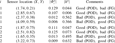
In table 3, we note the precise magnitudes of the POD modes and functional gains at the proposed sensor locations. For the first POD mode in figure 17(a), we identify two points,
 $(1.74,0.21)$
and
 $(2.85,0.67)$
, depicted as white squares, where the magnitude of the POD mode is of the order of 0.1 while the corresponding functional gains are one order of magnitude smaller. We term these locations as good points from the POD perspective but bad choices for control purposes since the functional gains are low. Similarly, sensor placement at the locations
 $(2.37,0.38)$
and
 $(4.09,0.59)$
(white circles) indicates bad choices from the POD mode perspective, but these locations have large functional gains, thus suggesting good sensor locations. Similar conclusions can be drawn from the analysis of the second POD mode. Based on figure 17, we emphasize again that there are locations in the POD modes where their high magnitudes overlap with high values of functional gains. However, our study above shows that solely identifying the locations where the dominant POD modes have large magnitudes cannot be used to determine effective sensor locations without additional considerations. The same concept can be used to explain the significance of functional gains over other techniques such as using the wavemaker region.
Comparison of sensor locations using POD modes and functional gains.

7. Conclusion
We used pole placement to design a feedback controller for flow past a cylinder where suction on the cylinder surface is used as a control mechanism. This linear controller is defined by an integral operator with kernel functions called functional gains. The functional gains are computed using POD-based reduced-order models. The reduced-order model has unstable poles that are consistent with the Strouhal frequency of vortex shedding past a cylinder at
 $\mathit{Re}=200$
. We developed three control laws based on pole placement to stabilize the system and studied their dynamics. In addition, we computed the functional gains that correspond to these feedback control laws and used the spatial information provided by these gains to investigate sensor locations. We showed that by locating the sensors where the functional gains have a large amplitude, we were able to preserve the stabilizing effect of the controller. On the other hand, placing the sensors in regions where the functional gains had small amplitude produced an unstable CL system. Thus, by computing the functional gains and using the spatial information contained in these gains we could determine where to place sensors in the wake region to ensure stability and performance. A comparison of placement strategies based on functional gains and POD modes also showed the significance of using functional gains for effective sensor placement.
The support of the functional gains suggests overlap with the wavemaker region identified for cylinder flows and needs to be explored further, see also Giannetti & Luchini (Reference Giannetti and Luchini2007), Luchini et al. (Reference Luchini, Giannetti and Pralits2008) and Marquet, Sipp & Jacquin (Reference Marquet, Sipp and Jacquin2008). This is natural, since the gain
 $-h(\cdot )$
would provide the feedback mechanism that would aid destabilization of the flow. Furthermore, the good locations found by choosing areas of large support can be robustly chosen so that small changes in the sensor locations will not dramatically affect the feedback signal of the controller. This is an important issue and, as shown in Chen & Rowley (Reference Chen and Rowley2011), several common choices for sensor location can be susceptible to this problem.
It should be observed that this analysis also provides valuable information concerning the construction of state estimators (filters). In particular, if one cannot physically place a sensor in the desired location in the wake, then one would design a filter to estimate the flow only in that region. Thus, this approach can produce reduced-order controllers without the need to reduce full-order compensators. This idea will be illustrated in a future paper where we will also compare these control laws with other robust control methods.
Acknowledgements
The first author would like thank COMSTECH-TWAS for their support under contract Research Grant Agreement (RGA) no. 11-208 RG/ENG/AS-C-UNESCO FR:3240262645. This research was also partially supported by the Air Force Office of Scientific Research under contract FA9550-12-1-0173 and by DOE contract DE-EE0004261 under subcontract no. 4345-VT-DOE-4261 from Pennsylvania State University. Numerical simulations were performed on the Virginia Tech Advanced Research Computing Center. The allocation grant and support provided by the staff are also gratefully acknowledged.
Appendix A. Numerical methodology
We briefly describe the numerical method used to generate the flow field data for the test problem in § 3.
We use a body-conformal ‘O’ type grid to simulate the flow over the cylinder and employ curvilinear coordinates in an Eulerian reference frame, as shown in figure 18. A non-staggered grid layout is employed to solve the transformed Navier–Stokes equations. The Cartesian velocity components (
 $v_{1},v_{2},v_{3}$
) and pressure (
 $p$
) are defined at the centre of the control volume in the computational space, and the volume fluxes (
 $V_{1},V_{2},V_{3}$
) are defined at the midpoints of its corresponding faces. All of the spatial derivatives are approximated with second-order-accurate central differences except for the convective terms, which are are discretized by using a variation of the QUICK algorithm (Leonard Reference Leonard1979).
The 2D layout of the ‘O’ grid in the (
 $r,{\it\theta}$
)-plane, showing the inflow and outflow directions.

A semi-implicit scheme is employed to advance the solution in time. The diagonal viscous terms are advanced implicitly using the second-order-accurate Crank–Nicolson method, whereas all of the other terms are advanced using the second-order-accurate Adams–Bashforth method. In the present formulation, we apply a fractional-step method (Kim & Moin Reference Kim and Moin1985; Orszag & Kells Reference Orszag and Kells1985; Street & Hussaini Reference Street and Hussaini1991; Zang, Street & Koseff Reference Zang, Street and Koseff1994; Chorin Reference Chorin1997) to advance the solution in time. The fractional-step method splits the momentum equation into (a) an advection–diffusion equation – a momentum equation solved without the pressure term – and (b) a pressure Poisson equation – constructed by implicit coupling between the continuity equation and the pressure in the momentum equation, thus satisfying mass conservation. The governing equations are solved using a methodology similar to that employed by Zang et al. (Reference Zang, Street and Koseff1994). However, the algorithm is extended to parallel computing platforms. To implement the algorithm on a distributed-memory message-passing parallel computer, we use domain decomposition technique such that each processor gets a ‘slice’ of the grid.
A schematic of the control actuator on the cylinder surface. (a) Location of the actuators; (b) velocity profiles on the actuators.

We employ no-slip and no-penetration boundary conditions on the cylinder surface. However, the boundary conditions can be modified to simulate other flow configurations, such as the case of a cylinder rotating along its axial direction. We can also enforce fixed or time-varying suction/blowing on the surface to perturb the flow field in the near vicinity of the cylinder for control purposes, as shown in figure 19(a). Time-periodic suction and blowing is a special case representing zero-net-mass-flux actuation, also known as a synthetic jet. The actuator is modelled by imposing a fixed or time-varying velocity normal to the cylinder surface. The defining parameters for the actuator are the peak velocity (
 $V_{j_{A}}$
), the operating frequency (
 $f_{j}$
), the location (
 ${\it\theta}_{j}$
) and the width (
 $S_{{\it\theta}}$
) of the jet orifice; that is,
 $$\begin{eqnarray}V_{j}=g({\it\theta}_{j})V_{j_{A}}\sin \left(2{\rm\pi}f_{j}\frac{U_{\infty }t}{d}+{\it\gamma}\right),\end{eqnarray}$$
where
 $j$
denotes ‘jet’ and not the index notation. In the actuator model,
 $g({\it\theta}_{j})$
defines the profile of the jet velocity as a function on
 $S_{{\it\theta}}$
, such as a top hat function, a sine function and a sine square function (see figure 19
b), and
 ${\it\gamma}$
is the phase.
In the current study, we use only suction on the cylinder surface for flow control, with a half-sine function profile spatially distributed on
 $S_{{\it\theta}}=10^{\circ }$
,
 $f_{j}=0$
,
 ${\it\gamma}={\rm\pi}/2$
. The numerical solver has been validated and verified, and the numerical results have been compared with other experimental and numerical studies (Akhtar Reference Akhtar2008; Akhtar et al.
Reference Akhtar, Marzouk and Nayfeh2009a
; Akhtar, Nayfeh & Ribbens Reference Akhtar, Nayfeh and Ribbens2009b
; Akhtar et al.
Reference Akhtar, Naqvi, Borggaard and Burns2013).
Appendix B. Reduced-order model
In the control function approach, we expand the velocity field as
 $$\begin{eqnarray}\boldsymbol{v}(x,t)\approx \bar{\boldsymbol{v}}(x)+\mathop{\sum }_{i=1}^{M}z_{i}^{r}(t){\it\Phi}_{i}(x)+\mathop{\sum }_{j=1}^{P}u_{j}(t){\it\Gamma}_{j}(x),\end{eqnarray}$$
where
 $P$
is the total number of control modes, the
 ${\it\Gamma}_{i}(x)$
are suitable divergence-free control functions that satisfy the inhomogeneous boundary condition due to fluidic actuators, and
 $\boldsymbol{u}(t)$
is the variable control input.
The reduced-order model developed here is more general and corresponds to
 $M$
POD modes and
 $P$
control modes. We note that (B 1) contains two time-dependent states,
 $z_{i}^{r}(t)$
and
 $u_{i}(t)$
. Therefore, we obtain two time derivative terms in the expansion as follows:
 $$\begin{eqnarray}\displaystyle \frac{\partial \boldsymbol{v}(x,t)}{\partial t} & = & \displaystyle \frac{\partial \bar{\boldsymbol{v}}(x)}{\partial t}+\frac{\partial }{\partial t}\left(\mathop{\sum }_{i=1}^{M}z_{i}^{r}(t){\it\Phi}_{i}(x)\right)+\frac{\partial }{\partial t}\left(\mathop{\sum }_{j=1}^{P}u_{j}(t){\it\Gamma}_{j}(x)\right)\nonumber\\ \displaystyle & = & \displaystyle \mathop{\sum }_{i=1}^{M}{\dot{z}}_{i}^{r}{\it\Phi}_{i}+\mathop{\sum }_{j=1}^{P}\dot{u}_{j}{\it\Gamma}_{j}.\end{eqnarray}$$
The convection term is more complex and generates both linear and nonlinear terms in the model. The quadratic terms obtained in the expansion are in
 $\boldsymbol{z}$
,
 $\boldsymbol{u}$
and their combinations; that is,
 $$\begin{eqnarray}\displaystyle \boldsymbol{v}\boldsymbol{\cdot }{\rm\nabla}^{h}\boldsymbol{v} & = & \displaystyle \left[\bar{\boldsymbol{v}}+\mathop{\sum }_{j=1}^{P}u_{j}{\it\Gamma}_{j}+\mathop{\sum }_{i=1}^{M}z_{i}^{r}{\it\Phi}_{i}\right]\boldsymbol{\cdot }{\rm\nabla}^{h}\left[\bar{\boldsymbol{v}}+\mathop{\sum }_{j=1}^{P}u_{j}{\it\Gamma}_{j}+\mathop{\sum }_{i=1}^{M}z_{i}^{r}{\it\Phi}_{i}\right]\nonumber\\ \displaystyle & = & \displaystyle \bar{\boldsymbol{v}}\boldsymbol{\cdot }{\rm\nabla}^{h}\bar{\boldsymbol{v}}+\bar{\boldsymbol{v}}\boldsymbol{\cdot }\mathop{\sum }_{j=1}^{P}u_{j}{\rm\nabla}^{h}{\it\Gamma}_{j}+\bar{\boldsymbol{v}}\boldsymbol{\cdot }\mathop{\sum }_{i=1}^{M}z_{i}^{r}{\rm\nabla}^{h}{\it\Phi}_{i}\nonumber\\ \displaystyle & & \displaystyle +\,\mathop{\sum }_{j=1}^{P}u_{j}{\it\Gamma}_{j}\boldsymbol{\cdot }{\rm\nabla}^{h}\bar{\boldsymbol{v}}+\mathop{\sum }_{j=1}^{P}u_{j}{\it\Gamma}_{j}\boldsymbol{\cdot }\mathop{\sum }_{j=1}^{P}u_{j}{\rm\nabla}^{h}{\it\Gamma}_{j}+\mathop{\sum }_{j=1}^{P}u_{j}{\it\Gamma}_{j}\boldsymbol{\cdot }\mathop{\sum }_{i=1}^{M}z_{i}^{r}{\rm\nabla}^{h}{\it\Phi}_{i}\nonumber\\ \displaystyle & & \displaystyle +\,\mathop{\sum }_{i=1}^{M}z_{i}^{r}{\it\Phi}_{i}\boldsymbol{\cdot }{\rm\nabla}^{h}\bar{\boldsymbol{v}}+\mathop{\sum }_{i=1}^{M}z_{i}^{r}{\it\Phi}_{i}\boldsymbol{\cdot }\mathop{\sum }_{j=1}^{P}u_{j}{\rm\nabla}^{h}{\it\Gamma}_{j}+\mathop{\sum }_{i=1}^{M}z_{i}^{r}{\it\Phi}_{i}\boldsymbol{\cdot }\mathop{\sum }_{i=1}^{M}z_{i}^{r}{\rm\nabla}^{h}{\it\Phi}_{i}.\end{eqnarray}$$
Rearranging the terms in (B 3) leads to
 $$\begin{eqnarray}\displaystyle \boldsymbol{v}\boldsymbol{\cdot }{\rm\nabla}^{h}\boldsymbol{v} & = & \displaystyle \bar{\boldsymbol{v}}\boldsymbol{\cdot }{\rm\nabla}^{h}\bar{\boldsymbol{v}}+\mathop{\sum }_{j=1}^{P}(\bar{\boldsymbol{v}}\boldsymbol{\cdot }{\rm\nabla}^{h}{\it\Gamma}_{j}+{\it\Gamma}_{j}\boldsymbol{\cdot }{\rm\nabla}^{h}\bar{\boldsymbol{v}})u_{j}+\mathop{\sum }_{i=1}^{M}(\bar{\boldsymbol{v}}\boldsymbol{\cdot }{\rm\nabla}^{h}{\it\Phi}_{i}+{\it\Phi}_{i}\boldsymbol{\cdot }{\rm\nabla}^{h}\bar{\boldsymbol{v}})z_{i}^{r}\nonumber\\ \displaystyle & & \displaystyle +\,\mathop{\sum }_{j=1}^{P}\mathop{\sum }_{k=1}^{P}({\it\Gamma}_{n}\boldsymbol{\cdot }{\rm\nabla}^{h}{\it\Gamma}_{k})u_{k}u_{j}+\mathop{\sum }_{k=1}^{M}\mathop{\sum }_{i=1}^{M}({\it\Phi}_{k}\boldsymbol{\cdot }{\rm\nabla}^{h}{\it\Phi}_{i})z_{k}^{r}z_{i}^{r}\nonumber\\ \displaystyle & & \displaystyle +\,\mathop{\sum }_{k=1}^{M}\mathop{\sum }_{j=1}^{P}({\it\Phi}_{k}\boldsymbol{\cdot }{\rm\nabla}^{h}{\it\Gamma}_{j}+{\it\Gamma}_{j}\boldsymbol{\cdot }{\rm\nabla}^{h}{\it\Phi}_{k})u_{j}z_{k}^{r}\end{eqnarray}$$
or in matrix form
 $$\begin{eqnarray}\displaystyle \boldsymbol{v}\boldsymbol{\cdot }\boldsymbol{{\rm\nabla}}\boldsymbol{v} & = & \displaystyle [\bar{\boldsymbol{v}}\boldsymbol{\cdot }{\rm\nabla}^{h}\bar{\boldsymbol{v}}]+[\bar{\boldsymbol{v}}\boldsymbol{\cdot }{\rm\nabla}^{h}{\it\Gamma}+{\it\Gamma}\boldsymbol{\cdot }{\rm\nabla}^{h}\bar{\boldsymbol{v}}]\boldsymbol{u}+[\bar{\boldsymbol{v}}\boldsymbol{\cdot }{\rm\nabla}^{h}{\it\Phi}+{\it\Phi}\boldsymbol{\cdot }{\rm\nabla}^{h}\bar{\boldsymbol{v}}]\boldsymbol{z}^{r}\nonumber\\ \displaystyle & & \displaystyle +\,\boldsymbol{u}^{\text{T}}[{\it\Gamma}\boldsymbol{\cdot }{\rm\nabla}^{h}{\it\Gamma}]\boldsymbol{u}+\boldsymbol{z}^{r^{\text{T}}}[{\it\Phi}\boldsymbol{\cdot }{\rm\nabla}^{h}{\it\Phi}]\boldsymbol{z}^{r}+\boldsymbol{u}^{\text{T}}[{\it\Gamma}\boldsymbol{\cdot }{\rm\nabla}^{h}{\it\Phi}+{\it\Phi}\boldsymbol{\cdot }{\rm\nabla}^{h}{\it\Gamma}]\boldsymbol{z}^{r},\end{eqnarray}$$
where the superscript T denotes the transpose of the vectors.
The diffusion term is also expanded as follows:
 $$\begin{eqnarray}\displaystyle {\it\Delta}^{h}\boldsymbol{v} & = & \displaystyle {\it\Delta}\left(\bar{\boldsymbol{v}}+\mathop{\sum }_{j=1}^{P}u_{j}{\it\Gamma}_{j}+\mathop{\sum }_{i=1}^{M}z_{i}^{r}{\it\Phi}_{i}\right)\nonumber\\ \displaystyle & = & \displaystyle {\it\Delta}^{h}\bar{\boldsymbol{v}}+\mathop{\sum }_{j=1}^{P}u_{j}{\it\Delta}^{h}{\it\Gamma}_{j}+\mathop{\sum }_{i=1}^{M}z_{i}^{r}{\it\Delta}^{h}{\it\Phi}_{i}.\end{eqnarray}$$
Combining equations,
 $$\begin{eqnarray}\dot{\boldsymbol{z}}^{r}=\boldsymbol{A}_{1}^{r}+\boldsymbol{A}_{2}^{r}\boldsymbol{z}^{r}+\boldsymbol{A}_{3}^{r}\boldsymbol{u}+\boldsymbol{F}_{1}^{r}(\boldsymbol{z}^{r})\boldsymbol{z}^{r}+\boldsymbol{F}_{2}^{r}(\boldsymbol{z}^{r})\boldsymbol{u}+\boldsymbol{F}_{3}^{r}(\boldsymbol{u})\boldsymbol{u}+\boldsymbol{B}^{r}\dot{\boldsymbol{u}},\end{eqnarray}$$
where the operators are represented by
 $$\begin{eqnarray}\displaystyle & \displaystyle [\boldsymbol{A}_{1}^{r}]_{k}=\frac{1}{\mathit{Re}}\langle {\it\Phi}_{k},{\it\Delta}^{h}\bar{\boldsymbol{v}}\rangle -\langle {\it\Phi}_{k},\bar{\boldsymbol{v}}\boldsymbol{\cdot }{\rm\nabla}^{h}\bar{\boldsymbol{v}}\rangle , & \displaystyle\end{eqnarray}$$
 $$\begin{eqnarray}\displaystyle & \displaystyle [\boldsymbol{A}_{2}^{r}]_{ki}=-\langle {\it\Phi}_{k},\bar{\boldsymbol{v}}\boldsymbol{\cdot }{\rm\nabla}^{h}{\it\Phi}_{i}\rangle -\langle {\it\Phi}_{k},{\it\Phi}_{i}\boldsymbol{\cdot }{\rm\nabla}^{h}\bar{\boldsymbol{v}}\rangle +\frac{1}{\mathit{Re}}\langle {\it\Phi}_{k},{\it\Delta}^{h}{\it\Phi}_{i}\rangle , & \displaystyle\end{eqnarray}$$
 $$\begin{eqnarray}\displaystyle & \displaystyle [\boldsymbol{A}_{3}^{r}]_{kp}=-\langle {\it\Phi}_{k},\bar{\boldsymbol{v}}\boldsymbol{\cdot }{\rm\nabla}^{h}{\it\Gamma}_{p}\rangle -\langle {\it\Phi}_{k},{\it\Gamma}_{p}\boldsymbol{\cdot }{\rm\nabla}^{h}\bar{\boldsymbol{v}}\rangle +\frac{1}{\mathit{Re}}\langle {\it\Phi}_{k},{\it\Delta}^{h}{\it\Gamma}_{p}\rangle , & \displaystyle\end{eqnarray}$$
 $$\begin{eqnarray}\displaystyle & [\boldsymbol{F}_{1}^{r}]_{kin}=-\langle {\it\Phi}_{k},{\it\Phi}_{i}\boldsymbol{\cdot }{\rm\nabla}^{h}{\it\Phi}_{n}\rangle , & \displaystyle\end{eqnarray}$$
 $$\begin{eqnarray}\displaystyle & [\boldsymbol{F}_{2}^{r}]_{kip}=-\langle {\it\Phi}_{k},{\it\Gamma}_{p}\boldsymbol{\cdot }{\rm\nabla}^{h}{\it\Phi}_{i}\rangle -\langle {\it\Phi}_{k},{\it\Phi}_{i}\boldsymbol{\cdot }{\rm\nabla}^{h}{\it\Gamma}_{p}\rangle , & \displaystyle\end{eqnarray}$$
 $$\begin{eqnarray}\displaystyle & [\boldsymbol{F}_{3}^{r}]_{kpq}=-\langle {\it\Phi}_{k},{\it\Gamma}_{p}\boldsymbol{\cdot }{\rm\nabla}^{h}{\it\Gamma}_{q}\rangle , & \displaystyle\end{eqnarray}$$
 $$\begin{eqnarray}\displaystyle & [\boldsymbol{B}^{r}]_{kp}=-\langle {\it\Phi}_{k},{\it\Gamma}_{p}\rangle , & \displaystyle\end{eqnarray}$$
 $i,k,n=1,2,\ldots ,M$
and
 $p,q=1,2,\ldots ,P$
.