1 Introduction
Viscoplastic, or, equivalently, yield-stress fluids form an important class of non-Newtonian materials in engineering and geophysics (Ancey Reference Ancey2007; Mitsoulis Reference Mitsoulis2007; Balmforth, Frigaard & Ovarlez Reference Balmforth, Frigaard and Ovarlez2014). When the yield stress is relatively strong, it has been suggested that flow can become ‘frustrated’ if the boundary conditions lock certain parts of the fluid into place whilst driving others into motion. This frustration is broken by the development of narrow viscoplastic boundary layers in the flow that provide lubrication and allow the rigid blocks to slide over one another (Chevalier et al. Reference Chevalier, Rodts, Chateau, Boujlel, Maillard and Coussot2013). Indeed, this dynamical behaviour was anticipated, nearly 70 years ago, by Oldroyd (Reference Oldroyd1947), who developed a theory for the boundary layers in a Bingham fluid.
Oldroyd’s key insight was to observe that inertia was not important in the thin boundary layers and, with a certain choice for their thickness, one could engineer a suitable balance of forces between viscous and plastic stresses. Unfortunately, continuing Oldroyd’s arguments to their conclusion leads to a complicated nonlinear boundary-layer equation that appears to be almost as challenging to solve as the original model equations. Consequently, there have been no subsequent attempts to derive general solutions to Oldroyd’s theory.
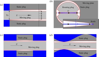
Despite the complexity of the boundary-layer equations, Oldroyd did derive two families of self-similar solutions that satisfied certain boundary conditions and applied them to two model problems: a jet-like intrusion and flow around a thin plate (see figure 1 a,b). For the former model problem, Oldroyd argued that two thin shear layers buffered the intrusion from the stagnant ambient medium, while for the latter, he suggested that the plate became coated by slender boundary layers. To our knowledge, the asymptotic reduction underlying Oldroyd’s boundary-layer theory has never been verified in these two problems, nor have his similarity solutions been shown to be relevant solutions of the boundary-layer equations. In fact, Oldroyd himself noted an inconsistency in the theory for the plate: his analysis was unable to impose all the boundary conditions at the edge of the boundary layer, leading Oldroyd to suggest that elastic deformations had to be included outside the boundary layer.
Sketches of the four model problems: (a) a jet-like intrusion from an inlet in a wall into a stagnant half-space, (b) flow past a thin plate moving in the direction of its length (with a finite plate shown in the main panel and a sketch of the semi-infinite knife overlaid), (c) channel flow through a sudden rectangular expansion and (d) flow down a wavy-walled conduit. Except for the semi-infinite knife, the sketches actually show the yield surfaces of solutions computed at high Bingham number (relatively large yield stress).

Aside from Oldroyd, the only other theoretical study of viscoplastic boundary layers was produced by Piau (Reference Piau2002), over half a century later, who reconsidered Oldroyd’s plate problem. Piau criticized the characteristic scalings that underlie Oldroyd’s analysis and proposed an alternative that suggests the boundary layer is actually thinner than that predicted by Oldroyd. In terms of a local Bingham number
 $B=\unicode[STIX]{x1D70F}_{Y}L/\unicode[STIX]{x1D707}\unicode[STIX]{x0394}U$
, Oldroyd predicted a boundary-layer scaling of
 $B^{-1/3}L$
, whereas Piau proposed the scaling
 $B^{-1/2}L$
. Here
 $L$
is the characteristic length of the boundary layer,
 $\unicode[STIX]{x0394}U$
is the typical velocity jump across it,
 $\unicode[STIX]{x1D70F}_{Y}$
is the yield stress and
 $\unicode[STIX]{x1D707}$
the plastic viscosity. Oldroyd’s scaling is based on balancing the viscous shear stress with pressure gradients and extensional plastic stresses. By contrast, Piau’s main force balance omits the extensional plastic stresses and can be achieved with any boundary-layer scaling in which the thickness is strictly less than Oldroyd’s; the precise reasoning behind his choice of the scaling
 $B^{-1/2}$
is not exposed. Moreover, after introducing the new scaling, Piau does not then provide a true asymptotic analysis of the boundary-layer equations, but retains some of the first-order corrections along with the leading-order terms in this system, and is then forced to propose some specific self-similar solutions rather than any general solution. This exercise is mysterious since a general solution can in fact be obtained by performing a strict asymptotic analysis and treating the two sets of terms at different orders in the expansion.
Despite these issues, Piau’s scaling is equivalent, at high Bingham number, to those that characterize exact solutions for plane-parallel flow of viscoplastic fluid (Bird, Dai & Yarusso Reference Bird, Dai and Yarusso1983), and to the viscoplastic version of Reynolds lubrication theory (e.g. Balmforth Reference Balmforth2017). Piau’s scaling was also observed in numerical simulations by Tokpavi, Magnin & Jay (Reference Tokpavi, Magnin and Jay2008) for the tangential boundary layer in two-dimensional flow around a disk. In all these examples, the boundary layer is bounded by a wall, which is the origin of the inconsistency in Oldroyd’s theory for flow around a plate.
Viscoplastic boundary layers have also been observed in a number of laboratory experiments, including the penetration of a plate into a stationary viscoplastic fluid (Boujlel et al. Reference Boujlel, Maillard, Lindner, Ovarlez, Chateau and Coussot2012) and pipe flow through a sudden expansion (Chevalier et al. Reference Chevalier, Rodts, Chateau, Boujlel, Maillard and Coussot2013). The former was motivated by the possibility of exploiting this scenario as a practical rheometer, and to provide an experimental viscoplastic analogue of both classical viscous boundary-layer theory and Oldroyd’s moving plate; the latter set the scene for Chevalier et al.’s appealing image of frustrated viscoplastic flow.
In the current paper, we revisit Oldroyd’s viscoplastic boundary-layer theory, and present a generalization of the theory that allows for the boundary layer to be curved and of finite length. We also begin from the Herschel–Bulkley constitutive model, rather than the Bingham law, to allow for the effects of shear thinning or thickening (although in all the examples we present, we retire to the Bingham case). We then apply this theory, and compare with the results of direct numerical simulations, to three model problems.
We first consider the jet-like intrusion (figure 1 a), and demonstrate that Oldroyd’s self-similar solutions apply. In the process, we uncover some additional features of the flow, including how the intrusion selects a new width for itself if the inlet through which it is pushed is too narrow. The means by which this width adjustment is achieved is by developing a finite region of perfectly plastic flow (Hill Reference Hill1950; Prager & Hodge Reference Prager and Hodge1951) near the inlet. We analyse the plastic region using the theory of sliplines, and the solution shows a number of common features with some classical plasticity problems related to the extrusion of metals from dies (Green Reference Green1955; Johnson Reference Johnson1956; Johnson, Sowerby & Venter Reference Johnson, Sowerby and Venter1982).
Second, we consider the flow of viscoplastic fluid past a slowly moving plate of finite length (figure 1
b) and, as in Piau’s critique, find that Oldroyd’s scalings do not apply to the boundary layer that sheathes the plate. Instead, we observe Piau’s scaling of
 $B^{-1/2}$
. However, the flow around the plate does not take the simple form anticipated by either Oldroyd or Piau, but instead takes a rather more complicated form that comprises both moving plugs and regions of perfectly plastic flow outside the boundary layer against the plate. Indeed, flow is induced over a roughly circular region with a diameter given by the length of the plate, rather than remaining localized near the plate. Importantly, this implies that one does not necessarily need to call on elastic deformation below the yield stress to account for motion further from the plate (cf. Boujlel et al.
Reference Boujlel, Maillard, Lindner, Ovarlez, Chateau and Coussot2012). Armed with the numerical solutions we provide an alternative boundary-layer theory that describes the leading-order features of the solutions.
Third, we explore flows down a channel with either a sudden expansion or wavy walls (figure 1
c,d). For these flows and at high yield stress, one expects viscoplastic boundary layers to detach from the walls to isolate a moving central plug from clogged topographic hollows, much as in Chevalier et al.’s frustrated pipe. We again provide numerical solutions to these problems and show the free shear layers are described by Oldroyd’s theory, but the presence of a wall adjacent to the boundary-layer effects a switch of scaling to Piau’s
 $B^{-1/2}$
scaling and the second type of boundary-layer theory.
2 Governing equations
For use in mapping out a general boundary-layer theory, we present the governing equations for a Herschel–Bulkley fluid in a curvilinear form. We then note the Cartesian version of these equations which are used in all our numerical computations (and for which we consider a Bingham fluid).
2.1 Curvilinear coordinates
Consider a curvilinear, arc-length-based coordinate system
 $(s,n)$
based on a curve threaded down an incompressible viscoplastic boundary layer;
 $s$
is the arc-length and
 $n$
is the normal coordinate. We define
 $\boldsymbol{u}=(u,v)$
as the velocity in these coordinates (i.e. with respect to the
 $(s,n)$
axes) and refer the deviatoric stress,
 $\unicode[STIX]{x1D70F}_{ij}$
, and deformation rate,
 $\dot{\unicode[STIX]{x1D6FE}}_{ij}$
, tensors to this system. With the neglect of inertia, conservation of mass and force balance can be expressed in the dimensionless form (e.g. Balmforth & Hewitt (Reference Balmforth and Hewitt2013), or derivable from relations given by Batchelor (Reference Batchelor1967)),
 $$\begin{eqnarray}\displaystyle & \displaystyle \frac{\unicode[STIX]{x2202}u}{\unicode[STIX]{x2202}s}+(1-\unicode[STIX]{x1D705}n)\frac{\unicode[STIX]{x2202}v}{\unicode[STIX]{x2202}n}-\unicode[STIX]{x1D705}v=0, & \displaystyle\end{eqnarray}$$
 $$\begin{eqnarray}\displaystyle & \displaystyle \frac{\unicode[STIX]{x2202}\unicode[STIX]{x1D70F}_{ss}}{\unicode[STIX]{x2202}s}+(1-\unicode[STIX]{x1D705}n)\frac{\unicode[STIX]{x2202}\unicode[STIX]{x1D70F}_{sn}}{\unicode[STIX]{x2202}n}-2\unicode[STIX]{x1D705}\unicode[STIX]{x1D70F}_{sn}=\frac{\unicode[STIX]{x2202}p}{\unicode[STIX]{x2202}s}, & \displaystyle\end{eqnarray}$$
 $$\begin{eqnarray}\displaystyle & \displaystyle \frac{\unicode[STIX]{x2202}\unicode[STIX]{x1D70F}_{sn}}{\unicode[STIX]{x2202}s}+(1-\unicode[STIX]{x1D705}n)\frac{\unicode[STIX]{x2202}\unicode[STIX]{x1D70F}_{nn}}{\unicode[STIX]{x2202}n}+\unicode[STIX]{x1D705}(\unicode[STIX]{x1D70F}_{ss}-\unicode[STIX]{x1D70F}_{nn})=\frac{\unicode[STIX]{x2202}p}{\unicode[STIX]{x2202}n}, & \displaystyle\end{eqnarray}$$
where
 $p$
is the pressure and
 $\unicode[STIX]{x1D705}$
denotes the curvature. The strain-rate tensor has components,
 $$\begin{eqnarray}\dot{\unicode[STIX]{x1D6FE}}_{ss}=\frac{2}{1-\unicode[STIX]{x1D705}n}\left(\frac{\unicode[STIX]{x2202}u}{\unicode[STIX]{x2202}s}-\unicode[STIX]{x1D705}v\right),\quad \dot{\unicode[STIX]{x1D6FE}}_{nn}=2\frac{\unicode[STIX]{x2202}v}{\unicode[STIX]{x2202}n},\quad \dot{\unicode[STIX]{x1D6FE}}_{sn}=\frac{1}{1-\unicode[STIX]{x1D705}n}\left(\frac{\unicode[STIX]{x2202}v}{\unicode[STIX]{x2202}s}+\unicode[STIX]{x1D705}u\right)+\frac{\unicode[STIX]{x2202}u}{\unicode[STIX]{x2202}n},\end{eqnarray}$$
which can be fed into the constitutive law:
 $$\begin{eqnarray}\left(\begin{array}{@{}c@{}}\unicode[STIX]{x1D70F}_{ss}\\ \unicode[STIX]{x1D70F}_{sn}\end{array}\right)=\left(\dot{\unicode[STIX]{x1D6FE}}^{N-1}+\frac{Bi}{\dot{\unicode[STIX]{x1D6FE}}}\right)\left(\begin{array}{@{}c@{}}\dot{\unicode[STIX]{x1D6FE}}_{ss}\\ \dot{\unicode[STIX]{x1D6FE}}_{sn}\end{array}\right)\quad \text{for}~\unicode[STIX]{x1D70F}\equiv \sqrt{\unicode[STIX]{x1D70F}_{ss}^{2}+\unicode[STIX]{x1D70F}_{sn}^{2}}>Bi,\end{eqnarray}$$
and
 $\dot{\unicode[STIX]{x1D6FE}}_{ij}=0$
otherwise, where
 $\dot{\unicode[STIX]{x1D6FE}}\equiv \sqrt{\dot{\unicode[STIX]{x1D6FE}}_{ss}^{2}+\dot{\unicode[STIX]{x1D6FE}}_{sn}^{2}}$
. To arrive at this scaled system, we have used a length scale
 ${\mathcal{L}}$
and characteristic speed
 ${\mathcal{U}}$
to remove the dimensions of length and velocity; the stresses and pressure are scaled by
 $\unicode[STIX]{x1D707}{\mathcal{U}}/{\mathcal{L}}$
, resulting in the global Bingham number,
 $$\begin{eqnarray}Bi=\frac{\unicode[STIX]{x1D70F}_{Y}{\mathcal{L}}}{\unicode[STIX]{x1D707}{\mathcal{U}}},\end{eqnarray}$$
where
 $\unicode[STIX]{x1D707}=K({\mathcal{U}}/{\mathcal{L}})^{N-1}$
is a characteristic viscosity,
 $K$
is the consistency,
 $N$
is the power-law index and
 $\unicode[STIX]{x1D70F}_{Y}$
is the yield stress. We choose
 ${\mathcal{L}}$
to be related to the overall size of the flow domain (which is finite in all computations); practically it provides a convenient measure of the length of the boundary layer. The speed scale
 ${\mathcal{U}}$
is imposed in all the problems we consider. (Note that
 $Bi$
is defined differently to the local Bingham number
 $B$
mentioned in the introduction, which involves the length and the velocity jump
 $\unicode[STIX]{x0394}U$
across the boundary layer.)
2.2 Cartesian form
For the simpler Cartesian coordinate system
 $(x,y)$
, the corresponding governing equations are
 $$\begin{eqnarray}u_{x}+v_{y}=0,\end{eqnarray}$$
 $$\begin{eqnarray}\frac{\unicode[STIX]{x2202}p}{\unicode[STIX]{x2202}x}=\frac{\unicode[STIX]{x2202}\unicode[STIX]{x1D70F}_{xx}}{\unicode[STIX]{x2202}x}+\frac{\unicode[STIX]{x2202}\unicode[STIX]{x1D70F}_{xy}}{\unicode[STIX]{x2202}y},\quad \frac{\unicode[STIX]{x2202}p}{\unicode[STIX]{x2202}y}=\frac{\unicode[STIX]{x2202}\unicode[STIX]{x1D70F}_{xy}}{\unicode[STIX]{x2202}x}-\frac{\unicode[STIX]{x2202}\unicode[STIX]{x1D70F}_{xx}}{\unicode[STIX]{x2202}y},\end{eqnarray}$$
 $$\begin{eqnarray}\left(\begin{array}{@{}c@{}}\unicode[STIX]{x1D70F}_{xx}\\ \unicode[STIX]{x1D70F}_{xy}\end{array}\right)=\left(\dot{\unicode[STIX]{x1D6FE}}^{N-1}+\frac{Bi}{\dot{\unicode[STIX]{x1D6FE}}}\right)\left(\begin{array}{@{}c@{}}2u_{x}\\ v_{x}+u_{y}\end{array}\right)\quad \text{for}~\unicode[STIX]{x1D70F}\equiv \sqrt{\unicode[STIX]{x1D70F}_{xx}^{2}+\unicode[STIX]{x1D70F}_{xy}^{2}}>Bi,\end{eqnarray}$$
and
 $u_{x}=u_{y}+v_{x}=0$
otherwise, where
 $\dot{\unicode[STIX]{x1D6FE}}=\sqrt{(u_{y}+v_{x})^{2}+4u_{x}^{2}}$
. Here, we have used subscripts of
 $x$
and
 $y$
to denote partial derivatives of the velocity components.
3 Boundary-layer theory
3.1 Oldroyd’s equation for a viscoplastic shear layer
Consider a shear layer of thickness
 $\unicode[STIX]{x1D716}=Bi^{-1/(N+2)}\ll 1$
. We rescale coordinates to resolve the narrow region:
 $$\begin{eqnarray}n=\unicode[STIX]{x1D716}\unicode[STIX]{x1D702},\quad \left[\begin{array}{@{}c@{}}u\\ v\end{array}\right]=\left[\begin{array}{@{}c@{}}U(s,\unicode[STIX]{x1D702})\\ \unicode[STIX]{x1D716}V(s,\unicode[STIX]{x1D702})\end{array}\right],\quad p=\frac{P(s,\unicode[STIX]{x1D702})}{\unicode[STIX]{x1D716}^{N+1}},\end{eqnarray}$$
 $$\begin{eqnarray}\unicode[STIX]{x1D70F}_{sn}=\frac{\unicode[STIX]{x1D70E}}{\unicode[STIX]{x1D716}^{N+2}}+\frac{\check{\unicode[STIX]{x1D70F}}_{sn}(s,\unicode[STIX]{x1D702})}{\unicode[STIX]{x1D716}^{N}},\quad \left[\begin{array}{@{}c@{}}\unicode[STIX]{x1D70F}_{ss}\\ \unicode[STIX]{x1D70F}_{nn}\end{array}\right]=\frac{1}{\unicode[STIX]{x1D716}^{N+1}}\left[\begin{array}{@{}c@{}}\check{\unicode[STIX]{x1D70F}}_{ss}(s,\unicode[STIX]{x1D702})\\ \check{\unicode[STIX]{x1D70F}}_{nn}(s,\unicode[STIX]{x1D702})\end{array}\right],\end{eqnarray}$$
where
 $\unicode[STIX]{x1D70E}=\text{sgn}(u_{n})$
. The rescaled conservation equations are, to leading order and assuming the curvature
 $\unicode[STIX]{x1D705}$
is
 $O(1)$
,
 $$\begin{eqnarray}U_{s}+V_{\unicode[STIX]{x1D702}}=0,\end{eqnarray}$$
 $$\begin{eqnarray}P_{s}=\frac{\unicode[STIX]{x2202}\check{\unicode[STIX]{x1D70F}}_{sn}}{\unicode[STIX]{x2202}\unicode[STIX]{x1D702}}+\frac{\unicode[STIX]{x2202}\check{\unicode[STIX]{x1D70F}}_{ss}}{\unicode[STIX]{x2202}s},\quad P_{\unicode[STIX]{x1D702}}=\frac{\unicode[STIX]{x2202}\check{\unicode[STIX]{x1D70F}}_{nn}}{\unicode[STIX]{x2202}\unicode[STIX]{x1D702}}\end{eqnarray}$$
(and again denoting partial derivatives by the subscripts
 $s$
and
 $\unicode[STIX]{x1D702}$
). The expansion of the constitutive law for yielded fluid gives
 $$\begin{eqnarray}\check{\unicode[STIX]{x1D70F}}_{sn}=|U_{\unicode[STIX]{x1D702}}|^{N-1}U_{\unicode[STIX]{x1D702}}-\frac{2\unicode[STIX]{x1D70E}U_{s}^{2}}{U_{\unicode[STIX]{x1D702}}^{2}},\quad \check{\unicode[STIX]{x1D70F}}_{ss}=-\check{\unicode[STIX]{x1D70F}}_{nn}=\frac{2\unicode[STIX]{x1D70E}U_{s}}{U_{\unicode[STIX]{x1D702}}}.\end{eqnarray}$$
Eliminating the pressure furnishes Oldroyd’s boundary-layer equation,
 $$\begin{eqnarray}\left(|U_{\unicode[STIX]{x1D702}}|^{N-1}U_{\unicode[STIX]{x1D702}}-\frac{2\unicode[STIX]{x1D70E}U_{s}^{2}}{U_{\unicode[STIX]{x1D702}}^{2}}\right)_{\unicode[STIX]{x1D702}}+4\unicode[STIX]{x1D70E}\left(\frac{U_{s}}{U_{\unicode[STIX]{x1D702}}}\right)_{s}=G(s),\end{eqnarray}$$
where
 $G(s)$
is an arbitrary function of
 $s$
generated by the
 $\unicode[STIX]{x1D702}$
-integral of the second relation in (3.4). Note that the scaling
 $\unicode[STIX]{x1D716}=Bi^{-1/(N+2)}$
for the boundary layer is designed to achieve the balance of terms in (3.6) and preceding equations.
For a shear layer sandwiched between two rigid plugs, the velocity outside the boundary layer is either in linear translation or uniform rotation. For the former, it is more convenient to use a Cartesian coordinate system for the geometry, with the
 $x$
-axis threaded down the boundary layer. For the latter, circular polar coordinates,
 $(r,\unicode[STIX]{x1D703})$
, are appropriate with
 $s\equiv R\unicode[STIX]{x1D703}$
and
 $n\equiv r-R$
, where
 $R$
denotes the radial location of the midline of the shear layer. For either case, the shear layer ends at the finite position,
 $\unicode[STIX]{x1D702}=\unicode[STIX]{x1D702}_{\pm }(s)$
, corresponding to the yield surfaces. There, the boundary conditions are
 $U(s,\unicode[STIX]{x1D702}_{\pm })=\text{constant}$
and
 $U_{\unicode[STIX]{x1D702}}(s,\unicode[STIX]{x1D702}_{\pm })=0$
(with
 $U_{s}/U_{\unicode[STIX]{x1D702}}$
finite).
Other kinds of shear layers are feasible, however, in which the shear layer matches to a perfectly plastic flow rather than a rigid plug. In this situation one expects that the shear layer follows a slipline (characteristic curve) of the stress field of the plastic solution, which is not necessarily either straight or circular. The boundary conditions now become the matches,
 $U(s,\unicode[STIX]{x1D702})\rightarrow u_{_{P}}(s)$
and
 $U_{\unicode[STIX]{x1D702}}\rightarrow 0$
, where
 $u_{_{P}}(s)$
is the plastic flow speed along the slipline, because the plastic flow spans an order-one region in
 $n$
with a solution free of the fine boundary-layer scale.
Note that, so far, we have not considered the mass conservation equation (3.3). The integral of this relation over the boundary layer implies that
 $$\begin{eqnarray}\frac{\unicode[STIX]{x2202}}{\unicode[STIX]{x2202}s}\int _{\unicode[STIX]{x1D702}_{-}}^{\unicode[STIX]{x1D702}_{+}}U(s,\unicode[STIX]{x1D702})\,\text{d}\unicode[STIX]{x1D702}=\left[\frac{\unicode[STIX]{x2202}\unicode[STIX]{x1D702}_{+}}{\unicode[STIX]{x2202}s}U(s,\unicode[STIX]{x1D702}_{+})-V(s,\unicode[STIX]{x1D702}_{+})\right]-\left[\frac{\unicode[STIX]{x2202}\unicode[STIX]{x1D702}_{-}}{\unicode[STIX]{x2202}s}U(s,\unicode[STIX]{x1D702}_{-})-V(s,\unicode[STIX]{x1D702}_{-})\right]\!;\end{eqnarray}$$
i.e. the divergence of the flux along the shear layer must balance the inflow or outflow through its borders.
For the self-similar solution outlined presently, for which the shear layer meets rigid plugs at
 $\unicode[STIX]{x1D702}=\unicode[STIX]{x1D702}_{\pm }$
, this relation is satisfied automatically by the symmetry of the boundary-layer profile, and conveys no additional information; the sole use of (3.3) is to determine the transverse velocity component
 $V(s,\unicode[STIX]{x1D702})$
once
 $U(s,\unicode[STIX]{x1D702})$
is known. However, if one side of the boundary layer aligns with a wall and this symmetry is broken, as in the plate problem considered in § 5, (3.7) imposes a non-trivial constraint that cannot be satisfied if
 $V(s,\unicode[STIX]{x1D702})$
is prescribed at a yield surface on the other side of the boundary layer. This inconsistency was noted by Oldroyd, who suggested that one could relax the boundary condition at the yield surface by including a modest elastic deformation over the adjoining plug region; we find instead that Oldroyd’s boundary-layer scaling is simply not relevant when the viscoplastic boundary layer is adjacent to a wall.
3.2 Self-similar solutions
The boundary-layer equations have a more general self-similar solution than that given by Oldroyd. We set
 $$\begin{eqnarray}U=U_{M}+\unicode[STIX]{x0394}U\,f(\unicode[STIX]{x1D701}),\quad \unicode[STIX]{x1D701}=-\unicode[STIX]{x1D70E}\frac{\unicode[STIX]{x1D702}-\unicode[STIX]{x1D702}_{_{M}}}{Y(s)},\end{eqnarray}$$
where
 $U\rightarrow U_{\pm }$
for
 $\unicode[STIX]{x1D702}\rightarrow \unicode[STIX]{x1D702}_{\pm }$
,
 $U_{M}=(U_{+}+U_{-})/2$
,
 $\unicode[STIX]{x0394}U=|U_{+}-U_{-}|$
,
 $\unicode[STIX]{x1D702}_{_{M}}=(\unicode[STIX]{x1D702}_{+}+\unicode[STIX]{x1D702}_{-})/2$
and
 $Y(s)$
is the half-thickness of the shear layer (
 $\unicode[STIX]{x1D70E}\equiv \text{sgn}(U_{+}-U_{-})$
). This rescaling symmetrizes the solution about the centre of the shear layer and orientates
 $\unicode[STIX]{x1D701}$
so that
 $U_{\unicode[STIX]{x1D701}}\leqslant 0$
. The boundary conditions then become
 $$\begin{eqnarray}f(\pm 1)=\mp {\textstyle \frac{1}{2}},\quad f_{\unicode[STIX]{x1D701}}(\pm 1)=0.\end{eqnarray}$$
When the shear layer is buffered by rigid plugs,
 $U_{\pm }$
are constant, the symmetry about the centreline implies
 $G=0$
, and (3.6) demands that
 $$\begin{eqnarray}(|\,f_{\unicode[STIX]{x1D701}}|^{N-1}f_{\unicode[STIX]{x1D701}})_{\unicode[STIX]{x1D701}}=\unicode[STIX]{x1D706}\unicode[STIX]{x1D701},\quad \frac{\text{d}^{2}Y}{\text{d}s^{2}}=-\frac{\unicode[STIX]{x1D706}(\unicode[STIX]{x0394}U)^{N}}{4Y^{N+1}},\end{eqnarray}$$
where
 $\unicode[STIX]{x1D706}$
is a separation constant. Hence, in view of the boundary conditions at
 $\unicode[STIX]{x1D701}=\pm 1$
,
 $$\begin{eqnarray}f=-\frac{1}{2}\text{sgn}(\unicode[STIX]{x1D701})\frac{B_{\unicode[STIX]{x1D701}^{2}}\left(\displaystyle \frac{1}{2},1+\displaystyle \frac{1}{N}\right)}{B\left(\displaystyle \frac{1}{2},1+\displaystyle \frac{1}{N}\right)},\quad \unicode[STIX]{x1D706}=2\left[\frac{N\unicode[STIX]{x1D6E4}\left(\displaystyle \frac{3}{2}+\displaystyle \frac{1}{N}\right)}{\sqrt{\unicode[STIX]{x03C0}}\unicode[STIX]{x1D6E4}\left(\displaystyle \frac{1}{N}\right)}\right]^{N},\end{eqnarray}$$
where
 $\unicode[STIX]{x1D6E4}(a)$
and
 $B(a,b)$
are the gamma and beta functions and
 $B_{x}(a,b)$
is the incomplete beta function. One then has to solve the problem in (3.10b
) for
 $Y$
. There are solutions with
 $Y=Y_{E}$
and
 $Y_{s}=0$
at the right-hand end of the boundary layer (giving
 $U_{s}=0$
) with
 $$\begin{eqnarray}\left(\frac{\text{d}Y}{\text{d}s}\right)^{2}=\frac{\unicode[STIX]{x1D706}}{2N}(\unicode[STIX]{x0394}U)^{N}(Y^{-N}-Y_{E}^{-N}).\end{eqnarray}$$
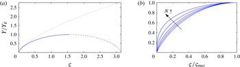
(a) Profile of the self-similar boundary-layer solution for
 $N=1$
(Bingham fluid) plotted against
 $\unicode[STIX]{x1D70D}=(s-s_{0})[\unicode[STIX]{x1D706}(\unicode[STIX]{x0394}U)^{N}/(2NY_{E}^{N+2})]^{1/2}$
, with
 $Y=0$
for
 $s=s_{0}$
and
 $(Y,Y^{\prime })=(Y_{E},0)$
at the right (solid); the solution can be continued to form a closed boundary layer as indicated by the dashed line. The dotted line shows
 $Y$
against
 $\sqrt{3\unicode[STIX]{x0394}U}(s-s_{0})/2$
, which is Oldroyd’s power-law solution (
 $N=1$
;
 $Y_{E}\gg 1$
). (b) Boundary-layer profiles for
 $N=0.1$
, 0.5, 1, 2 and 4, plotted against
 $\unicode[STIX]{x1D70D}/\unicode[STIX]{x1D70D}_{max}$
.

For the Bingham problem with
 $N=1$
, the boundary-layer solution reduces to
 $$\begin{eqnarray}f={\textstyle \frac{1}{4}}\unicode[STIX]{x1D701}(\unicode[STIX]{x1D701}^{2}-3),\quad \unicode[STIX]{x1D706}={\textstyle \frac{3}{2}},\end{eqnarray}$$
and
 $$\begin{eqnarray}Y_{E}^{3/2}\left[\tan ^{-1}\sqrt{\frac{\unicode[STIX]{x1D710}}{1-\unicode[STIX]{x1D710}}}-\sqrt{\unicode[STIX]{x1D710}(1-\unicode[STIX]{x1D710})}\right]_{\unicode[STIX]{x1D710}=Y_{0}/Y_{E}}^{Y/Y_{E}}=\frac{\sqrt{3\unicode[STIX]{x0394}U}}{2}(s-s_{0}),\end{eqnarray}$$
where
 $(s,Y)=(s_{0},Y_{0})$
denotes the start of the boundary layer. For
 $Y_{E}\rightarrow \infty$
, we recover Oldroyd’s power-law solution,
 $Y\propto s^{2/3}$
. Alternatively, if the boundary layer has a given length,
 $\ell$
, one obtains a relation between the thicknesses at inflow and exit:
 $$\begin{eqnarray}Y_{E}^{3/2}\left[\frac{1}{2}\unicode[STIX]{x03C0}-\tan ^{-1}\sqrt{\frac{Y_{0}}{Y_{E}-Y_{0}}}\right]-\sqrt{Y_{E}Y_{0}(Y_{E}-Y_{0})}=\frac{\sqrt{3\unicode[STIX]{x0394}U}}{2}\ell .\end{eqnarray}$$
In particular, if the boundary layer is closed at its initiation (
 $Y_{0}\rightarrow 0$
), then we find a maximum boundary-layer width, in terms of the original variable
 $n$
, of
 $$\begin{eqnarray}2Bi^{-1/3}Y_{E}=2Bi^{-1/3}\left(\sqrt{3\unicode[STIX]{x0394}U}\frac{\ell }{\unicode[STIX]{x03C0}}\right)^{2/3}\approx 1.345(\ell ^{2}\unicode[STIX]{x0394}U/Bi)^{1/3}.\end{eqnarray}$$
The boundary-layer profile predicted by (3.14) is plotted in figure 2(a). Note that the profile can be extended by its mirror image to furnish a solution that is closed at both its ends. Figure 2(b) compares boundary-layer profiles with different power-law indices
 $N$
, which all adopt a broadly similar shape. As mentioned above, for the remainder of this paper we restrict attention to the case of a Bingham fluid (
 $N=1$
).
4 Oldroyd’s jet-like intrusion
The first of Oldroyd’s model problems that we consider consists of a finger, or jet, of Bingham fluid pushed out of a vent in a wall to intrude into a half-space of stagnant fluid (figure 1 a). Oldroyd proposed that the borders between the finger and ambient would yield to form two thin viscoplastic shear layers with self-similar structure. We explore a slightly different version of the problem set in a finite domain, with symmetry conditions imposed to the right and on the top and bottom. We computed numerical solutions using an augmented Lagrangian scheme and a mixed finite-difference and spectral discretization, details of which are outlined in the Appendix.
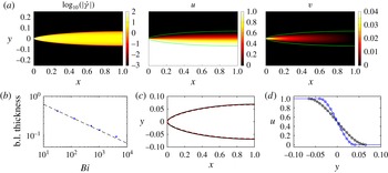
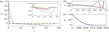
(a) Numerical solutions for a one-sided intrusion at
 $Bi=1024$
, with a symmetry line at
 $x=1$
, showing (from left to right)
 $\log _{10}(\dot{\unicode[STIX]{x1D6FE}})$
,
 $u$
and
 $v$
. The yield surface is shown as a green line. (b) The thickness of the shear layer at
 $x=1$
(dots), together with the asymptotic prediction (3.16) (dashed). (c) The yield surface (black) together with the prediction
 $Y/Bi^{1/3}$
(red, dashed) from the boundary-layer asymptotics. (d) Horizontal velocity profiles at
 $x=1$
(black) and
 $x=0.25$
(blue), together with the predicted profiles from the boundary-layer theory (circles).

4.1 A one-sided intrusion
When the inlet spans half of the
 $y$
-axis, a one-sided intrusion is thrust into the domain to form a single shear layer, furnishing the simplest possible setting for Oldroyd’s boundary-layer theory. More specifically, in the computations, we impose
 $u(0,y)=0$
for
 $y>0$
and
 $u(0,y)=1$
for
 $y<0$
, both with
 $v(0,y)=0$
.
A numerical solution is shown in figure 3 for
 $Bi=1024$
. As expected, a gradually widening shear layer develops at the edge of the intrusion with a distinctive shape characterized by its yield surfaces. Computations with different Bingham numbers establish that the thickness of the shear layer scales like
 $Bi^{-1/3}$
, as predicted by Oldroyd (figure 3
b). In (c,d), the yield surfaces and the profiles of horizontal velocity at two vertical sections are compared with the self-similar boundary-layer solution derived in § 3.2. In this case, the shear layer must shrink to the point
 $x=y=0$
at the edge of the inlet, implying that
 $Y(0)=Y_{0}=0$
, whilst the symmetry condition at
 $x=x_{e}=1$
demands that
 $Y_{x}=0$
.
4.2 Two-sided intrusions
For two-sided intrusions, we impose a unit influx over an inlet of finite width on the
 $y$
-axis, such that
 $u(0,y)=1/(2y_{I})$
for
 $-y_{I}<y<y_{I}$
and
 $u(0,y)=0$
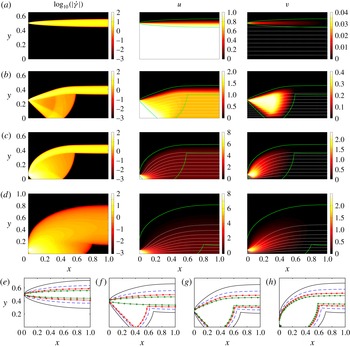
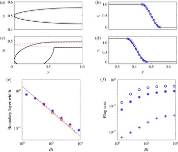
otherwise. Results from numerical simulations are shown in figure 4. For sufficiently large inlet widths
 $y_{I}$
(figure 4
a), the inflow takes the form of a plugged intrusion bordered by two viscoplastic boundary layers, exactly as suggested by Oldroyd. Each shear layer is essentially the same as that bordering the one-sided extrusion and again scales with
 $Bi^{-1/3}$
(see figure 5
e). Once more, the similarity solution for an initially closed boundary layer matches the numerical solution (see the shear layer shape and velocity profile in figure 5
a,b).
Intrusions for (a)
 $y_{I}=2^{-1}$
, (b)
 $y_{I}=2^{-2}$
and (c)
 $y_{I}=2^{-4}$
, all with
 $Bi=2048$
and showing only the upper half of the domain owing to symmetry at
 $y=0$
. Each row shows density plots of
 $\log _{10}(\dot{\unicode[STIX]{x1D6FE}})$
(left),
 $u(x,y)$
(centre) and
 $v(x,y)$
(right); the dotted (white) lines show a selection of streamlines and the solid (green) line shows the yield surfaces. (d) The same set of plots for
 $y_{I}=2^{-4}$
and
 $Bi=8$
; the flow is similar to the larger-
 $Bi$
solutions, but without distinct shear layers. (e–h) Yield surfaces for the same inlet widths as (a–c), together with the borderline case at
 $y_{I}=0.4$
, for
 $Bi=32$
(solid),
 $Bi=128$
(dashed),
 $Bi=512$
(▫) and
 $Bi=2048$
(○).

The (a,c) yield surfaces and (b,d) vertical profiles of horizontal velocity at
 $x=1$
, for intrusion with
 $Bi=2048$
and inlet half-widths of (a,b)
 $y_{I}=0.5$
and (c,d)
 $y_{I}=2^{-4}$
. Solid lines show the numerical solutions; dashed lines give the predicted boundary-layer shape
 $Y(y)$
, based on the measured velocity jump and centre line of the shear layers, and blue circles give the predicted velocity profiles from (3.13). (e) The thickness of the boundary layer at
 $x=1$
for
 $y_{I}=0.5$
(○) and
 $y_{I}=2^{-4}$
(*), together with the predictions from (3.16) using the measured velocity jumps (red solid line and blue dashed line, respectively), which asymptotically scale with
 $Bi^{-1/3}$
. (f) The axial length (○) and half-thickness (*) of the plugged intrusion and the position of the tip of the triangular plug at the inlet (
 $+$
), for
 $y_{I}=2^{-4}$
.

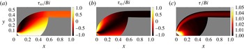
Further details of the stress field for the intrusion with
 $y_{I}=2^{-4}$
and
 $Bi=2048$
, which was shown in figure 4(c): density plots of (a)
 $\unicode[STIX]{x1D70F}_{xx}/Bi$
, (b)
 $\unicode[STIX]{x1D70F}_{xy}/Bi$
and (c)
 $\unicode[STIX]{x1D70F}/Bi$
. In view of the indeterminacy of the stress field over the rigid parts of the flow, the plugs are shaded grey.

However, when
 $y_{I}$
is decreased (figure 4
b,c), there is an abrupt change in the flow pattern: for sufficiently narrow inlets, the intrusion yields all the way down to the axis as it enters the domain and remains unplugged for some distance downstream. For
 $Bi\rightarrow \infty$
, this creates a finite region of perfectly plastic flow (cf. figures 4
g–h and 5
f), as illustrated in figure 6, which shows how the stress invariant is held very slightly above
 $Bi$
throughout. The plastic zones begin at the edges of the inlet, then widen and merge together to leave a small triangular tip to the incoming rigid jet. The plastic region splits apart further downstream at a yield surface that eventually closes off the plastic region. This closure leaves two horizontal viscoplastic boundary layers dividing a moving plug from the surrounding rigid ambient. Thus, if the inlet is too narrow, the extrusion plastically adjusts to reset its thickness close to some minimal value and recover Oldroyd’s flow pattern downstream. Note that the minimal half-thickness and the length of the horizontal section of the viscoplastic shear layer are both
 ${\sim}0.4$
for all the solutions with plastic zones at the inlet (when the horizontal length of the computational domain, and therefore the intrusion is unity).
The change in flow pattern occurs for
 $y_{I}$
less than 0.5. However, this threshold also depends slightly on Bingham number. Indeed, the solution with
 $y_{0}=0.4$
shown in figure 4 begins with a wide plastic region for lower
 $Bi$
, but then switches to two isolated shear layers for
 $Bi>512$
. For
 $Bi\gg 1$
, the mode change occurs for
 $y_{I}$
between 0.35 and 0.4, and seemingly closer to the latter than the former. We return to and clarify this point in § 4.3 below.
The shear layers at the edge of the plastic region that develop into the horizontal border of the plugged intrusion again follow Oldroyd’s
 $Bi^{-1/3}$
scaling throughout their length; see figure 5(e). Surprisingly, the self-similar solution nicely approximates the boundary-layer shape and velocity profile once the shear layer becomes horizontal (figure 5
c,d). This is not expected as, over the curved section where the shear layer borders the plastic region, the velocity jump is not constant and so the structure cannot be self-similar.
4.3 Plastic slipline theory
The perfectly plastic flow that arises in the overly narrow intrusions can be described using the slipline analysis of plasticity theory and is similar to some classical problems of the indentation and extrusion of metals (Hill Reference Hill1950; Green Reference Green1955; Johnson Reference Johnson1956; Johnson et al. Reference Johnson, Sowerby and Venter1982). The governing equations are those of stress equilibrium (2.8) with the deviatoric stresses satisfying the yield condition,
 $$\begin{eqnarray}\unicode[STIX]{x1D70F}^{2}=\unicode[STIX]{x1D70F}_{xx}^{2}+\unicode[STIX]{x1D70F}_{xy}^{2}=Bi^{2}.\end{eqnarray}$$
One can then deduce that the problem for the stress field is hyperbolic and the characteristics are the sliplines. With the definition,
 $$\begin{eqnarray}(\unicode[STIX]{x1D70F}_{xx},\unicode[STIX]{x1D70F}_{xy})=Bi(-\text{sin}\,2\unicode[STIX]{x1D717},\cos 2\unicode[STIX]{x1D717}),\end{eqnarray}$$
the
 $\unicode[STIX]{x1D6FC}$
and
 $\unicode[STIX]{x1D6FD}$
sliplines are given by
 $$\begin{eqnarray}\displaystyle \unicode[STIX]{x1D6FC}\text{-}\text{lines}:\quad \frac{\text{d}y}{\text{d}x}=\tan \unicode[STIX]{x1D717},\quad p+2Bi\unicode[STIX]{x1D717}=\text{const.}, & & \displaystyle\end{eqnarray}$$
 $$\begin{eqnarray}\displaystyle \unicode[STIX]{x1D6FD}\text{-}\text{lines}:\quad \frac{\text{d}y}{\text{d}x}=-\cot \unicode[STIX]{x1D717},\quad p-2Bi\unicode[STIX]{x1D717}=\text{const.}, & & \displaystyle\end{eqnarray}$$
and so
 $\unicode[STIX]{x1D717}$
is the anti-clockwise angular rotation of the
 $\unicode[STIX]{x1D6FC}$
-line from the
 $x$
axis.
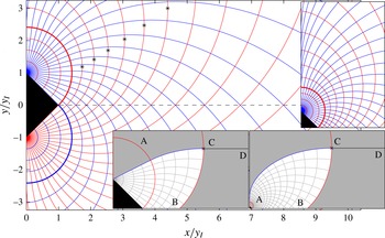
We describe the construction of the slipline field in the upper half-plane and with reference to figure 7. The construction begins using the circular arc
 $A$
of radius
 $y_{I}\sqrt{2}$
that is centred at the edge of the vent and intersects the tip of the rigid jet. Within this arc, the sliplines form a centred fan; we take the
 $\unicode[STIX]{x1D6FC}$
-line to be the straight radial spokes and the
 $\unicode[STIX]{x1D6FD}$
-characteristics to be the concentric circular arcs. Along the outermost
 $\unicode[STIX]{x1D6FD}$
-characteristic running along A, we have
 $p=p_{0}+2Bi\unicode[STIX]{x1D717}$
, where
 $p_{0}$
is an arbitrary background pressure level. The
 $\unicode[STIX]{x1D6FC}$
-lines passing through
 $A$
therefore have
 $p+2Bi\unicode[STIX]{x1D717}=p_{0}+4Bi\unicode[STIX]{x1D6E9}$
, where
 $\unicode[STIX]{x1D6E9}$
is the angle of these characteristics within the fan. Beyond
 $A$
, the
 $\unicode[STIX]{x1D6FC}$
-lines must curve down so that they intersect the
 $x$
-axis with
 $\unicode[STIX]{x1D717}=-\unicode[STIX]{x03C0}/4$
. Thence
 $p=p_{0}+4Bi\unicode[STIX]{x1D6E9}+(\unicode[STIX]{x03C0}Bi)/2$
at
 $y=0$
.
To build the slipline field beyond
 $A$
, we start with the lowest
 $\unicode[STIX]{x1D6FC}$
-line in the fan lying above the triangular face of the rigid jet. Using (4.3) and
 $\unicode[STIX]{x1D717}(x,0)=-\unicode[STIX]{x03C0}/4$
, this characteristic can be extended the short distance beyond
 $A$
down to its intersection with the
 $x$
-axis. The upgoing
 $\unicode[STIX]{x1D6FD}$
-line leaving that point can then be initiated and continued around the border of the fan using (4.3)–(4.4). Simultaneously, this extends all the
 $\unicode[STIX]{x1D6FC}$
-lines through
 $A$
out to the new
 $\unicode[STIX]{x1D6FD}$
-characteristic. The
 $\unicode[STIX]{x1D6FD}$
-characteristic terminates on the
 $y$
-axis above the fan with
 $\unicode[STIX]{x1D717}=\unicode[STIX]{x03C0}/2$
, where it launches a new
 $\unicode[STIX]{x1D6FC}$
-line that proceeds upwards and gradually bends away from the vertical. This procedure can then be repeated, extending the next lowest
 $\unicode[STIX]{x1D6FC}$
-line of the fan down to the
 $x$
-axis thereby beginning another
 $\unicode[STIX]{x1D6FD}$
-characteristic, and so forth; see figure 7.
Sliplines for the jet (
 $\unicode[STIX]{x1D6FC}$
-lines shown darker (blue),
 $\unicode[STIX]{x1D6FD}$
-lines lighter (red)). The stars show where
 $\unicode[STIX]{x1D6FD}$
-lines become vertical. The upper inset shows the sliplines over a larger region of the first quadrant, including more of the sliplines leaving the
 $y$
-axis above the fan. The lower insets show particular choices for the slipline and boundary layer that permit moving plugs bounded by
 $\text{BCD}$
.

To furnish a plastic region for the jet, we select one of the
 $\unicode[STIX]{x1D6FD}$
-characteristics with a base point B on the
 $x$
-axis. We then find the location C where this curve becomes vertical (cf. the selection of stars in figure 7). The section BC of this characteristic can be taken to be the left-hand border of the moving plug. At C, we begin the horizontal section of the viscoplastic shear layer (now assumed infinitesimally thin), and continue it to the right-hand border of the domain at D. Finally, the
 $\unicode[STIX]{x1D6FC}$
-line that passes through C forms the lower yield surface of the overlying stagnant fluid. Depending on the choice of the
 $\unicode[STIX]{x1D6FD}$
-line, the plastic region either extends up to an
 $\unicode[STIX]{x1D6FC}$
-line that leaves the fan, or incorporates the whole fan and is bounded by one of the
 $\unicode[STIX]{x1D6FC}$
-lines that departs tangentially from the
 $y$
-axis. The lower insets to figure 7 provide sample illustrations of the two situations. Although any of the
 $\unicode[STIX]{x1D6FD}$
-lines can be used for this construction, only one will satisfy the correct horizontal force balance condition on the moving plug, which depends on the domain length; i.e.
 $x_{D}$
.
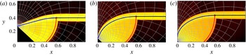
Slipline fields, with the plastic region bounded by the thicker sliplines and triangular face of the jet, superposed on density maps of
 $\log _{10}(\dot{\unicode[STIX]{x1D6FE}})$
with
 $Bi=2048$
from the numerical solutions, for inlet widths (a)
 $y_{I}=2^{-2}$
, (b)
 $y_{I}=2^{-4}$
and (c)
 $y_{I}=2^{-6}$
.

Instead of determining the correct
 $\unicode[STIX]{x1D6FD}$
-line for a given domain length, we turn the problem around and calculate the implied domain length for a given
 $\unicode[STIX]{x1D6FD}$
-line. In view of the symmetry condition imposed on the right border of the domain, there is no normal force along
 $x=x_{D}$
. The plug is therefore pushed forwards purely by the force from the plastic region along BC. This forward force is resisted by the drag from the viscoplastic shear layer CD, where the shear stress is
 $-Bi$
(cf. figure 6). Thence,
 $$\begin{eqnarray}-\int _{0}^{y_{C}}(p+Bi\tan \unicode[STIX]{x1D717})\,\text{d}y=Bi(x_{D}-x_{C}).\end{eqnarray}$$
An embarrassment with (4.5) is that the left-hand side contains the contribution
 $-p_{0}y_{C}$
of the arbitrary background pressure. However, in the viscoplastic shear layer, the pressure field should be constant to leading order (the spatially varying part of
 $p$
is
 $O(Bi^{-1/3})$
), and so the symmetry condition at
 $x=x_{D}$
demands that
 $p(x_{C},y_{C})\rightarrow 0$
, which fixes
 $p_{0}$
. With this choice, in figure 9(a) we plot
 $y_{C}/y_{I}$
and
 $(x_{D}-x_{C})/y_{I}$
against
 $x_{C}/y_{I}$
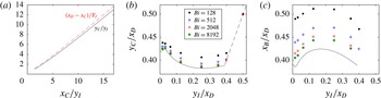
. Evidently, the jet half-width is approximately three-quarters of the length of the plastic region, whereas the length of the horizontal shear layer is comparable to the jet half-width. Both are consistent with the numerical results shown earlier. Given these quantities we may further formulate
 $y_{I}/x_{D}$
,
 $y_{C}/x_{D}$
and
 $x_{_{B}}/x_{D}$
, which corresponds to the scaling of the problem used in our numerical computations, and which are plotted in figure 9(b,c). For these scalings, the jet half-width is approximately 0.4 for a wide range of inlet sizes, and the slipline solutions dovetail satisfyingly with the limits suggested by the numerical solutions.
Plot of (a)
 $y_{C}/y_{I}$
and
 $(x_{D}-x_{C})/y_{I}$
against
 $x_{C}/y_{I}$
, then (b)
 $y_{C}/x_{D}$
and (c)
 $x_{B}/x_{D}$
, both against
 $y_{I}/x_{D}$
. The lines show the slipline solutions and the symbols, which correspond to different values of
 $Bi$
as indicated, show the numerical solutions. See figure 7 for the locations of A, B, C and D.

The computations in figure 9 contain a corner at
 $y_{I}/x_{D}\approx 0.032$
which corresponds to choosing the
 $\unicode[STIX]{x1D6FD}$
-line that becomes vertical where it intersects the
 $\unicode[STIX]{x1D6FC}$
-line that leaves the top of the fan with
 $\unicode[STIX]{x1D717}=\unicode[STIX]{x03C0}/2$
. That is, for
 $y_{I}/x_{D}>0.032$
the plastic region is bounded from above by an
 $\unicode[STIX]{x1D6FC}$
-line from the fan; for
 $y_{I}/x_{D}<0.032$
the plastic region extends above the fan and contains part of the
 $y$
-axis. The transition value is consistent with the numerical results, although there it is obscured by the viscous smoothing of the border of plastic region due to the finite Bingham number used in the computations.
The data also end for
 $y_{I}/x_{D}\approx 0.39$
; this limit corresponds to choosing the
 $\unicode[STIX]{x1D6FD}$
-line lying along the arc
 $A$
with
 $(x_{C},y_{C})=y_{I}(\sqrt{2},1)$
. Slipline solutions terminating in moving plugs cannot be found for wider inlets. This critical value is consistent with the switch in flow pattern observed numerically.
Finally, we note that we must take
 $y_{I}/x_{D}\rightarrow 0$
in order to approach the limit of an infinite domain, as in Oldroyd’s original vision of this problem. But figure 9 then implies that the plastic readjustment spans an infinitely wide region (
 $y_{C}/x_{D}$
and
 $x_{C}/x_{D}$
remain finite as
 $y_{I}/x_{D}\rightarrow 0$
). Thus, the intrusion must expand gradually outwards as a plastic readjustment and never lock into a bounded moving plug, implying Oldroyd’s prediction of isolated boundary layers only applies to a finite domain. Indeed, there is an intrinsic inconsistency with Oldroyd’s solution, because the boundary layers grow like
 $x^{2/3}$
and so will always collide in an infinite domain.
5 The finite plate
Oldroyd’s second model problem concerns a thin knife piercing a Bingham fluid. We consider a finite-length version of this problem, more suited to numerical computations, in which a plate of given length and zero thickness advances through a viscoplastic fluid in the same direction as its length (figure 1
b). For this problem, at high values of
 $Bi$
, one anticipates boundary layers to coat the plate and lubricate the motion through the fluid. This configuration has recently been the focus of an experimental study by Boujlel et al. (Reference Boujlel, Maillard, Lindner, Ovarlez, Chateau and Coussot2012), who claimed that one needs to supplement the viscoplastic boundary-layer solution with elastic-type deformation further from the plate to match the observed flow field, motivated perhaps by the contradiction arising in Oldroyd’s boundary-layer theory.
5.1 Numerical observations
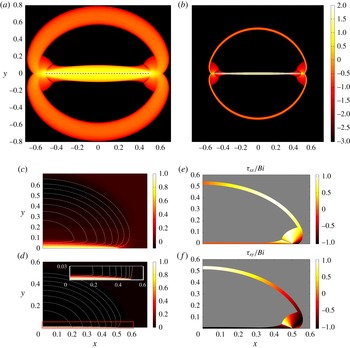
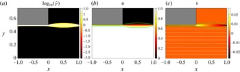
Numerical solutions to the problem are shown in figure 10. The plate does indeed advance through the fluid by creating slender viscoplastic boundary layers along its length, as found experimentally and suggested by Oldroyd. However, the fluid motion is not only confined to these boundary layers, as two other distinctive regions of flow also occur. First, and most noticeably, there is a circular viscoplastic boundary layer that lines the perimeter of the flowing region. This layer allows for the solid-body rotation of large rigid plugs above and below the plate (see figure 10 c,d). Second, fluid also yields at the front and back of the plate, over small but finite regions with perfectly plastic deformation. Both of these regions are identified by non-negligible levels of strain rate that are orders of magnitude lower than those experienced in the boundary layers against the plate (figure 10 a,b).
Flow around a plate of unit length for (a)
 $Bi=32$
and (b)
 $Bi=2048$
, showing density maps of
 $\log _{10}(\dot{\unicode[STIX]{x1D6FE}})$
. The dashed line locates the plate, which is moving from left to right with unit speed. (c,d) Density maps of the corresponding horizontal velocity component (displaying one quarter of the plane due to symmetry) for (c)
 $Bi=32$
and (d)
 $Bi=2048$
. Dashed white lines show a selection of streamlines. The inset in (d) shows a magnification of the boundary-layer flow against the plate, as indicated by the box of the main panel. (e,f) The normal and shear stress components, respectively, scaled by
 $Bi$
, for
 $Bi=2048$
.

Data as a function of
 $Bi$
. (a) Boundary-layer width at
 $x=0$
for the layer against the plate (
 $\ast$
) and for the circular shear layer (red
 $+$
). (b) Characteristic lengths of the plastic region: horizontal length in front of the tip of the plate
 $x_{a}-(1/2)$
(
 $\ast$
); maximum height
 $y_{b}$
of the stress discontinuity above the plate (blue
 $\circ$
); and maximum height
 $y_{p}$
of the plastic region (red
 $+$
). (c) Properties of the rotating plugs as defined in (5.11a,b
):
 $y_{c}$
(
 $\ast$
);
 $R-y_{c}-(1/2)$
(blue
 $\circ$
); and
 $Bi^{-1/2}\unicode[STIX]{x1D6FA}$
(red
 $+$
). The dashed lines show
 $Bi^{-1/2}$
and the (blue) circles in (a) plot the prediction in (5.10).

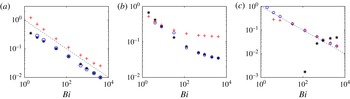
Critically, unlike the shear layers surrounding the intrusions, which scaled with
 $Bi^{-1/3}$
, the simulations show that the width of the boundary layer against the plate scales with
 $Bi^{-1/2}$
(figure 11
a), and the circular shear layer at the perimeter of the rotating plug also follows the same scaling. The latter observation can be explained by the fact that the velocity jump across the layer is not order one. Instead, we observe (and, in the following subsection, rationalize) that the rate of rigid rotation is
 $O(Bi^{-1/2})$
, while the radius of the rotating plug remains comparable to the order-one length of the plate. The velocity jump is thus
 $O(Bi^{-1/2})$
, and, given this scaling, the boundary-layer theory of § 3.2 predicts a shear-layer thickness of
 $O(Bi^{-1/2})$
(see (3.16)). In other words, the observed scaling of the circular shear layer is consistent with Oldroyd’s boundary-layer theory. We will deduce the basis for the
 $Bi^{-1/2}$
scaling of the boundary layers next to the plate in the next subsection.
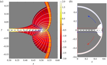
Over the regions of nearly plastic flow at the leading and trailing edges of the plate, we may diagnose the slipline field from the numerical solutions. As shown in figure 12(a), the slipline field contains a network emanating from an expansion fan that is located at the tip of the plate, together with a second network emerging from the viscoplastic boundary layer along the plate. The two networks are evidently incompatible and require a stress discontinuity to stitch them together (which is permissible in ideal plasticity if the tangential stress is discontinuous but the normal and shear stresses are continuous (Hill Reference Hill1950; Prager & Hodge Reference Prager and Hodge1951)).
Features of the flow near the front of the plate (black dashed) for
 $Bi=2048$
. (a) Sliplines (contours of
 $p\pm 2Bi\unicode[STIX]{x1D717}$
), as calculated from the numerical solutions, overlain on a density map of
 $\log _{10}\dot{\unicode[STIX]{x1D6FE}}$
. Grey regions indicate rigid plugs. (b) The centre of rotation (stars) and one quarter of the arc of rotation (dashed), for the counter-rotating plugs above and below the plate.

(a) Horizontal velocity profiles at
 $x=0$
for
 $Bi=32$
(black),
 $Bi=128$
(blue dashed),
 $Bi=512$
(red squares) and
 $Bi=2048$
(green circles). The inset shows the velocity across the rigid plug and outer circular boundary layer in more detail. (b,c) Details of the numerical solution for
 $Bi=2048$
: (b) the yield surface (black solid) and a contour of
 $\dot{\unicode[STIX]{x1D6FE}}=1$
(red dashed), which approximately demarcates the edge the viscoplastic boundary layer; and (c) the horizontal velocity profile at
 $x=0$
. Circles show the asymptotic predictions from (5.9), (5.4) and (5.10), using the measured values of
 $\unicode[STIX]{x1D6FA}$
,
 $R$
and
 $y_{c}$
.

Further details of the solutions, given in figures 11 and 13, are discussed in the following subsection. We note here that the centre of rotation of the rigid plugs enclosed by the circular shear layer is not quite at the centre of the plate, but slightly offset. The upper plug, for example, rotates about a point
 $y=-y_{c}$
on the
 $y$
-axis that is displaced a small distance below the plate (see figures 11
c and 12
b). In addition, that plug meets the plastic regions at the front and back edges of the plate along yield surfaces that correspond to particular sliplines.
5.2 Boundary-layer theory
For a plate moving to the right at unit speed, and in the laboratory frame, we rescale to introduce the boundary-layer coordinate
 $\unicode[STIX]{x1D702}=y/\unicode[STIX]{x1D716}$
and pressure
 $P(x,\unicode[STIX]{x1D702})=\unicode[STIX]{x1D716}^{2}p(x,y)$
, where
 $\unicode[STIX]{x1D716}$
is currently undetermined. We then have
 $$\begin{eqnarray}\frac{1}{\unicode[STIX]{x1D716}^{2}}P_{x}=\frac{1}{\unicode[STIX]{x1D716}}\frac{\unicode[STIX]{x2202}\unicode[STIX]{x1D70F}_{xy}}{\unicode[STIX]{x2202}\unicode[STIX]{x1D702}}+\frac{\unicode[STIX]{x2202}\unicode[STIX]{x1D70F}_{xx}}{\unicode[STIX]{x2202}x},\quad \frac{1}{\unicode[STIX]{x1D716}^{3}}P_{\unicode[STIX]{x1D702}}=\frac{\unicode[STIX]{x2202}\unicode[STIX]{x1D70F}_{xy}}{\unicode[STIX]{x2202}x}-\frac{1}{\unicode[STIX]{x1D716}}\frac{\unicode[STIX]{x2202}\unicode[STIX]{x1D70F}_{xx}}{\unicode[STIX]{x2202}\unicode[STIX]{x1D702}},\end{eqnarray}$$
where
 $$\begin{eqnarray}\unicode[STIX]{x1D70F}_{xy}\sim -Bi+\frac{1}{\unicode[STIX]{x1D716}}u_{\unicode[STIX]{x1D702}}+\cdots ,\quad \unicode[STIX]{x1D70F}_{xx}\sim -2\unicode[STIX]{x1D716}Bi\frac{u_{x}}{u_{\unicode[STIX]{x1D702}}}+\cdots\end{eqnarray}$$
(given
 $u_{\unicode[STIX]{x1D702}}<0$
). As long as
 $\unicode[STIX]{x1D716}^{3}Bi$
is small, we may neglect all but the leading-order terms to arrive at
 $$\begin{eqnarray}u_{\unicode[STIX]{x1D702}\unicode[STIX]{x1D702}}=P_{x},\quad P_{\unicode[STIX]{x1D702}}=0.\end{eqnarray}$$
Demanding that
 $u(x,0)=1$
and
 $(u,u_{\unicode[STIX]{x1D702}})\rightarrow 0$
for
 $\unicode[STIX]{x1D702}\rightarrow Y$
gives
 $$\begin{eqnarray}u=\left(1-\frac{\unicode[STIX]{x1D702}}{Y}\right)^{2},\quad P_{x}=\frac{2}{Y^{2}}.\end{eqnarray}$$
Mass conservation across the boundary layer implies
 $$\begin{eqnarray}v(x,y=\unicode[STIX]{x1D716}Y)=-\unicode[STIX]{x1D716}\frac{\unicode[STIX]{x2202}}{\unicode[STIX]{x2202}x}\int _{0}^{Y}u\,\text{d}\unicode[STIX]{x1D702}=-\frac{1}{3}\unicode[STIX]{x1D716}Y_{x}.\end{eqnarray}$$
Where the boundary layer meets the rigidly rotating cell above the plate, this transverse velocity must match the corresponding (anti-clockwise) rotation speed. The rotation rate must therefore be of the order of
 $\unicode[STIX]{x1D716}$
, so we set
 $\unicode[STIX]{x1D716}\unicode[STIX]{x1D6FA}(-y-y_{c},x)$
for the outer flow field, where the centre of rotation is at the point
 $(0,-y_{c})$
. Hence,
 $v(x,0)=\unicode[STIX]{x1D716}\unicode[STIX]{x1D6FA}x$
, and so
 $$\begin{eqnarray}Y=Y_{0}-{\textstyle \frac{3}{2}}\unicode[STIX]{x1D6FA}x^{2},\end{eqnarray}$$
where
 $Y(0)=Y_{0}$
is the central thickness. Evidently
 $$\begin{eqnarray}P_{x}=\frac{8}{(2Y_{0}-3\unicode[STIX]{x1D6FA}x^{2})^{2}}.\end{eqnarray}$$
Along any vertical cut through this part of the flowing region, we have the mass balance (ignoring the contribution of the circular boundary layer),
 $$\begin{eqnarray}\int _{0}^{Y}u\,\text{d}\unicode[STIX]{x1D702}\sim \unicode[STIX]{x1D6FA}\int _{0}^{y_{R}}(y+y_{c})\,\text{d}y,\end{eqnarray}$$
where
 $y_{R}=\sqrt{R^{2}-x^{2}}-y_{c}$
and
 $R$
is the radial extent of the rigid zone with respect to the rotation centre. That is,
 $$\begin{eqnarray}{\textstyle \frac{1}{3}}Y={\textstyle \frac{1}{2}}\unicode[STIX]{x1D6FA}(R^{2}-x^{2}-y_{c}^{2}).\end{eqnarray}$$
Thus
 $$\begin{eqnarray}Y_{0}={\textstyle \frac{3}{2}}\unicode[STIX]{x1D6FA}(R^{2}-y_{c}^{2}).\end{eqnarray}$$
Finally, we consider the magnitude of
 $\unicode[STIX]{x1D716}$
, which sets both the width of the boundary layer against the plate and the angular velocity of the rotating plug. The apparent constraint is that
 $\unicode[STIX]{x1D716}^{3}Bi\ll 1$
, which allows for any scaling smaller than
 $Bi^{-1/3}$
. In fact, the size of
 $\unicode[STIX]{x1D716}$
must be set by matching with the plastic region at the front and back of the knife. The relatively complicated slipline field over these regions demands that the pressure varies across them by
 $O(Bi)$
(because
 $p\pm 2Bi\unicode[STIX]{x1D717}$
, where
 $\unicode[STIX]{x1D717}$
is the angle of one of the sliplines, are the Riemann invariants). To match the pressure within the main viscoplastic boundary layer, we must therefore choose
 $\unicode[STIX]{x1D716}=Bi^{-1/2}$
, from the scalings introduced before (5.1). This matching of the pressure is the missing ingredient in Piau’s boundary-layer scaling argument.
At this stage, to fix the remaining
 $O(1)$
constants,
 $\unicode[STIX]{x1D6FA}$
,
 $R$
and
 $y_{c}$
, it seems necessary to work out the details of the plastic flow at the front and back edges of the plate. (The circular boundary layer must be matched to the plastic region, which requires its centreline to become tangential to the leading and trailing sliplines; force and torque balance must be imposed on the rotating plug.) We avoid this technical detail here, and settle for stating the fitted constants implied by the numerical solutions with
 $Bi\gg 1$
:
 $$\begin{eqnarray}\unicode[STIX]{x1D6FA}\approx 1,\quad (y_{c},R)\approx (0.06,0.56)\end{eqnarray}$$
(figure 11 c). The solutions also indicate that the plastic region has a spatial extent characterized by
 $$\begin{eqnarray}y_{p}\approx 0.14,\quad x_{a}-{\textstyle \frac{1}{2}}\approx y_{b}\approx 0.025,\end{eqnarray}$$
(figure 11
b), where
 $y_{p}$
is the maximum height of the plastic region,
 $x_{a}$
is the edge of the yield surface ahead of the plate (at
 $y=0$
), and
 $y_{b}$
is the height of the top of the stress discontinuity. Given these constants, the boundary-layer theory agrees well with data from numerical simulations (figure 13). Note that we find
 $R-y_{c}\sim (1/2)+O(Bi^{-1/2})$
(figure 11
c), indicating that the circular shear layer extends up to a height of exactly half the plate length; we have yet to find an explanation for this interesting numerical observation.
6 Channel flows of Bingham fluid
6.1 Flow through an expansion
For channel flow through a rectangular expansion, and in the limit of large yield stress, one expects the boundary layers along the walls of the main channel to become connected across the expansion by free shear layers. This type of flow was considered experimentally by Chevalier et al. (Reference Chevalier, Rodts, Chateau, Boujlel, Maillard and Coussot2013), who argued this to be a canonical viscoplastic analogue of the shear banding of plastic materials in ‘frustrated flows’ (Chevalier et al. considered pipe flow; we continue with the two-dimensional problem here).
We compute periodic solutions for flow with a unit flux along a channel with square-wave boundaries. More specifically, the channel is periodic on
 $-1<x<1$
, with boundaries located at
 $y=\pm 0.5$
for
 $-1<x<0$
and
 $y=\pm 1$
for
 $0<x<1$
(see the Appendix for more details of the numerical scheme). Figure 14 shows a sample solution for large
 $Bi$
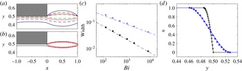
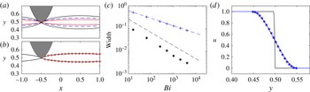
. As anticipated, free shear layers detach from the corners of the expansion to isolate the clogged-up well. At the corners, the shear layers thin sharply to merge with much narrower boundary layers against the channel walls. Computations from a suite of Bingham numbers (figure 15
c) indicate that the width of the free shear layers scales with
 $Bi^{-1/3}$
, as predicted by Oldroyd’s theory, but the width of the wall-bounded layers instead follows the
 $Bi^{-1/2}$
-scaling.
Periodic channel flow through a local expansion at
 $0<x<1$
with unit net flux down the channel and
 $Bi=2048$
. Density maps of (a)
 $\log _{10}\dot{\unicode[STIX]{x1D6FE}}$
; (b) the horizontal velocity; and (c) the vertical velocity. The dashed (white) lines show a selection of streamlines and the solid (green) line shows the yield surfaces.

Data for channel flow through an expansion. (a) Yield surfaces for
 $Bi=128$
(black),
 $Bi=512$
(blue dashed),
 $Bi=2048$
(red) and
 $Bi=8192$
(green dashed). (b) The yield surface (black) and the asymptotic prediction (○) from (3.13) for
 $Bi=2048$
. (c) The width of the free shear layer (blue pluses; measured at
 $x=0.5$
) and the wall-bounded layer (black stars; measured at
 $x=-0.5$
), together with dashed lines showing asymptotic predictions from (3.16), with scaling
 $Bi^{-1/3}$
, and (6.3), with scaling
 $Bi^{-1/2}$
, respectively. (d) Measured (lines) and predicted (symbols) profiles of the horizontal velocity
 $u(y)$
across the wall-bounded (black circles) and free (blue stars) shear layers.

Because the wall layers are so much narrower that the shear layer, that layer effectively closes at its ends. Thus, for the free shear layer, the maximum thickness of the boundary layer (which occurs at
 $x=1/2$
) is predicted from (3.16) to be
 $0.847Bi^{-1/3}$
(using
 $\ell =1/2$
). This prediction agrees satisfyingly with the numerical results, as shown in figure 15(c). Furthermore, the boundary-layer shape and velocity profile across the layer are also comfortably reproduced by (3.13) and (3.14) with
 $Y_{0}\rightarrow 0$
(figure 15
b,d).
For the wall layers, the theory in § 5.2 instead applies, although the change in the velocity conditions on the walls implies that
 $$\begin{eqnarray}u=1-\left(1-\frac{\unicode[STIX]{x1D702}}{Y}\right)^{2},\quad P_{x}=\frac{2}{Y^{2}},\end{eqnarray}$$
rather than (5.4), where
 $\unicode[STIX]{x1D702}\equiv \unicode[STIX]{x1D716}^{-1}((1/2)-y)$
, and again
 $\unicode[STIX]{x1D716}\ll Bi^{-1/3}$
is currently undetermined. As there is no flow into these boundary layers from the plug, the mass flux over the boundary layer must be constant, implying
 $Y_{x}=0$
. Thus, the boundary layer has uniform thickness
 $\unicode[STIX]{x1D716}Y$
and over the constricted part of the channel there must be a pressure drop of
 $$\begin{eqnarray}\unicode[STIX]{x0394}p=\frac{\unicode[STIX]{x0394}P}{\unicode[STIX]{x1D716}^{2}}=\frac{2d}{(\unicode[STIX]{x1D716}Y)^{2}},\end{eqnarray}$$
where
 $d=1$
is the length of the wall-bounded layer. Over the shear layer, however, the equivalent pressure drop is much less (of order
 $Bi^{2/3}$
). In other words, the full pressure drop across the entire channel is felt mostly over the constricted section. In view of the periodic boundary conditions imposed at
 $x=\pm 1$
, force balance on (half of) the moving plug demands that the force due to the pressure drop on the vertical sides matches the drag from combined boundary layers, where the shear stress is
 $Bi$
. Thus,
 $$\begin{eqnarray}{\textstyle \frac{1}{2}}\unicode[STIX]{x0394}p=2Bi\quad \text{or}\quad \unicode[STIX]{x1D716}Y=(2Bi)^{-1/2},\end{eqnarray}$$
and so the boundary-layer thickness is
 $O(Bi^{-1/2})$
. Note that this boundary layer is thinner by a factor of
 $\sqrt{2}$
than the corresponding boundary layer for flow down a uniform channel, entirely because the pressure drop is restricted to the constricted section. The prediction in (6.3), together with the velocity profile (6.1), again match nicely with the numerical computations (figure 15
c,d).
We also note that the shear layer and the wall layer are connected together across a relatively narrow matching region. Here the thickness of the shear layer decreases towards zero, implying a diverging pressure gradient. Both features allow the shear layer solution to be matched to that for the wall layer. The match also results in a small shift in the vertical position of the shear layer from the corner of the expansion, which we have measured and included in the asymptotic predictions in figure 15(b,d).
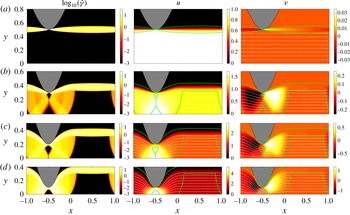
Solutions for periodic flow down a channel with boundaries located at
 $y=\pm (1+a\sin (\unicode[STIX]{x03C0}x))$
, for different amplitudes
 $a$
and
 $Bi=2048$
(only a part of the domain is shown). Density plots of
 $\log (\dot{\unicode[STIX]{x1D6FE}})$
(left),
 $u$
(centre) and
 $v$
(right), for amplitudes (a)
 $a=0.5$
, (b)
 $a=0.7$
, (c)
 $a=0.8$
and (d)
 $a=0.9$
. Streamlines (white dashed) and yield surfaces (green solid) are also shown in the plots of the velocity components.

6.2 Flow down a wavy-walled conduit
For flow down a wavy-walled channel, we computed solutions imposing unit flux along a conduit with sinusoidal width
 $y=\pm (1+a\sin \unicode[STIX]{x03C0}x)$
and periodic conditions at
 $x=\pm 1$
(further details again given in the Appendix). Results from a suite of computations are shown in figure 16. Provided the channel is not too constricted, shear layers develop that detach from the wavy wall where the conduit is thinnest, isolating plugged fluid in the wells of the topography (figure 16
a). If, however, the amplitude
 $a$
of the wavy wall is large enough to sufficiently constrict the channel, the flow pattern changes to include finite regions of plastic deformation. Sample flow patterns are displayed in figure 16(b–d), and give a sense of the plug phenomenology as the amplitude
 $a$
is varied. We have not attempted to explore these features in any detail, or to delve further into the wavy-wall solutions as a whole, in view of the previous study by Roustaei, Gosselin & Frigaard (Reference Roustaei, Gosselin and Frigaard2014) and forthcoming work by the same group.
Data from computations with amplitude
 $a=0.5$
. (a) Yield surfaces for
 $Bi=512$
(black),
 $Bi=2048$
(blue dashed) and
 $Bi=8192$
(red). (b) The yield surface (black) and the asymptotic prediction (○) from (3.13) for
 $Bi=2048$
. (c) The width of the free shear layer (blue pluses; measured at
 $x=0.5$
) and of the wall-bounded layer (black stars; measured at
 $x=-0.5$
), together with the asymptotic prediction (blue dashed line) from (3.16), with scaling
 $Bi^{-1/3}$
, and the predicted scaling for the wall layer of
 $Bi^{-7/12}$
(black dashed line). (d) Profiles of the horizontal velocity
 $u(y)$
at
 $x=-0.5$
(black) and
 $x=0.5$
(blue), together with the asymptotic prediction for the free shear layer (blue stars).

Instead, we briefly discuss the solutions for unconstricted channels, such as in figure 16(a), which can be directly compared with boundary-layer theory. Results from a suite of computations, shown in figure 17, indicate that the width of the shear layer again follows the
 $Bi^{-1/3}$
-scaling (figure 17
c), and both its width and velocity profile can be reproduced by the self-similar solution of § 3.2 (figure 17
b–d). The solutions are more complicated than for the rectangular expansions discussed in the previous section because the boundary layer that forms where the shear layer meets the wall (near
 $x=-0.5$
) is localized in both spatial directions. The length of the wall layer must be set by the topographic variation: we expect the layer to end where the topography, which is locally quadratic, widens to a width of order
 $Bi^{-1/3}$
, to match with the free shear layer. Thus the layer should have length
 $d\sim Bi^{-1/6}$
, which can be input directly into (6.2) to give an expected width
 $(\unicode[STIX]{x1D716}Y)\sim Bi^{-7/12}$
. The numerical results appear to support this scaling, as shown in figure 17(c).
7 Concluding remarks
Our goal in this article has been to shed light on the structure of the boundary layers that appear when yield stresses dominate a viscoplastic flow. Almost 70 years ago, Oldroyd argued for the existence of such narrow regions and presented an asymptotic theory to describe them. That theory is relatively complicated and the only solutions to date that we are aware of are some, again due to Oldroyd, that take a self-similar form. However, the characteristic scalings of Oldroyd’s theory have failed to be observed in some specific situations. Instead, scalings from a revision of the boundary-layer theory by Piau have been observed, calling into question the validity of Oldroyd’s theory.
Using a combination of numerical computations and a generalization of Oldroyd’s theory, we have demonstrated that certain viscoplastic boundary layers are indeed described by Oldroyd’s theory. In all these cases the boundary layers take the form of free viscoplastic shear layers lying between either rigid plugs or regions of perfectly plastic flow. The boundary layers, which are described by a balance between the pressure gradients, viscous shear stresses and leading-order plastic stresses, have a characteristic aspect ratio of the order of
 $B^{-1/3}$
for a Bingham fluid (or
 $B^{-1/(N+2)}$
for a Herschel–Bulkley fluid with power-law index
 $N$
).
We have, however, also found that Oldroyd’s theory does not apply to boundary layers that lie against a wall. The reason for this is related to the inability of the formulation to satisfy the correct transverse velocity conditions at both the wall and the other border of the layer: the boundary-layer solution is overconstrained by the requirement of mass conservation in this case. Oldroyd himself noted this problem with his theory and suggested that elastic stresses in the surrounding region might cure the problem; here, we instead interpret the problem simply to be that the characteristic scalings underlying Oldroyd’s analysis do not apply. Instead, one requires a different boundary-layer theory, in which the layer is thinner and the pressure gradient along it is balanced by viscous shear stresses alone, to leading order, as in the viscoplastic generalization of Reynolds’ lubrication theory. For Bingham fluid, this balance is consistent with Piau’s layer of aspect ratio
 $B^{-1/2}$
(or
 $B^{-1/(1+N)}$
for the Herschel–Bulkley law), although it equally applies to any layer that is asymptotically thinner than
 $B^{-1/3}$
, with the precise exponent for a given situation being set by the external pressure gradient.
Acknowledgement
The authors thank the Banff International Research Station for hosting the Focussed Research Group on Geophysical Viscoplastic Flows (November 2015) that initiated this research.
Appendix. Numerical scheme
To compute numerical solutions of the various problems considered in this paper, the governing Stokes equations (2.8)–(2.9) were solved using an augmented-Lagrangian scheme. This approach involves the iterative solution of a linear Stokes equation together with a set of nonlinear algebraic equations, which allows for accurate, if fairly slow, convergence and avoids the need for regularization of the nonlinear viscoplastic rheology. Both the method and its application to the study of viscoplastic fluids have been widely discussed in previous literature (e.g. Vinay, Wachs & Agassant Reference Vinay, Wachs and Agassant2005; Dean, Glowinski & Guidoboni Reference Dean, Glowinski and Guidoboni2007), to which the interested reader is referred.
The linear Stokes equation was written as a biharmonic equation for the streamfunction, and solved at each step of the iteration procedure over the domain
 $0<x<x_{u}$
and
 $0<y<y_{u}$
using a Fourier transform in one direction and second-order finite differences in the other. The details of the method, together with the choice of
 $x_{u}$
and
 $y_{u}$
, vary depending on the specific problem being solved. For jets, we chose
 $x_{u}=1$
and used a Fourier sine transform in the
 $y$
direction to impose symmetry at
 $y=0$
(and at
 $y=y_{u}$
, which was chosen to lie sufficiently far from the inlet such that the fluid at this boundary was a stationary plug). For the finite plate, we instead used a sine transform in the
 $x$
direction to impose symmetry at
 $x=0$
(and at
 $x=x_{u}$
which, together with
 $y_{u}$
, was chosen so that the fluid at the boundary was a rigid plug). We also verified the jet solutions using a separate numerical scheme based on the finite element package Rheolef (Saramito Reference Saramito2015); data for the plug sizes and boundary-layer thicknesses agreed to within a few per cent in the worst comparisons.
For channel flows, we used a full Fourier transform in the
 $x$
direction to impose periodicity down the channel. In order to impose the non-rectangular boundaries of the channel, we utilized the fact that the boundary conditions for fluid next to a rigid plug are equivalent to those for flow next to a rigid object (i.e. the no slip conditions), except that the stress must also fall below the yield stress there. We relaxed this latter condition by artificially increasing the Bingham number over some regions of the domain, which forces the fluid there to be a rigid plug and so simulates a rigid boundary at the edge of the region. To check the accuracy of this method, we reproduced the various results of Roustaei et al. (Reference Roustaei, Gosselin and Frigaard2014), who studied flow in a channel with uneven walls.
In all cases, we ensured that our chosen grid resolution fully resolved the thin viscoplastic boundary layers. We found that a fairly large number of Fourier modes needed to be included to give accurate results, which was probably because of the non-smooth derivatives associated with the transition from a rigid plug to a flowing region. The precise grid spacing varied depending on the problem being studied: for
 $Bi=2048$
, the grid spacing was typically either
 $\unicode[STIX]{x0394}x=\unicode[STIX]{x0394}y=1/2048$
or
 $\unicode[STIX]{x0394}x=\unicode[STIX]{x0394}y=1/4096$
. We iterated the augmented Lagrangian scheme until the maximum change in the strain-rate invariant
 $\dot{\unicode[STIX]{x1D6FE}}$
had fallen below
 $10^{-7}$
. The relaxation parameter in the scheme was chosen to be equal to the Bingham number.