1. Introduction
Two-layer flows are ubiquitous in nature and engineering applications, such as liquid–liquid flows observed in large-scale mantle movement, human-blood vessel flows, gas–liquid systems applied in gas-condensate pipelines and transpiration cooling facilities, and gas–gas mixing and combustion in engines. In practice, the viscosity ratio between the two fluids may vary widely and span several orders of magnitude in gas–liquid flow or heavy oil–water systems, ranging from approximately
 $10^{-2}$
to
 $10^2$
. The density ratio of the two fluids also strongly depends on the flow type: typically close to unity for liquid–liquid systems, but it can range from
 $10^{-3}$
to
 $10^3$
for gas–liquid systems. Another key parameter is the depth ratio of the two fluid layers. While it is often of order 1 in general two-layer transport systems (Joseph et al. Reference Joseph, Bai, Chen and Renardy1997), it can reach extreme values of up to
 $10^3$
in applications such as surface cleaning (Redapangu, Sahu & Vanka Reference Redapangu, Sahu and Vanka2013; Zhang, Barrouillet & Skadsem Reference Zhang, Barrouillet and Skadsem2023) or coating processes (Nam & Carvalho Reference Nam and Carvalho2009), where maintaining stability of the interface to avoid interfacial waves is critical for technology. Notably, in these planar technologies, the misalignment between shear (typically generated by wall motion) and external forcing (such as a pressure gradient) arises naturally due to geometry, manufacturing and operating constraints.
The basic flow prototype – two-fluid flow with both viscosity and density discontinuities at an interface – has been studied extensively over several decades, with emphasis on stability and flow kinematics. Among different interesting geometries, flow between two parallel flat plates provides a canonical configuration for analysing driving mechanisms of flow stability.
Single-fluid shear flow, or plane Poiseuille (PP) flow, becomes unstable at sufficiently high Reynolds number owing to shear-mode amplification of linear perturbations. For immiscible, viscosity-stratified two-layer flows, Yih (Reference Yih1967) identified a long-wavelength, interfacial-mode instability produced by the viscosity discontinuity, independent of Reynolds number. Consequently, critical stability parameters reside on regions within the viscosity, depth and density ratio
 $(m,n,r)$
space.
Yiantsios & Higgins (Reference Yiantsios and Higgins1988) described the depth ratio
 $n$
effect on the interfacial mode and also briefly discussed the presence of gravity, which affects stabilisation/destabilisation depending on specific parameters. Tilley et al. (Reference Tilley, Davis and Bankoff1994a
) investigated the long-wave instability in an inclined channel. Weakly nonlinear analyses by Hooper & Grimshaw (Reference Hooper and Grimshaw1985) addressed the nonlinear evolution of long-wave instability characterising small-amplitude interfacial motion in a horizontal channel with high surface tension, summarised as a Kuramoto–Sivashinsky equation. In the Charru & Fabre (Reference Charru and Fabre1994) analysis, moderate surface tension is considered, and the equations are derived for two-layer plane Couette–Poiseuille (PCP) flow. This was modified by Tilley et al. (Reference Tilley, Davis and Bankoff1994b
), who added a cubic nonlinearity term, with relevance to a later experimental study (Barthelet, Charru & Fabre Reference Barthelet, Charru and Fabre1995), which showed strong nonlinearity. Using numerical techniques, Valluri et al. (Reference Valluri, Náraigh, Ding and Spelt2010) simulated the nonlinear evolution of two-layer channel flow with viscosity and density discontinuities at the interface. This approach was later extended to three-dimensional (3-D) flow (Ó Náraigh et al. Reference Náraigh, Valluri, Scott, Bethune and Spelt2014), offering further insights on the nonlinear development of 3-D waves. Other configurations include a diffusive interface with finite thickness (Sahu & Govindarajan Reference Sahu and Govindarajan2011; Talon & Meiburg Reference Talon and Meiburg2011; Ghosh, Usha & Sahu Reference Ghosh, Usha and Sahu2014) in which the thickness effect of the miscible layer is studied. From an energetic aspect, Boomkamp & Miesen (Reference Boomkamp and Miesen1996) analysed the perturbation energy budget and classified instability mechanisms (Ananth & Trujillo Reference Ananth and Trujillo2023; Yadav & Chattopadhyay Reference Yadav and Chattopadhyay2024). A notable finding was that in interfacial-mode instability, the shear stress term at the interface dominates the energy budget.
Hooper & Boyd (Reference Hooper and Boyd1983) explored the instability of unbounded Couette flow, indicating that in the absence of surface tension, the flow is unstable to short-wave disturbances. They commented that surface tension is always stabilising, which is further demonstrated in the Yiantsios & Higgins (Reference Yiantsios and Higgins1988) short-wave analysis on two-layer channel flows. Short-wave instability was also studied in PCP flows (Hooper Reference Hooper1989).
The above-cited works focus on a wavenumber range corresponding to instability without reference to Reynolds number effects. Hooper & Boyd (Reference Hooper and Boyd1987) proposed a theoretical framework in which Reynolds number is of critical importance in categorising interfacial instability in two-layer shear flows. Using this Reynolds number coupled strategy, they identified a wall-modified interfacial instability, distinct from both conventional long-wave and short-wave instabilities, driven by energy transfer via the Reynolds stress in the less viscous fluid.
Two-layer flows with additional physical effects include the superposition of an electric field (Li et al. Reference Li, Ozen, Aubry, Papageorgiou and Petropoulos2007; Papageorgiou Reference Papageorgiou2019) and the presence of porous walls (Chattopadhyay, Ranganathan & Millet Reference Chattopadhyay, Ranganathan and Millet2019). Kalogirou & Blyth (Reference Kalogirou and Blyth2019) studied the stability of two-layer channel flows with soluble surfactants in the lower layer. For long waves, two modes are resolved, arising from surfactant-induced and hydrodynamic instabilities, respectively. From a more macro perspective, Ruiz-Martín et al. (Reference Ruiz-Martín, Rivero-Rodríguez and Sánchez-Sanz2024) investigated two-layer flow stability in the presence of a train of rigid particles.
Most work to date on two-layer flows has been limited to parallel base flows, where Squire’s theorem usually applies. Here, the base flow has one velocity component that lies in a plane with wall-normal variation. This can be characterised as 1C-1D, or one-component, one-dimensional. Cheng et al. (Reference Cheng, Ma, Pullin and Luo2024) considered a generalised Couette–Poiseuille (GCP) base flow between moving parallel plates where an external pressure-gradient vector is inclined at angle
 $\phi$
to the plate velocity-difference vector, thus producing a non-parallel base flow field with mean velocity twist or rotation between the bounding plates. This 2C-1D base flow velocity vector lies in a plane parallel to the bounding plates but has two components, each with wall-normal variation. Squire’s theorem does not apply to the GCP normal mode stability problem, so critical instability modes generally display three-component perturbation velocity fields. Cheng et al. (Reference Cheng, Ma, Pullin and Luo2024) nonetheless found an algorithm grounded in a mapping that simplifies the critical-Reynolds-number search procedure from a five-parameter problem with a GCP base flow to an equivalent three-parameter problem in a framework of PCP base flow. Their study focused on GCP shear-mode instabilities. The existence of a similar mapping for interfacial mode stability is a principal motivation for the present study.
We follow the GCP configuration, as described by Zhang et al. (Reference Zhang, Pullin, Cheng and Luo2024) and Cheng et al. (Reference Cheng, Ma, Pullin and Luo2024). Their 2C-1D base flow can be described by three parameters
 $(Re,\phi ,\theta )$
, where
 $Re$
is the global Reynolds number, and
 $\theta$
describes the relative strength of the Couette/Poiseuille base flow components. The present two-layer base flow requires three additional parameters, described as viscosity, depth and density ratios
 $(m,n,r)$
, respectively. With perturbations enforced on the six-parameter base flow, we have an eight-parameter stability problem. In addition to analysis of GCP to PCP mapping, we also study both asymptotic behaviour via long-wave analysis, aiming to provide some straightforward criteria for specifying the unstable/stable regions, and numerical solution of the so-derived extended Orr–Sommerfeld (OS) and Squire equations, in order to give a more general picture of the stability diagram.
In § 2, we define the flow configuration and derive the extended OS and Squire equations for the two-layer, viscosity-stratified GCP flow. In order to obtain a general understanding of stability, long-wave asymptotic analysis is employed in § 3 to show neutral stability diagrams in the
 $(m,n,r)$
parameter space. In § 4, the limiting regime of shear instability is discussed with reference to the Cowley & Smith (Reference Cowley and Smith1985) analysis. It is shown that for specific cases of two-layer PCP flow with a sufficient Couette component, the shear mode manifests damping features. Further, we also discuss the interfacial mode discovered by Hooper & Boyd (Reference Hooper and Boyd1987), which is distinguished in the present study. General features of two-layer GCP stability are described in § 5. Conclusions and future perspective are discussed in § 6.
2. Stability equations of the GCP flow stability and the mapping to PCP stability
In Cartesian coordinates
 $(\hat {x},\hat {y},\hat {z})$
(‘hat’ denoting dimensional) and velocity components
 $(\widehat {U},\widehat {V},\widehat {W})$
, two superposed fluids are set between two horizontal plates with the interface at
 $\hat {y}=0$
. We use subscript 1 for the upper fluid, and 2 for the lower fluid. The fluid properties include dynamic viscosity
 $\mu _1$
,
 $\mu _2$
and density
 $\rho _1$
,
 $\rho _2$
. The top wall at
 $\hat {y}=d_1$
and bottom wall at
 $\hat {y}=-d_2$
move in the
 $\pm$
 $\hat {x}$
directions with velocity components
 $\widehat {U}_C$
and
 $-\widehat {U}_C$
, respectively.
2.1. Base flow: two-layer GCP flow
The base flow is an exact 2C-1D solution of the steady incompressible Navier–Stokes equations with
 $(\widehat {U},\widehat {V},\widehat {W}) = (\widehat {U}(\hat {y} ),0,\widehat {W}(\hat {y} ))$
in the presence of constant, given, mean pressure gradients in both the
 $(\hat {x},\hat {z})$
directions,
 $\hat {p}_x, \hat {p}_z$
, respectively. The governing equations are then simplified, given by
 \begin{equation} \hat {p}_x = \mu _{i}\! {D}^2 \widehat {U}_i, \quad \hat {p}_z = \mu _{i}\! {D}^2 \widehat {W}_i, \end{equation}
with
 $D \equiv \mathrm{d}/\mathrm{d}y$
. The wall boundary conditions are
 $ (-\widehat {U}_C,0,0)$
at
 $\hat {y} = -d_2$
, and
 $ (\widehat {U}_C,0,0)$
at
 $\hat {y} =d_1$
. At the fluid interface, shear stress continuity is considered:
 \begin{equation} \mu _1\! D \widehat {U}_1|_{\hat {y}=0} = \mu _2\! D \widehat {U}_2|_{\hat {y}=0}, \quad \mu _1\! D \widehat {W}_1|_{\hat {y}=0} = \mu _2\! D \widehat {W}_2|_{\hat {y}=0}. \end{equation}
For a simpler normalisation, we work with pressure gradients and characteristic velocities in the
 $(\hat {x},\hat {z})$
directions, defined as
 $\widehat {U}_{M,\hat {x}}=-\hat {p}_x d_1^2 / 2 \mu _1$
and
 $\widehat {U}_{M,\hat {z}}= -\hat {p}_z d_1^2 / 2 \mu _1$
. The base flow is then expressed as
 \begin{align} \widehat {U}_i &= -\frac { \widehat {U}_{M,\hat {x}} \mu _1 }{ \mu _i d_1^2 }\,\hat {y}^2 + \frac {{\mu }_1}{{\mu _i}}\,\frac {m \hat {y} }{d_1 (m+n)}\Bigg [ 2{\widehat {U}}_{C} + \widehat {U}_{M,\hat {x}} \Big (1-\frac {n^2}{m}\Big ) \Bigg ]\nonumber \\&\quad -\Bigg [\frac {m-n}{m+n}{\widehat {U}}_{C} - \widehat {U}_{M,\hat {x}} \,\frac {n(n+1)}{m+n} \Bigg ], \nonumber \\ \widehat {W}_i &= -\frac { \widehat {U}_{M,\hat {z}} \mu _1 }{ \mu _i d_1^2 }\,\hat {y}^2 +\frac {{\mu }_1}{{\mu _i}}\,\frac {m \hat {y} }{d_1 (m+n)}\, \widehat {U}_{M,\hat {z}} \left (1-\frac {n^2}{m}\right ) + \widehat {U}_{M,\hat {z}} \,\frac {n(n+1)}{m+n}, \end{align}
with subscript
 $i$
denoting different fluids. The gravitational body force and surface tension do not appear in the base flow solution. Here,
 $(\widehat {U}_C,\widehat {U}_{M,\hat {x}},\widehat {U}_{M,\hat {z}})$
are independent velocity variables of the GCP flow, from which a global velocity scale
 $\widehat {U}_0= ({\widehat {U}_C^2}+ \widehat {U}_{M,\hat {x}}^2+\widehat {U}_{M,\hat {z}}^2)^{1/2}$
can be defined.
The GCP flow configuration between two parallel walls. Upper (
 $y=1$
) and lower (
 $y=-n$
) walls move with
 ${\pm }U_{C}$
, respectively, and
 $\phi$
is the angle between resultant pressure gradient vector
 $(-p_x, 0, -p_z)$
and the
 $x$
direction. Perturbations with wavelengths
 $2\unicode{x03C0} /\alpha$
and
 $2\unicode{x03C0} /\beta$
are superposed in the
 $x,z$
directions, respectively. Here,
 $\chi$
is the wavenumber angle, defined as
 $\tan \chi =\beta /\alpha$
.

Normalising with properties and dimensions of the upper fluid, dimensionless parameters can be defined as
 $m=\mu _2/\mu _1$
,
 $n=d_2/d_1$
and
 $r=\rho _2/\rho _1$
. For convenience, we work in a spherical coordinate system with three dimensionless flow parameters
 $({\textit{Re}}_1,\theta ,\phi )$
defined as
 \begin{equation} \begin{aligned} {\textit{Re}}_1=\frac { \rho _{1} \widehat {U}_0 d_1 }{\mu _1}, \!\!\quad \theta =\arccos \left (\! \frac {\widehat {U}_C}{\widehat {U}_{0}}\!\right )\!,\ \theta \in \left [ 0^\circ \!, 90^\circ \right ]\!,\quad\!\! \phi =\arctan \left (\! \frac {\widehat {U}_{M,\hat {z}}}{\widehat {U}_{M,\hat {x}}}\!\right )\!,\,\,\, \phi \in \left [ 0^\circ \!, 90^\circ \right ]\!, \end{aligned} \end{equation}
where
 $\theta$
is a measure of the relative weighting of Couette-type flow and composite base flow, and
 $\phi$
is the angle between the moving-plates velocity vector at the upper wall
 $(U_{C},0,0)$
and the pressure gradient vector
 $(-p_x, 0, -p_z)$
. A second Reynolds number can be defined as
 ${\textit{Re}}_2 = {\textit{Re}}_1\, r/m$
.
Dimensionless base flow velocities scaled by
 $\widehat {U}_0$
are then given as
 \begin{align} U_i=\frac {\widehat {U}_i}{\widehat {U}_0} &= - \sin \theta \cos \phi \left [\frac {y^2}{\mu _i/\mu _1}-\frac {m-n^2}{(\mu _i/\mu _1)(m+n)}y-\frac {n^2+n}{m+n} \right ] \nonumber \\&\quad + \frac {2\cos \theta }{m+n}\left (\frac {my}{\mu _i/\mu _1}-\frac {m-n}{2}\right )\!, \nonumber \\ W_i=\frac {\widehat {W}_i}{\widehat {U}_0} &= - \sin \theta \sin \phi \left [\frac {y^2}{\mu _i/\mu _1}-\frac {m-n^2}{(\mu _i/\mu _1)(m+n)}y-\frac {n^2+n}{m+n} \right ]\!, \end{align}
with
 $y=\hat {y}/d_1,\ y\in [-n,1]$
. This comprises the two-layer GCP base flow
 $\boldsymbol{U}(y) = (U(y),0,W(y))$
given by
 \begin{align} U(y) &= \begin{cases} U_1 = U_{P,1}\cos \phi \sin \theta +U_{C,1} \cos \theta & \mbox{for } 0\leqslant y \leqslant 1, \\ U_2 = U_{P,2}\cos \phi \sin \theta +U_{C,2} \cos \theta & \mbox{for } {-n} \leqslant y \leqslant 0, \end{cases} \end{align}
 \begin{align} W(y) &= \begin{cases} W_1 = U_{P,1}\sin \phi \sin \theta & \mbox{for } 0\leqslant y \leqslant 1, \\ W_2 = U_{P,2}\sin \phi \sin \theta & \mbox{for } {-n} \leqslant y \leqslant 0, \end{cases} \end{align}
with
 $U_{P,i}$
and
 $U_{C,i}$
for Poiseuille and Couette components, respectively:
 \begin{eqnarray} U_{P,i}(y )&=& -\frac {y^2}{\mu _i/\mu _1} + \frac {m-n^2}{(\mu _i/\mu _1)(m+n)}y + \frac {n^2+n}{m+n} , \nonumber \\ U_{C,i}(y )&=& \frac {2m}{(\mu _i/\mu _1)(m+n)} y - \frac {m-n}{m+n} . \end{eqnarray}
The base flow is illustrated in figure 1 in dimensional coordinates.
2.2. Stability equations
An infinitesimal linear perturbation
 $(\epsilon \boldsymbol{\tilde {u}},\epsilon \tilde {p})$
with
 $\epsilon \ll 1$
is imposed on the base flow (
 $\boldsymbol{U}, P$
), with
 $P$
the base pressure distribution. The perturbed flow is given by
 \begin{equation} \left (\boldsymbol{U}+\epsilon \tilde {\boldsymbol{u}},P+\epsilon \tilde {p}\right ) = \left ( U+\epsilon \tilde {u}, \epsilon \tilde {v}, W+\epsilon \tilde {w}, P+\epsilon \tilde {p} \right )\!. \end{equation}
The disturbance quantities
 $(\tilde {\boldsymbol{u}},\tilde {p})$
are spatially periodic and have the form
 \begin{equation} \left (\tilde {u},\tilde {v},\tilde {w},\tilde {p}\right )= \left (u(y),v(y),w(y),p(y)\right )\,{\rm e}^{{\rm i}(\alpha {x}+\beta {z}-\varOmega {t})}, \end{equation}
where
 $\varOmega \in {\mathbb{C}}$
is the complex frequency, and
 $u(y),v(y),w(y),p(y)$
represent perturbation amplitudes. In the sequel, it will be convenient to work with both
 $(\alpha ,\beta )$
and also a polar coordinate representation defined by
 $(k,\chi )$
with
 $\alpha = k\cos \chi ,\ \beta = k\sin \chi$
and
 $ \chi \in [0^\circ ,90^\circ ]$
.
The linear modal stability equations are obtained by using the base flow perturbed by (2.10) in the incompressible flow continuity and Navier–Stokes equations, expanding in
 $\epsilon$
and truncating at
 $O(\epsilon )$
. This gives
 \begin{eqnarray} i\left (\alpha {u}_{i}+\beta {w}_{i}\right )+{D}v_{i} &=& 0, \nonumber \\ -i\varOmega {u}_{i}+\left (i\alpha {U}_{i}+i\beta {W}_{i}\right )u_{i}+v_{i}\times {D}U_{i}+i\alpha {p}_{i}&=&\frac {1}{{\textit{Re}}_{i}}\big ({D}^2-k^2\big )u_{i}, \end{eqnarray}
 \begin{eqnarray} -i\varOmega {v}_{i}+\left (i\alpha {U}_{i}+i\beta {W}_{i}\right )v_{i}+{D}{p}_{i}&=&\frac {1}{{\textit{Re}}_{i}}\big ({D}^2-k^2\big )v_{i}, \nonumber \\ -i\varOmega {w}_{i}+\left (i\alpha {U}_{i}+i\beta {W}_{i}\right )w_{i}+v_{i}\times {D}W_{i}+i\beta {p}_{i}&=&\frac {1}{{\textit{Re}}_{i}}\big ({D}^2-k^2\big )w_{i}, \\[6pt] \nonumber \end{eqnarray}
with
 $D \equiv \mathrm{d}/\mathrm{d}y$
. Although gravity
 $g$
is initially incorporated into the Navier–Stokes equations, it does not appear explicitly in the linearised forms, and exists only in the corresponding boundary conditions. With some algebra, an extended OS stability equation can be obtained as
 \begin{align} &\left [ \big (U_{P,i} \sin \theta -{c}\big ) + \frac {\cos \chi \cos \theta }{\cos (\phi -\chi )} \, U_{C,i} \right ] \big ({D}^2-k^{2}\big )v_i - {v}_i \, \sin \theta \, {D}^2{U_{P,i}}\nonumber \\&\quad = \frac {\big ({D}^2-k^{2}\big )^{2}v_i}{i{k} \cos (\phi -\chi )\, {\textit{Re}}_i}, \end{align}
with phase velocity
 ${c} ={c}_{r}+i{c_{i}}= \varOmega / (k\cos (\phi -\chi ) )$
.
A corresponding extended Squire equation can be derived following the definition of a wall-normal-direction vorticity component,
 $\eta = \partial {u}/ \partial {z} - \partial {w}/\partial {x} = i(\beta u - \alpha w )$
. The linearised equation gives
 \begin{equation} {-i}\varOmega {\eta _{i}}+(i\alpha {U}_{i}+i\beta {W}_{i}){\eta _i}=i\left (\alpha \times {D}W_{i}-\beta \times {D}U_{i}\right )v_{i}+\frac {1}{{\textit{Re}}_{i}}\big ({D}^2-k^2\big )\eta _{i}. \end{equation}
Referring to (2.8), this gives
 \begin{eqnarray} &&\left [ \big (U_{P,i} \sin \theta -{c}\big ) + \frac {\cos \chi \cos \theta }{\cos (\phi -\chi )} \, U_{C,i} \right ] \eta _i - \frac {\big ({D}^2-k^{2}\big ) \eta _i}{ i{k} \cos (\phi -\chi )\, {\textit{Re}}_i} \nonumber \\ &&=\left [ \tan (\phi -\chi ) \sin \theta\! {D}{U_{P,i}} - \frac {\sin \chi \cos \theta }{\cos (\phi -\chi )}\, {D}{U_{C,i}} \right ] v_i. \end{eqnarray}
The perturbation magnitudes
 $(u,v,w)$
can then be obtained as
 $u=i(\alpha Dv-\beta \eta )/k^2,\ w=i(\beta\! Dv+\alpha \eta )/k^2$
.
2.3. Boundary conditions
Closure requires twelve boundary conditions in total. The typical no-slip conditions imposed at the two walls provide six conditions:
 \begin{align}& v_{1}|_{y=1}=Dv_{1}|_{y=1}=v_{2}|_{y=-n}=Dv_{2}|_{y=-n}=0, \end{align}
 \begin{align}&\qquad\qquad \eta _{1}|_{y=1}=\eta _{2}|_{y=-n}=0. \end{align}
Matching conditions at the interface provide six further constraints. Continuity should be imposed at the perturbed interface
 $y=\epsilon \tilde {\delta }$
and truncated at order
 $O(\epsilon )$
(Yih Reference Yih1967). The perturbed interface denotes a minor deviation from the equilibrium position
 $y=0$
and is derived as
 $\tilde {\delta }=\delta e^{i(\alpha {x}+\beta {z}-\varOmega {t})}$
, with
 $\delta = -i v(0)/{(\alpha U(0)+\beta W(0)-\varOmega )}$
.
At the perturbed interface, continuity of the vertical perturbation velocity
 $v$
gives
 \begin{eqnarray} \varDelta \left [v_i\right ] &=&0, \end{eqnarray}
with
 $\varDelta$
denoting a jump of values across the interface,
 $\varDelta [A_i ]=A_1|_{y=\delta }-A_2|_{y=\delta }$
. From continuity of velocity components
 $u$
and
 $w$
, two equations for
 $v$
and
 $\eta$
can be obtained as
 \begin{align}& \varDelta \left [ Dv_i - \frac { \cos (\phi -\chi ) \sin \theta \, D U_{P,i} + \cos \chi \cos \theta \, D U_{C,i} } { \cos (\phi -\chi ) \left ( \sin \theta \, U_{P,i}-c \right ) + \cos \chi \cos \theta \, U_{C,i} } v_i \right ] = 0, \end{align}
 \begin{align}& \varDelta \left [ \frac {-\sin \chi \cos \theta \, DU_{C, i} + \sin (\phi -\chi )\sin \theta \, DU_{P, i}}{\cos (\phi -\chi )(\sin \theta \, U_{P, i} - c) + \cos \chi \cos \theta \, U_{C, i}} v_{i} \right ] = \eta _{2} - \eta _{1}. \end{align}
Shear stress continuity in
 $x$
and
 $z$
gives
 \begin{align} \varDelta \left [ \frac {\mu _{i}}{\mu _1} D\eta _{i} \right ] &= 0, \end{align}
 \begin{align} \varDelta \left [ \frac {\mu _{i}}{\mu _1} \big (D^2 + k^2 \big )v_i \right ] &=0, \end{align}
while normal stress continuity yields
 \begin{align} & \varDelta \Bigg [ \frac {\rho _{i}}{\rho _1} \left (\left ( \sin \theta\, DU_{P,i} + \frac {\cos \chi }{\cos (\phi -\chi )} \cos \theta \,DU_{C,i} \right )v_i \right .\nonumber \\&\quad \left .- \left ( \sin \theta\, U_{P,i} + \frac {\cos \chi }{\cos (\phi -\chi )} \cos \theta \, U_{C,i} -c \right ) Dv_i\right ) \nonumber \\ & \quad - \frac {\mu _{i}}{\mu _1} \, \frac {i \left (D^3-3 k^2\, D\right )v_i }{k \cos \left (\phi -\chi \right ) {\textit{Re}}_1} \Bigg ] = \frac {ik \left ( \textit{Fr}\, \delta + \textit{We}^{-1}\,R^{-1} \right ) }{\cos \left (\phi -\chi \right )}, \end{align}
which introduces the Froude number
 $\textit{Fr}=(r-1){gd_1}/{\widehat {U}_0^2}$
and the Weber number
 $\textit{We}={\rho _1 d_1 \widehat {U}_0^2}/{\sigma }$
, with acceleration due to gravity
 $g$
and surface-tension coefficient
 $\sigma$
, and with
 $R^{-1}=| {\partial ^2 \delta }/{\partial x^2}|+|{\partial ^2 \delta }/{\partial z^2}|$
the mean curvature. Gravity and surface tension effects appear only in the normal-stress, interfacial-matching condition.
The set of two fourth-order OS equations is now complete, with four wall conditions (2.16), and four interface conditions (2.18), (2.19), (2.22) and (2.23). Squire modes, which depend on solution of the OS equations, follow from the two second-order Squire equations with two wall conditions (2.17) and two interface conditions (2.20), (2.21).
2.4. Numerical calculation of stability
In Appendix A, Squire modes are shown to be damped, so solutions of the OS equations are sufficient to determine stability and disturbance
 $v$
. The Squire equations can then be used to calculate
 $(u,w)$
disturbances when required. A numerical method and verification based on an OS–Squire system is outlined in Appendix B. This scheme is also applicable, with simple adjustment, to solve the OS equations directly, where the Squire equations (B3) and the corresponding boundary conditions are not used.
2.5. Mapping the two-layer stratified stability problem: from GCP to PCP
Following Cheng et al. (Reference Cheng, Ma, Pullin and Luo2024), we rewrite the OS equation of GCP flow (2.13) as
 \begin{eqnarray} \Big [ \big(U_{P,i} -{c}^* \big) + \cot \theta ^* \, U_{C,i} \Big ] \big({D}^2-k^{2}\big )v_i - {v}_i \, {D}^2{U_{P,i}}= \frac {\big ({D}^2-k^{2}\big )^{2}v_i}{i{k}\, Re^*_i}, \end{eqnarray}
with
 $v_i=Dv_i=0$
at the solid walls, and boundary conditions at the interface
 \begin{align} \varDelta \left [v_i\right ]=0, \quad \varDelta \left [ \frac {\mu _{i}}{\mu _1} \big (D^2 + k^2 \big )v_i \right ] =0, \quad \varDelta \left [\! Dv_i - \frac { \left ( D U_{P,i} + \cot \theta ^* \, D U_{C,i} \right ) v_i} { \left (U_{P,i}-c^*\right ) + \cot \theta ^* \, U_{C,i} }\right ] = 0, \end{align}
 \begin{eqnarray} \varDelta \Bigg [ \frac {\rho _{i}}{\rho _1} \left (\left ( DU_{P,i} + \cot \theta ^*\, DU_{C,i} \right )v_i- \left ( U_{P,i} + \cot \theta ^* \, U_{C,i} -c^* \right ) Dv_i\right ) && \nonumber \\ {}- \frac {\mu _{i}}{\mu _1} \, \frac {i \big (D^3-3 k^2\, D\big )v_i }{k\! Re^*_i} \Bigg ] = {ik \big ( {\textit{Fr}}^*\, \delta + {{\textit{We}}^*}^{-1}\,R^{-1} \big ) }\end{eqnarray}
and
 \begin{align}& c^* = \frac {c}{\sin \theta }, \quad \cot \theta ^* = \frac {\cos \chi }{\cos (\phi -\chi )} \cot \theta , \quad {\textit{Re}}_1^* = {\textit{Re}}_1 \sin \theta \cos (\phi -\chi ) , \end{align}
 \begin{align}&\qquad\quad {\textit{Fr}}^* = \frac {\textit{Fr}}{\sin \theta \cos (\phi -\chi )}, \quad {\textit{We}}^* = We \sin \theta \cos (\phi -\chi ). \end{align}
Equation (2.24) with boundary conditions represents the OS equation for an equivalent PCP flow with
 $\theta \rightarrow \theta ^*$
and
 $Re \rightarrow Re^*$
in the presence of modified physical parameters
 $ \textit{Fr} \rightarrow {\textit{Fr}}^*$
and
 $\textit{We} \rightarrow {\textit{We}}^*$
. Hence the stability problem of the OS system for the two-layer GCP can be mapped to that for a two-layer PCP. We note that inserting additional physics into two-layer GCP flow, such as an electric force (Li et al. Reference Li, Ozen, Aubry, Papageorgiou and Petropoulos2007), will generally obey the present mapping algorithm and only affect the boundary conditions at the interface. Other physical effects, which may involve additional transport equations such as the effect of magnetic forces, may require further investigation.
3. Long-wave interfacial mode of the two-layer GCP instability
The asymptotic analysis of Yih (Reference Yih1967) explored stability when the perturbation wavelength is comparable with the channel width. Later denoted ‘the interfacial mode’ (Yiantsios & Higgins Reference Yiantsios and Higgins1988), this provided an explicit algorithm for determining stable/unstable regions in the limit of small wavenumber. Previous studies have addressed PP and plane Couette (PC) flows, such as Yih (Reference Yih1967), Yiantsios & Higgins (Reference Yiantsios and Higgins1988) and Mohammadi & Smits (Reference Mohammadi and Smits2017); however, the combined PCP flow remains unexplored in the existing literature. We here consider
 $\theta$
variation in PCP flow, which also enables contact with GCP flow with parameters
 $(\theta , \phi , \chi)$
. Two assumptions are adopted for long-wave stability analysis:
-
(i)
 $k\ll 1$
,
-
(ii)
$\chi \in [0^\circ ,90^\circ ]$
,


corresponding to long wavelength but unrestricted wavefront orientation. Here,
 $\chi =0^\circ$
gives
 $\alpha \ll 1$
, while
 $\chi =90^\circ$
gives
 $\beta \ll 1$
.
The eigenvalues and eigenfunctions of the OS–Squire system are expanded in a regular perturbation series in
 $k$
:
 \begin{align} c &= c_0 + k c_1 + k^2 c_2 + O(k^3), \nonumber \\ v_i &= v_{i,0} + k v_{i,1} + k^2 v_{i,2} + O(k^3), \nonumber \\ \eta _i &= \eta _{i,0} + k \eta _{i,1} + k^2 \eta _{i,2} + O(k^3). \end{align}
Substituting (3.1) into the extended OS equation (2.12) and Squire equation (2.14) leads to the following.
-
(i) For
$O(1)$
,(3.2)
\begin{equation} {D}^4 v_{i,0} = 0, \quad {D}^2 \eta _{i,0} = 0. \end{equation}
-
(ii) For
$O(k)$
,(3.3)
\begin{align}& \frac { {D}^4 v_{i,1}}{i \cos (\phi -\chi ) {\textit{Re}}_i} - \left [ (U_{P,i}-{c_0}) + \frac {\cos \chi }{\cos (\phi -\chi )} \, U_{C,i} \right ] {D}^2 v_{i,0} + {v}_{i,0} \, {D}^2{U_{P,i}}= 0, \end{align}
(3.4)
\begin{align}&\qquad\quad \frac { {D}^2 \eta _{i,1}}{ i \cos (\phi -\chi ) {\textit{Re}}_i} - \left [ (U_{P,i}-{c_0}) + \frac {\cos \chi }{\cos (\phi -\chi )} \, U_{C,i} \right ] \eta _{i,0} \nonumber \\ &\qquad\qquad + \left [ \tan (\phi -\chi )\, {D}{U_{P,i}} - \frac {\sin \chi }{\cos (\phi -\chi )}\, {D}{U_{C,i}} \right ] v_{i,0} = 0. \end{align}


Equations (3.1) also enable boundary conditions at different orders, listed in Appendix C. The Froude number
 $\textit{Fr}$
affects the normal-stress boundary condition at
 $O(k)$
, while the surface tension parameter
 $\textit{We}$
appears at
 $O(k^3)$
and higher orders. Flows with
 $\textit{Fr}\neq 0$
will be discussed later, in § 3.4.
3.1. Asymptotic solution
Solutions for
 $c_0$
and
 $c_1$
are obtained through mathematical analysis of the equations from each order, with details listed in Appendix C. The corresponding eigenvalue
 $c_0$
can be expressed as
 \begin{eqnarray} c_0 &=& \frac {G_1 \cos \theta \cos \chi + G_2 \sin \theta \cos (\phi -\chi )}{\cos (\phi -\chi )\,(m+n)(n^4 + 4n^3 m +6n^2 m + 4mn + m^2)}, \end{eqnarray}
where
 $G_1$
and
 $G_2$
are real functions of
 $(m,n)$
, independent of density ratio
 $r$
:
 \begin{align} G_1(m,n) &= -(m-n^2)(m^2 + 3mn + 3m n^2 + n^3), \end{align}
 \begin{align} G_2(m,n) &= n(n+1)(m+2mn+n^2)(m+2n+n^2) . \end{align}
The
 $O(k)$
eigenvalue
 $c_1$
is imaginary and expressed as
 \begin{eqnarray} c_1 &=& {i\, {Re}_{1}\, n^2\left (m-1\right )} \cos \left (\phi -\chi \right ) \left ( 2m \frac {\cos \chi }{\cos (\phi -\chi )} \cos \theta + \big (m-n^2\big ) \sin \theta \right ) \nonumber \\&&{}\times \left ( H_1 \frac {\cos \chi }{\cos (\phi -\chi )} \cos \theta + H_2 \sin \theta \right ) \Big/ F_1 , \end{eqnarray}
where
 $H_1=H_1(m,n,r)$
,
 $H_2=H_2(m,n,r)$
are complicated real functions with possible zero points, and
 $F_1=F_1(m,n)\gt 0$
. These functions are defined in § C.2, and the verification is outlined in Appendix B. Consistency with Yiantsios & Higgins (Reference Yiantsios and Higgins1988) and with numerical solutions of the OS–Squire system (2.13)–(2.15) is demonstrated.
3.2. Neutral stability diagrams for long-wavelength perturbations
The imaginary eigenvalue
 $c_1$
determines stability. From (3.8), we identify three neutral surfaces defined by
 $\textrm {Im}(c) = -ik c_1 = 0$
, which delineate the transition boundaries between stable and unstable regions in the parameter space. These surfaces correspond to neutrally stable conditions, where perturbations neither grow nor decay. We define
 \begin{equation} F_\theta (\theta ) = \frac { \cos \theta } { \sin \theta }, \quad F_\phi (\phi ,\chi ) = \frac {\cos \chi }{\cos (\phi -\chi )} , \end{equation}
where for
 $(\theta ,\,\phi ,\,\chi ) \in (0^\circ ,90^\circ ]$
, we have
 $(F_{\theta },\,{F_\phi })\in [0,+\infty )$
. This provides a straightforward mapping
 \begin{equation} F_\theta (\theta ^*) = \cot \theta ^* = \frac { \cos \theta } { \sin \theta } \frac {\cos \chi }{\cos (\phi -\chi )} = F_\theta (\theta )\, F_\phi (\phi ,\chi ) \end{equation}
from the single parameter
 $\theta ^*$
to the three-parameter space
 $(\theta , \phi , \chi )$
. Once
 $(\theta , \phi , \chi )$
are fixed (one specific case), the three surfaces can be determined from calculation in
 $\theta ^*$
. The three surfaces can then be simplified as follows.
-
(i) Surface with one parameter:
$ m=1$
. -
(ii) Surface with parameters
$m$
and
$n$
:(3.11)
\begin{equation} F_\theta (\theta ^*) + \frac {m-n^2}{2m} =0. \end{equation}
-
(iii) Surface defined by three parameters
$(m, n, r)$
:(3.12)
\begin{equation} F_\theta (\theta ^*) + \frac {H_2(m,n,r)}{ H_1(m,n,r) } =0. \end{equation}


The function
 $F_\phi (\phi ,\chi )$
is plotted in figure 2. The special case
 $\phi =0^\circ$
gives
 $F_\phi =1$
with
 $\theta ^*=\theta$
, giving a direct GCP
 $\to$
PCP stability map. With
 $\phi \rightarrow 90^\circ$
and
 $\chi \rightarrow 0^\circ$
,
 $F_\phi \to +\infty$
. Values at several
 $\phi$
from
 $0^\circ$
to
 $90^\circ$
are shown in figure 2(b) to identify trends.
Plots of
 $F_\phi (\phi ,\chi )$
. (a) A 3-D plot in the
 $(\phi , \chi )$
plane, where specific values are drawn. Dashed line indicates
 $F_\phi (\phi ,\chi )=0.5$
; dash-dotted line indicates
 $F_\phi (\phi ,\chi )=1.0$
; solid line indicates
 $F_\phi (\phi ,\chi )=3.0$
. (b) Plot of
 $F_\phi{-}\chi$
at different
 $\phi$
.

It is necessary to distinguish limiting cases where the denominator of
 $F_\theta (\theta )\, F_\phi (\phi ,\chi )$
is zero. With
 $\sin \theta = 0$
, which physically corresponds to PC flow, it reduces to
 $H_1(m,n,r)=0$
. When
 $\cos (\phi -\chi ) =0$
, then either
 $\phi =0^\circ$
with
 $\chi =90^\circ$
, or
 $\phi =90^\circ$
with
 $\chi =0^\circ$
. The former is essentially a
 $z$
direction disturbance superposed orthogonally on the
 $x$
direction base flow, which could not induce instability. The latter is an
 $x$
direction disturbance on the orthogonal Couette–Poiseuille flow, which is equivalent to adding a disturbance on PC flow, corresponding to identical physics as with
 $\sin \theta = 0$
. In summary, the above surface analysis covers all cases except PC flow instability, which is straightforward and will be discussed separately.
3.3. Stability diagram for PCP flow:
$\phi =0^\circ$

The PCP flow
 $\phi =0^\circ$
gives
 $F_\phi (\phi ,\chi ) \equiv 1$
, with Squire’s theorem guaranteeing critical stability independent of
 $\chi$
. The three surfaces are
 \begin{eqnarray} m=1, \quad F_\theta (\theta ) + (m-n^2)/(2m) =0, \quad F_\theta (\theta ) + H_2/ H_1 = 0. \end{eqnarray}
The stability diagram still involves four parameters:
 $\theta ,m,n,r$
. We discuss the stable/unstable regions divided by the three surfaces within coordinates
 $(m,n,\theta)$
at fixed density ratio
 $r$
.
Figure 3 shows the results with
 $r=2$
, where the
 $m=1$
plane is coloured grey, the
 $(m,n)$
surface red, and the
 $(m,n,r)$
surface blue. For the slice at
 $\theta =90^\circ$
(PP flow), stability regions are defined by all three surfaces and divided into six regions, where
 $m=1$
and
 $m=n^2$
are not affected by
 $r$
variation. We show a restricted plot for
 $m,n\in [10^{-3},10^3]$
, where only five regions are shown in figure 3
 $(b)$
; the sixth region gradually appears as
 $\theta$
decreases. As
 $\theta \gtrsim 20^\circ$
, the stability regions are more complex owing to the merging of neutral curves. When
 $\theta =0.5^\circ$
, the strip-like region consists of an
 $(m,n)$
surface and a branch of an
 $(m,n,r)$
surface, which both disappear asymptotically as
 $\theta \rightarrow 0^\circ$
. The instability of PCP flow with
 $m=n=r=2$
is solved numerically and presented in the supplementary material is available at https://doi.org/10.1017/jfm.2025.10897.
Long-wave asymptotic results. (
 $a$
) The 3-D neutral surfaces of PCP flow with parameters
 $\phi =\chi =0^\circ ,\ r=2$
. Three surfaces from (3.13) are indicated with grey, red and blue profiles. (b–g) Neutral lines extracted from (
 $a$
), corresponding to
 $\theta =90^\circ ,30^\circ ,20^\circ ,10^\circ ,0.5^\circ ,0^\circ$
, respectively. Grey zones indicate unstable regions (
 $c_i\gt 0$
) with
 $Fr=0$
. Symbol ‘
 $+$
’ marks the specific values
 $m=n=2$
.

Figure 4 shows neutral surfaces for
 $ r = 0.1, 1000$
, which show features similar to those for
 $r=2$
. Region division by the
 $(m,n,r)$
surface near the point
 $(m,n)=(1,1)$
identifies the importance of density effects for flows with small viscosity difference between fluids. For
 $r=0.1$
, the surface shifts to small
 $m$
, while for
 $r=1000$
, the surface shifts towards large
 $m$
.
The third neutral surface: PCP flow at
 $\phi =0^\circ$
: (a)
 $r=0.1$
, (b)
 $r=1000$
.

3.4. Effects of gravity and surface tension
The Froude number
 $Fr$
appears in the boundary conditions at
 $O(k)$
but not at
 $O(1)$
. Hence with gravity included,
 $c_0$
in (3.5) is not affected, while
 $c_1$
in (3.8) is modified by a term dependent on the Froude number (
 $\textit{Fr}$
), given by
 \begin{equation} c_{1,\textit{Fr}\neq 0}=c_1 + c_{\textit{Fr}}=c_1 - \frac {i\, {\textit{Re}}_1\, n^3 \left (m+n\right ) \sec \left (\phi -\chi \right )}{3\left (n^4 + 4n^3 m +6n^2 m + 4mn + m^2\right )}\, \textit{Fr}. \end{equation}
Since
 $\textit{Fr}=(r-1)({gd_1}/{{\widehat {U}_0}^2})$
, we have
 $\textit{Fr}\gt 0$
for
 $r\gt 1$
with the heavier fluid in the lower layer, leading to
 $\textrm {Im}(c_{\textit{Fr}})\lt 0$
, which demonstrates gravity stabilisation. In figure 5, neutral curves in
 $(\log m, \log n)$
coordinates with
 $r=1$
and different values of
 $\textit{Fr}$
are plotted for two-layer PP and PC flows. For PP flow with
 $\textit{Fr}=0$
, the space is divided into six regions by three neutral regimes, where the second one (3.11) degenerates into
 $m=n^2$
, as proposed by Yiantsios & Higgins (Reference Yiantsios and Higgins1988). A slight increase in
 $\textit{Fr}$
to 0.01 induces subtle modifications in the neutral lines, while for
 $\textit{Fr}=0.1$
, the unstable region with
 $m\gt 1$
is bounded by a composite curve arising from the confluence of three surfaces. For Couette flow, two curves divide the parameter space into four regions. Apart from the case
 $m = 1$
, the remaining curve arises from the intersection of
 $\theta =0^\circ$
and the third neutral surface, as defined by (3.12). With increasing values of
 $Fr$
, the unstable regions shrink, indicating that for
 $\textit{Fr}\gt 0$
, the
 $\textit{Fr}$
-dependent term has a net stabilising influence on the linear dynamics, reducing growth rates and narrowing the instability domain. In contrast, when
 $r\lt 1$
, the upper layer is heavier, and gravity is destabilising. Neutral surfaces will be shifted from earlier results, depending on the scale of
 $c_{\textit{Fr}}$
.
Neutral lines of long-wave instability:
 $(a)$
,
 $\theta =90^\circ$
,
 $(b)$
,
 $\theta =0^\circ$
. Other parameters used are
 $\chi = \phi = 0^\circ , r=1$
. Contour lines: solid black for
 $\textit{Fr}=0$
, dashed red for
 $\textit{Fr}=0.01$
, and dash-dotted blue for
 $\textit{Fr}=0.1$
. Grey zones indicate unstable regions (
 $c_i\gt 0$
) with
 $\textit{Fr}=0$
.

In the above, surface tension shows no influence on the two leading-order solutions, and
 $\textit{We}$
only appears at
 $O(k^3)$
or higher when
 $\textit{We}\sim O(1)$
is considered. This is because surface tension appears only in long-wavelength curvature terms. As discussed by Li et al. (Reference Li, Ozen, Aubry, Papageorgiou and Petropoulos2007), surface tension can be crucial for short-wave stability.
4. Long-wave competition between interfacial and shear modes
Shear instability exists and constantly competes with the interfacial mode for the most unstable growth. For single-layer PCP stability, the shear mode dominates, and a cut-off ratio between the Poiseuille component and the Couette component can be found at which the main neutral curve disappears. That is, there are limits to the presence of shear instability. Such shear mode cut-off phenomena also exist in layered cases (
 $m\ne 1$
or
 $r\ne 1$
), although at different cut-off angles.
For two-dimensional (2-D) PCP stability, Cowley & Smith (Reference Cowley and Smith1985) exploited the product
 $\lambda =(\alpha\, Re)^{-1}$
as a definitive parameter that enables efficient identification of
 $\theta _c$
below which the flow is stable to shear mode. We follow the approach of Cowley & Smith (Reference Cowley and Smith1985) to analyse the long-wavelength shear instability in a two-layer PCP flow, neglecting both gravity and surface tension.
4.1. Long-wave approximation
We suppose a distinguished limit
 $k \rightarrow 0,\, Re\to \infty$
with
 $k\, Re$
finite. By truncating
 $O(k^2)$
terms in the extended OS equation (2.13), a Cowley-type long-wave equation for two-layer PCP flow is derived (
 $\phi =\chi =0^\circ$
):
 \begin{equation} i\big [\big (\sin \theta \, U_{P,i}-c\big )+\cos \theta \, U_{C,i}\big ] D^2 v_i - i \sin \theta \, U ^{\prime\prime}_{P,i} v_i = \lambda _i D^4 v_i, \end{equation}
in which
 $\lambda _i=(k {\textit{Re}}_i)^{-1}$
,
 $i=1,2$
, for the upper and lower layers, respectively, and
 $\lambda _2=\lambda _1 m /r$
. The corresponding boundary conditions are listed in Appendix D. In (4.1), we take
 $c_i=c_i(m,n,r,\lambda _1,\theta )$
. For fixed
 $(m,n,r)$
, the above equation is solved numerically, using the same strategy illustrated in Appendix B with the intermediate function replaced,
 $\xi _i=D^2 v_i$
.
4.2. Limiting regime of shear instability
The case of single-layer PCP flow (
 $m=n=r=1$
) is first investigated as a methodological validation. Boundary conditions at the interface degenerate into continuity of the
 $v_i$
perturbation and its higher derivatives up to
 $D^3 v_i$
, which are naturally satisfied. Figure 6
 $(a)$
plots the contour of
 $c_{i,max}$
, where the long-wave neutral curve is marked by black lines representing
 $c_{i,max}=0$
. For
 $\theta \lt \theta _c=70.61^\circ$
,
 $c_{i,max}\lt 0$
and the flow is stable. The cut-off value
 $\theta _{c}=70.61^\circ$
is physically consistent with
 $\theta _c=62.17^\circ$
found by Cheng et al. (Reference Cheng, Ma, Pullin and Luo2024), with the discrepancy attributed to differing reference velocities. For cases with
 $\theta \in (\theta _c,90^\circ ]$
, the flow could be shear-mode unstable. In figure 6
 $(b)$
, direct solutions of the OS equation (2.13) for the single-layer PCP case are plotted, which shows consistency with the data given by Reynolds & Potter (Reference Reynolds and Potter1967).
Numerical solutions of the single-layer PCP flow (
 $m=n=r=1,\ \phi =0^\circ$
) as a validation.
 $(a)$
Contour of
 $c_{i,max}$
, solved from (4.1). Solid line indicates neutral curve
 $c_i=0$
; dashed line indicates
 $\theta _c=70.61^\circ$
.
 $(b)$
Magnitude relationship between critical numbers
 $\alpha _{cr},\ {\textit{Re}}_{cr}$
and
 $(\theta -\theta _{c})$
. Filled symbols indicate data from Reynolds & Potter (Reference Reynolds and Potter1967).

We first discuss the typical two-layer PCP flow with
 $m=n=r=2$
. In figure 7
 $(a)$
, the contour of
 $c_{i,max}$
is plotted, and the neutral curve starts from
 $\theta =90^\circ$
but is constrained at
 $\theta =63.43^\circ$
. According to the Cowley-type solution, there exists an unstable mode when
 $\theta \gt 63.43^\circ$
, identified as shear instability. Figure 7
 $(a)$
cannot provide a distinct boundary for shear instability owing to merging of unstable regions. Significant differences in
 $c_r$
values exist between interfacial and shear modes. For the interfacial mode,
 $c_r$
is close to the base velocity at the interface, while for shear modes,
 $c_r\approx 0$
. Figure 7
 $(b)$
shows the contour of the phase velocity
 $c_{r,max}$
, defined as the phase speed of the most unstable mode. A relatively sharp boundary is observed in the contour, indicating a transition in the dominant instability mode. A cut-off value
 $\theta _c=57.10^\circ$
is found, suggesting that shear instability is limited to regions
 $\theta \gt 57.10^\circ$
, below which the shear mode is stable.
Numerical solutions of (4.1) with
 $m=n=r=2$
.
 $(a)$
Contour of
 $c_{i,max}$
.
 $(b)$
Contour of
 $c_{r,max}$
, representing the phase speed of the most unstable mode, plotted within the unstable regions. Solid line indicates neutral curve
 $c_i=0$
; dash-dotted line indicates
 $\theta _r=63.43^\circ$
; dashed line indicates
 $\theta _c=57.10^\circ$
.

In the above, the angle
 $\theta =63.43^\circ$
is defined as the reversal angle
 $\theta _r$
, across which the interfacial mode shows reversed stability behaviour. To demonstrate competition between shear and interfacial modes, we solve the original OS–Squire equations (2.13) and (2.15), and plot the results as contours of growth rate
 $\alpha _1 c_{i,max}$
, with
 $\theta =75^\circ$
in figure 8
 $(a)$
, and
 $\theta =60^\circ$
in figure 8
 $(b)$
. For both conditions, shear induces instability and dominates only small regions with
 ${\textit{Re}}_1\gt 10^4,\ \alpha \lt 0.5$
. In much of the region covered, the most unstable modes are interfacial. In figure 8
 $(a)$
, two neutral curves are seen: the spike-shaped neutral curve distinguishes the shear-instability region from stable regions dominated by interfacial or shear modes, while the other divides stable/unstable interfacial-dominated regions. When
 $\theta =60^\circ$
, instability induced by interfacial mode reverses, and the unstable regions of shear and interfacial regions merge into one large unstable region. This reversal behaviour corresponds to the sign change behaviour of
 $c_{i,max}$
across the dash-dotted line of
 $\theta _r=63.43^\circ$
in figure 7
 $(a)$
, which indicates long-wave instability for
 $\theta \lt 63.43^\circ$
, and stability for
 $\theta \gt 63.43^\circ$
. In supplementary material § 1, we further demonstrate that long-wave analysis in § 3 shows consistency in detecting
 $\theta _r$
.
Growth rate contours:
 $(a)$
 $\theta =75^\circ$
,
 $(b)$
 $\theta =60^\circ$
. Other parameters used are
 $\phi =\chi =0^\circ ,\ m=n=r=2$
.

For
 $m=n=r=2$
,
 $\theta _r\gt \theta _c$
, indicating that the shear mode, if this exists, has been merged into the unstable region prior to cut-off. As
 $\theta$
gradually decreases from
 $90^\circ$
, the unstable region in
 $(\alpha , {\textit{Re}}_1)$
space tends to be occupied by unstable interfacial modes before
 $\theta \lt \theta _{c}$
, where the shear mode is fully damped. With
 $\theta _r\lt \theta _{c}$
, at high Reynolds number and with
 $\theta \in (\theta _r, \theta _{c})$
, the flow is stable, and the cut-off value
 $\theta _{c}$
can be used to predict the vanishing of instability at large Reynolds number. Thus the cut-off value of shear instability is more practical for cases with separated shear and interfacial unstable regions.
4.3. The wall-modified interfacial instability
Some unusual phenomena are characterised by the presence of two long-wave neutral curves, as illustrated with
 $m=n=0.5,\ r=1$
shown in figure 9. Here, the flow is interfacial-mode stable for
 $\theta \in [0^\circ ,90^\circ ]$
according to Yih’s long-wave analysis given in (3.8). The cut-off value for the major neutral curve is
 $\theta _c=62.70^\circ$
, under which the flow is stable for the shear mode. However, as seen in figure 9
 $(a)$
, as
 $\theta$
decreases, a minor neutral curve appears when
 $ \theta \lt 57.01^\circ$
. This minor unstable region manifests a relatively large phase speed around
 $c_{r,max}\approx 0.6$
, which is close to the base velocity at the interface, thus reflecting an instability caused by an interfacial mode.
 $(a)$
Contour of
 $c_{i,max}$
, as the numerical solutions of (4.1) with
 $m=n=0.5,\ r=1$
. Solid lines indicate neutral curves
 $c_i=0$
; dashed lines indicate
 $\theta _{c}=62.70^\circ ,57.01^\circ$
.
 $(b)$
Growth rate contour, as the numerical solution to OS–Squire equations (2.13) and (2.15), with parameters
 $\phi =\chi =0^\circ ,\ \theta =56^\circ ,\ m=n=0.5,\ r=1$
. Symbol ‘
 $+$
’ marks the maximum growth rate point
 $(\alpha ,{\textit{Re}}_1) = (1.07,180418.6)$
.

For better understanding, the extended OS–Squire equations for
 $m=n=0.5,\ r=1,{} \theta =56^\circ$
are solved numerically. Figure 9
 $(b)$
plots the growth rate contour, where an unstable region with Reynolds number
 ${\textit{Re}}_1\sim 10^5$
is identified. For example, take the maximum growth rate point
 $(\alpha ,{\textit{Re}}_1) = (1.07,180418.6)$
, with corresponding phase velocity
 $c_r=0.612$
; the base interfacial velocity is
 $U|_{y=0}=0.622$
, indicating that the perturbation travels at approximately the interfacial speed. With further inspection of the
 $c_{r,max}$
value, we conclude that it is the interfacial mode that dominates the spike-shaped unstable region in figure 9
 $(b)$
, instead of shear mode domination in the similar region of figure 8
 $(a)$
.
Hooper & Boyd (Reference Hooper and Boyd1987) identified a third type of interfacial instability associated with near-wall boundary layers, referred to here as the wall-modified interfacial instability. They introduced a scaled wavenumber
 \begin{equation} \sigma =k {\lambda _1}^{1/3}, \end{equation}
and the instability exists in the regime
 $\lambda _1^{-1/3}\gg 1$
and
 $\sigma \ll 1$
, ascribed to the presence of a viscous boundary layer at the wall. Taking the example
 $(\alpha ,{\textit{Re}}_1) = (1.07,180418.6)$
, we have
 $\lambda _1^{-1/3}=57.8$
and
 $\sigma =0.02$
, which is consistent with their criteria
 $\lambda _1^{-1/3}\geqslant 20$
and
 $\sigma \leqslant 0.05$
. Specifically, supplementary material § 2 presents detailed analyses of the eigenfunctions and energy distribution for the most unstable mode with
 $(\alpha ,{\textit{Re}}_1) = (1.07,180418.6)$
, indicating that the instability is significantly modified by wall effects. We attribute this instability in the minor neutral curve in figure 9
 $(a)$
to the wall-modified interfacial instability, which manifests asymptotic behaviour following the Hooper & Boyd (Reference Hooper and Boyd1987) regime. While Cowley & Smith (Reference Cowley and Smith1985) originally developed their long-wave analysis for wall-mode instability, extending this approach to the two-layer system allows us to derive diagnostics for both wall-modified instability and shear instability.
In summary, in this section, a long-wave approximated OS equation is derived and solved numerically, based on assumptions
 $k\ll 1$
and
 $k\, Re$
finite. The numerical results offer a new perspective on the limiting regime of shear instability in two-layer PCP flows, involving the cut-off value
 $\theta _c$
, which is the minimum value of
 $\theta$
for the existence of shear instability. Utilising a long-wave analysis of interfacial modes, the competition behaviour between two modes has been discussed. In certain stratified conditions, a wall-modified interfacial instability exists, and the corresponding parameter space is quantitatively identified.
5. The GCP stability
The two-layer GCP flow stability problem introduces two new parameters in comparison with the 2-D PCP problem: an additional orientational parameter
 $\phi$
in the base flow, and a disturbance propagation angle
 $\chi$
. The mapping method illustrated in § 2.5 can be adopted to produce eigenvalue data for general GCP stability. In this section, the effects of
 $(\phi ,\chi )$
are discussed.
5.1. Calculation of GCP stability
The mapping outlined in § 2.5 further suggests an algorithm to calculate dominant OS eigenvalues for GCP modes. For a GCP stability problem,
 $c = c (\theta ,\phi ,\chi ,k,{\textit{Re}}_1;m,n,r)$
. According to the mapping (2.24), solution of the GCP OS equation is equivalent to that of a six-parameter problem indicated by
 $c^* = c^* (\theta ^*, k, Re^*; m,n,r)$
, where ‘
 $*$
’ parameters are listed in (5.1) below. Thus with fixed
 $(m,n,r)$
, one can extend the basic solution set of
 $c^* = c^* (\theta ^*, k, Re^*)$
to a specific GCP case given
 $(\theta ,\phi ,\chi ,k,{\textit{Re}}_1)$
. The detailed procedure is as follows.
-
(i) Specify
$(m_0,n_0,r_0)$
. -
(ii) Calculate the solution set
$c^*=c^*(\theta ^*, k, Re^*)$
, under the restriction of
$(m_0,n_0,r_0)$
. -
(iii) Specify the GCP parameter set
$(\theta ,\phi ,\chi ,k,{\textit{Re}}_1)$
with the same stratification parameters
$(m_0,n_0,r_0)$
, and calculate the corresponding
$(\theta _0^*, k_0, {\textit{Re}}_0^*)$
. -
(iv) Perform 3-D interpolation of
$c_{\textit{GCP}}^*=c_{\textit{GCP}}^*(\theta _0^*, k_0, {\textit{Re}}_0^*)$
in the solution set
$c^*=c^*(\theta ^*, k, Re^*)$
. -
(v) Calculate
$c_{\textit{GCP}}(\theta ,\phi ,\chi ,k,{\textit{Re}}_1)=c_{\textit{GCP}}^* \sin \theta$
.


The algorithm provides an efficient approach to elucidate the general features of GCP stability.
In the extended OS and Squire equations, the viscosity ratio
 $m$
and the depth ratio
 $n$
exist in the base flow, while the density ratio
 $r$
is involved in the stress continuity condition at the perturbed interface. Thus
 $(m,n,r)$
must be specified at the outset. Here, for simplicity, we take
 $m=n=r=2$
as an example to provide a general description of the effects of
 $\phi$
and
 $\chi$
.
5.2. The 3-D perturbations: the perturbation angle
$\chi$

In single-layer GCP flow, the perturbation wavefront angle
 $\chi$
is important for determining critical stability (Cheng et al. Reference Cheng, Ma, Pullin and Luo2024). For two-layer flows, the effects of 3-D perturbations are complex even for PCP flow.
5.2.1. Squire’s theorem for PCP two-layer flow:
$\phi =0^\circ$

From the mapping equations,
 $\chi \ne 0^\circ$
with
 $\phi =0^\circ$
significantly simplifies the mapping variables as
 \begin{align} \cot \theta ^* = \cot \theta , \quad {\textit{Re}}_1^* = {\textit{Re}}_1 \sin \theta \cos \chi ,\quad {\textit{Fr}}^* = \frac {\textit{Fr}}{\sin \theta \cos \chi }, \quad {\textit{We}}^* = \textit{We} \sin \theta \cos \chi . \end{align}
It can be shown that stability with a 3-D perturbation has the exactly same mathematical form as that with 2-D perturbations except for values of the non-dimensional physical parameters
 $Re^*$
,
 ${\textit{Fr}}^*$
and
 ${\textit{We}}^*$
. This shows the general applicability of Squire’s transformation. Here, we search for surfaces bounding stable/unstable regions, and not critical stability parameters, so Squire’s theorem is neither relevant nor needed.
5.2.2. The 3-D perturbations and GCP stability
Continuing with
 $m=n=r=2$
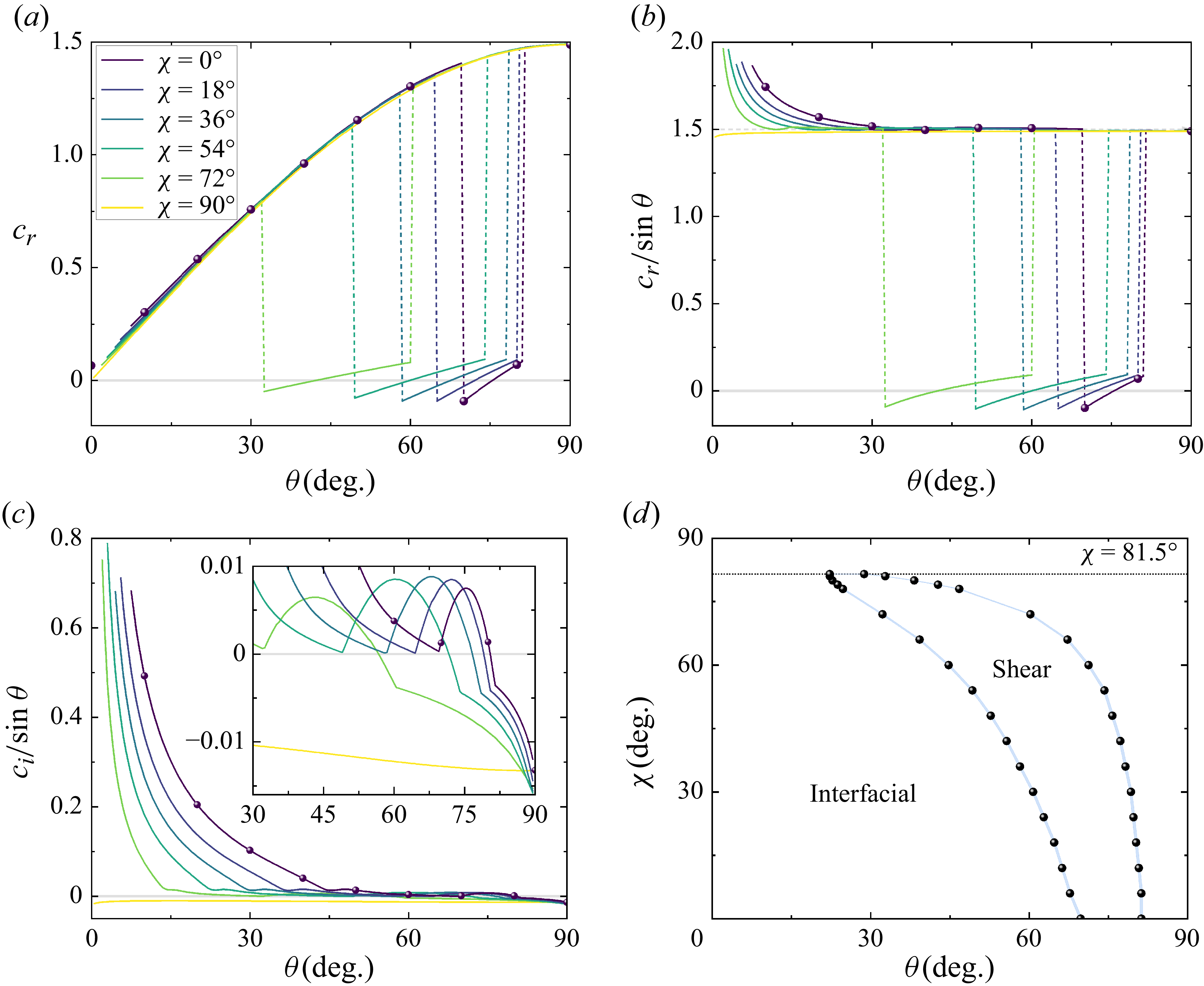
, figure 10
 $(a)$
illustrates the eigenvalue variation as a function of
 $\theta$
for varying
 $\chi$
. Other parameters are
 $\phi =45^\circ$
and
 $k=0.2,\ Re=20\,000$
, where shear-mode instability is possible. Data lines are reproduced by the mapping method of § 5.1, and a few direct solutions of OS equation (2.13) are plotted as symbols, showing consistency with the mapping results. The mapped data lines break up at relatively small
 $\theta$
values owing to the incompleteness of the solution set
 $c^*(\theta ^*,k,Re^*)$
, which can be evaluated given sufficient parameter space and resolution. For
 $c_{r,max}$
values, the
 $\chi =90^\circ$
variation is continuous while the other lines shows intermittent changes and drops to near zero. The step-like changes are ascribed to mode competition between interfacial and shear modes. For a more straightforward presentation,
 $c_{r,max}$
values are normalised by dividing by
 $\sin \theta$
so that the interfacial modes correspond to a unique base interfacial velocity
 $1.5$
, as shown in figure 10
 $(b)$
.
 $(a{-}c)$
Eigenvalue statistics against
 $\theta$
for varying perturbation angles
 $\chi$
. Lines indicate data obtained using mapping relation; symbols indicate data directly solved from the OS equation with
 $\chi =0^\circ$
.
 $(d)$
Phase diagram of dominant stability modes. Other parameters used are
 $m=n=r=2,\ \phi =45^\circ ,\ k=0.2,{} Re=20\,000$
.

Additionally,
 $c_{i,max}/ \sin \theta$
versus
 $\theta$
is shown figure 10
 $(c)$
. Stability with
 $\chi =90^\circ$
is fully dominated by interfacial modes, and stable for
 $0^\circ \leqslant \theta \leqslant 90^\circ$
. Shear instabilities generally exist for
 $0^\circ \leqslant \chi \lesssim 72^\circ$
, as denoted by regions with near-zero
 $c_{r,max}$
. For normalised
 $c_{i,max}$
values, shear-dominant regions correspond to the arched curve in the inset of figure 10
 $(c)$
. Discontinuities of
 $c_{r,max}$
and derivatives of
 $c_{i,max}$
are found when the dominant mode changes. Figure 10
 $(d)$
plots the phase diagram of dominant modes. For
 $\chi =0^\circ$
, the parameter space of
 $69.75^\circ \lesssim \theta \lesssim 81.25^\circ$
is dominated by shear modes. As
 $\chi$
increases, the shear-mode-dominant parameter space shifts towards smaller
 $\theta$
. For 3-D perturbations with
 $\chi =72^\circ$
, this corresponds to
 $32.25^\circ \lesssim \theta \lesssim 60.25^\circ$
, which can be ascribed to shear instability induced by Poiseuille flow perturbed in the
 $z$
direction.
 $(a)$
Ratio between the rate of work done in deforming the interface and the total viscous dissipation rate (details in supplementary material § 1), with the subscripts
 $1,2$
for upper and lower layers, respectively.
 $(b)$
Ratio between the rate of work done in deforming the interface and the total production rate. Other parameters used are
 $m=n=r=2,\ \phi =45^\circ ,\ k=0.2,\ Re=20\,000$
.

To elucidate the underlying physical mechanisms, corresponding perturbation energy contributions
 $\chi =0^\circ ,18^\circ$
are plotted in figure 11. Referenced to Boomkamp & Miesen (Reference Boomkamp and Miesen1996), for the typical Yih-type instability, which is presently considered as an interfacial instability, the energy transfer is driven by the rate of work done in deforming the interface. Thus to show the energetic differences of interfacial and shear instability, we plot the logarithm of the fraction of the interfacial work term relative to the total energy dissipation and production in figure 11
 $(a{,}b)$
, respectively. For shear instabilities, the relative magnitude of interfacial work term is approximately
 $O(10^{-3})$
, while elsewhere it approaches
 $O(10^{-1})$
and even larger.
5.3. The 3-D base flow: the orientational angle
$\phi$

When
 $\phi =0^\circ$
, the mean flow is parallel to the wall velocity vector, and the base flow degenerates to a 1C-1D, PCP form. As
 $\phi$
increases, there exists a Poiseuille component in the
 $z$
direction forming a 2C-1D base flow configuration. Here, we consider the effect of the orientational angle
 $\phi$
under stratification parameters
 $m=n=r=2$
, and stability modes are further discussed.
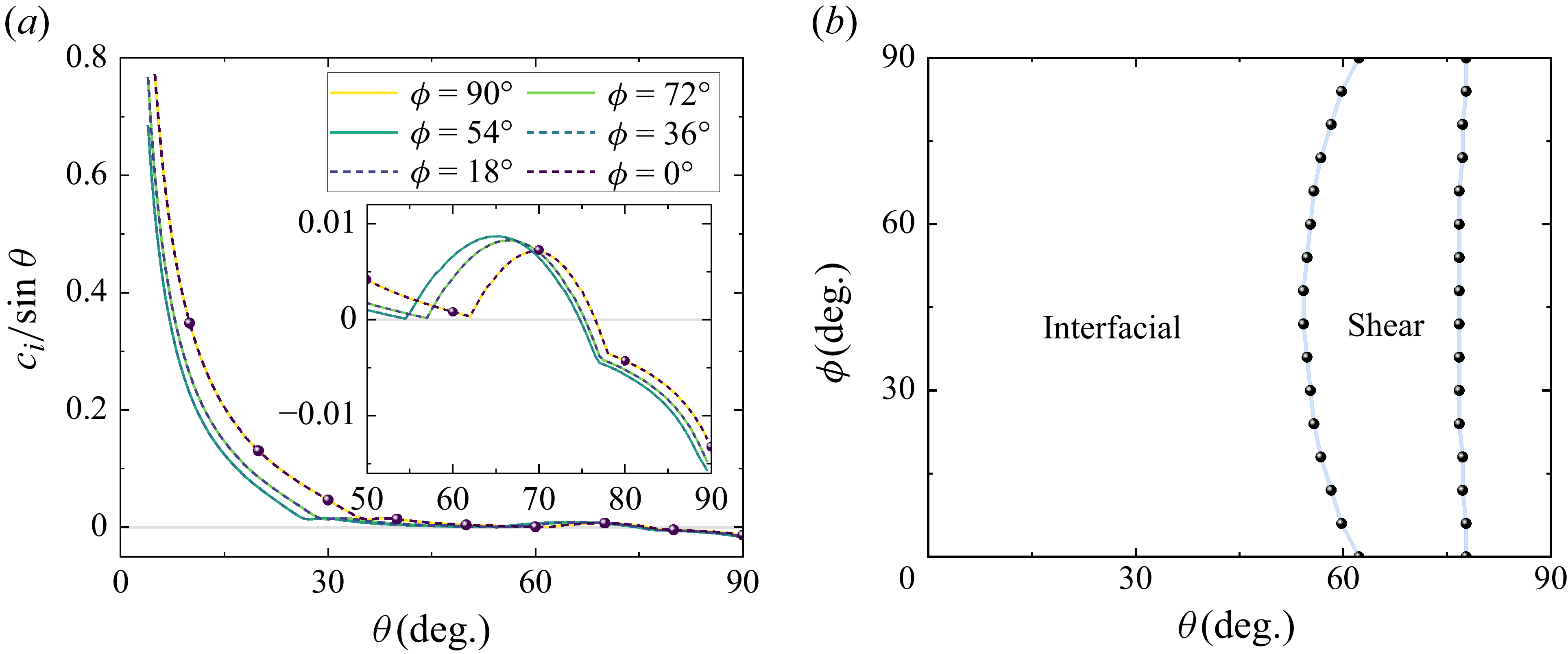
 $(a)$
Normalised
 $c_{i,max}$
values against
 $\theta$
for varying orientational angles
 $\phi$
. Lines indicate data obtained using the mapping relation; symbols indicate data directly solved from the OS equation with
 $\phi =0^\circ$
.
 $(b)$
Phase diagram of dominant stability modes. Other parameters used are
 $m=n=r=2,\ \chi =45^\circ ,\ k=0.2,{} Re=20\,000$
.

In the mapping equations (see § 2.5) from GCP to PCP, we recall that
 $\phi$
is absorbed in the factor
 $\cos (\phi -\chi )$
, and only functions in this form. This further leads to the symmetric solutions for eigenvalues
 $c(\phi ;\theta _0, \chi _0, k_0, {\textit{Re}}_0)$
about
 $\phi =\chi _0$
(values with subscripts are fixed), which gives
 \begin{equation} c(\phi ;\, \theta _0, \chi _0, k_0, {\textit{Re}}_0) = c(2\chi _0 - \phi ;\, \theta _0, \chi _0, k_0, {\textit{Re}}_0). \end{equation}
In figure 12, we choose
 $\chi =45^\circ$
and
 $k=0.2,\ Re=20\,000$
, and plot the normalised
 $c_{i,max}$
against
 $\theta$
. As indicated by (5.2), symmetry about
 $\chi =45^\circ$
is observed. Specifically, data lines of cases with two complementary angles coincide, such as
 $\phi =0^\circ$
and
 $\phi =90^\circ$
. For different
 $\phi$
values, interfacial and shear instabilities are observed, denoted by the derivative discontinuity of
 $c_{i,max}$
, shown in the inset of figure 12
 $(a)$
. The first mode change happens in the unstable region, as the interfacial
 $c_{i,max}$
value continues to decrease below that of the shear mode. When the values further decrease, the second mode change occurs between the stable shear and interfacial modes. Characteristics of
 $c_{r,max}$
resemble the previous plots with varying
 $\chi$
(figure 10
a,b), where step-like changes distinguish the two modes. Figure 12
 $(b)$
plots the phase diagram. The shear-dominant parameter space is symmetric about
 $\chi =45^\circ$
, with an upper limit at approximately
 $\theta =77^\circ$
. From an energetic perspective, the relative quantities of interfacial work are plotted in figure 13. Representative examples of
 $\phi =0^\circ$
and
 $18^\circ$
are plotted. For the shear-mode instability, the relative work done by the deforming interface manifests a magnitude of approximately
 $O(10^{-3})$
. This energy distribution plot is consistent with the interfacial–shear phase diagram results presented in figure 12
 $(b)$
, and it further validates the effectiveness of the mapping procedure.
 $(a)$
Ratio between the rate of work done in deforming the interface and the total viscous dissipation rate (details in supplementary material § 1), with the subscripts
 $1,2$
for upper and lower layers, respectively.
 $(b)$
Ratio between the rate of work done in deforming the interface and the total production rate. Other parameters used are
 $m=n=r=2,\ \chi =45^\circ ,\ k=0.2,\ Re=20\,000$
.

6. Conclusion
We have studied the linear instability of the two-layer GCP system, defined by a steady, two-velocity-component base flow with wall-normal variation between two parallel plates. Specifically, two immiscible fluids are considered with depth ratio
 $n$
and with viscosity ratio
 $m$
and density ratio
 $r$
, contained between the two moving plates. The flow is driven by both relative plate movement and an externally applied pressure gradient vector along an angle
 $0^\circ \leqslant \phi \leqslant 90^\circ$
to the plates’ relative velocity vector, with magnitude ratio
 $\cos \theta$
(
 $0^\circ \leqslant \theta \leqslant 90^\circ$
). The base flow is thus determined by
 $(\theta ,\phi ,{\textit{Re}}_1)$
together with
 $(m,n,r)$
, with
 ${\textit{Re}}_1$
the Reynolds number based on fluid 1 (the upper fluid). The extended OS and Squire equations are derived for 3-D small perturbations with resultant wavenumber
 $k$
and perturbation front angle
 $\chi$
. An eight-parameter eigenvalue problem results with eigenvalue
 $c=c(\theta ,\phi ,\chi ,k, {\textit{Re}}_1;m,n,r)$
.
A mapping is found to transform the 3-D perturbative GCP problem to a 2-D perturbation for a PCP problem, thus simplifying to a six-parameter problem
 $c^*=c^*(\theta ^*,k, Re^*_1;m,n,r)$
. For the overall two-layer stability problem, because the inverse problem of finding a minimal unstable Reynolds number is not the primary purpose of the present study, use of this mapping can significantly decrease the complexity of determining neutral surfaces in the multi-parameter space.
To provide an explicit guide for dividing the stable/unstable regions for GCP stability, following Yih (Reference Yih1967), a long-wave analysis assuming small wavenumber
 $k\ll 1$
is conducted, in which the first-order eigenvalue
 $c_1$
is obtained in the form of a product of three polynomials. Three neutral surfaces, with the first in terms of
 $m$
only, the second with
 $(m,n)$
, and the third as a function of
 $m$
,
 $n$
and
 $r$
, are discussed in detail. Interfacial mode instabilities, associated with the presence of a two-layer viscosity interface, provide the mechanism for neutral-surface partition of the parameter space into stable/unstable regions.
To elucidate understanding of instability modes, the Cowley & Smith (Reference Cowley and Smith1985) long-wave asymptotic analysis is adapted to explore the limiting regime of shear instability. Cut-off or critical values of
 $\theta$
can be deduced from the numerical solution to (4.1). For a typical PCP case
 $m=n=r=2$
, we have
 $\theta _c=57.10^\circ$
, below which shear mode is stable. This value is smaller than the reversal angle
 $\theta _r$
, with the result that the cut-off phenomenon is somewhat obscured. Further, for varying
 $m$
and
 $r$
, competition between the reversal and the cut-off phenomena lead to complex neutral surface geometries. Where
 $\theta \gt \theta _c$
, for unstable regions, the shear mode dominates stability at relatively small wavenumbers. In another specific case,
 $m=n=0.5,\ r=1$
, a unique type of instability mode is detected, which is transported at approximately the interfacial velocity, and is interpreted as the viscous boundary layer mode regime proposed by Hooper & Boyd (Reference Hooper and Boyd1987).
Finally, we provide a general discussion for the GCP stability problem, with focus on the effect of pressure-gradient flow angle
 $\phi$
and the perturbation front angle
 $\chi$
. General features of GCP cases are presented with the example case
 $m=n=r=2$
for
 $k=0.2,\ {\textit{Re}}_1=20\,000$
, with good consistency between the mapping method and the numerical solution. Dominant instability modes are observed to shift between interfacial and shear modes as
 $\theta$
varies from
 $0^\circ$
to
 $90^\circ$
.
Supplementary material
Supplementary material is available at https://doi.org/10.1017/jfm.2025.10897.
Funding
This work was supported by the National Natural Science Foundation of China (nos 12388101, 12172352), the Strategic Priority Research Programme of the Chinese Academy of Sciences (no. XDB0500300) and the National Key R&D Programme of China (no. 2022YFA1005200).
Declaration of interests
The authors report no conflict of interest.
Appendix A. On Squire modes and rationality of OS-based mapping
Squire modes are defined as eigenvalues solved from Squire equations, which are proven to be damped. In the framework of two-layer GCP flow, we follow Schmid & Henningson (Reference Schmid and Henningson2001) by taking the imaginary part of (2.14), which gives
 \begin{align} c_{i,{\textit{Squire}}} \int _{0}^{1} |\eta _1|^2 \, \mathrm{d}y &= \frac {-1}{\alpha _1\, {\textit{Re}}_1}\, \text{Re}[\eta _1^*(0)\, D\eta _1(0)] - \frac {1}{\alpha _1\, {\textit{Re}}_1} \int _{0}^{1} \big ( |D\eta _1|^2 + k^2 |\eta _1|^2 \big ) \,\mathrm{d}y, \end{align}
 \begin{align} c_{i,{\textit{Squire}}} \int _{-n}^{0} |\eta _2|^2 \, \mathrm{d}y &= \frac {1}{\alpha _1\, {\textit{Re}}_2} \text{Re}[\eta _2^*(0)\, D\eta _2(0)] - \frac {1}{\alpha _1\, {\textit{Re}}_2} \int _{-n}^{0} \big ( |D\eta _2|^2 + k^2 |\eta _2|^2 \big )\, \mathrm{d}y, \end{align}
where
 $\text{Re}$
denotes taking the real part. Referring to Mohammadi & Smits (Reference Mohammadi and Smits2017), when dealing with Squire modes, ordinary solutions of OS equation
 $v_i=0\ (i=1,2)$
are quoted, which leads to the simplification of (2.20) and (2.21):
 \begin{align} \eta _{1}(0)&=\eta _{2}(0), \end{align}
 \begin{align} D \eta _{1}(0) &= m\, D \eta _{2}(0). \end{align}
Recalling that
 ${\textit{Re}}_2 = {\textit{Re}}_1\, r/m$
, the following equation can be derived:
 \begin{align} &c_{i,{\textit{Squire}}} \left ( \frac {1}{r} \int _{0}^{1} |\eta _1|^2 \, \mathrm{d}y + \int _{-n}^{0} |\eta _2|^2 \, \mathrm{d}y \right ) \nonumber \\ &\quad =-\frac {1}{r} \frac {1}{\alpha _1\, {\textit{Re}}_1} \int _{0}^{1} \left ( |D\eta _1|^2 + k^2 |\eta _1|^2 \right ) \mathrm{d}y - \frac {1}{\alpha _1\, {\textit{Re}}_2} \int _{-n}^{0} \left ( |D\eta _2|^2 + k^2 |\eta _2|^2 \right ) \mathrm{d}y. \end{align}
Since the Squire modes are always damped, a solution of the OS equation is sufficient for the stable/unstable criterion, and also supports the mapping method that aims to provide rapid and general instability features.
Appendix B. Numerical method and verification
The D2-method proposed by Dongarra, Straughan & Walker (Reference Dongarra, Straughan and Walker1996) is adopted in present study, in which an intermediate function
 $\xi _i=(D^2-k^2)v_i$
is employed to reduce the order of the extended OS–Squire equations (2.13) and (2.15) to avoid a possible ill-conditioned matrix problem. We can rewrite the system of equations as
 \begin{align} (D^2-k^2)v_i - \xi _i &= 0, \end{align}
 \begin{align} - {v}_i {D}^2{U_{P,i}} + \frac { i \big ({D}^2-k^{2}\big )\xi _i}{{k} \cos (\phi -\chi )\, {\textit{Re}}_i}+ \left [ U_{P,i} + \frac {\cos \chi }{\cos (\phi -\chi )} \, U_{C,i} \right ] \xi _i &= {c} \xi _i, \end{align}
 \begin{align} - {v}_i X_i + \frac { i \big ({D}^2-k^{2}\big )\eta _i}{{k} \cos (\phi -\chi )\, {\textit{Re}}_i} + \left [ U_{P,i} + \frac {\cos \chi }{\cos (\phi -\chi )} \, U_{C,i} \right ] \eta _i &= c \eta _i, \end{align}
with
 \begin{equation} X_i = \tan (\phi -\chi ) {D}{U_{P,i}} - \frac {\sin \chi }{\cos (\phi -\chi )}\, {D}{U_{C,i}} . \end{equation}
The computational domain is mapped to
 $(-1,1)$
for each fluid layer by the transformation
 \begin{equation} z_1 = 2y_1-1 \quad \text{for} \quad 0\leqslant y_1 \leqslant 1, \qquad z_2 = -\frac {2}{n}y_2-1 \quad \text{for} \quad {-n}\leqslant y_2 \leqslant 0, \end{equation}
to let
 $z_i=1$
for the moving wall boundaries, and
 $z_i=-1$
for the fluid interface.
The order-reduced system is then discretised using a Chebyshev-tau QZ algorithm. The six variables
 $(v_1, \xi _1, \eta _1, v_2, \xi _2, \eta _2)$
are expanded in Chebyshev polynomials. Taking
 $v_1$
for an example, we have
 $v_1=\sum _{n=0}^{N}a_{v_1,n}\, T_n(y)$
, with
 $y_j=\cos (j\unicode{x03C0} /N)$
,
 $a_{v_1,n}$
the coefficient of the
 $n$
th Chebyshev polynomial, and
 $T_n(y)=\cos (n\, {\cos }^{-1} y)$
. The order-reduced system can be seen as a generalised eigenvalue problem
 $\unicode{x1D63C} \boldsymbol{a} =c \unicode{x1D63D} \boldsymbol{a}$
, with
 $\boldsymbol{a} = (a_{v_1,n}, a_{\xi _1,n}, a_{\eta _1,n}, a_{v_2,n}, a_{\xi _2,n}, a_{\eta _2,n})$
, resulting in a matrix of size
 $6(N+1)\times 6(N+1)$
. For boundary conditions, the ‘boundary-boarding’ strategy (Boyd Reference Boyd2001) is adopted, in which
 $12$
rows of the pseudo-spectral matrices are directly replaced by boundary conditions.
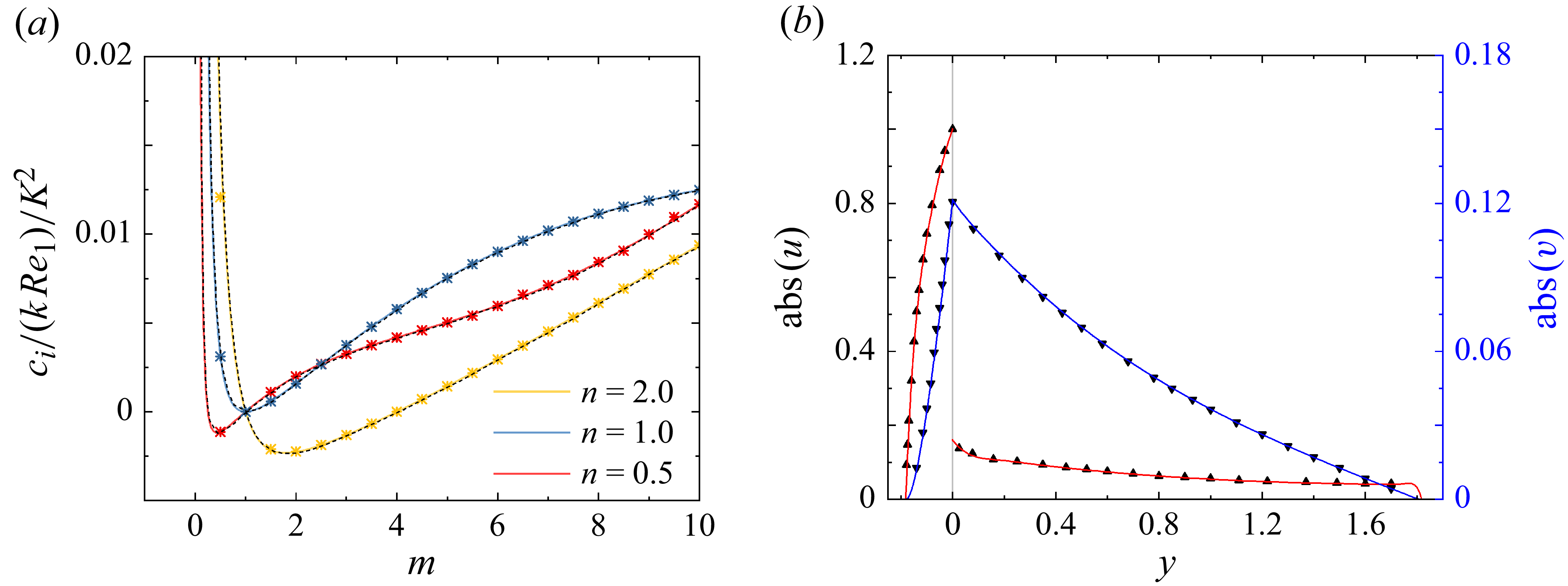
Code validation. (
 $a$
) Evolution with the viscosity ratio of the normalised
 $c_i$
, with
 $r=1$
,
 $\theta =90^\circ$
,
 $\phi =0^\circ$
, where gravity and surface tension are neglected. Here,
 $K=(n^2+n)/(m+n)$
is the ratio of reference velocities in the present study and Yiantsios & Higgins (Reference Yiantsios and Higgins1988). Symbols indicate numerical results; solid lines indicate long-wave analysis of (3.8); dashed lines indicate data from Yiantsios & Higgins (Reference Yiantsios and Higgins1988). (
 $b$
) Perturbation
 $u(y),v(y)$
for two-layer Couette flow, normalised by
 $|u_2|_{{\textit{max}}}$
. Solid lines indicate present results. Symbols indicate data from Mohammadi & Smits (Reference Mohammadi and Smits2017).

To calculate the eigenvalues,
 $N\gtrsim 100$
is used. The parameter
 $N$
is carefully chosen to ensure that the maximum relative error of
 $c_i$
, the imaginary part of the eigenvalues, for the five least stable modes is below
 $10^{-5}$
. For a better resolution of eigenvectors
 $\boldsymbol{a}$
, we carry out a Rayleigh quotient iteration for a specific eigenvalue. The procedure reduces the residual error
 $\| \unicode{x1D63C} \boldsymbol{a} - c \unicode{x1D63D} \boldsymbol{a} \|$
to
 $10^{-10}$
, and is proven to be
 $N$
-irrelevant.
The code verification for the single-layer GCP flow can be found in Cheng et al. (Reference Cheng, Ma, Pullin and Luo2024). For the two-layer stability problem, the stratified PP case (
 $\phi =0^\circ ,\ \theta =90^\circ $
) is employed for eigenvalue verification as shown in figure 14
 $(a)$
. The lines represent the long-wave results from § 3, while symbols denote the numerical results. The present numerical results agree well with both the previous studies by Yiantsios & Higgins (Reference Yiantsios and Higgins1988) and the long-wave analysis. For eigenvector validation, we solve the OS–Squire system at
 $m=0.5,\ n=0.1, r=1$
following the two-layer Couette flow investigation by Mohammadi & Smits (Reference Mohammadi and Smits2017). Results are shown in figure 14
 $(b)$
. The present perturbation magnitudes reasonably match the literature data.
Appendix C. Details of
$\boldsymbol{O(1)}$
and
$\boldsymbol{O(k)}$
expansions in long-wave analysis


C.1. The
$O(1)$
boundary conditions

For
 $O(1)$
(3.2) in long-wave analysis, wall boundary conditions are given by
 \begin{align} v_{1,0}|_{y=1}&=v_{2,0}|_{y=-n}=0, \end{align}
 \begin{align} Dv_{1,0}|_{y=1}&=Dv_{2,0}|_{y=-n}=0. \end{align}
At the fluid surface, equations for the continuity of perturbation velocity
 $v$
, the shear and normal stress are significantly simplified as
 \begin{align} v_{1,0}|_{y=0} &=v_{2,0}|_{y=0}, \end{align}
 \begin{align} D^2 v_{1,0}|_{y=0} &= m\!D^2 v_{2,0}|_{y=0}, \end{align}
 \begin{align} D^3 v_{1,0}|_{y=0} &= m\!D^3 v_{2,0}|_{y=0}. \end{align}
The leading-order perturbation velocity
 $v_{i,0}(y)$
is obtained by solving (3.2), subject to the boundary conditions specified above. Noted that
 $c_0$
is not involved in the equations above, while it emerges in the simplified form of (2.19), given by
 \begin{equation} \varDelta \left [ Dv_{i,0} - \frac { \cos (\phi -\chi ) \sin \theta \, D U_{P,i} + \cos \chi \cos \theta \, D U_{C,i} } { \cos (\phi -\chi ) \left ( \sin \theta \, U_{P,i}-c_0 \right ) + \cos \chi \cos \theta \, U_{C,i} } v_{i,0} \right ] = 0 \quad \mathrm{at}\ y=0. \end{equation}
The phase speed
 $c_0$
is then determined by substituting
 $v_{i,0}(y)$
into (C6).
C.2. The
$O(k)$
boundary conditions and relevant coefficients

At
 $O(k)$
, wall boundary conditions are given by
 \begin{align} v_{1,1}|_{y=1}&=v_{2,1}|_{y=-n}=0, \end{align}
 \begin{align} Dv_{1,1}|_{y=1}&=Dv_{2,1}|_{y=-n}=0. \end{align}
The continuity equations of perturbation velocity
 $v$
and shear stress are expressed in the same form as (C3) and (C4), but with
 $v_{i,1}$
:
 \begin{align} v_{1,1}|_{y=0} &=v_{2,1}|_{y=0}, \end{align}
 \begin{align} D^2 v_{1,1}|_{y=0} &= m D^2 v_{2,1}|_{y=0}. \end{align}
For the normal stress, the equation is expressed as
 \begin{eqnarray} & & \varDelta \Bigg [ \frac {\rho _i}{\rho _1} \left ( \sin \theta \, DU_{P,i} + \frac {\cos \chi }{\cos (\phi -\chi )} \cos \theta \, DU_{C,i} \right ) v_{i,0} \nonumber \\ & &\quad - \frac {\rho _i}{\rho _1} \left ( \sin \theta \, U_{P,i} + \frac {\cos \chi }{\cos (\phi -\chi )} \cos \theta \, U_{C,i} - c_0\right ) D v_{i,0} -\frac {\mu _i}{\mu _1} \, \frac {i\! D^3 v_{i,1}}{{\textit{Re}}_1 \cos (\phi - \chi )} \Bigg ] \nonumber \\ & & = \frac {\textit{Fr}\, v_{i,0}}{\cos ^2(\phi - \chi ) \big ( \sin \theta \, U_{P,i} + \big({\cos \chi }/{\cos (\phi -\chi )}\big) \cos \theta \, U_{C,i} - c_0\big ) } \quad \mathrm{at}\ y=0. \end{eqnarray}
The continuity equations for
 $u,w$
are rearranged and given by
 \begin{eqnarray} && \varDelta \Bigg [ \left ( \sin \theta \, U_{P,i} + \frac {\cos \chi }{\cos (\phi -\chi )} \cos \theta \, U_{C,i} - c_0\right )Dv_{i,1} - c_1 Dv_{i,0}\nonumber \\ && {}\quad -\left ( \sin \theta \, DU_{P,i} + \frac {\cos \chi }{\cos (\phi -\chi )} \cos \theta \, DU_{C,i} \right ) v_{i,1} \Bigg ]=0 \quad \mathrm{at}\ y=0. \end{eqnarray}
The unknown
 $c_1$
appears exclusively in (C12), and is subsequently determined using the same strategy as for
 $c_0$
, by substituting
 $c_0$
,
 $v_{i,0}$
and
 $v_{i,1}$
into (C12).
Corresponding coefficients used in (3.8) are
 \begin{align} H_1 &= 14m^7 (4 n+1)-56m^6 n \big (4 n^3+3 n^2-5 n-1\big ) \nonumber \\ &\quad -14m^5 n^2 \big (32 n^5-96 n^4 r+136 n^4-196 n^3 r+228 n^3-135 n^2 r+114 n^2 \nonumber \\ &\quad -\,32 n r-36 n-8\vphantom{14m^5}\big ) \nonumber \\ &\quad -56m^4 n^4 \!\big (2 n^4 r+14 n^4\!-49 n^3 r+61 n^3\!-95 n^2 r+95 n^2\!-61 n r+49 n-\!14 r\!-\!2\big ) \nonumber \\ &\quad -14m^3 n^5 \big (8 n^5 r+36 n^4 r+32 n^4-114 n^3 r+135 n^3-228 n^2 r+196 n^2-136 n r \nonumber \\ &\quad +\,96 n-32 r\vphantom{14m^5}\big ) \nonumber \\ &\quad -56m^2 n^8 r \big (n^3+5 n^2-3 n-4\big )-14mn^{11} r \big (n+4\big ), \end{align}
 \begin{align} H_2&= m^7 (6 n+1)-m^6 n \big (88 n^3+120 n^2+9 n+2\big ) \nonumber \\ &\quad+m^5 n^2 \big (224 n^5+672 n^4 r+424 n^4+1486 n^3 r-60 n^3+1043 n^2 r-222 n^2 \nonumber \\ &\quad +\,224 n r+120 n+32\vphantom{14m^5}\big ) \nonumber \\ &\quad+m^2 n^7 \big (32 n^5 r+120 n^4 r+224 n^4-222 n^3 r+1043 n^3-60 n^2 r+1486 n^2 \nonumber \\ &\quad +\,424 n r+672 n+224 r\vphantom{14m^5}\big ) \nonumber \\ &\quad+m n^{10} r\big (2 n^3+9 n^2+120 n+88\big )+ m^4 n^4 J_1 + m^3 n^5 J_2 +n^{14} r+6 n^{13} r, \end{align}
 \begin{align} F_1 &= 420 m^2 (m+n)^2 \big (n^4 + 4n^3 m +6n^2 m + 4mn + m^2\big )^3, \end{align}
with coefficients
 $J_1,\,J_2$
used in
 $H_2$
given by
 \begin{align} J_1 &= 224 n^5-272 n^4 r+1512 n^4+1080 n^3 r+2344 n^3 + 3021 n^2 r+646 n^2 \nonumber \\ &\quad +2086 n r-444 n+392 r+16, \end{align}
 \begin{align} J_2 &= 16 n^5 r+392 n^5-444 n^4 r+2086 n^4+646 n^3 r +3021 n^3+2344 n^2 r \nonumber \\ &\quad + 1080 n^2+1512 n r-272 n+224 r. \end{align}
Note that
 $H_1$
and
 $H_2$
are functions of
 $(m,n,r)$
, while
 $F_1=F_1(m,n)$
.
Appendix D. Boundary conditions for Cowley-type long-wave analysis
Following Cowley & Smith (Reference Cowley and Smith1985), a parameter
 $\lambda _i$
is introduced in two-layer GCP flow under a long-wave approximation
 $k\rightarrow 0$
:
 \begin{equation} \lambda _i = (k\, {\textit{Re}}_i)^{-1},\quad i=1,2. \end{equation}
Neglecting the higher order
 $O(k^2)$
, the OS equation can be simplified as
 \begin{equation} \left [ \left (U_{P,i} \sin \theta -{c}\right ) + \frac {\cos \chi \cos \theta }{\cos (\phi -\chi )} \, U_{C,i} \right ] {D}^2 v_i - {v}_i \sin \theta \, {D}^2{U_{P,i}}= \frac {\lambda _i\, {D}^4 v_i}{i \cos (\phi -\chi ) }. \end{equation}
The corresponding boundary conditions are treated with the same strategy. The equations for solid wall conditions stay unchanged:
 \begin{eqnarray} v_{1}|_{y=1}=Dv_{1}|_{y=1}=v_{2}|_{y=-n}=Dv_{2}|_{y=-n}&=&0. \end{eqnarray}
And continuity of perturbation velocity at the interface gives
 \begin{align} \varDelta \left [v_i\right ]&=0, \end{align}
 \begin{align} \varDelta \left [ Dv_i - \frac { \cos (\phi -\chi ) \sin \theta \, D U_{P,i} + \cos \chi \cos \theta \, D U_{C,i} } { \cos (\phi -\chi ) \left ( \sin \theta \, U_{P,i}-c \right ) + \cos \chi \cos \theta \, U_{C,i} } v_i \right ] &= 0. \end{align}
For the shear stress continuity,
 \begin{eqnarray} \varDelta \left [ \frac {\mu _{i}}{\mu _1}\, D^2 v_i \right ] &=&0. \end{eqnarray}
Normal stress continuity is rearranged as
 \begin{align} &\varDelta \Bigg [ \frac {\rho _{i}}{\rho _1} \left (\left ( \sin \theta\, DU_{P,i} + \frac {\cos \chi }{\cos (\phi -\chi )} \cos \theta\, DU_{C,i} \right )v_i \right . \nonumber \\ &\quad \left .- \left ( \sin \theta\, U_{P,i} + \frac {\cos \chi }{\cos (\phi -\chi )} \cos \theta \, U_{C,i} -c \right ) Dv_i \right ) \nonumber \\ &\quad - \frac {\rho _{i}}{\rho _1} \, \frac {i \lambda _i\, D^3 v_i }{ \cos \left (\phi -\chi \right ) } \Bigg ] = \frac {ik \left ( Fr\, \delta + {We}^{-1}\,R^{-1} \right ) }{\cos \left (\phi -\chi \right )}. \end{align}
Equation set (4.1) is now complete and solvable. Only two parameters,
 $\lambda _i$
and
 $\theta$
, are involved if gravity and surface tension are neglected.