1 Introduction
Air traffic has been in almost constant progress, with a yearly average increase of 5 %, during the past 50 years and will continue to grow as a consequence of the democratization of air transport in many parts of the world (Airbus SAS 2015). Among other issues, the increase in the number of flights has led to the saturation of major airports, especially at peak hours. In that context, separation distances imposed to mitigate the risk of wake vortices encountered at take-off and landing appear to be an important factor to play with in order to increase the frequency of arrivals/departures. The goal is to improve airport capacity without building new infrastructures, which is often impossible for technical, environmental or societal reasons. In the present work, we propose a new vortex mitigation strategy based on flow control applied at the ground. The action of control gives novel insight into the mechanisms affecting vortex evolution in ground effect and how these can be manipulated.
For an inviscid flow (Lamb Reference Lamb1932) a pair of rectilinear counter-rotating vortices set parallel to the ground in a quiescent environment moves along hyperbolic trajectories. The initial descent is related to the downward momentum provided to the flow by the lifting surface. The subsequent lateral displacement is the consequence of the momentum induced by the image vortices about the ground. With viscosity, the phenomenon of vortex rebound occurs, as reported by Dee & Nicholas (Reference Dee and Nicholas1968), i.e. the vortex leaves the hyperbolic trajectory, gains relative altitude and features little sideward motion. From an air traffic management perspective, this corresponds to a persistence of the vortices about the runway. As a consequence of the pragmatic importance of this matter and the required fundamental knowledge of vortex dynamics and turbulence near walls, vortex rebound has received much attention in the past. Following Harvey & Perry (Reference Harvey and Perry1971), vortex rebound results from the formation of a detached boundary layer at the ground, the former being formed due to the velocity field induced by the vortices, and the generation of opposite sign vorticity. The production of this secondary vorticity at the wall during the dipole–wall collision was in particular studied by Coutsias & Lynov (Reference Coutsias and Lynov1991) and Clercx & Van Heijst (Reference Clercx and Van Heijst2002). Barker & Crow (Reference Barker and Crow1977) explained vortex rebound as the elliptic deformation of the vortex as it nears the ground, with the subsequent oscillation of the ellipticity creating the vertical motion of the vortex centre. In Peace & Riley (Reference Peace and Riley1983), a matched asymptotic expansion of the vortex induced boundary layer shows that the increase of vortex height is also to be attributed to the thickness effect associated with the developing transverse boundary layer. The rebound has been simulated by Orlandi (Reference Orlandi1990), Coutsias & Lynov (Reference Coutsias and Lynov1991), Zheng & Ash (Reference Zheng and Ash1996), Türk, Coors & Jacob (Reference Türk, Coors and Jacob1999) and Clercx & Van Heijst (Reference Clercx and Van Heijst2002). Zheng & Ash (Reference Zheng and Ash1993) used a specific vorticity–streamfunction computational method, a technique that allows for efficient calculation of the flow evolution, up to large Reynolds numbers (Zheng & Ash Reference Zheng and Ash1996; Türk et al. Reference Türk, Coors and Jacob1999).
The inviscid dynamics of the vortex pair would be beneficial to the airport problem. Indeed, the presence of viscosity, due to the induced boundary layer and entrainment effect associated with secondary vorticity, results in a dramatic persistence of the vortices below the flight path that strongly constrains the possibility for reduced separation distances between aircraft. This naturally suggests that a control aimed at removing the effect of viscous friction at the wall would be beneficial. Following this simple idea, the present work looks at how to apply blowing/suction of air at the wall to favour an improved lateral displacement of trailing vortices approaching ground. A previous work to control wake vortices at the ground is described in Holzäpfel et al. (Reference Holzäpfel, Stephan, Heel and Körner2016) and uses a system of plate lines developed in a heuristic way.
It is noteworthy that the dynamics of vortices in ground effect generally results from multiple other effects, notably cross-wind, stratification, turbulence and three-dimensionality (Robins & Delisi Reference Robins and Delisi1993; Zheng & Ash Reference Zheng and Ash1996; Gerz, Holzäpfel & Darracq Reference Gerz, Holzäpfel and Darracq2002; Pailhas, de Saint & Touvet Reference Pailhas, de Saint and Touvet2002; Harris & Williamson Reference Harris and Williamson2012; Bricteux et al. Reference Bricteux, Duponcheel, De Visscher and Winckelmans2016; Leweke, Le Dizes & Williamson Reference Leweke, Le Dizes and Williamson2016). Gentle side wind is in particular known to be particularly harmful for the persistence of wake vortices (Gerz et al. Reference Gerz, Holzäpfel and Darracq2002). In the current study, which targets the numerical implementation of the control and its application to the most simple case, none of these effects are accounted for. The resulting scenario, two-dimensional laminar vortices in a quiescent environment, is yet one of the worst cases for air traffic and consequently quite conservative since turbulence, stratification and three-dimensional effects all lead to an accelerated dissipation of the vortex system. The limitation to a two-dimensional physical set-up amounts to considering infinite trailing vortices, parallel to the ground.
Irrespective of aircraft wakes, vortices are elementary components of wall turbulence. The understanding of vortex/ground interaction is therefore of primary interest for all turbulent flows and flow control in this domain could play an interesting role in accomplishing objectives such as drag reduction, relaminarization, delay of flow separation and mixing enhancement. A significant part of the drag generated by wall turbulence results from the shear stress powered by coherent streamwise vortices located near the wall (Kravchenko, Choi & Moin Reference Kravchenko, Choi and Moin1993). The dynamics of these vortices includes sweep and lift (rebound) motions that resemble those of the large scale trailing vortices shed by airplanes. The typical Reynolds number involved is in the range  $O(10^{2}{-}10^{3})$. These vortices play an active part in the generation of turbulence at its early stages, by promoting longitudinal velocity streaks and the formation of secondary vorticity, whose destabilization leads the turbulence cycle. Conversely, their attenuation is able to trigger flow relaminarization (Jiménez & Pinelli Reference Jiménez and Pinelli1999). In developed wall turbulence Lee et al. (Reference Lee, Kim, Babcock and Goodman1997) and Choi, Moin & Kim (Reference Choi, Moin and Kim1994) show that the application of a blowing/suction control strategy produces significant drag and turbulence reduction by modifying the vortex lateral and vertical motions. Along this line Koumoutsakos (Reference Koumoutsakos1997) developed a sensor-based control strategy with mass exchange at the wall to manipulate wall vorticity. Vortex annihilation could even be attained this way. Akhavan, Jung & Mangiavacchi (Reference Akhavan, Jung and Mangiavacchi1993) realized control by lateral blowing and oscillatory wall deformation and also observes that this shifts the vortices and in turn reduces turbulence production. In all these studies it seems that reducing vortex rebound is a way to temper turbulent production. Such a feature could also be of interest to maintaining longitudinal vortices for longer times near the wall and controlling flow separation using vortex generators (Lin Reference Lin2002). One could also find interest in such controls for turbomachinery tip leakage vortex flow. Storer & Cumpsty (Reference Storer and Cumpsty1991) mentions that the tip leakage region leads to increased flow blockage and the tip vortex is a source of instabilities in the near stall regime (Furukawa et al. Reference Furukawa, Inoue, Saiki and Yamada1999).
The present work adopts an optimal control strategy, as detailed by Bewley (Reference Bewley2001) and Choi, Hinze & Kunisch (Reference Choi, Hinze and Kunisch1999), to do so. In the case when a large set of degrees of variables needs to be optimized, the associated direct–adjoint technique is particularly well suited. Here, the variable to be optimized is the velocity at the wall and falls into that category. The technique has been successfully applied for boundary layers and wakes (Walther, Airiau & Bottaro Reference Walther, Airiau and Bottaro2001; Homescu, Navon & Li Reference Homescu, Navon and Li2002; Airiau et al. Reference Airiau, Bottaro, Walther and Legendre2003; Guégan, Schmid & Huerre Reference Guégan, Schmid and Huerre2006; Flinois & Colonius Reference Flinois and Colonius2015). In Önder & Meyers (Reference Önder and Meyers2016), the optimal control method is used to improve the mixing of an incompressible axisymmetric jet and in Bewley, Moin & Temam (Reference Bewley, Moin and Temam2001) flow relaminarization and drag reduction in a plane channel are demonstrated. The control algorithm for an unsteady flow and nonlinear dynamics typically requires a large amount of storage as the full flow field information is needed at each time step. As a result, sub-optimal boundary control strategies have been designed to reduce the associated cost of computation. Such a strategy was for instance applied by Choi et al. (Reference Choi, Hinze and Kunisch1999) for the case of the recirculation bubble behind a backward-facing step. In the present study, linear interpolation is used to reduce this storage issue.
The paper is organized as follows. In § 2 we define the governing equations and present the numerical set-up to compute the dynamics of the vortices in ground effect. Section 3 presents the principal features of the uncontrolled flow. In § 4, we outline the optimal control approach that allows the maximization of the horizontal position of the vortices. In § 5 the strategy is applied, the various results are presented and we discuss the effect of optimal control on wake vortices. Conclusions and outlooks for application are provided in § 6.
2 Governing equations
In the following, the fluid domain is  $(x,y\geqslant 0)$ where
 $y=0$ is ground. The flow is started by a pair of counter-rotating Lamb–Oseen vortices, located at
 $(x_{c_{0}},y_{c_{0}})=(\pm 0.5b,y_{c_{0}})$ with initial circulation
 $\unicode[STIX]{x1D6E4}_{0}$. Initially the vortex dispersion radius that defines the vortex velocity profile is set to
 $a=0.15b$. Length and velocity are normalized on vortex separation
 $b$ and on the drift velocity of the vortex pair
 $v^{\ast }=\unicode[STIX]{x1D6E4}_{0}/2\unicode[STIX]{x03C0}b$, yielding a reference time
 $T^{\ast }=2\unicode[STIX]{x03C0}b^{2}/\unicode[STIX]{x1D6E4}_{0}$ and a circulation-based Reynolds number
 $Re=\unicode[STIX]{x1D6E4}_{0}/2\unicode[STIX]{x03C0}\unicode[STIX]{x1D708}$ where
 $\unicode[STIX]{x1D708}$ is the kinematic viscosity of the fluid. The Reynolds number is considered in the range
 $200\leqslant Re\leqslant 5000$. For the remainder of the paper and unless otherwise stated, all the quantities are normalized upon the aforementioned variables. The flow is governed by the incompressible Navier–Stokes equations,
 $$\begin{eqnarray}\left.\begin{array}{@{}l@{}}\unicode[STIX]{x1D735}\boldsymbol{\cdot }~\boldsymbol{u}=0,\\ \unicode[STIX]{x2202}_{t}\boldsymbol{u}+(\boldsymbol{u}\boldsymbol{\cdot }\unicode[STIX]{x1D735})\boldsymbol{u}=-\unicode[STIX]{x1D735}p+Re^{-1}\unicode[STIX]{x1D6FB}^{2}\boldsymbol{u},\\ \boldsymbol{u}(x,y=0,t)=\boldsymbol{u}_{w},\end{array}\right\}\end{eqnarray}$$
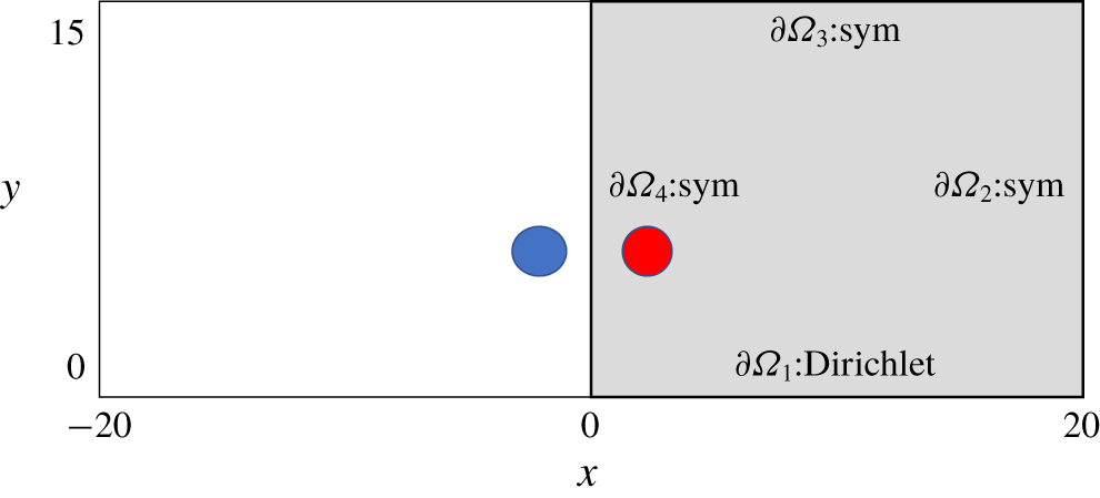
where  $\boldsymbol{u}_{w}$ is the velocity at the wall, which is zero in the uncontrolled case, and optimized in the controlled case. These equations are solved using the incompressible computational tool Nek5000 (Fischer, Lottes & Kerkemeier Reference Fischer, Lottes and Kerkemeier2008). Numerical simulations have been carried out using parallel computations with 128 cores and solving the set of (2.1) limited to the right half of the domain, denoted
 $\unicode[STIX]{x1D6FA}$, shown in figure 1 with a mesh containing
 $143\times 129=18\,447$ elements. Each element contains
 $8\times 8$ Gauss–Lobatto points, leading to 1.2 M discretization points. Boundary conditions are symmetry conditions at all frontiers except the wall where Dirichlet boundary condition is applied.
Schematic (not to scale) of the physical set-up. Dimensions are indicated. The right part of the domain is the computational domain and is shaded in grey. The disks represent the two Lamb–Oseen vortices at time  $t=0$. Symmetric conditions are applied at the right, upper and left boundaries (respectively denoted
 $\unicode[STIX]{x2202}\unicode[STIX]{x1D6FA}_{2,3,4}$) and Dirichlet is prescribed at the ground denoted
 $\unicode[STIX]{x2202}\unicode[STIX]{x1D6FA}_{1}$.

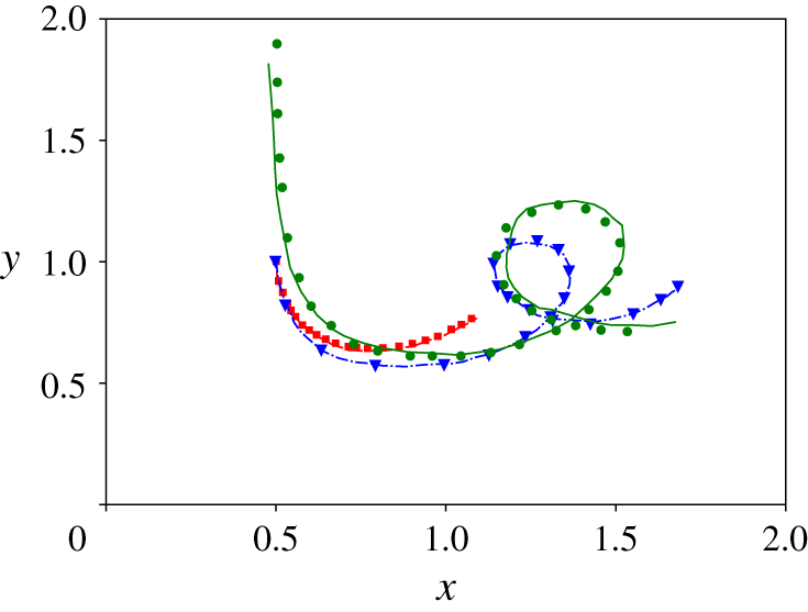
Numerical validation is carried out using comparisons of vortex trajectories against data from different simulations published by Türk et al. (Reference Türk, Coors and Jacob1999) and Zheng & Ash (Reference Zheng and Ash1996). Usually the vortex centroid  $M_{c}=(x_{c},y_{c})$ is obtained by the first moment of the normal to the plane vorticity field
 $\unicode[STIX]{x1D714}$
 $$\begin{eqnarray}x_{c}=\displaystyle {\displaystyle \frac{\displaystyle \int _{\unicode[STIX]{x1D6FA}}x\unicode[STIX]{x1D714}\,\text{d}\unicode[STIX]{x1D6FA}}{\displaystyle \int _{\unicode[STIX]{x1D6FA}}\unicode[STIX]{x1D714}\,\text{d}\unicode[STIX]{x1D6FA}}};\quad y_{c}=\displaystyle {\displaystyle \frac{\displaystyle \int _{\unicode[STIX]{x1D6FA}}y\unicode[STIX]{x1D714}\,\text{d}\unicode[STIX]{x1D6FA}}{\displaystyle \int _{\unicode[STIX]{x1D6FA}}\unicode[STIX]{x1D714}\,\text{d}\unicode[STIX]{x1D6FA}}}.\end{eqnarray}$$
However, in the present configuration,  $M_{c}$ does not match the primary vortex locus
 $M_{pv}=(x_{pv},y_{pv})$ because of the boundary layer and secondary vortices. Instead, the vortex locus
 $M_{pv}$ is taken as the barycentre of the vorticity field
 $\unicode[STIX]{x1D714}_{pv}$ given by
 $$\begin{eqnarray}\unicode[STIX]{x1D714}_{pv}(x,y)=\unicode[STIX]{x1D714}(x,y)\cdot [\unicode[STIX]{x1D714}(x,y)>0]\cdot [Q(x,y)>0],\end{eqnarray}$$
where  $[S]$ denotes the Iverson bracket of the statement
 $S$ (Iverson Reference Iverson1962) and
 $Q$ is the
 $Q$-criterion which defines a vortex as a region with a positive second invariant of
 $\unicode[STIX]{x1D735}u$ (Hunt, Wray & Moin Reference Hunt, Wray and Moin1988; Kolář Reference Kolář2007). The barycentre leading to
 $M_{pv}$ is then obtained by the same volume integration as in relation (2.2), with
 $\unicode[STIX]{x1D714}$ replaced by
 $\unicode[STIX]{x1D714}_{pv}$.
The comparison against Türk et al. (Reference Türk, Coors and Jacob1999) is conducted for  $Re_{0}=\unicode[STIX]{x1D6E4}_{0}/\unicode[STIX]{x1D708}=330$ and
 $3300$ and that against Zheng & Ash (Reference Zheng and Ash1996) for
 $Re_{0}=\unicode[STIX]{x1D6E4}_{0}/\unicode[STIX]{x1D708}=7650$ (note the use of
 $Re_{0}=2\unicode[STIX]{x03C0}Re$). The flow is initialized by a pair of Lamb–Oseen vortices localized at
 $\pm (x_{c_{0}},2x_{c_{0}})$ and
 $(\pm x_{c_{0}},3.8x_{c_{0}})$ to match the settings of Türk et al. (Reference Türk, Coors and Jacob1999) and Zheng & Ash (Reference Zheng and Ash1996), respectively. The ensemble of trajectories, shown in figure 2, provides comparisons that validate the present numerical approach.
Trajectories of the right vortex for a set of Reynolds numbers. The red, blue and green curves respectively correspond to  $Re_{0}=\unicode[STIX]{x1D6E4}_{0}/\unicode[STIX]{x1D708}=330,3300,7650$. The results obtained by Türk et al. (Reference Türk, Coors and Jacob1999) (two cases) and Zheng & Ash (Reference Zheng and Ash1996) are respectively represented with the dashed, dash-dotted and solid lines and the trajectories obtained in the simulations are marked with squares, triangles and circles.

3 Uncontrolled flow
In potential flows, vortices initially located in  $(\pm x_{c_{0}},y_{c_{0}})$ follow a hyperbolic trajectory
 $(x_{c}(t),y_{c}(t))$ described by
 $$\begin{eqnarray}\frac{1}{x_{c}^{2}(t)}+\frac{1}{y_{c}^{2}(t)}=\frac{1}{x_{c_{0}}^{2}}+\frac{1}{y_{c_{0}}^{2}}.\end{eqnarray}$$
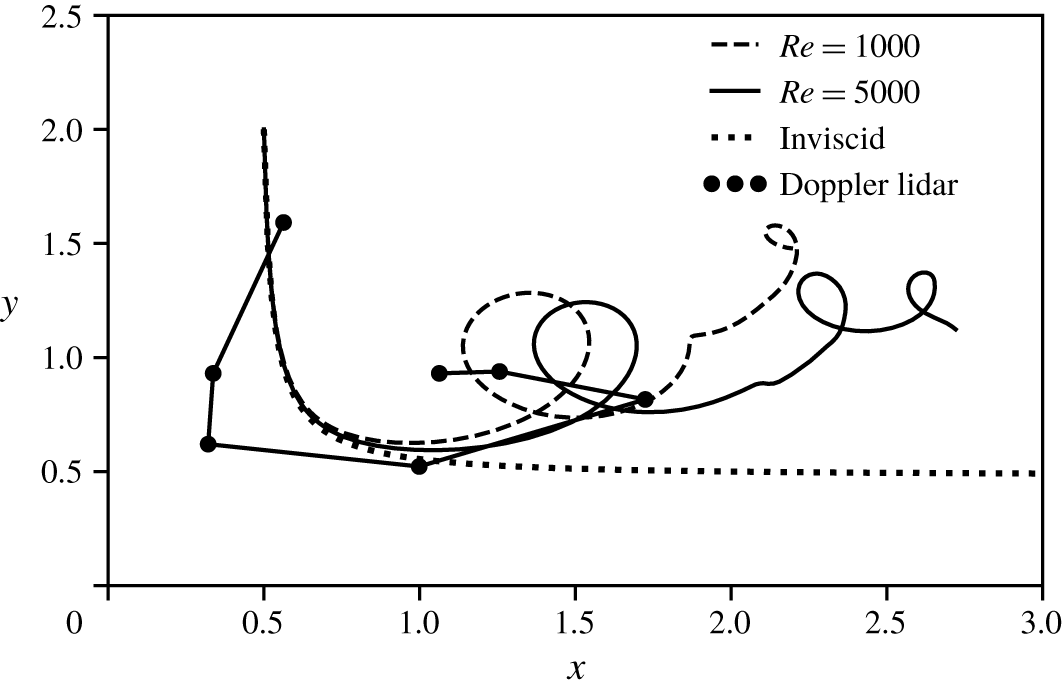
With viscosity, as seen previously in figure 2 and now in figure 3 which plots the vortex trajectories for  $Re=500$ and 1000, the dynamics is modified when the vortices near the ground. This so-called rebound results in an oscillation of the altitude of the vortex and a reduction of its sideward motion. It is noteworthy that such an observation is coherent with practical, high Reynolds number cases of aircraft wake vortices impacting ground, as is shown by the lidar (light detection and ranging) measurements also plotted in figure 3. The data come from a set of Doppler lidar measurements performed at Toulouse-Blagnac airport (Hallermeyer Reference Hallermeyer2017). From the simulated data it can be remarked that with a larger Reynolds number the vortex follows the inviscid path up to a larger distance. Rebound yet remains practically unchanged, given that both the current simulations and the real life lidar measurements show identical overall kinematics.
Trajectories of the right vortex for  $Re=1000$ (dashed line), for
 $Re=5000$ (solid line) and inviscid flow (dotted line). Simulation time is
 $t=15$. Circle markers correspond to Doppler lidar measurements achieved at Toulouse-Blagnac airport (European Commission 2015; Hallermeyer Reference Hallermeyer2017) during
 $50$ s (in this case
 $b\simeq 40~\text{m}$ and circulation is
 $\unicode[STIX]{x1D6E4}_{0}\simeq 500~\text{m}^{2}~\text{s}^{-1}$). Note the existence of an average cross-wind (
 $u_{crosswind}\sim -1~\text{m}~\text{s}^{-1}$) in the lidar case, not taken into account in the simulated data.

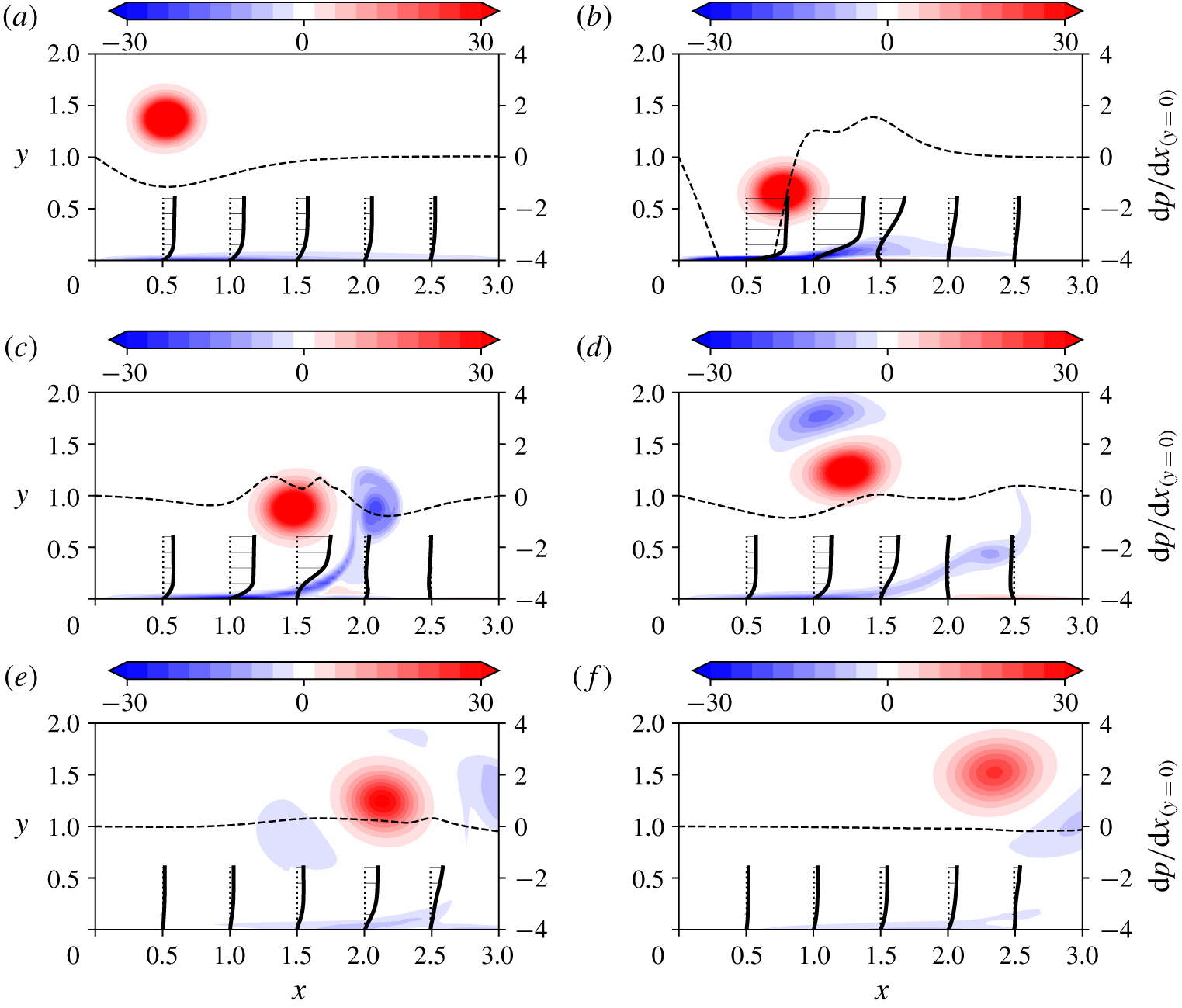
Rebound is illustrated in figure 4 with plots of the vorticity field at various instants of the vortex evolution. The figure also features a set of velocity profiles in the near wall region and the wall-wise pressure gradient. The velocity profiles show the flow at the wall that is induced by the momentum brought by the vortices. As initially described by Harvey & Perry (Reference Harvey and Perry1971) and due to the large Reynolds number, this subsequently forms a boundary layer. The vortex also imposes a positive pressure gradient at its sides because of the low pressure present in its core. As a consequence of this (adverse) pressure gradient, the boundary layer separates. This occurs when the vortex gets closer to the ground (figure 4b). The separated flow then rolls into opposite sign vorticity, soon embarked around the primary vortex (c). Additional detachments of the separated boundary layer later form other vortices, which themselves induce an opposite boundary layer flow (d).
Uncontrolled vorticity field computed for  $Re=1000$ at
 $t=0.25,2.5,3.75,5,10,15$. Thick lines represent boundary layer profiles are given at locations
 $x=0.5,1,1.5,2.0,2.5$. Dashed lines represent the pressure gradient along the wall (at
 $y=0$). (a) Descending vortex
 $t=1.25$. (b) Boundary layer and detachment of a secondary vortex
 $t=2.5$. (c) Rebound of the vortex
 $t=3.75$. (d) Entrainment of the secondary vortex
 $t=5$. (e) Entrainment of the secondary vortex
 $t=10$. (f) Entrainment of the secondary vortex
 $t=15$.

The question of how the vortex circulation evolves in this context can be analysed using the circulation of the right part of the flow  $\unicode[STIX]{x1D6E4}_{tot}=\int _{\unicode[STIX]{x1D6FA}}\unicode[STIX]{x1D714}\,\text{d}\unicode[STIX]{x1D6FA}$, whose evolution is to be inferred from the equation of the vorticity
 $\unicode[STIX]{x1D714}$
 $$\begin{eqnarray}\frac{\text{d}\unicode[STIX]{x1D6E4}_{tot}}{\text{d}t}=\frac{1}{Re}\int _{\unicode[STIX]{x2202}\unicode[STIX]{x1D6FA}}\unicode[STIX]{x1D735}\unicode[STIX]{x1D714}\boldsymbol{\cdot }\boldsymbol{n}\unicode[STIX]{x2202}\unicode[STIX]{x1D6FA}=-\frac{1}{Re}\left(\int _{\unicode[STIX]{x2202}\unicode[STIX]{x1D6FA}_{1}}\frac{\unicode[STIX]{x2202}\unicode[STIX]{x1D714}}{\unicode[STIX]{x2202}y}\,\text{d}x+\int _{\unicode[STIX]{x2202}\unicode[STIX]{x1D6FA}_{4}}\frac{\unicode[STIX]{x2202}\unicode[STIX]{x1D714}}{\unicode[STIX]{x2202}x}\,\text{d}y\right).\end{eqnarray}$$
Since  $\unicode[STIX]{x2202}\unicode[STIX]{x1D714}/\unicode[STIX]{x2202}x>0$ at
 $\unicode[STIX]{x2202}\unicode[STIX]{x1D6FA}_{4}$, the left boundary, and
 $\unicode[STIX]{x2202}\unicode[STIX]{x1D714}/\unicode[STIX]{x2202}y>0$ at
 $\unicode[STIX]{x2202}\unicode[STIX]{x1D6FA}_{1}$, the bottom boundary, total circulation is expected to decrease. Physically the second and first terms on the right-hand side relate to friction with the left vortex and ground, respectively. It is important to mention that total circulation
 $\unicode[STIX]{x1D6E4}_{tot}$ is not equal to
 $\unicode[STIX]{x1D6E4}_{0}$ initially because of the presence of the boundary layer, which features negative vorticity.
To characterize the vortex circulation,  $\unicode[STIX]{x1D6E4}_{pv}$ is introduced, which is defined as
 $$\begin{eqnarray}\unicode[STIX]{x1D6E4}_{pv}=\int _{\unicode[STIX]{x1D6FA}_{pv}}\unicode[STIX]{x1D714}\,\text{d}\unicode[STIX]{x1D6FA}_{pv}.\end{eqnarray}$$
The configuration imposes  $\unicode[STIX]{x1D6E4}_{pv}=\unicode[STIX]{x1D6E4}_{0}$ initially. The zone
 $\unicode[STIX]{x1D6FA}_{pv}$ defines the spatial extent of the primary vortex. Here, to discriminate it from the several vortical zones featured by the flow,
 $\unicode[STIX]{x1D6FA}_{pv}$ is defined as the zone of positive vorticity about the primary vortex locus
 $M_{pv}=(x_{pv},y_{pv})$. Note that the simple integration of
 $\unicode[STIX]{x1D714}_{pv}$ over the half-domain
 $\unicode[STIX]{x1D6FA}$, as used to define
 $M_{pv}$ in (2.3), does not yield the vortex circulation as desired, as, due to the
 $Q$-criterion constraint, it misses some part of the vortical area associated with the vortex. The zone
 $\unicode[STIX]{x1D6FA}_{pv}$ cannot be easily described and therefore a specific procedure is employed to automatically track its shape in the snapshots of the flow. The first step is to locate the primary vortex centre using procedure (2.3). Once the vortex centre is known, the method consists in using a cylindrical coordinate system about
 $M_{pv}$ and to locate at all azimuthal positions
 $\unicode[STIX]{x1D703}$ the radial extent
 $R$ where
 $\unicode[STIX]{x1D714}_{pv}(R,\unicode[STIX]{x1D703})=0$. In practice, an ensemble of
 $N_{\unicode[STIX]{x1D703}}=128$ azimuthal positions
 $\unicode[STIX]{x1D703}_{i}$ is considered, and the radial direction is discretized into
 $R_{i}$ with a spacing of
 $\unicode[STIX]{x1D6FF}_{r}=0.01$. The ensemble of
 $(\unicode[STIX]{x1D703}_{i},R_{i})$ forms a polygonal area that is taken as
 $\unicode[STIX]{x1D6FA}_{pv}$.
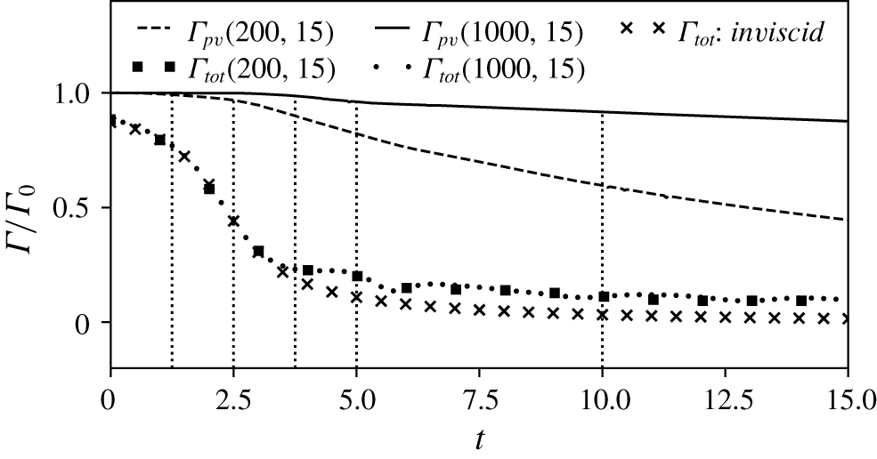
Evolution of  $\unicode[STIX]{x1D6E4}_{pv}$ and
 $\unicode[STIX]{x1D6E4}_{tot}$ at
 $Re=200,1000$ and
 $T=15$ for the uncontrolled case. Vertical dotted lines correspond to times
 $t=1.25,2.5,3.75,5,10$ referring to figure 4.

Figure 5 shows the evolution of  $\unicode[STIX]{x1D6E4}_{tot}$ and
 $\unicode[STIX]{x1D6E4}_{pv}$ as a function of time for the two Reynolds numbers
 $Re=200$ and 1000. Total circulation
 $\unicode[STIX]{x1D6E4}_{tot}$ is seen to decrease significantly up to
 $t=4$ and to level off after that. This can be analysed in the light of figure 4, which corresponds to the case
 $Re=1000$. Indeed the development of the boundary layer, its separation and the formation of the secondary vortex (see figure 4a–c) explain the initial strong decrease of
 $\unicode[STIX]{x1D6E4}_{tot}$ in figure 5 while the mild decrease of total circulation after
 $t=4$ stems from the end of these processes and corresponds to the slow viscous interaction between the different vorticity zones.
It is observed that the evolution of  $\unicode[STIX]{x1D6E4}_{tot}$ hardly changes between
 $Re=200$ and 1000, suggesting a weak Reynolds number dependency of this quantity. The formulation of circulation written below
 $$\begin{eqnarray}\unicode[STIX]{x1D6E4}_{tot}=\oint _{\unicode[STIX]{x2202}\unicode[STIX]{x1D6FA}}\boldsymbol{u}\boldsymbol{\cdot }\text{d}\boldsymbol{l},\end{eqnarray}$$
can help understand why this is so. In (3.4)  $\text{d}\boldsymbol{l}$ is the tangent vector along the closed contour
 $\unicode[STIX]{x2202}\unicode[STIX]{x1D6FA}$. In the no-slip case, the contour integration reduces to the symmetry boundary
 $\unicode[STIX]{x2202}\unicode[STIX]{x1D6FA}_{4}$. Indeed, the velocities at the top and right boundaries are very small and their contribution can thus be neglected. Equation (3.4) can hence be rewritten as
 $$\begin{eqnarray}\unicode[STIX]{x1D6E4}_{tot}=-\int _{\unicode[STIX]{x2202}\unicode[STIX]{x1D6FA}_{4}}v(0,y)\,\text{d}y,\end{eqnarray}$$
where  $\unicode[STIX]{x2202}\unicode[STIX]{x1D6FA}_{4}$ is oriented downward. The vertical velocity at the symmetry plane
 $v(0,y)$ essentially evolves as a function of the lateral distance of the vortex and one expects little influence of the no-slip boundary condition applied at the ground. As a check, we introduce
 $\unicode[STIX]{x1D6E4}_{inv}=-\int _{\unicode[STIX]{x2202}\unicode[STIX]{x1D6FA}_{4}}v_{inv}(0,y)\,\text{d}y$, the contribution of the left symmetry frontier to the total circulation in the inviscid case. The velocity
 $v_{inv}$ results from the Biot–Savart law applied to the point vortex along the hyperbolic trajectory and its images. This circulation can be calculated following
 $$\begin{eqnarray}\unicode[STIX]{x1D6E4}_{inv}=\int _{\unicode[STIX]{x2202}\unicode[STIX]{x1D6FA}_{4}}{\displaystyle \frac{\unicode[STIX]{x1D6E4}_{0}}{2\unicode[STIX]{x03C0}}}\left\{{\displaystyle \frac{2x_{c}}{\sqrt{x_{c}^{2}+(y-y_{c})^{2}}}}-{\displaystyle \frac{2x_{c}}{\sqrt{x_{c}^{2}+(y+y_{c})^{2}}}}\right\}\,\text{d}y.\end{eqnarray}$$
Crossed markers in figure 5 show the time evolution of total circulation using (3.6). The evolution of  $\unicode[STIX]{x1D6E4}_{inv}$ follows closely that of
 $\unicode[STIX]{x1D6E4}_{tot}$ provided by (3.2) up to
 $t=3$. Departure from the inviscid evolution appears afterwards, indicating the impact of no slip at the ground on the lateral position of the vortex. However the difference between
 $\unicode[STIX]{x1D6E4}_{inv}$ and
 $\unicode[STIX]{x1D6E4}_{tot}$ remains small, which concludes on the weak influence of Reynolds number on
 $\unicode[STIX]{x1D6E4}_{tot}$.
The circulation of the primary vortex  $\unicode[STIX]{x1D6E4}_{pv}$ shows a different evolution than
 $\unicode[STIX]{x1D6E4}_{tot}$, with three distinct phases and a net effect of Reynolds number. The first phase, that corresponds to the initial descent of the vortices, up to
 $t=2.5$, preserves circulation, i.e.
 $\unicode[STIX]{x1D6E4}_{pv}\simeq \unicode[STIX]{x1D6E4}_{0}$. The second phase, up to
 $t=5$, features a sudden drop of circulation and coincides with the rebound of the vortex. In this step the vortex experiences strong friction at the wall because
 $\unicode[STIX]{x1D735}\unicode[STIX]{x1D714}\boldsymbol{\cdot }\boldsymbol{n}$ is increased by the presence of opposite sign vorticity at the wall (boundary layer). The decay rate then slightly levels off, corresponding to the third phase of evolution. Vortex decay in the two last phases shows a clear dependence upon the Reynolds number. The start of the third phase (
 $t\geqslant 5$) corresponds to the slow decay phase of the total circulation
 $\unicode[STIX]{x1D6E4}_{tot}$, and to the quasi-disappearance of the pressure gradient at the wall, which goes along with the quasi-suppression of the boundary layer, see figure 4. The vortex system altitude is now large due to the previous rebound and the friction at the wall is not as significant.
4 Optimal control approach
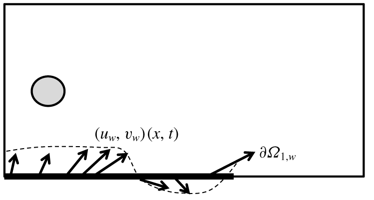
We consider the effect of either blowing or suction applied at the ground to counteract the stagnation of the vortex system and promote increased lateral displacement. Practically, a modification of the boundary condition at  $\unicode[STIX]{x2202}\unicode[STIX]{x1D6FA}_{1}$ in (2.1) is applied with
 $\boldsymbol{u}_{\unicode[STIX]{x2202}\unicode[STIX]{x1D6FA}_{1}}=\boldsymbol{u}_{\boldsymbol{w}}(x,t)$ where
 $\boldsymbol{u}_{\boldsymbol{w}}(x,t)$ is free to vary in intensity and orientation. The control is restricted to a zone of finite extent
 $\unicode[STIX]{x2202}\unicode[STIX]{x1D6FA}_{1,w}=\{0\leqslant x\leqslant 10\}$. Figure 6 provides a schematic of the control set-up.
Schematic of the control scheme applied along the portion  $\unicode[STIX]{x2202}\unicode[STIX]{x1D6FA}_{1,w}$ of the wall.
 $u_{w}$ and
 $v_{w}$ denote the flow velocity imposed at the wall.

The optimal control strategy requires an appropriate objective function  ${\mathcal{J}}$ to optimize
 $\boldsymbol{u}_{\boldsymbol{w}}$ and maximize the lateral position of the vortex system at a given horizon time
 $T$. A choice could have been the first moment of vorticity
 $\int _{\unicode[STIX]{x1D6FA}}x\unicode[STIX]{x1D714}\,\text{d}\unicode[STIX]{x1D6FA}$ as it evaluates, once divided by
 $\unicode[STIX]{x1D6E4}_{tot}$ (see (2.2)), the horizontal component of the barycentre of vorticity.
However, because of the different vorticity areas, which yield opposite signs, this optimization would lead to maximizing the lateral position of the positive vorticity (primary vortex) and minimizing that of the negative vorticity (separated boundary layer). Therefore, the maximization of the lateral position of the vortex seems not to be guaranteed. A way to shape the objective function to our goal is to consider instead the square of vorticity  $\unicode[STIX]{x1D714}^{2}$. The benefit is that it mechanically embarks the vorticity of the primary vortex and the opposite vorticity coming from the separated boundary layer alike.
The implementation hence proceeds from an evaluation of the horizontal position of the vortex based on the horizontal component of the barycentre of vorticity squared, that is
 $$\begin{eqnarray}{\mathcal{J}}(\boldsymbol{u};\boldsymbol{u}_{\boldsymbol{w}};T,l)={\mathcal{J}}_{1}(\boldsymbol{u};\boldsymbol{u}_{\boldsymbol{w}};T,l)-l{\mathcal{J}}_{2}(\boldsymbol{u}_{\boldsymbol{w}};T,l),\end{eqnarray}$$
with
 $$\begin{eqnarray}{\mathcal{J}}_{1}(\boldsymbol{u};\boldsymbol{u}_{\boldsymbol{w}};T,l)=\displaystyle {\displaystyle \frac{\displaystyle \int _{\unicode[STIX]{x1D6FA}}x\unicode[STIX]{x1D714}^{2}(T)\,\text{d}\unicode[STIX]{x1D6FA}}{\displaystyle \int _{\unicode[STIX]{x1D6FA}}\unicode[STIX]{x1D714}^{2}(T)\,\text{d}\unicode[STIX]{x1D6FA}}},\end{eqnarray}$$
and
 $$\begin{eqnarray}\displaystyle {\mathcal{J}}_{2}(\boldsymbol{u}_{\boldsymbol{w}};T,l)=\displaystyle {\displaystyle \frac{1}{2}}\int _{0}^{T}\int _{\unicode[STIX]{x2202}\unicode[STIX]{x1D6FA}_{1}}\boldsymbol{u}_{\boldsymbol{w}}^{2}\,\text{d}x\,\text{d}t.\end{eqnarray}$$
The term  ${\mathcal{J}}_{2}$ (spatio-temporal norm of the control) penalizes
 ${\mathcal{J}}_{1}$ by acting as a cost function for control. The mathematical parameter
 $l>0$ (which holds no physical interpretation) prevents
 $\boldsymbol{u}_{\boldsymbol{w}}$ from reaching an unphysically large amplitude and increases the convergence of the optimization algorithm. As such, it favours the existence and unicity of a solution as well as eases convergence of the optimization loops. The case
 $l\rightarrow \infty$ amounts to the uncontrolled case i.e.
 ${\mathcal{J}}_{m}(\cdot ,\infty )={\mathcal{J}}_{1}(\cdot ,\infty )$ since
 $\lim _{l\rightarrow \infty }{\mathcal{J}}_{2}=0$ (a validation is provided further down, see § 5.1).
The maximum  ${\mathcal{J}}_{m}(T,l)$ of
 ${\mathcal{J}}$ in the space of
 $\boldsymbol{u}_{w}$ for a given
 $T$ and
 $l$ is found using the Lagrange multiplier method in which the constrained optimization problem is transformed into an unconstrained one. To this end, the cost functional and the constraints are assembled into the Lagrangian function
 ${\mathcal{L}}$, in the form
 $$\begin{eqnarray}\displaystyle \displaystyle {\mathcal{L}}(\boldsymbol{u},\boldsymbol{u}^{+},p,p^{+},\boldsymbol{u}_{\boldsymbol{w}},\boldsymbol{u}_{\boldsymbol{w}}^{+}) & = & \displaystyle {\mathcal{J}}(\boldsymbol{u}_{\boldsymbol{w}})-\left[\unicode[STIX]{x2202}_{t}\boldsymbol{u}+(\boldsymbol{u}\boldsymbol{\cdot }\unicode[STIX]{x1D735})\boldsymbol{u}+\unicode[STIX]{x1D735}p-{\displaystyle \frac{1}{Re}}\unicode[STIX]{x1D6FB}^{2}\boldsymbol{u},\boldsymbol{u}^{+}\right]\nonumber\\ \displaystyle & & \displaystyle -\,[\unicode[STIX]{x1D735}\boldsymbol{\cdot }~\boldsymbol{u},p^{+}]-(\boldsymbol{u}-\boldsymbol{u}_{\boldsymbol{w}},\boldsymbol{u}_{\boldsymbol{w}}^{+}),\end{eqnarray}$$
where  $[\cdot ,\cdot ]$ and
 $(\cdot ,\cdot )$, denote the following inner products
 $$\begin{eqnarray}\left.\begin{array}{@{}c@{}}[\boldsymbol{a}(\boldsymbol{x},t),\boldsymbol{b}(\boldsymbol{x},t)]=\displaystyle \int _{0}^{T}\int _{\unicode[STIX]{x1D6FA}}\boldsymbol{a}(\boldsymbol{x},t)\boldsymbol{\cdot }\boldsymbol{b}(\boldsymbol{x},t)\,\text{d}\unicode[STIX]{x1D6FA}\text{d}t,\\[12.0pt] (\boldsymbol{c}(x),\boldsymbol{d}(x))=\displaystyle \int _{\unicode[STIX]{x2202}\unicode[STIX]{x1D6FA}_{1}}\boldsymbol{c}(x)\boldsymbol{\cdot }\boldsymbol{d}(x)\,\text{d}x,\end{array}\right\}\end{eqnarray}$$
and  $\boldsymbol{a},\boldsymbol{b}$ are functions of space and time and
 $\boldsymbol{c},\boldsymbol{d}$ are functions of space alone.
The Lagrangian function  ${\mathcal{L}}$ depends on the direct
 $(\boldsymbol{u},p,\boldsymbol{u}_{\boldsymbol{w}})$ variables and Lagrange multipliers
 $(\boldsymbol{u}^{+},p^{+},\boldsymbol{u}_{\boldsymbol{w}}^{+})$, also known as adjoint variables. The optimal control is found by cancelling the first variation of the Lagrangian with respect to its variables. For a complete derivations of these equations the reader is referred to Choi et al. (Reference Choi, Hinze and Kunisch1999). Here, only the most important relations are provided. The first variation of
 ${\mathcal{L}}$ with respect to the adjoint variables yields the equations of the constraints and the first variation with respect to the direct variables provides a set of equations for the adjoint variables,
 $$\begin{eqnarray}\left.\begin{array}{@{}l@{}}\unicode[STIX]{x1D735}\boldsymbol{\cdot }~\boldsymbol{u}^{+}=0,\\ -\unicode[STIX]{x2202}_{t}\boldsymbol{u}^{+}-(\boldsymbol{u}\boldsymbol{\cdot }\unicode[STIX]{x1D735})\boldsymbol{u}^{+}+(\unicode[STIX]{x1D735}\boldsymbol{u})^{\intercal }\boldsymbol{u}^{+}=-\unicode[STIX]{x1D735}p^{+}+{\displaystyle \frac{1}{Re}}\unicode[STIX]{x1D6FB}^{2}\boldsymbol{u}^{+},\end{array}\right\}\end{eqnarray}$$
where  $^{\intercal }$ denotes the transpose operator. The minus sign in front of the time partial derivative can be interpreted as a change of variable
 $t\longrightarrow T-t$. As a consequence, the adjoint equation is solved backward in time from
 $t=T$ to
 $t=0$. By matching terms of the integration by part of the partial time derivative, one obtains the following compatibility equation (which is derived in appendix A) for
 $t=T$
 $$\begin{eqnarray}\boldsymbol{u}^{+}(\boldsymbol{x},T)={\displaystyle \frac{2}{I_{0}(T)}}(x\unicode[STIX]{x1D735}\times \unicode[STIX]{x1D714}(T)\boldsymbol{e}_{z}+\unicode[STIX]{x1D735}x\times \unicode[STIX]{x1D714}(T)\boldsymbol{e}_{z})-{\displaystyle \frac{2I_{1}(T)}{I_{0}(T)^{2}}}(\unicode[STIX]{x1D735}\times \unicode[STIX]{x1D714}(T)\boldsymbol{e}_{z}),\end{eqnarray}$$
where
 $$\begin{eqnarray}\displaystyle I_{0}(t)=\int _{\unicode[STIX]{x1D6FA}}\unicode[STIX]{x1D714}^{2}(t)\,\text{d}\unicode[STIX]{x1D6FA},\end{eqnarray}$$
and
 $$\begin{eqnarray}\displaystyle I_{1}(t)=\int _{\unicode[STIX]{x1D6FA}}x\unicode[STIX]{x1D714}^{2}(t)\,\text{d}\unicode[STIX]{x1D6FA}.\end{eqnarray}$$
Relation (4.7) initializes the adjoint variable  $\boldsymbol{u}^{+}(\boldsymbol{x},T)$. The gradient of the Lagrangian with respect to
 $\boldsymbol{u}_{\boldsymbol{w}}$
 $$\begin{eqnarray}\unicode[STIX]{x1D735}_{\boldsymbol{u}_{\boldsymbol{w}}}{\mathcal{L}}=-l\boldsymbol{u}_{\boldsymbol{w}}+\boldsymbol{u}_{\boldsymbol{w}}^{+}=-l\boldsymbol{u}_{\boldsymbol{ w}}+\left(p^{+}(x,y=0,t)-{\displaystyle \frac{1}{Re}}{\displaystyle \frac{\unicode[STIX]{x2202}\boldsymbol{u}^{+}}{\unicode[STIX]{x2202}y}}(x,y=0,t)\right)\boldsymbol{e}_{\boldsymbol{y}},\end{eqnarray}$$
eventually provides the direction to follow in order to update the control variable.
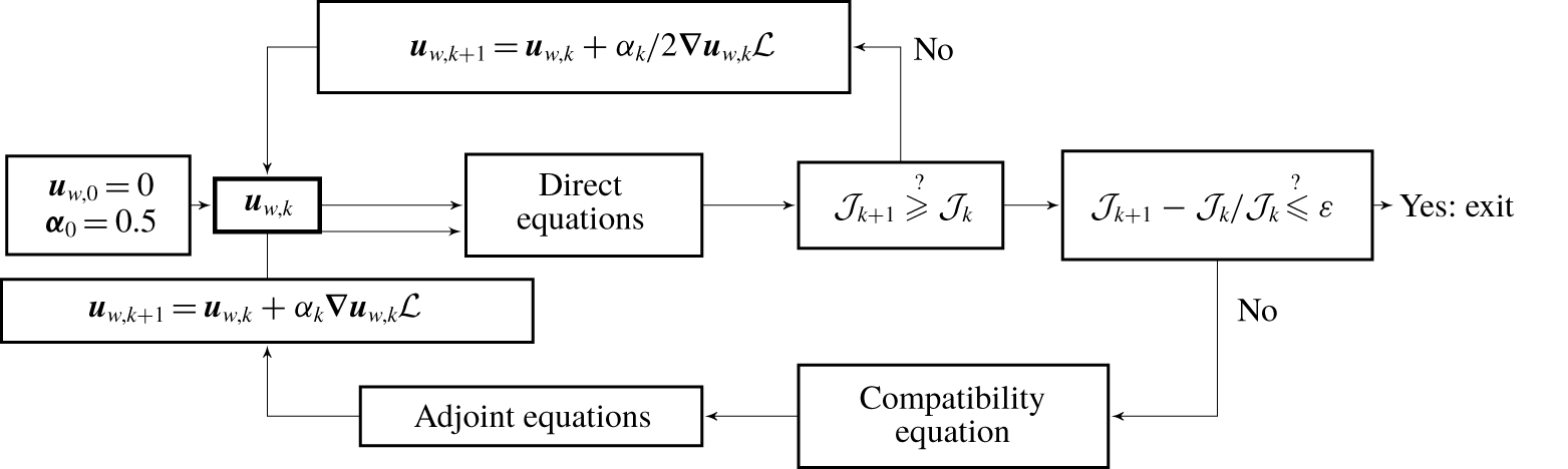
This optimal system is based on a set of nonlinear partial differential equations. While this nonlinearity could lead to difficulties in converging an optimal solution, in the present case the dynamics of the vortex to be controlled follows a deterministic evolution, so that similarly to Önder & Meyers (Reference Önder and Meyers2016), a steepest descent algorithm with a generic backtracking line search is successfully used in order to perform the optimization. The whole procedure is sketched in figure 7. Starting from an initial  $\boldsymbol{u}_{w,0}=0$, the algorithm follows two loops. The main loop goes towards the optimal velocity at the wall by computing the gradient and updating
 $\boldsymbol{u}_{w}$ with a factor
 $\unicode[STIX]{x1D6FC}_{k}$ of the gradient. The second loop concerns the line search to adapt the value of
 $\unicode[STIX]{x1D6FC}_{k}$ when the chosen value does not optimize. The starting value is 0.5. Whenever the chosen value does not lead to optimization,
 $\unicode[STIX]{x1D6FC}_{k}$ is halved and the direct simulation is repeated until optimization is achieved. The iterative algorithm is eventually stopped when
 $({\mathcal{J}}_{k+1}-{\mathcal{J}}_{k})/{\mathcal{J}}_{k}\leqslant \unicode[STIX]{x1D700}=10^{-4}$.
Sketch of the optimization algorithm. The line search parameter is  $\unicode[STIX]{x1D6FC}_{k}$.

In the current algorithm the cost of storing the control variable when integrating the adjoint is decreased by using linear interpolation over uniform time intervals  $[t_{i},t_{i+1}]$ of the horizon time
 $T$
 $$\begin{eqnarray}\boldsymbol{u}_{\boldsymbol{w}}(t_{k})=\unicode[STIX]{x1D6FD}_{k}\boldsymbol{u}_{\boldsymbol{w}}(t_{i})+(1-\unicode[STIX]{x1D6FD}_{k})\boldsymbol{u}_{\boldsymbol{w}}(t_{i+1}),\end{eqnarray}$$
where  $\unicode[STIX]{x1D6FD}_{k}=(t_{i+1}-t_{k})/\unicode[STIX]{x0394}t$ and
 $\unicode[STIX]{x1D6FF}t_{i}=t_{i+1}-t_{i}$ is chosen such that
 $\unicode[STIX]{x1D6FF}t_{i}\leqslant 5\,\%$. The convergence of the results is provided in appendix B.1 and convergence in
 $\unicode[STIX]{x1D6FF}t_{i}$ is shown in appendix B.2.
5 Controlled flow
5.1 Optimal parameters
Optimizations have been carried out for  $T\in [2,10]$ and
 $l\in [1,100]$, and Reynolds numbers of 200 and 1000.
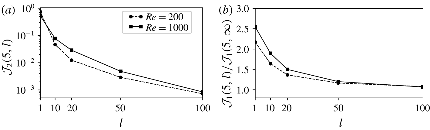
(a) Evolution of the cost of control  ${\mathcal{J}}_{2}$ as a function of
 $l$ for Reynolds numbers 200 and 1000,
 $T=5$, showing that the optimal control amounts to the uncontrolled case for increasing values of
 $l$. (b) Ratio
 ${\mathcal{J}}_{1}(5,l)/{\mathcal{J}}_{1}(5,\infty )$ as a function of the penalization coefficient for computations carried at
 $Re=200$ (dashed line and crosses) and
 $Re=1000$ (solid line and squared markers) for
 $T=5$.

In figure 8(a) the cost of control  ${\mathcal{J}}_{2}$ is plotted as a function of
 $l$. It shows, as expected, that growing
 $l$ returns to the uncontrolled case
 ${\mathcal{J}}_{2}\rightarrow 0$. Low values of
 $l$ have been tested and have shown that when
 $l<1$ the optimization breaks down: the intensity of
 $\boldsymbol{u}_{w}$ becomes too high for the capability of the mesh and time step that are used (which correspond to the initial simulation of the uncontrolled case). Figure 8(b) shows the optimized vortex barycentre
 ${\mathcal{J}}_{1}$ normalized upon its value for infinite
 $l$ (no control) as a function of
 $l$ for
 $Re=200$ and 1000. It shows that the gain increases as
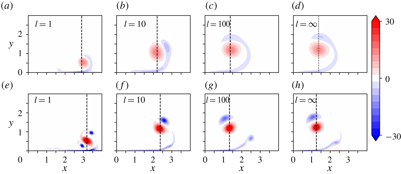
 $l$ is lowered, reaching a maximum of 1.5 and 2 for
 $l=1$ at the two Reynolds numbers, respectively. Increasing Reynolds number yields a favourable effect for augmenting control capacity. Plots of the vorticity field at final time
 $t=T=5$ for selected values of
 $l\in [1,\infty ]$ and the two values of Reynolds number are displayed in figure 9. They show the effect of control on the separation pattern and timing of the boundary layer and the intensity, location and number of the secondary vortices that rotate around the primary one.
Vorticity field at horizon time  $T=5$ for
 $Re=200$ (a–d) and 1000 (e–h) for increasing
 $l$. Dashed lines show the locations of the vorticity-squared barycentres,
 ${\mathcal{J}}_{1}(5,l)$.

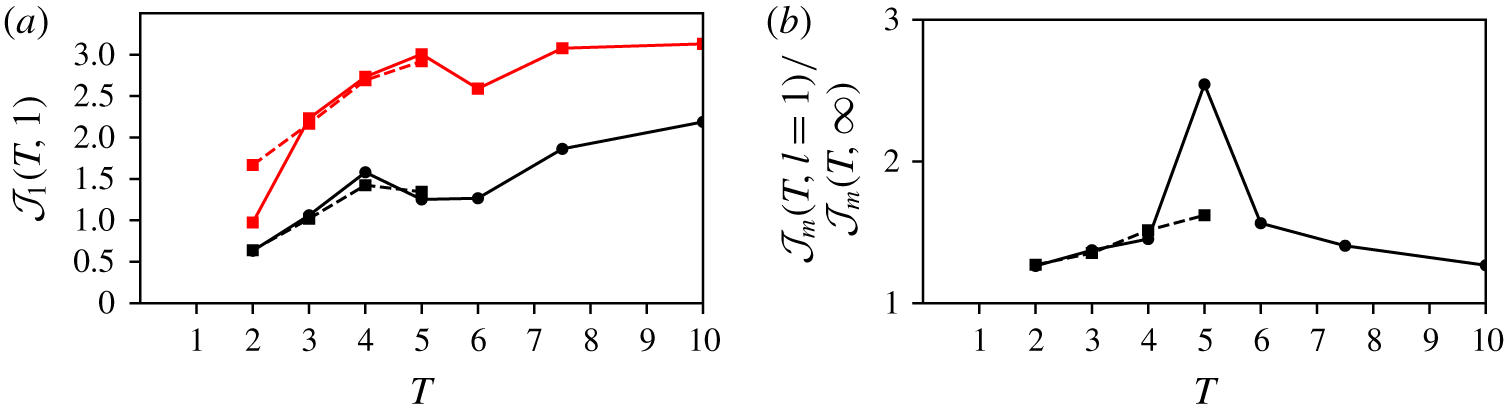
The effect of horizon time  $T$ is shown in figure 10 for
 $Re=200$ and
 $Re=1000$ at
 $l=1$, the best value within the range under consideration. Figure 10(a) plots the absolute position of the vortex
 ${\mathcal{J}}_{1}(T,l)$ for the uncontrolled and controlled cases. The increase in lateral distance provided by control is apparent from the offset between the two curves. Above
 $T=5$, the lateral position of the vortex shows a limit at approximately
 $x=3$ and no decisive increase beyond that time. Since
 $l=1$ provides the strongest control effect, this shows that optimization at a larger time is not required:
 $T=5$ appears to be quasi-optimal for the present parameter space.
For  $Re=200$, it is found that optimization cannot be carried out beyond
 $T=5$. Indeed, the routine produces irregular vorticity at the end of the domain
 $\unicode[STIX]{x2202}\unicode[STIX]{x1D6FA}_{1,w}$, which is attributed to the finite length of the control area at the ground. Coincidentally, the vortex is also sucked by the control at the wall and disappears. Calculations beyond
 $T=5$ are not conducted for
 $Re=200$.
Figure 10(b) shows the amplification of the full functional  ${\mathcal{J}}_{m}$ between the controlled and uncontrolled cases. It shows that the optimal for
 $T=5$ is also the time for which the dynamics can be optimally balanced between the possibility of increased lateral displacement and cost of control. This shows that an optimal time exists over the parameter range investigated here, at approximately 5.
Effect of horizon time. (a) Evolution of the vortex position  ${\mathcal{J}}_{1}(T,l)$ for
 $Re=200,1000$, respectively in dashed and dotted lines, for the uncontrolled case
 $l=\infty$ (black) and for
 $l=1$ (red). (b) Evolution of the ratio
 ${\mathcal{J}}_{m}(T,1)/{\mathcal{J}}_{m}(T,\infty )$, computed for
 $Re=200$ (dashed line),
 $Re=1000$ (solid lines) and
 $l=1$. For this value of
 $l$ and
 $Re=200$, increasing the horizon time, beyond
 $T\geqslant 5$, leads to the complete absorption of the primary vortex. No data are consequently available for larger time.

5.2 Physical mechanisms
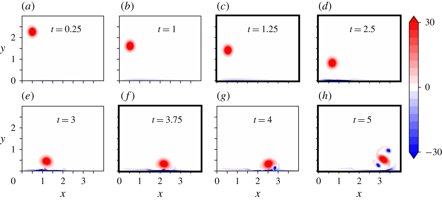
The physics behind the action of control is now analysed. The time sequence displayed in figure 11, which is obtained for  $T=5$ and corresponds to the same Reynolds number (
 $Re=1000$) as the uncontrolled one shown in figure 4, is used in preamble. Some of the time indices used in figure 4 are also repeated in figure 11, to ease the comparison. The main effect of control which can be seen in this time sequence is the delay in boundary layer separation, which is only apparent near the final time
 $t>4$, while in the uncontrolled case (figure 4) it is already effective at
 $t=2.5$. The doubling of the lateral distance, presented in the previous section, is also directly visible here, changing from
 $x\simeq 1.2$ (see figure 4d) to
 $x\simeq 3$ when control is active. Interestingly, the vortex kinematics under the effect of control bears a strong similarity to the vortex evolution obtained with the
 $v$-control scheme developed by Choi et al. (Reference Choi, Moin and Kim1994) (figure 22b).
Vorticity field in the controlled case, computed for  $(Re,T,l)=(1000,5,10)$, showing the sequence up to the optimization time
 $t=5$. Thicker borders refer to the times used in figure 4 showing the uncontrolled case at the same Reynolds number, with the same iso-contours. Note however the different spatial extensions of the plots.

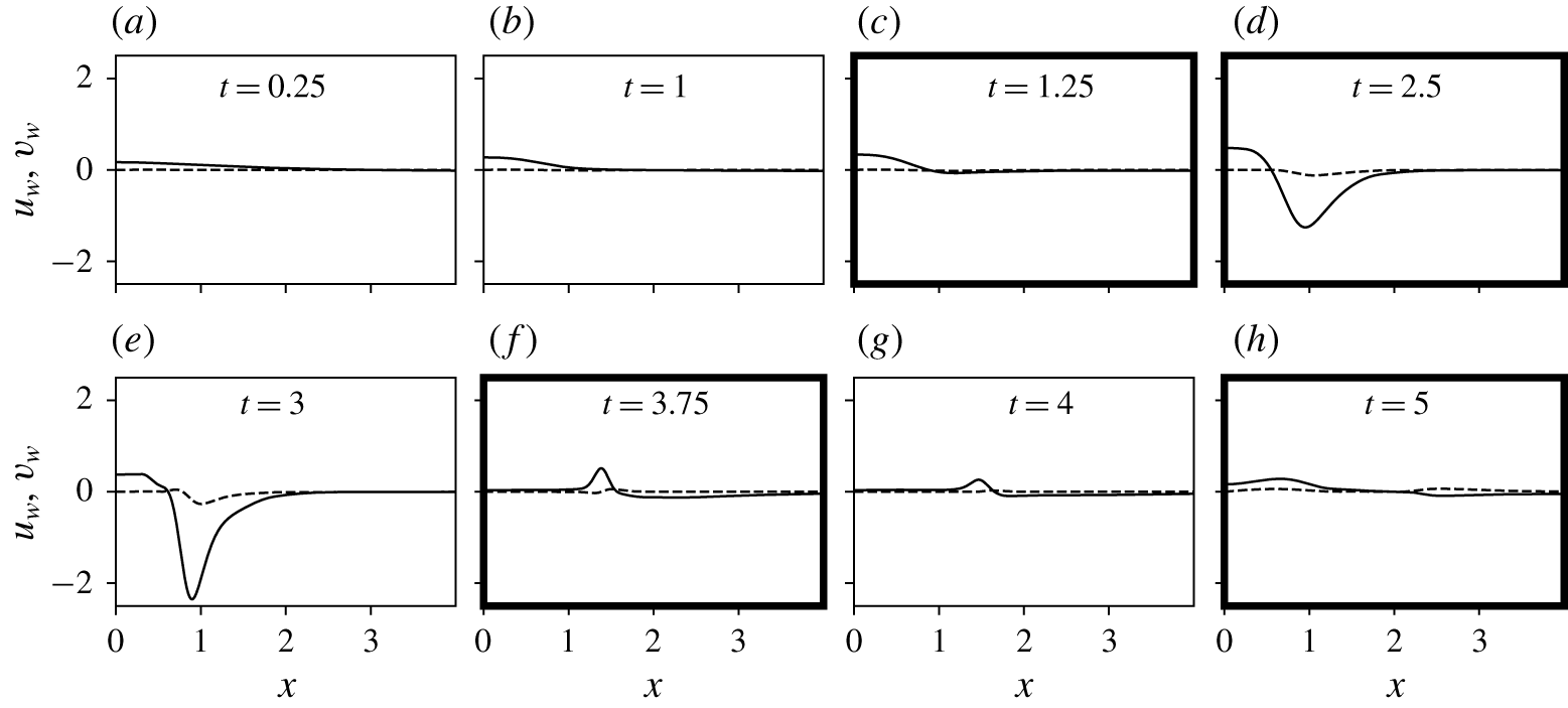
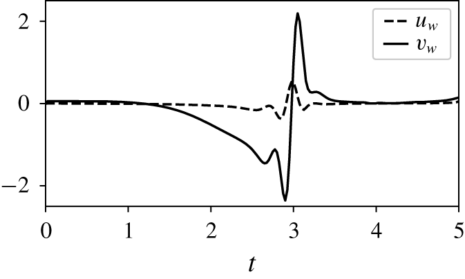
The evolution of the velocity at the wall imposed by control is displayed in figure 12 with some of the same time stamps as in figure 11. It is observed that control initially applies blowing at the centre of the two vortex system  $x\in [0,1]$. After
 $t=2$, suction starts to act, essentially below the vortex, with increasing strength up to
 $t=3$. At this time, the primary vortex has reached its lowest altitude (see figure 11e). Subsequent control essentially reduces to slight blowing at the left of the primary vortex. After
 $t=2$, suction starts to act, essentially below the vortex, with increasing strength up to
 $t=3$. At this time, the primary vortex has reached its lowest altitude (see figure 11e). Subsequent control essentially reduces to slight blowing at the left of the primary vortex. Figure 13 shows the time trace of the control at
 $x=1$, that is, under the descent path of the vortex. The suction then blowing strategy of the control described above is grasped immediately using this plot, along with the dominance of the vertical velocity component upon the lateral component.
Evolution of the optimal control  $\boldsymbol{u}_{w}$ along the control area for different time steps. The thicker borders refer to the same times as those used in figure 4. Solid (respectively dashed) lines represent
 $v_{w}$ (respectively
 $u_{w}$).

Evolution of the optimal control velocity at the wall as a function of time at  $x=1$. Solid (respectively dashed) lines represent
 $v_{w}$ (respectively
 $u_{w}$).

Two main factors have been identified to explain how control physically achieves increased lateral displacement. One is related to (i) delayed separation, which reduces the vortex updraft by secondary vorticity, hence maintaining lower vortex altitude and increased induction effect by image vorticity about the ground, and the other one to (ii) reduced effective friction at the ground to decrease the opposition to the vortex lateral displacement.
The factor (i) relates to the suction that is applied by control in the region  $x\in [1,1.5]$, slightly to the right of the primary vortex. Suction is a generic principle to delay boundary layer separation (Lachmann Reference Lachmann2014). Its interest in the present configuration can be grasped by comparing figure 4, without control, for which the boundary layer separates in the region
 $x\in [1,1.5]$ around time
 $t=2.5$, with figure 11, that yields control and which, as a result of suction, allows a delayed separation, up to time
 $t>4$.
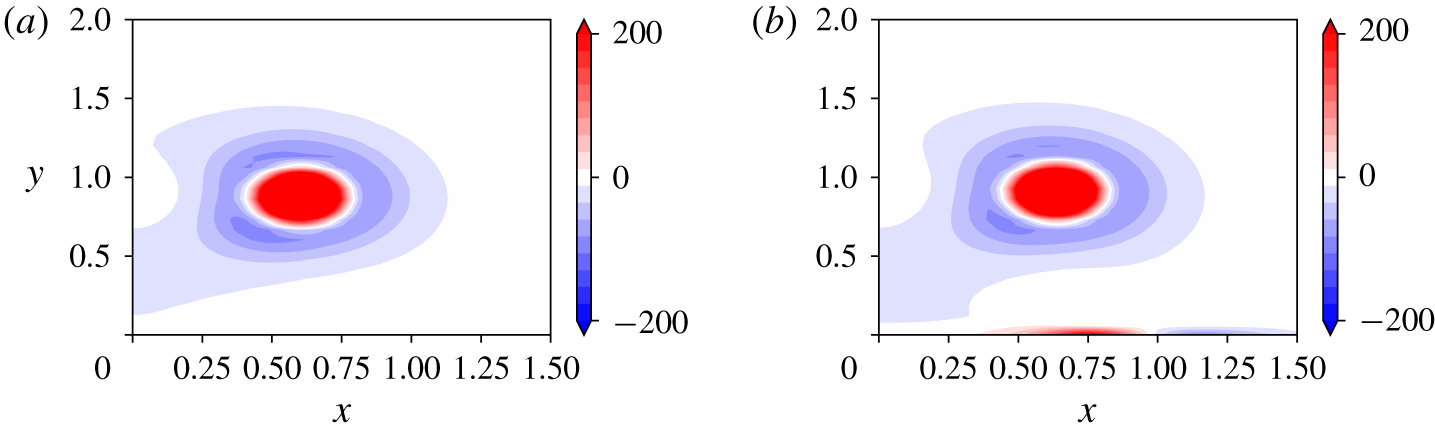
The second factor (ii) is vortex induction. It can be identified using figure 11(d,e), which indicates that a specific vorticity pattern is formed at the wall by control between  $t=2$ and 3, this pattern being absent in the flow at the same time when control is absent (figure 4b). The field of
 $Q$-criterion between the uncontrolled and controlled cases at
 $t=2$ and focused in the region between the primary vortex and the wall is shown in figures 14(a) and 14(b), respectively, to highlight the associated structure. The plot shows that a rotational area is brought about by control which, referring to figure 11(e), amounts to negative vorticity. Albeit the zone does not present a pressure minimum (at least not apparently), for simplicity’s sake we coin it as a vortex. Considering Biot–Savart induction, it can be stated that the effect of this vortex upon the primary vortex favours the motion to the right of the latter, and effectively pushes it along the wall. In the following, this vortex is conveniently referred to as the pusher vortex.
The formation of this pusher vortex can be directly linked to the velocity imposed by the control at the wall. Indeed figure 12 shows that the vertical velocity component generates a strong gradient  $\unicode[STIX]{x2202}v/\unicode[STIX]{x2202}x$ below the primary vortex for time
 $t=2$ to
 $3$ (figure 12d,e) and this is to be analysed as creating the
 $\unicode[STIX]{x1D714}$ associated with the pusher vortex. In effect
 $\unicode[STIX]{x1D714}\simeq \unicode[STIX]{x2202}v/\unicode[STIX]{x2202}x$ since
 $|u_{w}|\ll |v_{w}|$ and characteristic length scales for
 $u_{w}$ and
 $v_{w}$ are similar.
Plot of the  $Q$-criterion at time
 $t=2$ for (a)
 $(1000,5,\infty )$ and (b)
 $(1000,5,1)$. Creation of a rotational area in the boundary layer (positive values of the
 $Q$-criterion) that corresponds to the pusher vortex.

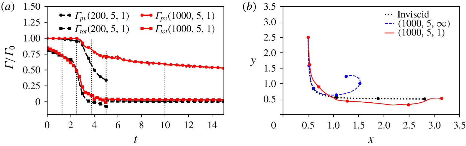
An interesting consequence of control concerns circulation, which is found to be significantly diminished with the application of control. The behaviours of  $\unicode[STIX]{x1D6E4}_{tot}$ and
 $\unicode[STIX]{x1D6E4}_{pv}$ are shown in figure 15(a) for
 $Re=200$ and 1000,
 $T=5$ and
 $l=1$. Comparison can be made with the uncontrolled case in figure 5. For
 $Re=200$, the circulation drops by more than 60 % at
 $t=5$ compared to 50 % after 15 time units in the uncontrolled case. For
 $Re=1000$, the decrease is approximately 15 % compared to less than 10 % in the uncontrolled case, also at
 $t=5$.
Figure 15(b) sums up the previous analysis by showing the trajectory of the controlled vortex against the uncontrolled and inviscid trajectories, with equal time stamps to enable the comparison of the vortex progress in each case. The controlled vortex is initially moved above the uncontrolled trajectory as a consequence of the initial blowing imposed by control. Then, as the uncontrolled vortex rebounds, it moves laterally and close to the ground, reaching an altitude lower than the inviscid hyperbolic path. At the final time, the controlled vortex achieves a more outward position than the inviscid vortex, concluding the efficiency of the blowing/suction strategy.
(a) Evolution of primary vortex and total circulation for  $(200,5,1)$ (black) and
 $(1000,5,1)$ (red). For times beyond
 $t=5$, control has been turned off. (b) Evolution of the centroid trajectories for
 $0\leqslant t\leqslant 5$ for inviscid, controlled
 $(1000,5,1)$ and uncontrolled flow
 $(1000,5,\infty )$. Circled markers correspond to the centroid position at
 $t=0,1,2,3,4,5$.

5.3 Control robustness
In this subsection, we discuss the robustness of the optimal control approach with respect to the initial height, radius and activation time of the control law. It is noteworthy that assessing the robustness of the method with respect to the initial vortex circulation would imply only varying the circulation-based Reynolds number. Previous results comparing  $Re=200$ and 1000 show no major modification of the present strategy with Reynolds number. Three distinct simulations H (for height), R (for radius) and DAT (for delayed activation time) have been carried out where we modify the initial height, dispersion radius and activation time separately. In simulation H, all parameters are kept the same, except for the initial height
 $y_{c_{0}}=5$ (instead of
 $2.5$) and the horizon time (
 $T=10$ instead of 5). Note that doubling the descending distance justifies doubling of the horizon time in order to compare with the case at
 $(1000,5,1)$ and
 $y_{c_{0}}=2.5$. Simulation R keeps all the same parameters as for the case at
 $(1000,5,1)$ except for the initial dispersion radius
 $a=0.1$ (instead of 0.15). In simulation DAT, we use the optimal control law of the optimal case
 $(1000,5,1)$ for the situation when the vortex initially departs from
 $y_{c_{0}}=5$. Control is then only active between
 $t_{a}=2.5$ and
 $t=7.5$. Table 1 summarizes the objective function results and compares them to the reference case
 $(1000,5,1)$,
 $y_{c_{0}}=2.5$ and
 $a=0.15$. The performance of the control, when looking at the value of
 ${\mathcal{J}}_{2}$, is moderately affected for cases H and R, with a relative 18 % decrease, and is unchanged for case DAT. This suggests that the control does not suffer much from changes in the parameters of the present model. The final vorticity fields and time trace of the optimal control at
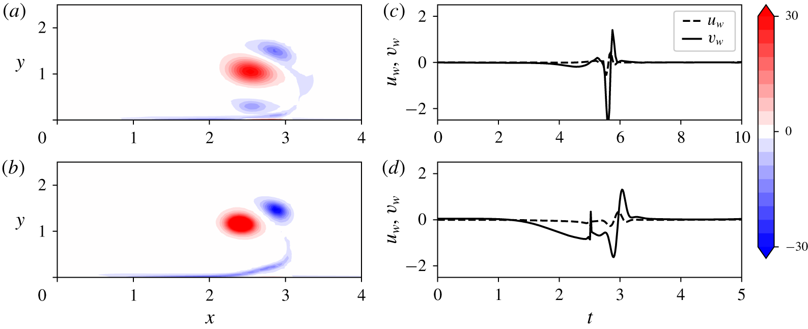
 $x=1$ are shown in figure 16(a,b) for cases H and R. The case DAT leads to negligible changes compared to the reference in figures 11(h) and 13 and is thus not shown in figure 16. Similar behaviours and amplitudes of the cost function are observed between the optimal reference case
 $(1000,5,1)$ and cases H, R and DAT. In particular, the time traces shown in figure 16 resemble those in figure 13(c,d).
Effect of the initial height, radius and activation time on the objective function results. Left column corresponds to the reference optimal case  $(1000,5,1)$ already shown in figure 11. The second, third and fourth columns correspond to simulations H, R and DAT respectively, which yield similar results.


5.4 Vorticity flux at the wall
The physical analysis can be backed by looking theoretically at the evolution of  $I_{1}(t)$, the numerator of
 ${\mathcal{J}}_{1}(t)$, introduced in § 4 (see (4.8)). Following the calculations given in appendix C, the time derivative of
 $I_{1}$ yields
 $$\begin{eqnarray}{\dot{I}}_{1}=-{\displaystyle \frac{2}{Re}}\int _{\unicode[STIX]{x1D6FA}}x|\unicode[STIX]{x1D735}\unicode[STIX]{x1D714}|^{2}\,\text{d}\unicode[STIX]{x1D6FA}+{\displaystyle \frac{1}{Re}}\int _{\unicode[STIX]{x2202}\unicode[STIX]{x1D6FA}_{1}}x(\unicode[STIX]{x1D735}\unicode[STIX]{x1D714}^{2})\boldsymbol{\cdot }\boldsymbol{n}\,\text{d}x+\int _{\unicode[STIX]{x1D6FA}}u\unicode[STIX]{x1D714}^{2}\,\text{d}\unicode[STIX]{x1D6FA}={\dot{I}}_{11}+{\dot{I}}_{12}+{\dot{I}}_{13}.\end{eqnarray}$$
This equation shows that  $I_{1}$ is reduced by the dissipative term (
 ${\dot{I}}_{11}$), and increased by the vorticity flux at the bottom boundary (
 ${\dot{I}}_{12}$) which also can be written as
 $$\begin{eqnarray}{\dot{I}}_{12}=-\frac{2}{Re}\int _{\unicode[STIX]{x2202}\unicode[STIX]{x1D6FA}_{1}}x\unicode[STIX]{x1D714}\frac{\unicode[STIX]{x2202}\unicode[STIX]{x1D714}}{\unicode[STIX]{x2202}y}\,\text{d}x,\end{eqnarray}$$
and by the advection of the vorticity field ( ${\dot{I}}_{13}$).
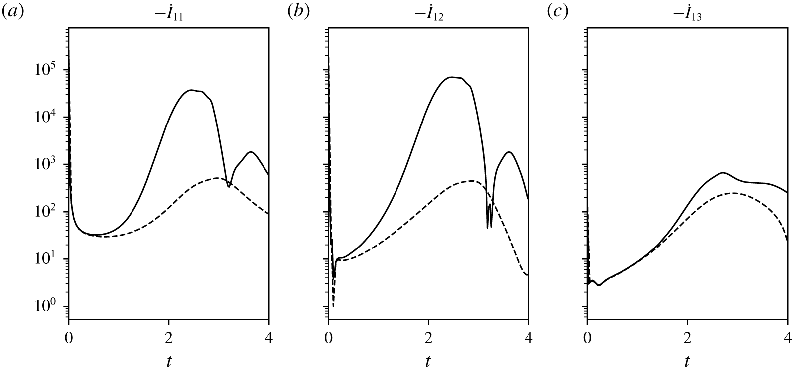
Figure 17 plots the evolution of  ${\dot{I}}_{11,12,13}$ for the controlled and uncontrolled cases at
 $Re=1000$. The term
 ${\dot{I}}_{13}$ is almost unaffected by control, unlike the terms
 ${\dot{I}}_{11}$ and
 ${\dot{I}}_{12}$, which are increased by nearly 3 orders of magnitude when reaching their maximum values (shortly after
 $t=2$). The term
 ${\dot{I}}_{12}$ becomes larger than
 ${\dot{I}}_{11}$, which implies the net increase of
 $I_{1}$ and also means that the vorticity flux provoked by control at the wall, which results in the negative pusher vortex being present there, is the dominant mechanism at
 $Re=1000$. As explained previously, this pusher vortex creates a horizontal induction to the primary vortex which minimizes the impact of zero velocity at the wall. This way, it allows the primary vortex to slide along the wall and move to larger lateral distances.
Time evolution  $-{\dot{I}}_{11},{\dot{I}}_{12},{\dot{I}}_{13}$ from left to right for the uncontrolled case (dashed lines) and the controlled case (solid lines) for
 $(Re,T,l)=(1000,4,10)$.

6 Conclusion
This work shows the effective control of vortex rebound at the ground in the situation of a laminar set of two opposite symmetric vortices, in a quiescent environment. The physics of vortex rebound results from the interplay between the vortex and the boundary layer it induces. An optimal control approach is employed with mass flow exchange at the wall to counteract this rebound and allow for a larger lateral displacement of the vortex, a concept initially devised for the interest of wake vortices in airport airfields. At the same time, the optimization offers novel insights into the dynamics of vortices impacting the ground and the effective physical leverages for its modification. The optimal blowing/suction strategy is shown to target a delayed separation of the boundary layer formed at the wall by a predominant suction of the flow ahead of the vortex, and the formation of a pusher vortex, of opposite sign vorticity compared to the primary vortex, to reduce the no-slip constraint at the wall. This helps the lateral movement of the vortex by mutual induction by the inserted vortex. Importantly, it is found that blowing laterally to the wall is essentially not required. In the most efficient control case, the lateral movement of the vortex is almost doubled, reaching a larger lateral distance than without viscosity. At the lower Reynolds number  $Re=200$ envisaged in this study, the control is also found to suppress the vortex. From a broader point of view, the findings of the present analysis show perspectives for vortex control of the coherent structures embedded in wall turbulence, in line with the conclusions of Akhavan et al. (Reference Akhavan, Jung and Mangiavacchi1993), Choi et al. (Reference Choi, Moin and Kim1994) and Lee et al. (Reference Lee, Kim, Babcock and Goodman1997), all the more so as the Reynolds number range targeted here is coherent with this type of flow.
For the problem of airport and airport terminal management (ATM), the effectiveness of the control potentially makes it an appealing strategy to apply ahead of runways to reduce vortex encounter. From a technical point of view, blowing and sucking at the ground could be achieved by compressed air supply and sucking devices (e.g. vacuum chambers or ejector suction devices) wrapped into a web of holes on the ground, vertically oriented, and a controller system for the multiple valves involved. This would still represent a great technical challenge. Moreover, in spite of the apparent generality of the mechanisms exposed in the present study, there are also physical questions on the variety of situations that could be tackled by such a system. Further analysis of the effect of turbulence, presence of wind, thermal updrafts and terrain effects to name a few would be necessary to fully qualify the robustness of the control strategy. Some of these questions could be answered by carrying out higher Reynolds number simulations of the control laws developed here, including possibly variations in the boundary conditions to incorporate, e.g. side wind. Note, however, that the effect of Reynolds number on the early stages of vortex dynamics is small, which justifies the choice of low Reynolds analysis performed here, but becomes important for the development of turbulence in the boundary layer flow at the ground and turbulent interactions with the vortex. As it is, the current algorithm stands as a proof of concept that shows both the physical interest in optimizing what happens at the ground and the working of the control in a simple configuration.
Another side question on the application of the concept is that of parallel runways. Indeed, as the vortices are pushed to the sides, they may interfere with the nearby runway. The lateral distances realized in the present work are of the order of 3 to 4 wingspans at most (we neglect here the ratio between vortex separation and wingspan, as it is close to unity). A non-exhaustive list of some 86 airports that operate parallel runways is available in libraries dedicated to flight safety (see for instance Skybrary (2019)). For airports with parallel runways far apart, such as London Heathrow airport, the matter is not a question. For airports with nearby runways, such as Philadelphia International airport, the question becomes important as the separation distance, in this case approximately 400 m, ranges between 10 wingspans for small airliners to 5 for heavy ones. In the present analysis however, it is found that as the vortex control stops, the vortex rebounds and almost stops its sideward motion. This means that the control concept could certainly cope with an additional constraint of maximum lateral distance for the vortex system.
At this stage certainly one of the most interesting discussions is on the cost of the control. Using the normalization on  $\unicode[STIX]{x1D6E4}_{0}$ and
 $b$ used in the present study, the power
 $P$ required to apply control can be evaluated by integrating the flux of kinetic energy at the wall, that is
 $$\begin{eqnarray}P=\int _{0}^{T}\int _{\unicode[STIX]{x2202}\unicode[STIX]{x1D6FA}_{1}}|\boldsymbol{u}_{w}|^{2}v_{w}\,\text{d}x\,\text{d}t.\end{eqnarray}$$
This quantity scales with  $\unicode[STIX]{x1D70C}\unicode[STIX]{x1D6E4}_{0}^{3}/(16\unicode[STIX]{x03C0}^{3}b^{2})$ hence, for a typical large aircraft (
 $b=50~\text{m}$,
 $\unicode[STIX]{x1D6E4}_{0}=500~\text{m}^{2}~\text{s}^{-1}$), this would yield
 $P\simeq 100~\text{W}~\text{m}^{-1}$ (the integrated quantity is order one). The set-up being two-dimensional, control must be applied over an a priori infinite distance. In practice, the control area would be finite yet the questions of what length of application would be necessary is open. There would also be different constraints when considering departing or arriving aircraft. This would deserve a detailed analysis and especially require three-dimensional effects to be looked into.
One certainly interesting use of the proposed control would be to exploit the capacity to move the vortex normal to its axis to induce three-dimensional waves along the vortex. This could be obtained by modulating the control in the axial direction or even implementing only crenelated patches of control. Besides drastically decreasing the required power, this would help three-dimensional instabilities that naturally grow in the wake (Williamson et al. Reference Williamson, Leweke, Asselin and Harris2014). Indeed, the range of horizon times  $T=0..10$ contains the characteristic times of Crow and elliptic instabilities, respectively
 $T_{cr}\simeq 6$ (Williamson et al. Reference Williamson, Leweke, Asselin and Harris2014) and
 $T_{el}\simeq 4.9$ (Widnall, Bliss & Tsai Reference Widnall, Bliss and Tsai1974; Leweke & Williamson Reference Leweke and Williamson1998; Sipp & Jacquin Reference Sipp and Jacquin2003). Such an opportunity could be usefully investigated in future works with the question of the optimal wavelength to be applied in mind.
Other perspectives are opened up by this work. One interesting outlook concerns the control of the shape of the wall instead of that of the boundary condition for the velocity field. Using the same technique that has been applied in the present study, the optimization of the shape of the wall to achieve the increased lateral displacement of the vortex or more simply to target its reduction could be envisaged. As a first step toward such an approach the present results can be used to derive such wall deformations since  $(u_{w},v_{w})=(\unicode[STIX]{x2202}x_{w}/\unicode[STIX]{x2202}t,\unicode[STIX]{x2202}y_{w}/\unicode[STIX]{x2202}t)$ can relate the movement of the wall to the velocity imposed at its surface. However, this approach would not take into account the effect of surface deformation on the flow and would hence be suited to very small surface deformations. For large displacements, new developments would be required to incorporate the deformation of the numerical domain (mesh) in the procedure. Like the blowing/suction strategy, adaptive walls could be an issue in practice due to implementation complexity. A way to deal with this would be to consider a static shape to control the vortices, in a way similar to what has been achieved at Amsterdam airport to counter the noise of aircraft (Sorvig & Thompson Reference Sorvig and Thompson2018). The optimization procedure in this case would not require the use of the adjoint technique since the shape of the wall could be described by a small set of parameters. Another way could be the use of compliant walls. The subject has gained strong interest in recent years to deal with hydro and aerodynamic problems such as drag reduction (Endo & Himeno Reference Endo and Himeno2002), flow instabilities (Yeo Reference Yeo1992; Davies & Carpenter Reference Davies and Carpenter1997; Hoepffner, Bottaro & Favier Reference Hoepffner, Bottaro and Favier2010) and turbulence (Luhar, Sharma & McKeon Reference Luhar, Sharma and McKeon2015). In particular, Endo & Himeno (Reference Endo and Himeno2002) shows that passive compliant walls tend to reduce the intensity of vortex structures at the wall.
Acknowledgements
This work was granted access to the HPC resources IDRIS under the allocation 2016-100746 made by GENCI. The work is primarily supported by the PHYWAKE project dedicated to vortex dynamics and funded by the French Directorate for Civil Aviation (DGAC). The careful reading and support of Navrose have been deeply appreciated and were decisive to finalize this work.
Declaration of interests
The authors report no conflict of interest.
Appendix A. Compatibility equation
The derivation leading to the compatibility (4.7) is here derived. Without loss of generality let us consider three-dimensional fields. We introduce the following inner spatial product:
 $$\begin{eqnarray}\langle \boldsymbol{f}(\boldsymbol{x}),\boldsymbol{g}(\boldsymbol{x})\rangle =\int _{\unicode[STIX]{x1D6FA}}\boldsymbol{f}(\boldsymbol{x})\boldsymbol{\cdot }\boldsymbol{g}(\boldsymbol{x})\,\text{d}\unicode[STIX]{x1D6FA},\end{eqnarray}$$
where  $\boldsymbol{f}$ and
 $\boldsymbol{g}$ are functions of space. By cancelling the first variation of the Lagrangian function (4.4) with respect to
 $\boldsymbol{u}(T)$, one obtains
 $$\begin{eqnarray}\left\langle {\displaystyle \frac{\unicode[STIX]{x2202}{\mathcal{L}}}{\unicode[STIX]{x2202}\boldsymbol{u}(T)}},\unicode[STIX]{x1D739}\boldsymbol{u}(T)\right\rangle =\left\langle {\displaystyle \frac{\unicode[STIX]{x2202}{\mathcal{J}}}{\unicode[STIX]{x2202}\boldsymbol{u}(T)}},\unicode[STIX]{x1D739}\boldsymbol{u}(T)\right\rangle -\left\langle \boldsymbol{u}^{+}(T),\unicode[STIX]{x1D739}\boldsymbol{u}(T)\right\rangle =0,\end{eqnarray}$$
where  $\unicode[STIX]{x1D739}\boldsymbol{u}(T)$ is an arbitrary vector. To compute the term
 $\left\langle (\unicode[STIX]{x2202}{\mathcal{J}}/\unicode[STIX]{x2202}\boldsymbol{u}(T)),\unicode[STIX]{x1D739}\boldsymbol{u}(T)~\right\rangle$, one needs to compute
 $\left\langle (\unicode[STIX]{x2202}I_{m}/\unicode[STIX]{x2202}\boldsymbol{u}(T)),\unicode[STIX]{x1D739}\boldsymbol{u}(T)\right\rangle$ where
 $I_{m=0,1}$ is defined in (4.8) and (4.9). For the sake of clarity, let us rewrite
 $I_{m}$ with the following expression:
 $$\begin{eqnarray}I_{m}(\boldsymbol{u}(T))=\int _{V}x^{m}(\unicode[STIX]{x1D735}\times ~\boldsymbol{u}(T))^{2}\,\text{d}\unicode[STIX]{x1D6FA}.\end{eqnarray}$$
This allows us to compute the directional derivative of  $I_{m}$ with respect to
 $\boldsymbol{u}(T)$ as follows:
 $$\begin{eqnarray}\left\langle {\displaystyle \frac{\unicode[STIX]{x2202}I_{m}}{\unicode[STIX]{x2202}\boldsymbol{u}(T)}},\unicode[STIX]{x1D739}\boldsymbol{u}(T)\right\rangle =\lim _{\unicode[STIX]{x1D716}\rightarrow 0}{\displaystyle \frac{1}{\unicode[STIX]{x1D716}}}(I_{m}(\boldsymbol{u}+\unicode[STIX]{x1D716}\unicode[STIX]{x1D739}\boldsymbol{u}(T))-I_{m}(\boldsymbol{u})),\end{eqnarray}$$
yielding
 $$\begin{eqnarray}\left\langle {\displaystyle \frac{\unicode[STIX]{x2202}I_{m}}{\unicode[STIX]{x2202}\boldsymbol{u}(T)}},\unicode[STIX]{x1D739}\boldsymbol{u}(T)\right\rangle =\int _{\unicode[STIX]{x1D6FA}}2x^{m}\unicode[STIX]{x1D74E}(T)\boldsymbol{\cdot }(\unicode[STIX]{x1D735}\times \unicode[STIX]{x1D739}\boldsymbol{u}(T))\,\text{d}\unicode[STIX]{x1D6FA}.\end{eqnarray}$$
We can use the following formula  $\unicode[STIX]{x1D735}\boldsymbol{\cdot }(\boldsymbol{a}\times \boldsymbol{b})=\boldsymbol{b}\boldsymbol{\cdot }(\unicode[STIX]{x1D735}\times \boldsymbol{a})-\boldsymbol{a}\boldsymbol{\cdot }(\unicode[STIX]{x1D735}\times \boldsymbol{b})$ and integration over
 $\unicode[STIX]{x1D6FA}$ using the Green–Ostrogradski theorem, which yields
 $$\begin{eqnarray}\left\langle {\displaystyle \frac{\unicode[STIX]{x2202}I_{m}}{\unicode[STIX]{x2202}\boldsymbol{u}(T)}},\unicode[STIX]{x1D739}\boldsymbol{u}(T)~\right\rangle =\int _{\unicode[STIX]{x1D6FA}}\unicode[STIX]{x1D735}\times (2x^{m}\unicode[STIX]{x1D74E})\boldsymbol{\cdot }\unicode[STIX]{x1D739}\boldsymbol{u}(T)\,\text{d}\unicode[STIX]{x1D6FA}.\end{eqnarray}$$
Remark that the previous equality holds true for any arbitrary vector  $\unicode[STIX]{x1D739}\boldsymbol{u}(T)$, thus
 $$\begin{eqnarray}{\displaystyle \frac{\unicode[STIX]{x2202}I_{m}}{\unicode[STIX]{x2202}\boldsymbol{u}(T)}}=\unicode[STIX]{x1D735}\times (2x^{m}\unicode[STIX]{x1D74E})=2\unicode[STIX]{x1D735}(x^{m})\times \unicode[STIX]{x1D74E}+2x^{m}\unicode[STIX]{x1D735}\times \unicode[STIX]{x1D74E}.\end{eqnarray}$$
Hence, one can evaluate the initialization of the adjoint variable in two dimensions
 $$\begin{eqnarray}\boldsymbol{u}^{+}(T)={\displaystyle \frac{\unicode[STIX]{x2202}{\mathcal{J}}}{\unicode[STIX]{x2202}\boldsymbol{u}(T)}}={\displaystyle \frac{2}{I_{0}(T)}}(x\unicode[STIX]{x1D735}\times \unicode[STIX]{x1D714}(T)\boldsymbol{e}_{z}+\unicode[STIX]{x1D735}x\times \unicode[STIX]{x1D714}(T)\boldsymbol{e}_{z})-{\displaystyle \frac{2I_{1}(T)}{I_{0}(T)^{2}}}(\unicode[STIX]{x1D735}\times \unicode[STIX]{x1D714}(T)\boldsymbol{e}_{z}),\end{eqnarray}$$
and find (4.7).
Appendix B. Convergence analysis
B.1 Optimization
This appendix provides examples of the convergence of the algorithm described in § 4. The assessment of numerical convergence is evaluated using the following residual
 $$\begin{eqnarray}r_{n}=\displaystyle \left|{\displaystyle \frac{{\mathcal{J}}_{n}-{\mathcal{J}}_{n-1}}{{\mathcal{J}}_{n}}}\right|.\end{eqnarray}$$
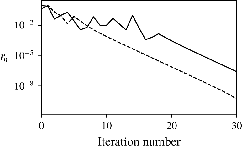
Figure 18 plots  $r_{n}$ as a function of iteration number and displays two typical convergence results: approximately 20 iterations are required to obtain a well-converged optimal (
 $r_{n}\simeq 10^{-3}$).
Convergence for two typical cases  $(200,4,1)$ (dashed line) and
 $(1000,4,1)$ (solid line) showing algorithmic convergence.

B.2 Influence of the interpolation time interval  $\unicode[STIX]{x1D6FF}t_{i}$

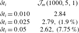
This appendix discusses the convergence as a function of  $\unicode[STIX]{x1D6FF}t_{i}$. One example is considered:
 $(Re,T,l)=(1000,5,1)$. Convergence results are provided in table 2. The value
 $\unicode[STIX]{x1D6FF}t_{i}=0.025$ is chosen as a consequence of the satisfactory convergence it enables.
Convergence analysis of the  $\unicode[STIX]{x1D6FF}t_{i}$ used for the interpolation procedure detailed in (4.11).

Appendix C. Temporal evolution of the cost function
This appendix details the derivation of relation (4.4). We consider the general case of  $I_{m}=\int _{\unicode[STIX]{x1D6FA}}{\mathcal{A}}_{m}\,\text{d}V$ with
 ${\mathcal{A}}_{m}=x^{m}\unicode[STIX]{x1D714}^{2}$ and
 $m=0,1$. The time derivative of
 $I_{m}$ is obtained as follows:
 $$\begin{eqnarray}{\dot{I}}_{m}={\displaystyle \frac{\text{d}}{\text{d}t}}\int _{\unicode[STIX]{x1D6FA}}{\mathcal{A}}_{m}\,\text{d}V=\int _{\unicode[STIX]{x1D6FA}}{\displaystyle \frac{\unicode[STIX]{x2202}{\mathcal{A}}_{m}}{\unicode[STIX]{x2202}t}}\,\text{d}V+\int _{\unicode[STIX]{x2202}\unicode[STIX]{x1D6FA}}{\mathcal{A}}_{m}(\boldsymbol{u}\boldsymbol{\cdot }\boldsymbol{n})\,\text{d}S=\int _{\unicode[STIX]{x1D6FA}}{\displaystyle \frac{\unicode[STIX]{x2202}{\mathcal{A}}_{m}}{\unicode[STIX]{x2202}t}}\,\text{d}V+\int _{\unicode[STIX]{x1D6FA}}\unicode[STIX]{x1D735}\boldsymbol{\cdot }({\mathcal{A}}_{m}\boldsymbol{u})\,\text{d}V.\end{eqnarray}$$
The last term of the previous equation develops into  ${\mathcal{A}}_{m}\unicode[STIX]{x1D735}\boldsymbol{\cdot }(\boldsymbol{u})+\boldsymbol{u}\boldsymbol{\cdot }\unicode[STIX]{x1D735}({\mathcal{A}}_{m})=\boldsymbol{u}\boldsymbol{\cdot }\unicode[STIX]{x1D735}({\mathcal{A}}_{m})=mx^{m-1}u\unicode[STIX]{x1D714}^{2}+x^{m}(\boldsymbol{u}\boldsymbol{\cdot }\unicode[STIX]{x1D735})\unicode[STIX]{x1D714}^{2}$. The vorticity equations in two dimensions are written as
 $$\begin{eqnarray}\frac{\unicode[STIX]{x2202}\unicode[STIX]{x1D714}}{\unicode[STIX]{x2202}t}+(\boldsymbol{u}\boldsymbol{\cdot }\unicode[STIX]{x1D735})\unicode[STIX]{x1D714}={\displaystyle \frac{1}{Re}}\unicode[STIX]{x0394}\unicode[STIX]{x1D714}.\end{eqnarray}$$
This is used to simplify (C 1)
 $$\begin{eqnarray}{\dot{I}}_{m}=\int _{\unicode[STIX]{x1D6FA}}2\unicode[STIX]{x1D714}x^{m}\left\{\frac{\unicode[STIX]{x2202}\unicode[STIX]{x1D714}}{\unicode[STIX]{x2202}t}+(\boldsymbol{u}\boldsymbol{\cdot }\unicode[STIX]{x1D735})\unicode[STIX]{x1D714}\right\}+mx^{m-1}u\unicode[STIX]{x1D714}^{2}\,\text{d}V=\int _{\unicode[STIX]{x1D6FA}}{\displaystyle \frac{2}{Re}}x^{m}\unicode[STIX]{x1D714}\unicode[STIX]{x0394}\unicode[STIX]{x1D714}+mx^{m-1}u\unicode[STIX]{x1D714}^{2}\,\text{d}V.\end{eqnarray}$$
The term  $x^{m}\unicode[STIX]{x1D714}\unicode[STIX]{x0394}\unicode[STIX]{x1D714}$ can be worked out using the identity
 $\unicode[STIX]{x1D735}\boldsymbol{\cdot }(f\unicode[STIX]{x1D735}(g))=\unicode[STIX]{x1D735}(f)\boldsymbol{\cdot }\unicode[STIX]{x1D735}(g)+f\unicode[STIX]{x0394}g$ which yields
 $$\begin{eqnarray}{\dot{I}}_{m}={\displaystyle \frac{2}{Re}}\int _{\unicode[STIX]{x1D6FA}}\unicode[STIX]{x1D735}\boldsymbol{\cdot }(x^{2}\unicode[STIX]{x1D714}\unicode[STIX]{x1D735}\unicode[STIX]{x1D714})-\unicode[STIX]{x1D735}(x^{m}\unicode[STIX]{x1D714})\boldsymbol{\cdot }\unicode[STIX]{x1D735}\unicode[STIX]{x1D714}+mx^{m-1}u\unicode[STIX]{x1D714}^{2}\,\text{d}V.\end{eqnarray}$$
Then, the middle term of (C 3) can be developed and integrated. This gives
 $$\begin{eqnarray}{\dot{I}}_{m}={\displaystyle \frac{2}{Re}}\int _{\unicode[STIX]{x1D6FA}}\unicode[STIX]{x1D735}\boldsymbol{\cdot }(x^{2}\unicode[STIX]{x1D714}\unicode[STIX]{x1D735}\unicode[STIX]{x1D714})-x^{m}\unicode[STIX]{x1D735}(\unicode[STIX]{x1D714})^{2}+mx^{m-1}u\unicode[STIX]{x1D714}^{2}\,\text{d}V.\end{eqnarray}$$
Eventually, using the Green–Ostrogradski theorem, we get
 $$\begin{eqnarray}{\dot{I}}_{m}={\displaystyle \frac{2}{Re}}\int _{\unicode[STIX]{x1D6FA}}-x^{m}|\unicode[STIX]{x1D735}\unicode[STIX]{x1D714}|^{2}\,\text{d}V+{\displaystyle \frac{1}{Re}}\int _{\unicode[STIX]{x2202}\unicode[STIX]{x1D6FA}}x^{m}(\unicode[STIX]{x1D735}\unicode[STIX]{x1D714}^{2})\boldsymbol{\cdot }\boldsymbol{n}\,\text{d}S+\int _{\unicode[STIX]{x1D6FA}}mx^{m-1}u\unicode[STIX]{x1D714}^{2}\,\text{d}V.\end{eqnarray}$$
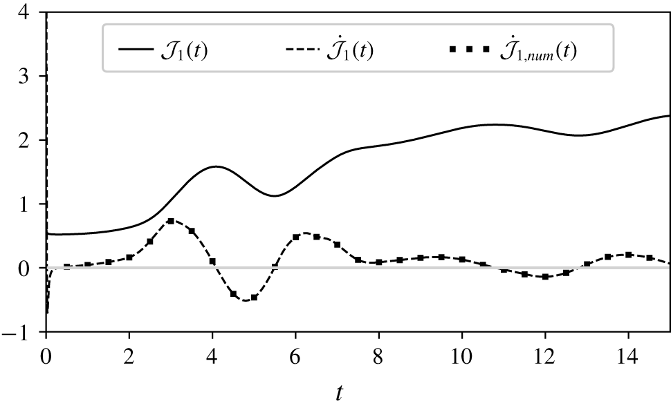
In figure 19 the time evolution of the cost functional along with its derivative for the uncontrolled case  $(Re,T,l)=(1000,15,\infty )$ are shown. The derivative is obtained either by using (C 6) leading to
 $\dot{{\mathcal{J}}}=({\dot{I}}_{1}I_{0}-I_{1}{\dot{I}}_{1})/I_{0}^{2}$ or by numerically differentiating
 ${\mathcal{J}}(t)$. The two approaches to the differentiation match well.
Time evolution of  ${\mathcal{J}}_{1}$ (solid line) and
 $\dot{{\mathcal{J}}_{1}}$ (dashed line) computed with (C 6) for the
 $(Re,T,l)=(1000,15,\infty )$ case. Circled markers, placed every 2000 points, correspond to the numerical time differentiation of
 ${\mathcal{J}}_{1}$ (denoted
 $\dot{{\mathcal{J}}}_{1,num}$) matching the analytical expression of
 $\dot{{\mathcal{J}}_{1}}$.