1 Introduction
A vast amount of research has been dedicated to the understanding of fluid–structure interaction (FSI) because of its practical significance in many fields. For example, fluid flow can induce structural vibration as a result of the formation of alternately shedding vortices into the wake, which is known as flow-induced vibration. If the vibration triggers resonance, then the structure may suffer fatigue or even catastrophic failure. Vortex-induced vibration or VIV is a periodic flow-induced vibration state. VIV can be identified with vibrations that occur through the synchronisation of the structural response with the wake unsteadiness (i.e. vortex shedding) when the frequency is close to the system’s natural frequency. The occurrence of VIV can be found for structures such as bridges, chimney stacks, cables, air planes, ground vehicles, submarines and marine vessels, when there is a relative motion between the fluid and the solid structure. Therefore, it is important to study the nature of vortex-induced vibration and its mechanisms as a means for its control.
The fundamentals of VIV have been studied substantially through experimental and numerical research studies focusing on basic geometries, many of which are discussed in the comprehensive reviews of Bearman (Reference Bearman1984), Parkinson (Reference Parkinson1989), Sarpkaya (Reference Sarpkaya2004), Williamson & Govardhan (Reference Williamson and Govardhan2004, Reference Williamson and Govardhan2008) and Wu, Ge & Hong (Reference Wu, Ge and Hong2012). Most of these studies were based on cylindrical structures due to their intrinsic engineering importance and due to the simplicity of setting up such models, both experimentally and computationally. For VIV of a cylinder, three distinct branches (initial, upper and lower) have been observed in the vibration amplitude response curve
 $A^{\ast }(U^{\ast })$
, where
 $A^{\ast }$
is the non-dimensional vibration amplitude and
 $U^{\ast }$
is the reduced velocity. Govardhan & Williamson (Reference Govardhan and Williamson2000) revealed that the first transition involved a jump in the ‘vortex phase’, related to the changing dynamics of vortex forcing in the transition between
 $2S$
and
 $2P$
shedding wake modes; the second transition involved a jump in the ‘total phase’.
Compared to VIV of a cylinder, fewer studies have been devoted to developing an understanding of VIV of a sphere, despite the fact that there is an abundance of applications involving spherical bodies. For example, tethered bodies such as buoys, underwater mines, tethered balloons and towed objects behind vessels. A series of experimental studies conducted by Govardhan & Williamson (Reference Govardhan and Williamson1997), Williamson & Govardhan (Reference Williamson and Govardhan1997), Jauvtis, Govardhan & Williamson (Reference Jauvtis, Govardhan and Williamson2001) and Govardhan & Williamson (Reference Govardhan and Williamson2005) using tethered spheres subject to one or two degrees of freedom (DOF) motion revealed that a sphere also showed a VIV behaviour with a large oscillation amplitude, similar to that of a cylinder. Furthermore, they observed four different modes of vibrations (named modes I–IV) with varying characteristics in terms of sphere oscillation amplitude and phase, and wake structures. The first two modes of oscillation appeared within the reduced-velocity range
 $5\lesssim U^{\ast }\lesssim 10$
. For these two modes, the body oscillation frequency,
 $f$
, was close to the natural vortex-shedding frequency,
 $f_{vor}$
, and the system’s natural frequency,
 $f_{n}$
; this indeed suggested that these two modes of vibration were vortex-induced vibration. A similar observation was reported over the reduced velocity range,
 $3\lesssim U^{\ast }\lesssim 14$
by Hout, Katz & Greenblatt (Reference Hout, Katz and Greenblatt2013) and Krakovich, Eshbal & Hout (Reference Krakovich, Eshbal and Hout2013) in their investigations of VIV of a tethered sphere. The sphere response amplitude smoothly transitioned from mode I to mode II, in contrast to the VIV response of a cylinder, which displays discontinuous branches in the amplitude response curve. Govardhan & Williamson (Reference Govardhan and Williamson2005) identified that there was a smooth
 ${\sim}90^{\circ }$
phase difference in vortex phase (the phase between the vortex force and the sphere displacement) between mode I and mode II. In these two modes, they found that two-sided hairpin-type vortex loops were shedding into the wake as the sphere vibrated. Moreover, there was a change in timing of vortex shedding relative to the sphere motion once it passed from mode I to mode II, which was consistent with their observation of the change in vortex phase.
Following the mode II vibration as the reduced velocity was increased, Jauvtis et al. (Reference Jauvtis, Govardhan and Williamson2001) observed mode III vibration began at a reduced velocity
 $U^{\ast }\sim 20$
–
 $40$
with heavy spheres of
 $m^{\ast }=80$
and
 $940$
. In contrast to modes I and II, the principal vortex-shedding frequency for mode III vibration was three to eight times higher than the sphere vibration frequency (Jauvtis et al.
Reference Jauvtis, Govardhan and Williamson2001). Therefore, mode III vibration was difficult to explain by classical lock-in theories. However, Govardhan & Williamson (Reference Govardhan and Williamson2005) argued that if the body were to be perturbed, it could generate a self-sustaining vortex force that could be sustained over multiple shedding cycles, leading to body vibrations of large amplitudes. They categorised mode III as movement-induced excitation (Naudascher & Rockwell Reference Naudascher and Rockwell2012). In this mode of vibration, Govardhan & Williamson (Reference Govardhan and Williamson2005) observed that there is an underlying streamwise vortex structure, which is synchronised with the sphere vibration frequency, enabling highly periodic vibration. Consistently, they observed long vortex-loop structures. Subsequently, Jauvtis et al. (Reference Jauvtis, Govardhan and Williamson2001) observed mode IV vibration, at very high reduced velocities (
 $U^{\ast }>100$
). In this mode, the sphere oscillation frequency was not periodic as it was in the first three modes, but interestingly, the vibration frequency was very close to the natural frequency of the system.
Apart from those experimental studies, a few numerical studies have also been reported on VIV of a sphere. Pregnalato (Reference Pregnalato2003) investigated the VIV of a tethered sphere at the Reynolds number
 $500$
with two different mass ratios (
 $m^{\ast }=0.8$
, and
 $0.082$
). In that numerical study, he observed modes II–IV vibrations that had been observed in the experimental studies of Jauvtis et al. (Reference Jauvtis, Govardhan and Williamson2001). In the higher mass-ratio case, mode II appeared in the reduced-velocity range,
 $U^{\ast }\approx 5$
–
 $10$
, while modes III and IV appeared for
 $U^{\ast }>10$
. However, for the lower mass-ratio case, mode IV vibration did not appear in the reduced-velocity range studied (
 $U^{\ast }=0$
–
 $20$
). Therefore, he suspected that there exists a critical mass for mode IV VIV of a sphere to occur. More recently, Lee, Thompson & Hourigan (Reference Lee, Thompson, Hourigan, Denier, Finn and Mattner2008) and Lee, Hourigan & Thompson (Reference Lee, Hourigan and Thompson2013) investigated the VIV of a neutrally buoyant (
 $m^{\ast }=1$
) tethered sphere, which was constrained to move on a spherical surface. This was a combined numerical and experimental study that covered the Reynolds number range
 $Re=50$
–
 $12\,000$
. They found there to be seven different broad and relatively distinct sphere oscillation and wake states.
Behara, Borazjani & Sotiropoulos (Reference Behara, Borazjani and Sotiropoulos2011) investigated VIV of a sphere allowing 3 DOF movement at a Reynolds number of
 $300$
and reduced mass of
 $2$
, for the reduced-velocity range
 $4\leqslant U^{\ast }\leqslant 9$
. In their study, the sphere showed two different amplitude responses, corresponding to two different wake states at the same reduced velocity. In one case, the sphere moved in a circular orbit with a spiral-type wake shedding behind the sphere. In the other case, the sphere vibrated in a plane with hairpin-type vortex loops shedding behind the sphere. They observed two different amplitude response curves corresponding to each case. The sphere oscillation amplitude was smaller when it moved in a circular orbit compared to the planar state. In addition, they observed hysteresis in the response when the sphere was moving in a circular orbit at the beginning of the synchronisation regime. This study was extended by Behara & Sotiropoulos (Reference Behara and Sotiropoulos2016) by expanding the reduced-velocity range to
 $0\leqslant U^{\ast }\leqslant 13$
, and by varying the Reynolds number of the flow from
 $Re=300$
to
 $1000$
for one fixed reduced-velocity case (
 $U^{\ast }=9$
). It was found that the sphere trajectories were strongly dependent on the Reynolds number.
The effect of the rotational motion on bluff bodies has been investigated for centuries. Early research studies carried out by Robins in the eighteenth century (Robins Reference Robins1972) and Magnus in the nineteenth century (Magnus Reference Magnus1853) revealed that a bluff body experiences a lift force (‘Magnus force’) when it propagates with a transverse rotation. Later in the twentieth century, researchers investigated the effect of the rotation rate,
 $\unicode[STIX]{x1D6FC}=\unicode[STIX]{x1D714}D/2U$
, of a sphere on the drag and lift forces (
 $F_{d}$
and
 $F_{l}$
), where
 $\unicode[STIX]{x1D714}$
is the angular speed of the sphere,
 $D$
is the diameter of the sphere and
 $U$
is the free-stream velocity of the flow. Rubinow & Keller (Reference Rubinow and Keller1961) derived an expression for the lift force acting on a transversely rotating sphere for the Stokes regime (
 $Re\leqslant 1$
and
 $\unicode[STIX]{x1D6FC}\leqslant 0.01$
). They found that the drag force was independent of the rotation rate and that the lift coefficient,
 $C_{l}=F_{l}/(0.5\unicode[STIX]{x1D70C}_{f}U\unicode[STIX]{x03C0}(D/2)^{2})$
, could be expressed as
 $2\unicode[STIX]{x1D6FC}$
. Kurose & Komori (Reference Kurose and Komori1999) considered the flow regimes
 $1\leqslant Re\leqslant 500$
and
 $0\leqslant \unicode[STIX]{x1D6FC}\leqslant 0.25$
, and found that both drag and lift forces increased with the rotation rate.
In more recent studies, the effects of transverse rotation on the forces and wake structures behind a sphere were investigated by Giacobello, Ooi & Balachandar (Reference Giacobello, Ooi and Balachandar2009) for rotation rates,
 $\unicode[STIX]{x1D6FC}\leqslant 1$
, by Kim (Reference Kim2009) for
 $\unicode[STIX]{x1D6FC}\leqslant 1.2$
and by Dobson, Ooi & Poon (Reference Dobson, Ooi and Poon2014) for
 $1.25\leqslant \unicode[STIX]{x1D6FC}\leqslant 3$
. All three studies were conducted at
 $Re=100$
,
 $250$
and
 $300$
. At
 $Re=100$
, they found that the axisymmetric flow present for no sphere rotation became planar symmetric with a double-threaded wake in the presence of rotation up to
 $\unicode[STIX]{x1D6FC}=3$
. At
 $Re=250$
and
 $300$
, the flow underwent a series of different transitions between ‘steadiness’ and ‘unsteadiness’ as the rotation rate was increased. Kim (Reference Kim2009) claimed that the unsteady vortex shedding observed at higher rotation rates (at
 $Re=250$
and
 $\unicode[STIX]{x1D6FC}=1.2$
, and at
 $Re=300$
and
 $\unicode[STIX]{x1D6FC}=1$
–
 $1.2$
) was due to the shear-layer instability of the flow. Dobson et al. (Reference Dobson, Ooi and Poon2014) observed that when
 $\unicode[STIX]{x1D6FC}>2$
, the flow entered a regime different to the shear-layer instability regime; this was named the separatrix regime. Their studies also revealed that the drag force increased up to
 $\unicode[STIX]{x1D6FC}\approx 2$
and then decreased, while the lift coefficient increased up to
 $\unicode[STIX]{x1D6FC}\approx 1.25$
and then became constant. Poon et al. (Reference Poon, Ooi, Giacobello, Iaccarino and Chung2014) studied the unsteadiness of the flow at
 $Re=500$
and
 $1000$
for
 $0\leqslant \unicode[STIX]{x1D6FC}\leqslant 1.2$
and revealed a new flow regime, the shear-layer stable foci regime, at higher values of
 $\unicode[STIX]{x1D6FC}$
.
A recent experimental study on the flow-induced vibration of an elastically mounted rotating cylinder by Seyed-Aghazadeh & Modarres-Sadeghi (Reference Seyed-Aghazadeh and Modarres-Sadeghi2015) revealed that the synchronisation regime became narrower at higher rotation rates, and oscillations ceased beyond
 $\unicode[STIX]{x1D6FC}=2.4$
. They varied the rotation rate from
 $0$
to
 $2.6$
in the Reynolds number range
 $350\leqslant Re\leqslant 1000$
. It was observed that cylinder rotation does not significantly influence the oscillation amplitude. As the rotation rate increased at a constant reduced velocity, the vortex-shedding pattern changed from
 $2S$
to
 $2P$
. Bourguet & Jacono (Reference Bourguet and Jacono2014) numerically investigated flow-induced vibration of a transversely rotating cylinder at
 $Re=100$
. They observed that the peak oscillation amplitude increased with the reduced velocity up to
 $\unicode[STIX]{x1D6FC}=3.75$
. Moreover, the maximum amplitude response of a rotating cylinder was three times higher than the non-rotating case. They also observed that the reduced-velocity range over which the cylinder showed synchronised vibration (synchronisation regime) broadened up to
 $\unicode[STIX]{x1D6FC}=3.5$
, and then narrowed. Vibration was completely suppressed for
 $\unicode[STIX]{x1D6FC}=4$
. They observed two new vortex-shedding patterns at high rotation rates; a
 $T+S$
pattern (a triplet with a single vortex per cycle) and the
 $U$
pattern (transverse undulation of the spanwise vorticity layers without vortex detachment).
Despite the fact that rotation greatly influences the oscillatory motion of a sphere, to the authors’ knowledge, no experimental or numerical studies have been yet reported for the flow-induced vibration of a rotating sphere. Therefore, in the present work, the effects of transverse rotation on the vortex-induced vibration of a sphere are investigated by examining the sphere displacement, forces exerted on the sphere and wake structures behind the sphere at
 $Re=300$
, for rotation rate
 $0\leqslant \unicode[STIX]{x1D6FC}\leqslant 2.5$
and reduced-velocity range
 $3.5\leqslant U^{\ast }\leqslant 11$
. In addition to that, the effects of Reynolds number on VIV of a rotating sphere are investigated over the Reynolds number range,
 $300\leqslant Re\leqslant 1200$
at the rotation rates
 $\unicode[STIX]{x1D6FC}=0.15$
,
 $0.75$
and
 $1.5$
and
 $U^{\ast }=6$
. The structure of this paper is as follows: the next section describes the numerical methods used; the following section presents validation studies performed; the results section presents the sphere response to VIV, reports on the forces exerted on the sphere and documents the wake structures; the effects of Reynolds number on VIV of a rotating sphere are presented in the next section; followed by concluding remarks.
2 Numerical methods
In this study, the widely used open-source computational fluid dynamics (CFD) package OpenFOAM was utilised for the numerical simulations. OpenFOAM enables the solution of a variety of flows including compressible, incompressible, turbulent and multiphase flows. It also facilitates the solution of FSI problems through dynamic grid techniques (Jasak & Tukovic Reference Jasak, Tukovic, Pereira, Sequeira and Pereira2010). However, those dynamic grid techniques are highly time consuming due to the deformation of the grid at each time step, which adds a considerable overhead. Therefore, a non-deformable grid was used in this study to improve the efficiency of the solution process. Blackburn & Henderson (Reference Blackburn and Henderson1996) and Leontini et al. (Reference Leontini, Stewart, Thompson and Hourigan2006a ) also used a non-deformable grid by modelling fluid flow in a body-fixed frame. This approach is far more efficient than a dynamic grid technique. In this section, first, the FSI system and FSI solver are discussed in detail in the following two subsections; second, the computational details are provided.
2.1 Governing equations
The Newtonian fluid is assumed incompressible and viscous, and modelled in a body-fixed reference frame that is attached to the centre of the sphere. This is a non-inertial reference frame, since the sphere is allowed to move according to the fluid forces acting on it. Therefore, the momentum equation should be corrected to include a term accounting for the acceleration of the frame, which is just the acceleration of the sphere as represented by the last term in (2.1) below. The sphere is assumed to behave as a spring–mass–damper system. Thus, the fluid–solid coupled system can be described by the Navier–Stokes equations, given in (2.1) and (2.2), with the dynamic motion of the sphere described by (2.3):
 $$\begin{eqnarray}\displaystyle & \displaystyle \frac{\unicode[STIX]{x2202}\boldsymbol{u}}{\unicode[STIX]{x2202}t}=-(\boldsymbol{u}\boldsymbol{\cdot }\unicode[STIX]{x1D735})\boldsymbol{u}-\frac{1}{\unicode[STIX]{x1D70C}}\unicode[STIX]{x1D735}p+\unicode[STIX]{x1D735}\boldsymbol{\cdot }\unicode[STIX]{x1D708}\unicode[STIX]{x1D735}\boldsymbol{u}-\ddot{\boldsymbol{y}}_{\boldsymbol{s}}, & \displaystyle\end{eqnarray}$$
 $$\begin{eqnarray}\displaystyle & \displaystyle \unicode[STIX]{x1D735}\boldsymbol{\cdot }\boldsymbol{u}=0, & \displaystyle\end{eqnarray}$$
 $$\begin{eqnarray}\displaystyle & \displaystyle m\ddot{\boldsymbol{y}}_{\boldsymbol{s}}+c\dot{\boldsymbol{y}}_{\boldsymbol{s}}+k\boldsymbol{y}_{\boldsymbol{s}}=\,\boldsymbol{f}_{\boldsymbol{l}}, & \displaystyle\end{eqnarray}$$
where
 $\boldsymbol{u}=\boldsymbol{u}$
(
 $x$
,
 $y$
,
 $z$
,
 $t$
) is the velocity vector field,
 $p$
is the scalar pressure field,
 $\unicode[STIX]{x1D70C}$
is the fluid density,
 $\unicode[STIX]{x1D708}$
is the kinematic viscosity,
 $\boldsymbol{y}_{\boldsymbol{s}}$
,
 $\dot{\boldsymbol{y}}_{\boldsymbol{s}}$
and
 $\ddot{\boldsymbol{y}}_{\boldsymbol{s}}$
are the sphere displacement, velocity and acceleration vectors, respectively,
 $m$
is the mass of the sphere,
 $c$
is the damping constant,
 $k$
is the structural spring constant and
 $\boldsymbol{f}_{\boldsymbol{l}}$
is the flow-induced vector force acting on the sphere due to pressure and viscous shear forces.
2.2 The fluid–structure solver
Within the OpenFOAM framework, a new solver (named ‘vivicoFoam’) was developed to solve the fluid–structure coupled system defined by (2.1)–(2.3) for laminar flows. The details of this solver are provided in Rajamuni, Thompson & Hourigan (Reference Rajamuni, Thompson and Hourigan2018), so only brief details are provided here.
The solver is based on the pressure implicit splitting of operators (PISO) algorithm for solving the unsteady incompressible Navier–Stokes equations (Issa Reference Issa1986). Within this framework, the coupled fluid–structure system is treated using a third-order predictor–corrector method as described in Rajamuni et al. (Reference Rajamuni, Thompson and Hourigan2018). The flow and structure equations are thus solved in a strongly coupled manner, with convergence determined when the magnitudes of the fluid force and solid acceleration converge to within a prescribed error bound, typically
 $\unicode[STIX]{x1D716}=0.001$
. Tests were performed to ensure that the chosen bound was sufficient to provide converged flow solutions. Typically, the FSI solver required
 $3$
corrector steps. In most cases the number of corrector steps was less than
 $10$
with the upper limit set to
 $15$
.
It should be noted that this FSI solver is overall second order in temporal accuracy, despite the fact that the above mentioned FSI algorithm is third-order time accurate. This is because the PISO algorithm itself is of second-order accuracy. It is recalled that the fluid domain was modelled in a moving frame of reference. The motion of this reference frame was taken into the account by adjusting the velocity boundary conditions at the outer domain (except the outlet boundary). In this study, all the outer boundaries except the outlet are treated as defined velocity boundaries. Once the predictor–corrector iterative process is completed, the velocity at these inlet boundaries is updated according to the sphere velocity, before proceeding to the next time step.
2.3 Computational details
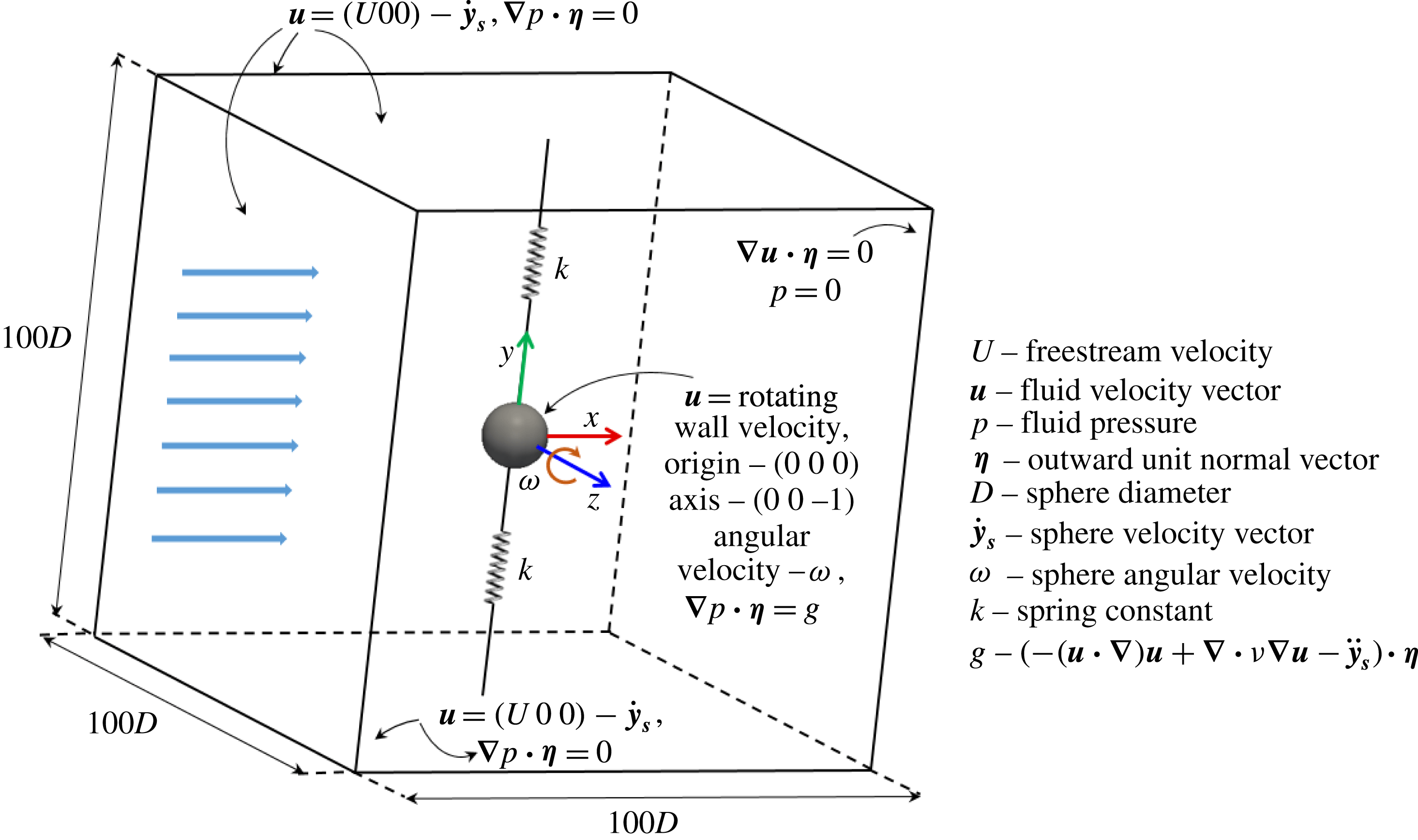
A uniform flow past a sphere forced to rotate and mounted with elastic supports in the transverse direction was investigated using the FSI solver. As shown in figure 1, the flow is in the
 $x$
direction, and the sphere is restricted to translate only in the
 $y$
direction while it rotates about the
 $-z$
direction with an angular velocity of
 $\unicode[STIX]{x1D714}$
. A cube of
 $100D$
was chosen for the fluid domain with the sphere at its centre. In this study, the sphere is assumed to translate as a spring–mass system without any damping to obtain the highest vibration amplitude. Moreover, in the FSI solver,
 $\boldsymbol{y}_{\boldsymbol{s}}$
,
 $\dot{\boldsymbol{y}}_{\boldsymbol{s}}$
,
 $\ddot{\boldsymbol{y}}_{\boldsymbol{s}}$
and
 $\boldsymbol{f}_{\boldsymbol{l}}$
are treated as vectors with zero
 $x$
and
 $z$
components, since the sphere translation is restricted to the
 $y$
direction only. At the inlet boundaries, a Dirichlet boundary condition was prescribed for the velocity, while a zero-gradient Neumann boundary condition was prescribed for the pressure, as shown in figure 1. At the sphere surface, no-slip and no-penetration boundary conditions were applied using a rotating wall velocity. A Neumann boundary condition was prescribed for the pressure at the sphere surface. However, the normal pressure gradient at the sphere surface is in general non-zero due to the rotation of the sphere. Therefore, it was calculated by taking the inner product of momentum equation (2.1) and the outward unit normal vector,
 $\boldsymbol{\unicode[STIX]{x1D702}}$
, as follows:
 $$\begin{eqnarray}\unicode[STIX]{x1D735}p\boldsymbol{\cdot }\boldsymbol{\unicode[STIX]{x1D702}}=(-(\boldsymbol{u}\boldsymbol{\cdot }\unicode[STIX]{x1D735})\boldsymbol{u}+\unicode[STIX]{x1D735}\boldsymbol{\cdot }\unicode[STIX]{x1D708}\unicode[STIX]{x1D735}\boldsymbol{u}-\ddot{\boldsymbol{y}}_{\boldsymbol{s}})\boldsymbol{\cdot }\boldsymbol{\unicode[STIX]{x1D702}}.\end{eqnarray}$$
At the outlet boundary, the pressure was set to zero while the velocity was prescribed as zero gradient in the normal direction.
Schematic of the computational domain and boundary conditions.

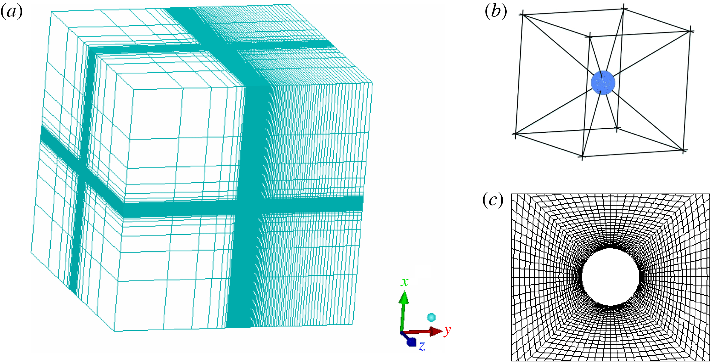
The unstructured-grid computational domain: (a) isometric view; (b) the cubic block placed around the sphere, which was decomposed into six square frustums; (c) grid near the sphere surface at
 $xy$
plane.

Figure 2 displays the unstructured grid used for the fluid domain. To achieve high concentration near the sphere, a cube of
 $5D$
was placed around the sphere. This cube was decomposed into six square frustum-shaped blocks, as shown in figure 2(b). The grid was compressed near the sphere surface by selecting an exponentially distributed cell thickness in the radial direction in each square frustum (see figure 2
c). A large number of grid points was assigned in the downstream direction to resolve the wake structures. Four finer grids were generated to assess the grid independence analysis (refer to the next section for more details). To optimise the grid generation process, initially, the number of cells on the surface of the sphere,
 $N$
, was kept constant at
 $7350$
. This grid (grid
 $1$
) comprised
 $\simeq 0.79$
million cells with a minimum cell thickness in the radial direction from the sphere surface,
 $\unicode[STIX]{x1D6FF}l$
, of
 $0.011D$
. The second grid was generated by decreasing
 $\unicode[STIX]{x1D6FF}l$
to
 $0.004D$
. This yielded
 $\simeq 1.25$
million cells, with approximately
 $10$
–
 $16$
cells within the boundary layer. This grid is sufficient to resolve the flow in the near wake. However, two more grids were generated to ensure that the solution was grid independent. In the third grid,
 $\unicode[STIX]{x1D6FF}l$
was further decreased to
 $0.002D$
by choosing the same number of cells as grid
 $2$
. Finally, the fourth grid was generated by increasing
 $N$
to
 $18\,150$
by choosing the same
 $\unicode[STIX]{x1D6FF}l$
as grid
 $2$
to observe the effect of cell thickness in the tangential direction on the solution. The non-dimensional time step,
 $\unicode[STIX]{x1D6FF}\unicode[STIX]{x1D70F}=\unicode[STIX]{x1D6FF}tU/D$
, used with each grid for all the analyses was
 $0.005$
.
3 Numerical sensitivity and validation studies
This section presents two validation studies. The first study aims to display the ability of capturing important physics of the flow past a rigidly mounted and transversely rotating sphere at Reynolds number
 $300$
. The second study demonstrates the validation of the newly built FSI solver for vortex-induced vibration studies. Finally, grid independence analyses performed for vortex-induced vibration of a sphere are presented.
3.1 Transversely rotating rigid sphere
Flow past a rigidly mounted and transversely rotating (in the
 $-z$
direction) sphere was investigated at
 $Re=300$
for the rotation rates
 $0\leqslant \unicode[STIX]{x1D6FC}\leqslant 3$
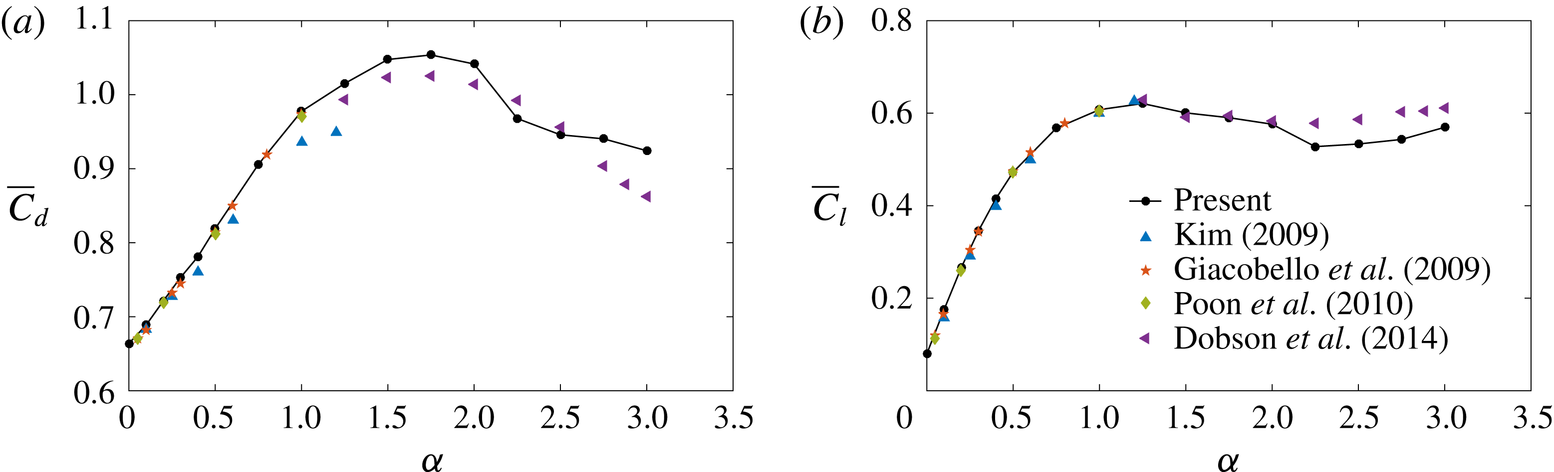
. The computed values of the time-mean drag coefficient,
 $\overline{C}_{d}$
, and the time-mean lift coefficient,
 $\overline{C_{l}}$
, are compared with other studies in figures 3(a) and 3(b), respectively. The present results agree well with the results in the literature (Giacobello et al.
Reference Giacobello, Ooi and Balachandar2009; Kim Reference Kim2009; Poon et al.
Reference Poon, Ooi, Giacobello and Cohen2010; Dobson et al.
Reference Dobson, Ooi and Poon2014). The time-mean lift coefficient increased with increasing
 $\unicode[STIX]{x1D6FC}$
but levelled off at higher rotation rates. The drag coefficient increased with
 $\unicode[STIX]{x1D6FC}$
up to
 $\unicode[STIX]{x1D6FC}\approx 1.75$
and then decreased.
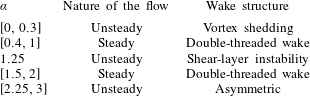
The flow underwent a series of transitions between ‘steadiness’ and ‘unsteadiness’ as the rotation rate increased from
 $0$
, as shown in table 1. From
 $\unicode[STIX]{x1D6FC}=0$
to
 $0.3$
, the flow was unsteady with vortex shedding. Moreover, the shedding frequency increased as the rotation rate increased. For
 $\unicode[STIX]{x1D6FC}=0.4$
, the flow became steady with a double-threaded wake structure. As
 $\unicode[STIX]{x1D6FC}$
increased further, the flow remained steady until
 $\unicode[STIX]{x1D6FC}=2$
with a double-threaded wake, except for
 $\unicode[STIX]{x1D6FC}=1.25$
, where the flow was unstable due to the shear-layer instability, as discussed by Kim (Reference Kim2009). For
 $\unicode[STIX]{x1D6FC}\in [2.25,3]$
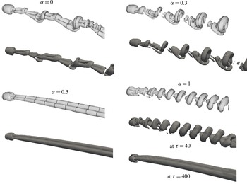
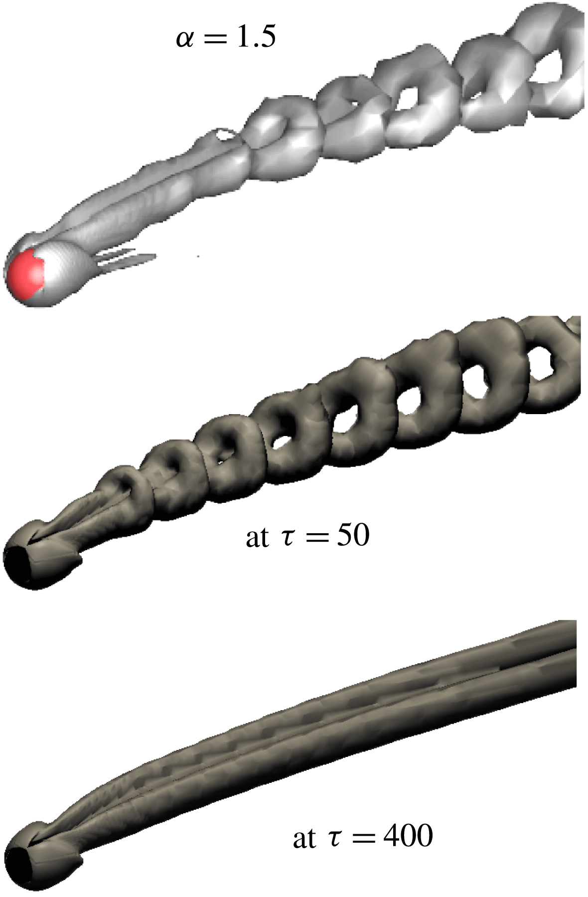
, the flow became unstable again, but with an asymmetric wake structure having no symmetry at all. Figures 4 and 5 show comparisons of wake structures observed in the present study with Giacobello et al. (Reference Giacobello, Ooi and Balachandar2009) and Dobson et al. (Reference Dobson, Ooi and Poon2014) at five rotation rates. The wake structures observed at low rotation rates (
 $\unicode[STIX]{x1D6FC}\in [0,0.6]$
) match well with other research studies; for example, for
 $\unicode[STIX]{x1D6FC}=0$
,
 $0.3$
and
 $0.5$
. At higher rotation rates, for example, for
 $\unicode[STIX]{x1D6FC}=1$
and
 $1.5$
, the wake structures observed at the initial stage are similar to those observed by Giacobello et al. (Reference Giacobello, Ooi and Balachandar2009) and Dobson et al. (Reference Dobson, Ooi and Poon2014). However, for very long simulation times, the initially unsteady flow became steady with a double-threaded wake structure.
Comparison with other numerical studies of computed time-mean drag coefficient,
 $\overline{C}_{d}$
, and time-mean lift coefficient,
 $\overline{C_{l}}$
, for flow past a rigidly mounted and transversely rotating sphere at
 $Re=300$
for
 $0\leqslant \unicode[STIX]{x1D6FC}\leqslant 3$
.

Comparison of the nature of the flow with the rotation rate of flow past a transversely rotating sphere.

Wake structures of a rigidly mounted and transversely rotating sphere for
 $\unicode[STIX]{x1D6FC}=0$
,
 $0.3$
,
 $0.5$
and
 $1$
. Light grey structures are the results of Giacobello et al. (Reference Giacobello, Ooi and Balachandar2009); dark structures are the results of the present study identified using the method of Jeong & Hussain (Reference Jeong and Hussain1995) at
 $\unicode[STIX]{x1D706}_{2}=-5\times 10^{-4}$
. For
 $\unicode[STIX]{x1D6FC}=1$
, the wake structure varied with the time. Initially, the flow was unsteady as shown at
 $\unicode[STIX]{x1D70F}=40$
, but for longer simulation time, the flow became stable with a double-threaded wake structure, as shown at
 $\unicode[STIX]{x1D70F}=400$
, where
 $\unicode[STIX]{x1D70F}=tU/D$
is the non-dimensional time.

Comparison of wake structures of a rigidly mounted and transversely rotating sphere for
 $\unicode[STIX]{x1D6FC}=1.5$
with Dobson et al. (Reference Dobson, Ooi and Poon2014) (the dark structure). The light structures are the results of the present study.

3.2 Validation: VIV of a cylinder
A series of simulations was conducted with a rigidly mounted cylinder (non-rotating) to validate the numerical solver developed for the FSI problems by selecting the study by Leontini, Thompson & Hourigan (Reference Leontini, Thompson and Hourigan2006b
) as the base case. The mass ratio, damping constant and the Reynolds number of the flow were fixed at
 $m^{\ast }=10$
,
 $\unicode[STIX]{x1D701}=0.01$
and
 $Re=200$
, respectively, while varying the reduced velocity from
 $U^{\ast }=3.5$
to
 $7.1$
. The oscillation amplitude of the cylinder,
 $A^{\ast }$
, the fluctuation amplitude of the lift coefficient,
 $C_{l}^{\prime }$
, the frequency ratio of cylinder vibration to the natural frequency of the system,
 $f^{\ast }=f/f_{n}$
, and the average phase angle between lift force and cylinder vibration,
 $\unicode[STIX]{x1D719}$
, were calculated and compared with Leontini et al. (Reference Leontini, Thompson and Hourigan2006b
). The percentage difference calculated for
 $A^{\ast }$
,
 $C_{l}^{\prime }$
,
 $f^{\ast }$
, and
 $\unicode[STIX]{x1D719}$
are
 $-8\,\%$
,
 $-8\,\%$
,
 $1.8\,\%$
and
 $3.6\,\%$
, respectively, compared to the results of Leontini et al. This study provides validation for the new solver.
3.3 Resolution studies
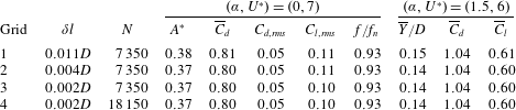
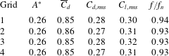
All FSI simulations reported in the next section have been carried out on grid 2. To verify that this grid is fine enough to resolve the flow for FSI simulations, two grid sensitivity analyses were performed; one analysis for the vibrating sphere cases for the parameters,
 $\unicode[STIX]{x1D6FC}=0$
and
 $U^{\ast }=7$
; a second analysis for the higher rotation rates for the parameters
 $\unicode[STIX]{x1D6FC}=1.5$
and
 $U^{\ast }=6$
. Both analyses were performed at
 $Re=300$
and
 $m^{\ast }=2.865$
(or
 $m_{r}=1.5$
). For the first analysis,
 $U^{\ast }=7$
was chosen because the sphere showed a maximum oscillation around this value. Table 2 compares the effect of grid refinement for both analyses. In the first analysis (
 $\unicode[STIX]{x1D6FC}=0$
and
 $U^{\ast }=7$
), the sphere underwent synchronised vibrations. Therefore, the results were tabulated for the sphere oscillation amplitude,
 $A^{\ast }$
, force coefficients (time-mean drag coefficient,
 $\overline{C}_{d}$
, root-mean-square (r.m.s.) values of the fluctuation components of drag and lift coefficients,
 $C_{d,rms}$
and
 $C_{l,rms}$
), and frequency ratio,
 $f^{\ast }=f/f_{n}$
. In the second analysis (
 $\unicode[STIX]{x1D6FC}=1.5$
and
 $U^{\ast }=6$
), the flow was steady and the sphere moved to a new position and remained with no vibration. Therefore, the time-mean sphere displacement,
 $\overline{Y}/D$
, time-mean drag and lift coefficients
 $\overline{C}_{d}$
, and
 $\overline{C}_{l}$
were calculated. It is noted that there is less than
 $1\,\%$
variation in the results between grid
 $1$
and grid
 $2$
for both analyses. The results obtained for grids
 $2$
–
 $4$
agree well with each other. Therefore, for the Reynolds number and rotation rate range of interest, decreasing
 $\unicode[STIX]{x1D6FF}l$
or increasing
 $N$
further has a negligible effect on the results. Thus, we can conclude that grid
 $2$
is sufficient for all VIV simulations at
 $Re=300$
, and therefore, this grid was used to obtain all subsequently presented results. As pointed out above, the non-dimensional time step used in these resolution studies and all the other simulations is
 $\unicode[STIX]{x1D6FF}\unicode[STIX]{x1D70F}=0.005$
. It was verified that reducing the time step by a factor of two, resulted in a less than 1 % change to the key convergence measures discussed above.
The sensitivity of the spatial resolution of the flow parameters of vortex-induced vibration of a rotating sphere at
 $(\unicode[STIX]{x1D6FC},U^{\ast })=(0,7)$
and
 $(1.5,6)$
,
 $Re=300$
and
 $m^{\ast }=2.865$
(
 $m_{r}=1.5$
).
 $\unicode[STIX]{x1D6FF}l$
is the minimum thickness of the cells (in the radial direction) at the sphere surface in each grid and
 $N$
is the number of cells on the sphere surface. The oscillation amplitude of the sphere,
 $A^{\ast }$
, the time-mean sphere displacement,
 $\overline{Y}/D$
, the time-mean drag and lift coefficients,
 $\overline{C}_{d}$
and
 $\overline{C}_{l}$
, the r.m.s. values of fluctuation component of the drag and lift coefficients,
 $C_{d,rms}$
and
 $C_{l,rms}$
, and the ratio of vortex-shedding frequency to the natural frequency,
 $f/f_{n}$
, are listed.

4 Effects of transverse rotation on VIV of a sphere
This section presents and discusses the results obtained for flow past an elastically mounted sphere (allowed to translate only in the
 $y$
direction) forced to rotate about the
 $-z$
direction at the Reynolds number
 $Re=300$
and the reduced mass
 $m_{r}=1.5$
(which is equivalent to the mass ratio
 $m^{\ast }=2.865$
) for rotation rates
 $0\leqslant \unicode[STIX]{x1D6FC}\leqslant 2.5$
and a reduced-velocity range
 $3.5\leqslant U^{\ast }\leqslant 11$
. Non-rotating VIV studies, especially the many studies of circular cylinders but also spheres, show that the amplitude response is not a very strong function of mass ratio, but rather a function of the mass-damping ratio (
 $m^{\ast }\unicode[STIX]{x1D701}$
), as discussed in the introduction. The choice of a relatively small mass ratio of
 $m^{\ast }\simeq 2.9$
was chosen to ensure a strong VIV response at the Reynolds number made for the first part of this study. While a significantly larger mass ratio may enable modes III and IV to be investigated, this would increase the computational cost significantly, because a sphere with much higher inertia requires considerably more time to reach an asymptotic oscillatory state. The chosen mass ratio is slightly lower than used by Behara et al. (Reference Behara, Borazjani and Sotiropoulos2011) of
 $m_{r}=2$
for their 3-DOF non-rotating sphere VIV studies; however, comparisons of current results with theirs for the same setup (3-DOF VIV) and parameters (
 $Re=300$
,
 $m_{r}=2$
), show a comparable amplitude response curve, and also confirm the relative insensitivity to mass ratio, as discussed in Rajamuni et al. (Reference Rajamuni, Thompson and Hourigan2018).
The non-dimensional rotation rate,
 $\unicode[STIX]{x1D6FC}$
, was prescribed through setting the angular velocity of the sphere,
 $\unicode[STIX]{x1D714}$
, so that (
 $\unicode[STIX]{x1D6FC}=\unicode[STIX]{x1D714}D/(2U)$
). This prescribed the velocity boundary condition on the sphere surface, while the reduced velocity was prescribed through setting the spring constant in the solid motion equation by
 $k=4m\unicode[STIX]{x03C0}^{2}/U^{\ast 2}$
.
The results are presented in the following three subsections. Initially, the sphere response is discussed with its time-mean position, oscillation amplitude and the frequency of oscillation. Then, the forces exerted on the sphere are given in terms of time-mean values and fluctuation amplitudes. Finally, the behaviour of the flow is analysed through the wake structures observed behind the sphere.
4.1 Sphere response
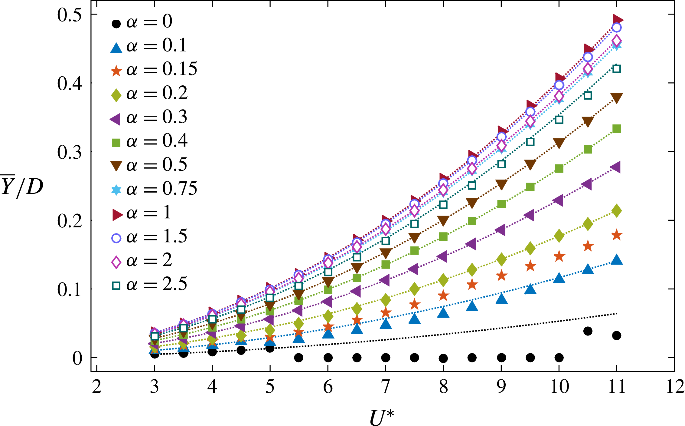
Figure 6 shows the variation of time-mean position of the sphere,
 $\overline{Y}/D$
, with the reduced velocity at each rotation rate, where
 $Y=\boldsymbol{y}_{\boldsymbol{s}}\boldsymbol{\cdot }(0\;1\;0)$
is the displacement of the sphere in the
 $y$
direction. As can be seen,
 $\overline{Y}$
increased monotonically with increasing reduced velocity for each
 $\unicode[STIX]{x1D6FC}$
, except
 $\unicode[STIX]{x1D6FC}=0$
. This is because of the lower effective stiffness of springs at higher reduced velocities. At each reduced velocity, the time-mean position of the sphere,
 $\overline{Y}$
, increased with the rotation rate up to
 $\unicode[STIX]{x1D6FC}=1$
, as expected from the Magnus force applied on the sphere, and this was more prominent as the reduced velocity increased. However, as
 $\unicode[STIX]{x1D6FC}$
increased from
 $1$
to
 $2.5$
,
 $\overline{Y}$
did not increase further; instead it slightly decreased (see the curves with hollow symbols for
 $\unicode[STIX]{x1D6FC}=1.5$
,
 $2$
and
 $2.5$
in figure 6). At a fixed reduced velocity, the variation of
 $\overline{Y}$
with
 $\unicode[STIX]{x1D6FC}$
agrees well with the trend of the lift coefficient calculated for the transversely rotating and rigidly mounted sphere (see figure 3
b). The time-mean position of the sphere can be estimated as
 $\overline{Y}/D=3\overline{C}_{l}U^{\ast 2}/(16m^{\ast }\unicode[STIX]{x03C0}^{2})$
from the time-mean lift coefficient,
 $\overline{C}_{l}$
, calculated for the transversely rotating and rigidly mounted sphere at each
 $\unicode[STIX]{x1D6FC}$
by considering the time-mean form of the solid motion equation (2.3). The dotted lines in figure 6 represent the estimated
 $\overline{Y}/D$
at each
 $\unicode[STIX]{x1D6FC}$
. However, the actual values of
 $\overline{Y}/D$
slightly differ from the estimated values for some ranges of
 $U^{\ast }$
at some rotation rates, especially for
 $\unicode[STIX]{x1D6FC}=0$
. The reason for this deviation is explained later in § 4.2.
Variation of the time-mean position of the sphere,
 $\overline{Y}/D$
, with the reduced velocity,
 $U^{\ast }$
, at each rotation rate: the dotted lines represent the estimated time-mean position of the sphere according to the time-mean lift force,
 $\overline{C}_{l}$
, calculated for a rigidly mounted sphere at each rotation rate (
 $\overline{Y}/D=3\overline{C}_{l}U^{\ast 2}/(16m^{\ast }\unicode[STIX]{x03C0}^{2})$
).

The sphere response: (a) the variation of the maximum oscillation amplitude,
 $A^{\ast }$
, with the reduced velocity,
 $U^{\ast }$
, at each rotation rate; and (b) the frequency ratio
 $f^{\ast }=f/f_{n}$
for rotation rates and reduced velocities at which the sphere showed a vibrational response.

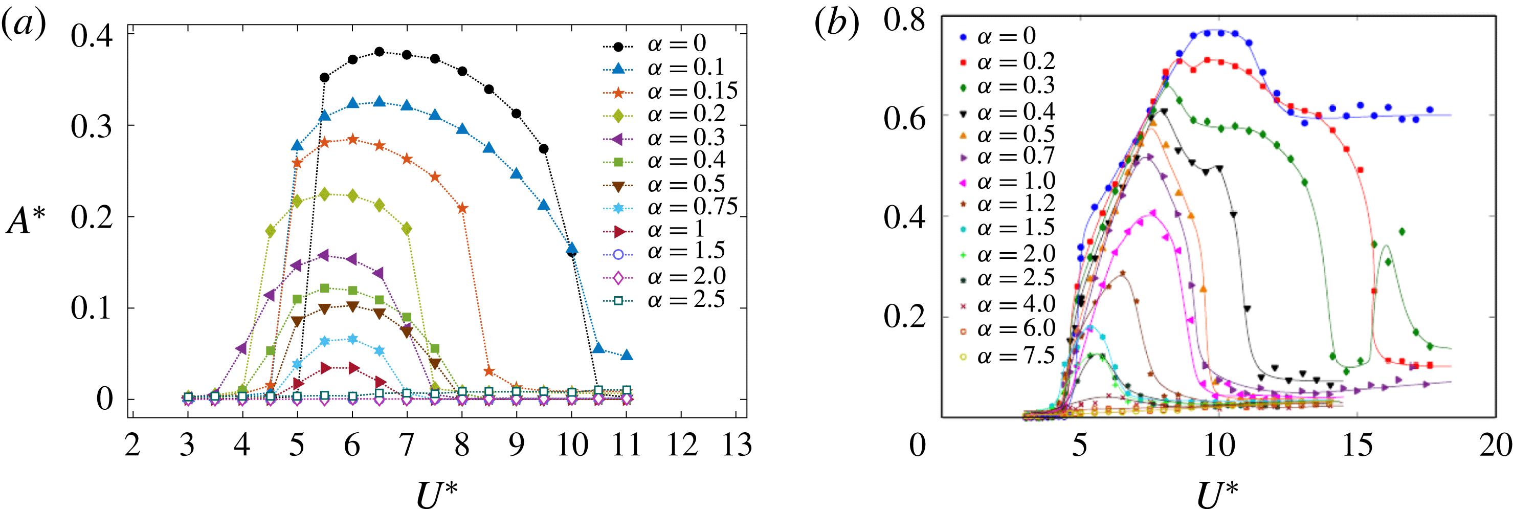
Figure 7 displays the effects of transverse rotation on the characteristics of the vortex-induced vibration of a sphere with the oscillation amplitude,
 $A^{\ast }=\sqrt{2}Y_{rms}/D$
, and the frequency ratio,
 $f^{\ast }=f/f_{n}$
, over the reduced-velocity range
 $3.5\leqslant U^{\ast }\leqslant 11$
for
 $\unicode[STIX]{x1D6FC}=0$
–
 $2.5$
, where
 $f$
is the frequency of the sphere vibration and
 $f_{n}$
is the mechanical natural frequency of the system in the medium without the added-mass contribution. For the non-rotating case (
 $\unicode[STIX]{x1D6FC}=0$
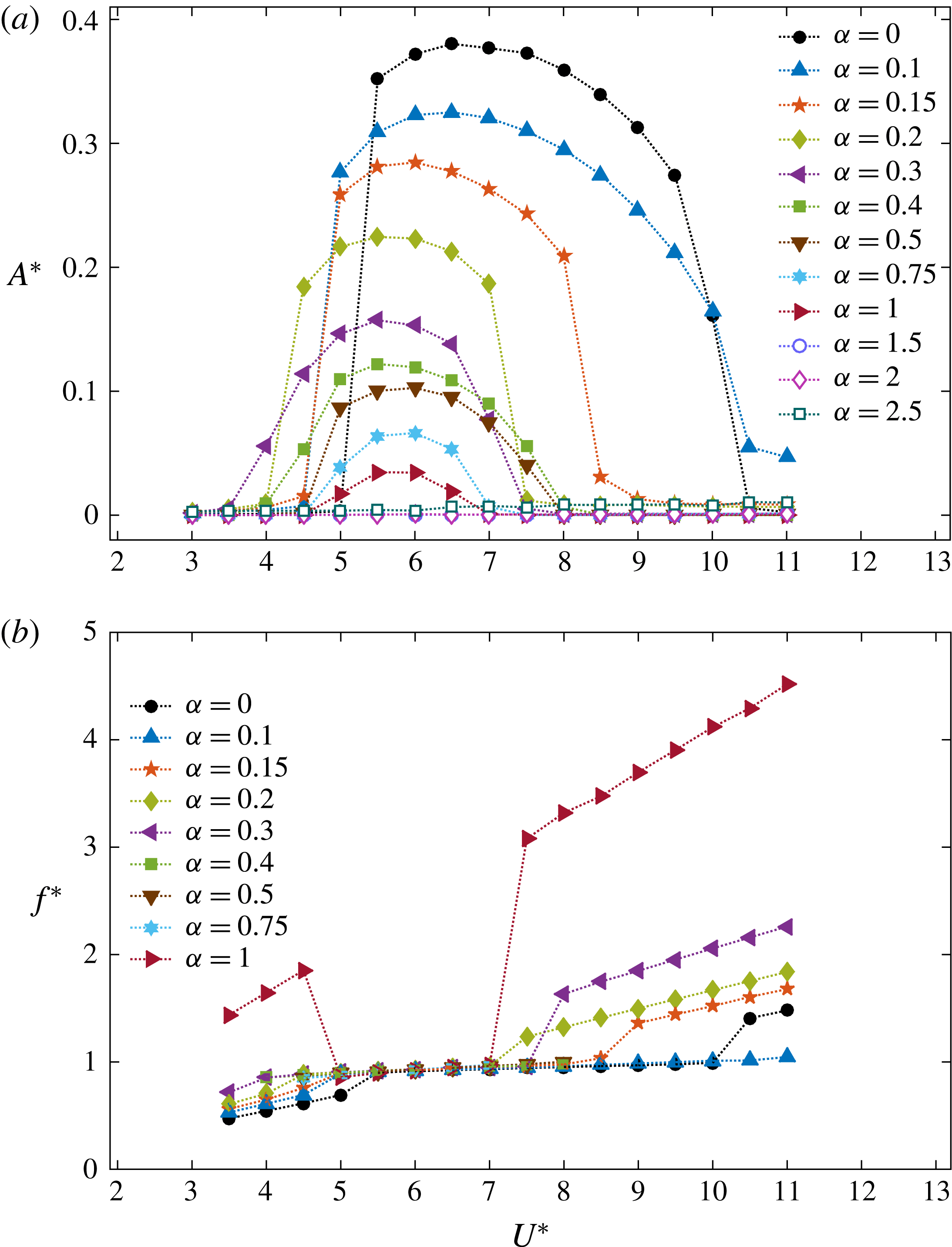
), the sphere showed a relatively large oscillation amplitude (
 $A^{\ast }\simeq 0.4D$
) from
 $U^{\ast }=5.5$
to
 $10$
(see the curve with black dots in figure 7
a). In this case, at these reduced velocities, the time-mean position of the sphere deviated from the estimated values calculated with the lift force of a rigidly mounted sphere, and remained at its initial position (
 $\overline{Y}=0$
for
 $\unicode[STIX]{x1D6FC}=0$
and
 $U^{\ast }\in [5.5,10]$
, see figure 6). Thus, those oscillations were symmetric through the initial position of the sphere. Furthermore, as can been seen from figure 7(b), at those reduced velocities, the frequencies of the sphere displacement and vortex shedding were synchronised and close to the natural frequency of the system (
 $f^{\ast }\simeq 1$
), indicating that these are vortex-induced vibration responses.
For
 $\unicode[STIX]{x1D6FC}=0$
, the sphere began to show large amplitude vibrations suddenly as the reduced velocity increased from
 $5$
to
 $5.5$
. A similar observation was reported by Behara et al. (Reference Behara, Borazjani and Sotiropoulos2011) and Behara & Sotiropoulos (Reference Behara and Sotiropoulos2016) in their studies on the vortex-induced vibration of a sphere with 3 DOF. The shape of the response curve for
 $\unicode[STIX]{x1D6FC}=0$
strongly resembles the response curves that they observed. In addition, the response curve for
 $\unicode[STIX]{x1D6FC}=0$
shows similarities to modes I and II vibration observed by experimental studies on tethered spheres by Govardhan & Williamson (Reference Govardhan and Williamson1997), Jauvtis et al. (Reference Jauvtis, Govardhan and Williamson2001) and Govardhan & Williamson (Reference Govardhan and Williamson2005). This will be further discussed in the force measurements section.
Interestingly, the sphere response was modified greatly when subjected to a forced rotation. Similar to the non-rotating case, significant vibrations were observed for the rotating cases up to the rotation rate
 $\unicode[STIX]{x1D6FC}=1$
. Importantly, the response amplitude decreased with the increasing rotation rate up to
 $\unicode[STIX]{x1D6FC}=1$
, and it was suppressed for
 $\unicode[STIX]{x1D6FC}\geqslant 1.5$
, as shown in figure 7(a). Figure 7(b) shows that for all the cases for which the sphere vibrated significantly, the vibration frequency was locked in to the vortex-shedding frequency and was close to the system’s natural frequency; this again confirms that all of these responses are vortex-induced vibration responses.
Variation of the oscillation amplitude,
 $A^{\ast }$
, and the time-mean position,
 $\overline{Y}/D$
, of the sphere with the rotation rate,
 $\unicode[STIX]{x1D6FC},$
at the reduced velocity
 $U^{\ast }=6$
.

Variations of (a) the maximum oscillation amplitude of the sphere,
 $A_{max}^{\ast }$
, and (b) the reduced velocity at which the sphere showed a maximum oscillation amplitude with the rotation rate,
 $\unicode[STIX]{x1D6FC}$
.

The sphere response was further investigated in the range,
 $\unicode[STIX]{x1D6FC}=[1,1.5]$
at the reduced velocity,
 $U^{\ast }=6$
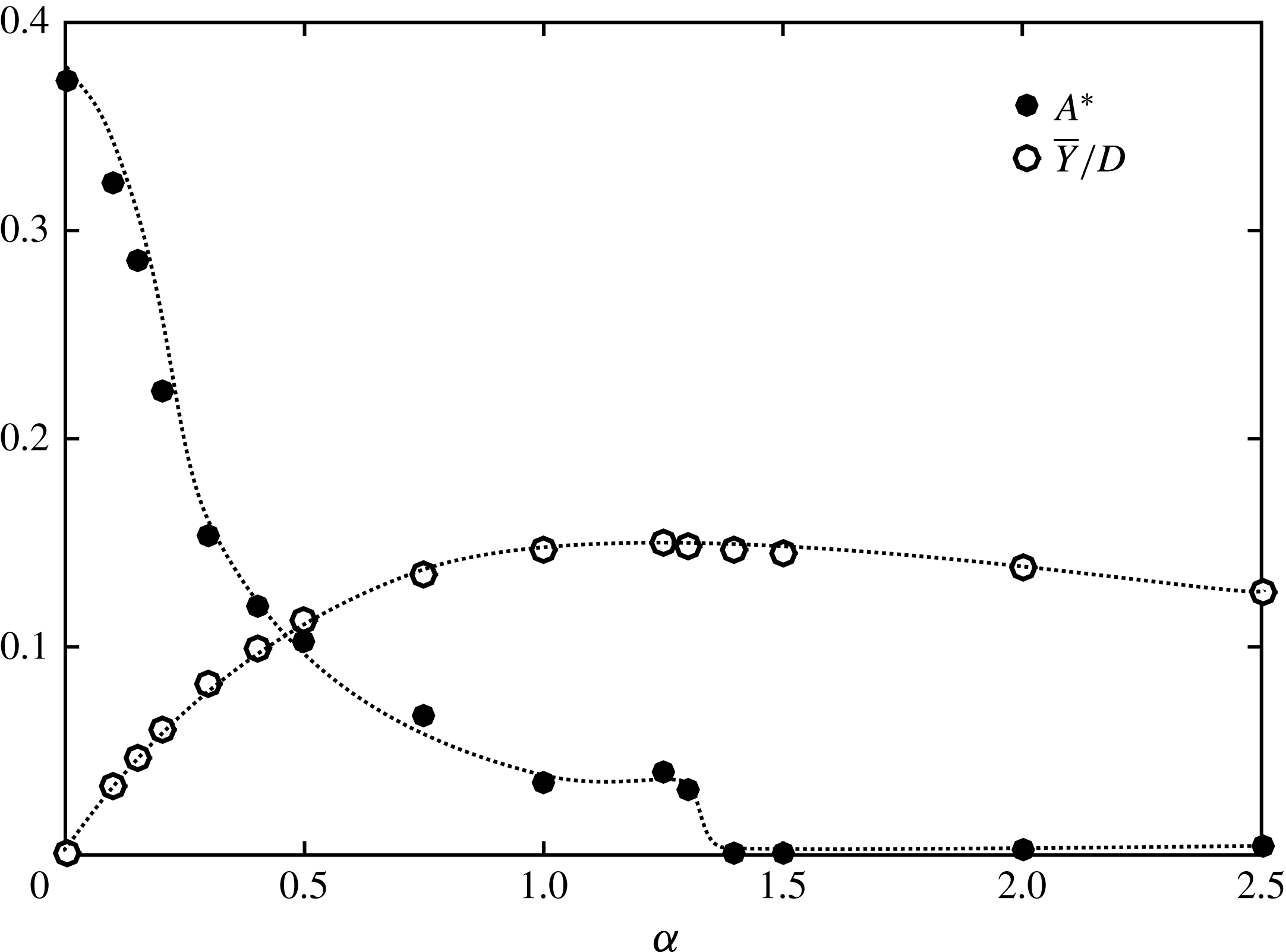
which is close to the maximum response. As can be seen from figure 8, the sphere showed synchronised vibrations up to
 $\unicode[STIX]{x1D6FC}=1.3$
. The sphere response amplitude decreased rapidly for small
 $\unicode[STIX]{x1D6FC}$
but was nearly flat in the range,
 $\unicode[STIX]{x1D6FC}\in [1,1.3]$
and VIV was completely suppressed for
 $\unicode[STIX]{x1D6FC}>1.4$
. The time-mean position of the sphere,
 $\overline{Y}/D$
, shifted away from its initial position with increasing rotation rate up to
 $\unicode[STIX]{x1D6FC}=1.3$
, and for
 $\unicode[STIX]{x1D6FC}\geqslant 1.4$
the time-mean position of the sphere returned back towards the initial position of the sphere for increasing
 $\unicode[STIX]{x1D6FC}$
. The cutoff
 $\unicode[STIX]{x1D6FC}$
for the occurrence of VIV is likely to depend on the Reynolds number, so this cutoff was not further refined over a range of
 $U^{\ast }$
.
The amplitude responses appear as approximately bell-shaped curves for each
 $\unicode[STIX]{x1D6FC}$
for
 $\unicode[STIX]{x1D6FC}\leqslant 1$
(see figure 7
a). Similar to the non-rotating case, the synchronised vibrations began suddenly for
 $\unicode[STIX]{x1D6FC}\leqslant 0.2$
. Moreover, the synchronised vibrations ended suddenly for
 $\unicode[STIX]{x1D6FC}=0.15$
and
 $0.2$
. In contrast to lower rotation rates, for higher rotation rates (
 $\unicode[STIX]{x1D6FC}\geqslant 0.3$
), the synchronised vibrations appeared and disappeared more gradually at both ends of the synchronised
 $U^{\ast }$
range. The synchronisation regime, which is the reduced-velocity range over which the sphere showed synchronised vibrations, varied with rotation rate. For
 $\unicode[STIX]{x1D6FC}=0.1$
, the synchronisation regime widened to
 $U^{\ast }=5$
–
 $11$
. However, it generally narrowed as
 $\unicode[STIX]{x1D6FC}$
increased from
 $0.1$
, and yielded a narrow synchronisation regime of
 $U^{\ast }=5$
–
 $6.5$
for
 $\unicode[STIX]{x1D6FC}=1$
. In addition, the synchronisation regime mostly shifted to the left (to lower reduced velocities) as the rotation rate increased.
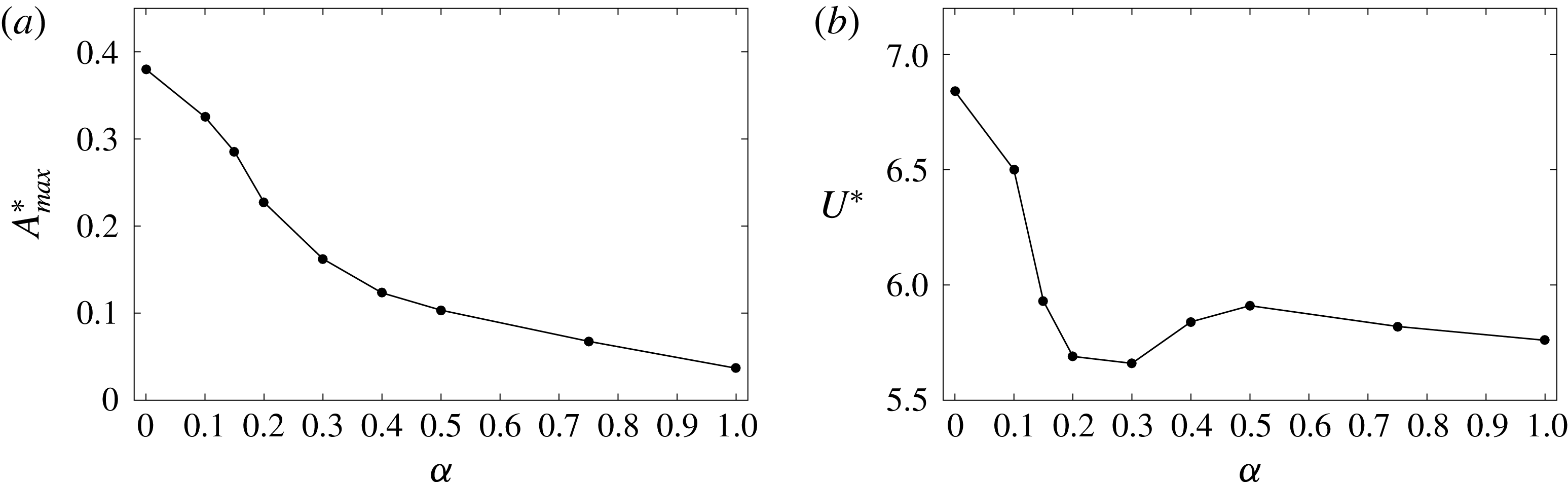
Panels 9(a) and 9(b) show the variation of the maximum oscillation amplitude of the sphere,
 $A_{max}^{\ast }$
, and of the reduced velocity,
 $U^{\ast }$
, at which the maximum oscillation amplitude was observed with the rotation rate, respectively. As can be seen, the maximum oscillation amplitude decreased gradually with increasing rotation rate. The reduced velocity at which the sphere showed a maximum oscillation amplitude shifted to lower values as
 $\unicode[STIX]{x1D6FC}$
increased from
 $0$
to
 $0.3$
. However, it increased and then decreased, as
 $\unicode[STIX]{x1D6FC}$
increased from
 $0.3$
to
 $1$
(see figure 9
b).
Time history of the sphere response (a) for
 $\unicode[STIX]{x1D6FC}=0.15$
and
 $U^{\ast }=3.5$
,
 $5$
,
 $7.5$
,
 $8.5$
and
 $9.5$
; (b) for
 $\unicode[STIX]{x1D6FC}=0.5$
and
 $U^{\ast }=3.5$
,
 $5$
,
 $6$
,
 $7.5$
and
 $10$
.

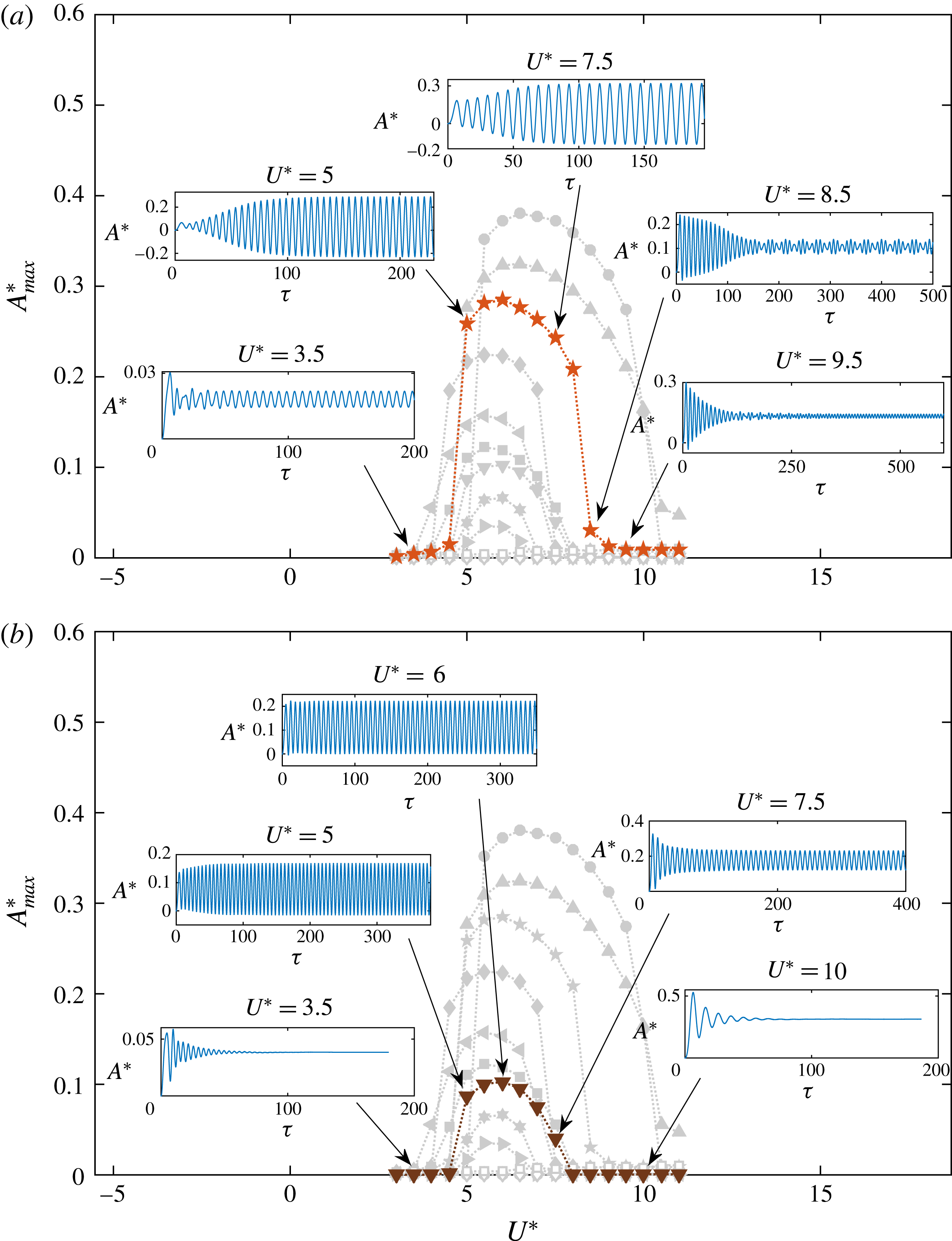
The time history of the sphere displacement is shown in figure 10(a) for
 $\unicode[STIX]{x1D6FC}=0.15$
and in figure 10(b) for
 $\unicode[STIX]{x1D6FC}=0.5$
, for five different reduced velocities. At each rotation rate, the sphere vibrated (approximately) sinusoidally in the asymptotic state when in the synchronisation regime. Beyond the synchronisation regime at higher reduced velocities, the sphere initially vibrated significantly, but later, the vibration amplitude decreased substantially (see the time history at
 $U^{\ast }=8.5$
and
 $9.5$
in figure 10
a). Moreover, in some cases, the sphere response just beyond the synchronisation regime consisted of two frequencies, as shown in figure 10(a) for
 $\unicode[STIX]{x1D6FC}=0.15$
and
 $U^{\ast }=8.5$
. In this case, the dominant frequency is the natural frequency of the system and the secondary frequency corresponds to the vortex-shedding frequency.
For
 $\unicode[STIX]{x1D6FC}\leqslant 0.3$
, small-scale vibrations were observed outside the synchronisation regimes, as shown in figure 10(a) for
 $\unicode[STIX]{x1D6FC}=0.15$
. Interestingly, for
 $\unicode[STIX]{x1D6FC}=0.4$
,
 $0.5$
and
 $0.75$
, the vibrations were suppressed outside the synchronisation regime, as shown in figure 10(b) for
 $\unicode[STIX]{x1D6FC}=0.5$
. However, for
 $\unicode[STIX]{x1D6FC}=1$
, outside the synchronisation regime, the sphere vibrated with a very small amplitude (
 $\ll 0.001D$
) and a high frequency (see figure 7
b). In this case, the wake frequency for a non-VIV rotating sphere is approximately a factor of three higher than at lower rotation rates, because the rapid rotation leads to a shear-layer shedding mode. The sphere responses were flat without any oscillations in the steady state for
 $\unicode[STIX]{x1D6FC}=1.5$
and
 $2$
for all the reduced velocities considered. However, for
 $\unicode[STIX]{x1D6FC}=2.5$
, the sphere oscillated with a small amplitude for all the reduced velocities. As discussed in § 3.1, when the sphere is rigidly mounted and with a forced transverse rotation, the flow was unsteady with vortex shedding behind the sphere for
 $\unicode[STIX]{x1D6FC}\leqslant 0.3$
; was steady for
 $0.4\leqslant \unicode[STIX]{x1D6FC}\leqslant 2$
, and was unsteady with an irregular wake for
 $\unicode[STIX]{x1D6FC}=2.5$
. Therefore, our observation of the sphere response outside the synchronisation regimes for
 $\unicode[STIX]{x1D6FC}\leqslant 0.75$
, and the sphere response for
 $\unicode[STIX]{x1D6FC}\geqslant 1.4$
are consistent with the observation of flow past a rigidly mounted and transversely rotating sphere.
As can be seen from figure 7(b), for the cases where the sphere showed small-scale vibrations outside the synchronisation regime (
 $\unicode[STIX]{x1D6FC}=0$
,
 $0.1$
,
 $0.15$
,
 $0.2$
,
 $0.3$
and
 $1$
), the vibration frequency of the sphere linearly increased with the reduced velocity. Moreover, the frequency increased with increasing rotation rate. This is consistent with the observation of an increasing vortex-shedding frequency with the rotation rate when the flow is unsteady for a rigidly mounted sphere (Kim Reference Kim2009).
Bourguet & Jacono (Reference Bourguet and Jacono2014) studied the effects of transverse rotation on flow-induced vibration of a cylinder at
 $Re=100$
for the rotation rates
 $\unicode[STIX]{x1D6FC}\in [0,4]$
in the reduced-velocity range
 $0\leqslant U^{\ast }\leqslant 32$
. They observed that when the cylinder was subjected to a forced rotation, it moved to a new position and showed synchronised vibration through this new position for a range of reduced velocities, similar to our observation with a rotating sphere. However, contrary to the decrease in the vibration amplitude we observed for a sphere, they observed an increase in the vibration amplitude for a cylinder with increasing rotation rate, which is also seen in much higher Reynolds number experiments (Wong et al.
Reference Wong, Zhao, Lo Jacono, Thompson and Sheridan2017). Moreover, for a rotating cylinder, the synchronisation regime expanded for higher reduced velocities up to
 $\unicode[STIX]{x1D6FC}=3.5$
, and then narrowed, whereas for a rotating sphere it was wider for
 $\unicode[STIX]{x1D6FC}=0.1$
and then mostly narrowed as
 $\unicode[STIX]{x1D6FC}$
increased. Interestingly, synchronised vibrations were suppressed for higher rotation rates for both the sphere (for
 $\unicode[STIX]{x1D6FC}>1.3$
) and the cylinder (for
 $\unicode[STIX]{x1D6FC}=4$
).
The variation sphere response amplitude with reduced velocity at each rotation rate: (a) present results of this numerical study at
 $Re=300$
, (b) results of the experimental study of Sareen et al. (Reference Sareen, Zhao, Lo Jacono, Sheridan, Hourigan and Thompson2018) over the Reynolds number range,
 $Re=5000$
–
 $30\,000$
.

More recently, Sareen et al. (Reference Sareen, Zhao, Lo Jacono, Sheridan, Hourigan and Thompson2018) investigated the effect of transverse rotation on vortex-induced vibration of a sphere experimentally. They varied the rotation rate over
 $\unicode[STIX]{x1D6FC}\in [0,7.5]$
and the reduced velocity over
 $U^{\ast }\in [3,18]$
, which corresponds to the Reynolds number range,
 $Re\in [5000,30\,000]$
. Figure 11 compares our observations of the sphere response amplitude with their observations. Despite the significant difference in Reynolds number, consistent with our predictions, they observed a decrease in the maximum sphere response amplitude and a narrowing of the synchronisation regime as the rotation rate increased. However, vortex-induced vibration persisted until
 $\unicode[STIX]{x1D6FC}=4$
at the higher Reynolds numbers. At the lower Reynolds number (
 $Re=300$
), the highest rotation rate that showed synchronised vibration was
 $\unicode[STIX]{x1D6FC}=1.3$
.
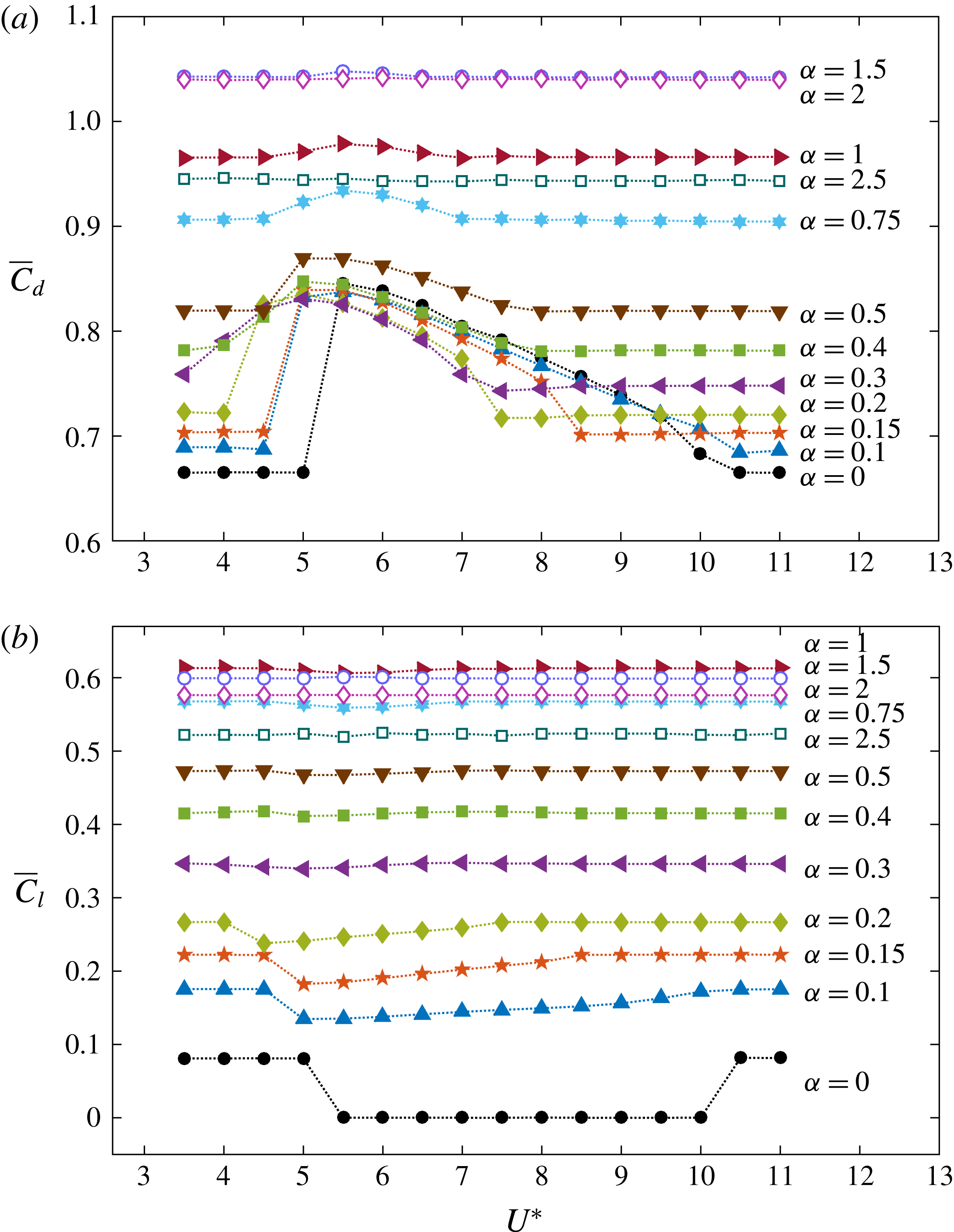
Variation of the time-mean (a) drag force coefficient,
 $\overline{C}_{d}$
, and (b) lift force coefficient in the
 $y$
direction,
 $\overline{C}_{ly}$
, with the reduced velocity,
 $U^{\ast }$
, at each rotation rate.

4.2 Force measurements
Figure 12 shows plots of the variation of the time-mean drag and lift coefficients,
 $\overline{C}_{d}$
and
 $\overline{C}_{l}$
, respectively, as functions of the reduced velocity at each rotation rate. The lift coefficient in the
 $z$
direction was negligible compared to the lift coefficient in the
 $y$
direction,
 $C_{ly}$
, for all the cases except
 $\unicode[STIX]{x1D6FC}=0$
and
 $U^{\ast }\in [10.5,11]$
. Therefore,
 $\overline{C}_{l}=\overline{C}_{ly}$
except for
 $\unicode[STIX]{x1D6FC}=0$
and
 $U^{\ast }\in [10.5,11]$
. Outside the synchronisation regimes, both
 $\overline{C}_{d}$
and
 $\overline{C}_{l}$
were constant, having the values calculated for a rigidly mounted sphere at each
 $\unicode[STIX]{x1D6FC}$
. However, both
 $\overline{C}_{d}$
and
 $\overline{C}_{l}$
varied significantly from the values for a rigidly mounted sphere at the reduced velocities for which the sphere showed synchronised vibrations. This is consistent with the fact that the time-mean sphere displacement differed from the estimated values based on the lift force of a rigidly mounted rotating sphere in the synchronisation regimes as shown in figure 6 (see § 4.1). At a given reduced velocity, the lift force increased with increasing rotation rate up to
 $\unicode[STIX]{x1D6FC}=1$
, and then decreased, similar to the variation of
 $\overline{Y}/D$
with
 $\unicode[STIX]{x1D6FC}$
.
For the non-rotating case (
 $\unicode[STIX]{x1D6FC}=0$
), the time-mean lift coefficient dropped down to zero during the synchronisation regime (see the curve with black dots in figure 12
b). This is consistent with the synchronised vibrations of the sphere being symmetric about the initial position of the sphere for
 $\unicode[STIX]{x1D6FC}=0$
. For the rotating cases, in the synchronisation regimes,
 $\overline{C}_{l}$
decreased from the non-oscillatory value, and the decrement reduced, with the increasing
 $\unicode[STIX]{x1D6FC}$
. A similar trend was observed in
 $\overline{C}_{l}$
by Bourguet & Jacono (Reference Bourguet and Jacono2014) for a rotating cylinder as well.
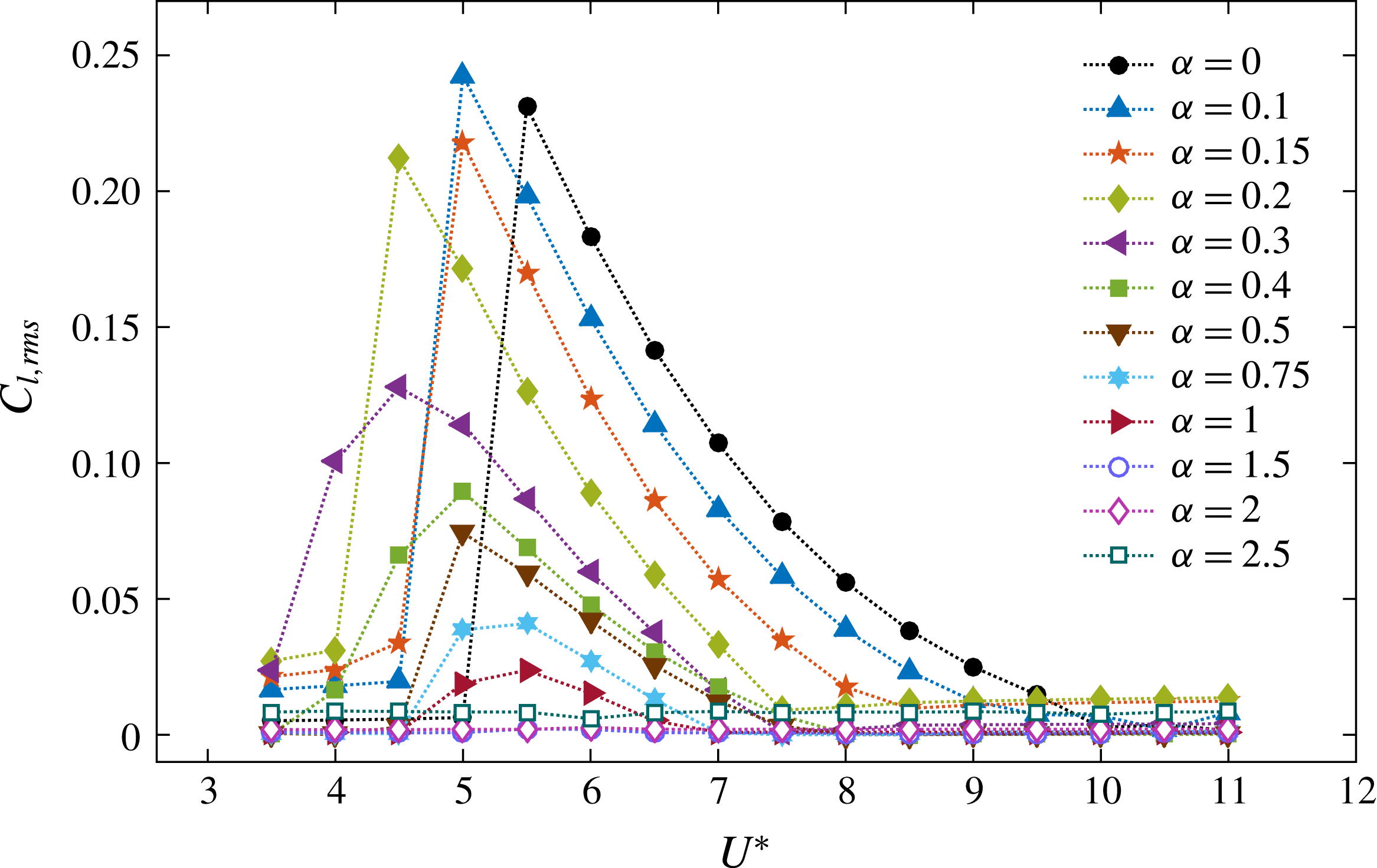
Variation of the r.m.s. value of the time-mean lift force coefficient in the
 $y$
direction over the reduced velocity,
 $U^{\ast }$
, at each rotation rate.

In the synchronisation regimes, the time-mean drag force,
 $\overline{C}_{d}$
, increased from its pre-oscillatory value at each rotation rate. There was a sudden increment at the beginning of the synchronisation regime up to
 $\unicode[STIX]{x1D6FC}=0.2$
. For
 $\unicode[STIX]{x1D6FC}=0$
,
 $\overline{C}_{d}$
decreased throughout the synchronisation range, asymptoting to its pre-oscillatory value at the end of the range. For
 $\unicode[STIX]{x1D6FC}=0.1$
,
 $0.15$
and
 $0.2$
,
 $\overline{C}_{d}$
increased slightly, then decreased during the synchronisation regimes and reached the pre-oscillatory value at the end of the regimes. For
 $0.3\leqslant \unicode[STIX]{x1D6FC}\leqslant 1$
,
 $\overline{C}_{d}$
increased and decreased gradually, similar to the gradual increase and decrease of the vibration amplitude of the sphere at these rotation rates.
Figure 13 shows the variation of the r.m.s. value of the fluctuation component of the lift force coefficient,
 $C_{l}^{\prime }$
, with the reduced velocity, at each rotation rate. Similar to the time-mean components of the forces, the fluctuation components of the forces were also modified in the synchronisation regime at each rotation rate. For
 $\unicode[STIX]{x1D6FC}\leqslant 0.2$
,
 $C_{l}^{\prime }$
increased suddenly from
 $0$
to a value of
 $\simeq 0.22$
at the beginning of the synchronisation regime. Thereafter,
 $C_{l}^{\prime }$
decreased within the synchronisation range and returned to its original value at the end of the range. For
 $0.3\leqslant \unicode[STIX]{x1D6FC}\leqslant 1$
,
 $C_{l}^{\prime }$
increased and then decreased gradually over the synchronisation range. The pattern of variation of
 $C_{l}^{\prime }$
closely matches the pattern of amplitude response (both
 $C_{l}^{\prime }$
and
 $A^{\ast }$
increased suddenly for
 $\unicode[STIX]{x1D6FC}\leqslant 0.2$
and increased gradually for
 $0.3\leqslant \unicode[STIX]{x1D6FC}\leqslant 1$
). Also,
 $C_{l}^{\prime }$
decreased as the rotation rate increased, similar to the trend of
 $A^{\ast }$
with
 $\unicode[STIX]{x1D6FC}$
.
As discussed by Govardhan & Williamson (Reference Govardhan and Williamson2005), the fluid force in the
 $y$
direction,
 $F_{total}$
, can be split into a potential force component,
 $F_{potential}=-m_{A}\ddot{y} (t)$
, which arises due to the potential added-mass force, and a vortex force component,
 $F_{vortex}$
, from the presence and dynamics of vorticity. This recognises the fact that a flow solution can be constructed as a sum of a potential flow field plus a velocity field associated with vorticity in the flow (e.g. see Lighthill Reference Lighthill1986). Here,
 $m_{A}$
is the added mass due to the acceleration of the sphere. Therefore, the vortex force can be computed from
 $$\begin{eqnarray}F_{vortex}=F_{total}-F_{potential}.\end{eqnarray}$$
Normalising all forces by
 $0.5\unicode[STIX]{x1D70C}U^{2}\unicode[STIX]{x03C0}D^{2}/4$
gives,
 $$\begin{eqnarray}C_{vortex}=C_{total}-C_{potential}.\end{eqnarray}$$
The phase between the sphere displacement and
 $C_{total}$
is defined as the total phase,
 $\unicode[STIX]{x1D719}_{total}$
, while the phase between sphere displacement and
 $C_{vortex}$
is defined as the vortex phase,
 $\unicode[STIX]{x1D719}_{vortex}$
.
Govardhan & Williamson (Reference Govardhan and Williamson2005) observed two distinct modes of vibration (modes I and II) for a non-rotating sphere in the reduced-velocity range
 $U^{\ast }\sim 5$
–
 $10$
. In their study, mode I occurred at the beginning of the synchronisation regime and it smoothly transitioned into mode II as the reduced velocity was increased. They observed that
 $\unicode[STIX]{x1D719}_{vortex}$
increased by
 ${\sim}90^{\circ }$
as the sphere vibration transitioned from mode I to mode II. Moreover, they observed little variation in
 $\unicode[STIX]{x1D719}_{total}$
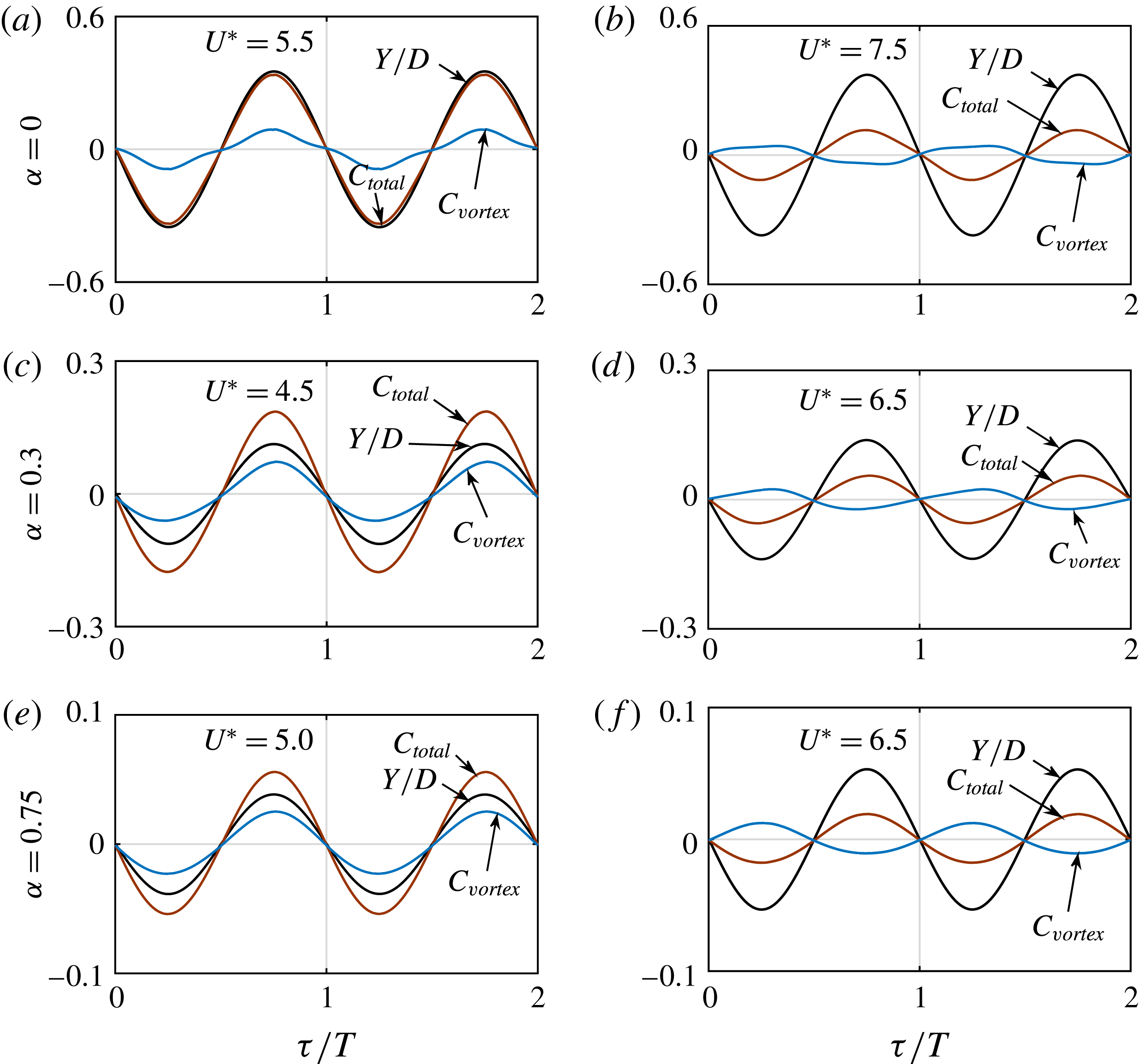
as the mode transitioned from mode I to mode II. Under sphere rotation, a similar behaviour might be expected. Figure 14 shows a comparison of sphere displacement,
 $Y/D$
,
 $C_{total}$
and
 $C_{vortex}$
for two cycles of sphere oscillation for
 $\unicode[STIX]{x1D6FC}=0$
,
 $0.3$
and
 $0.75$
at the beginning of the synchronisation regime (a,c,e) and towards the end of the synchronisation regime (b,d,f). The sphere vibration frequency was locked in to both
 $C_{total}$
and
 $C_{vortex}$
, and was phase aligned with
 $C_{total}$
throughout the synchronisation regime at each
 $\unicode[STIX]{x1D6FC}$
. Moreover, at the beginning of the synchronisation regime, the sphere vibration frequency was phase aligned with
 $C_{vortex}$
. However, it showed a
 $180^{\circ }$
phase difference with
 $C_{vortex}$
towards the end of the regime. Nonetheless, under the conditions of zero damping and near sinusoidal forcing, it is not clear this can be taken as an indication of an analogous transition from mode I to mode II.
Relationship between the time-mean displacement of the sphere,
 $Y/D$
, the total force in the
 $y$
direction,
 $C_{total}$
, and the vortex force in the
 $y$
direction,
 $C_{vortex}$
, at
 $\unicode[STIX]{x1D6FC}=0$
,
 $0.3$
and
 $0.75$
: (a,c,e) at mode I, and (b,d,f) at mode II.

4.3 Wake structures
Vortical structures in the wake are depicted using iso-surfaces of the second invariant of the velocity field (known as the
 $Q$
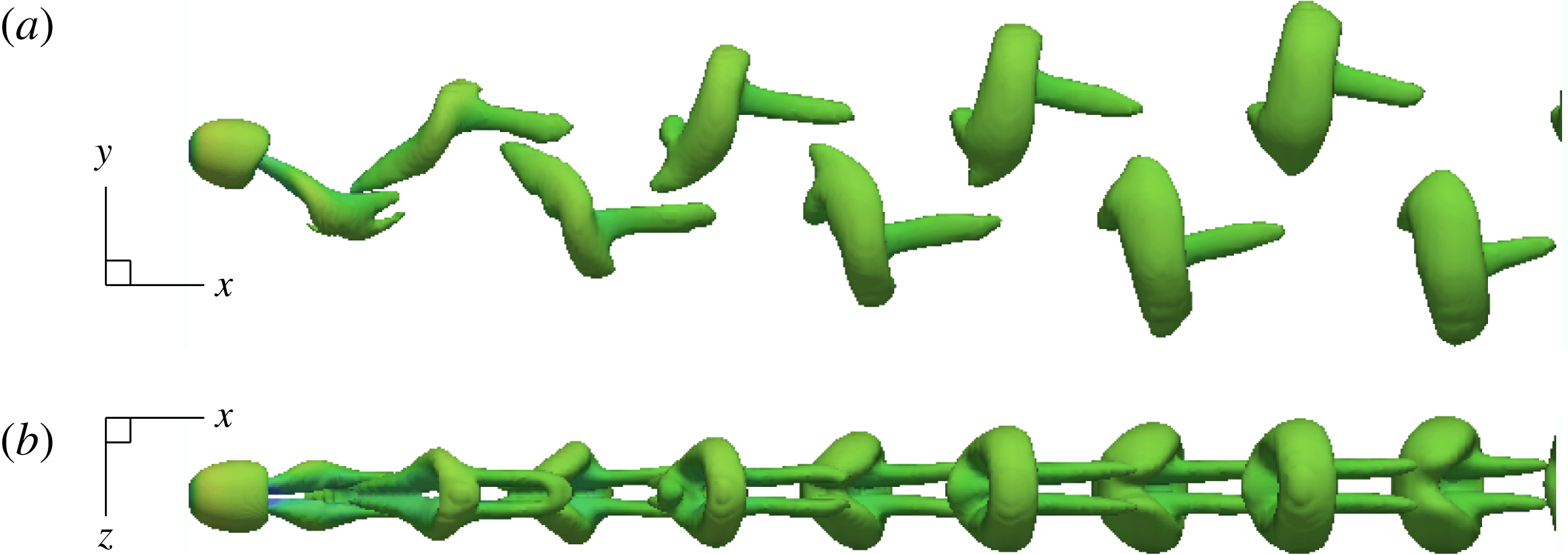
-criterion, see Hunt, Wray & Moin (Reference Hunt, Wray and Moin1988) for more details). Figure 15 displays the wake structure observed in the synchronisation regime of the non-rotating case (at
 $U^{\ast }=6$
). As can be seen, two regular symmetrical streets of hairpin vortices form the wake, consistent with the mode I and II wake structure observed by Govardhan & Williamson (Reference Govardhan and Williamson2005) in their experimental study of vortex-induced vibration of a tethered sphere. This wake structure was also observed by Behara et al. (Reference Behara, Borazjani and Sotiropoulos2011) for VIV of a sphere with 3 DOF at
 $Re=300$
, when the sphere was undergoing planar oscillations. The vortex streets in the advancing and the retreating sides of the sphere were equal in strength, and the sphere oscillation is symmetric through its initial position.
Instantaneous wake structures visualised by the
 $Q$
criterion (
 $Q=0.001$
) in the synchronisation regime of the non-rotating case at
 $U^{\ast }=6$
.

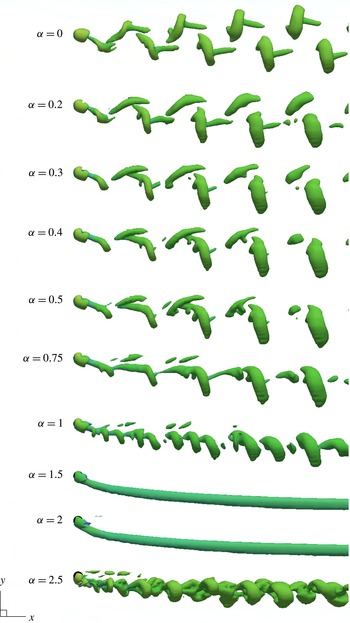
Instantaneous wake structures of vortex-induced vibration of a transversely rotating sphere at reduced velocity
 $U^{\ast }=6$
at each rotation rate. The sphere showed synchronised vibrations up to
 $\unicode[STIX]{x1D6FC}=1$
, and all the synchronisation regimes contained
 $U^{\ast }=6$
. Therefore, the wake structures given for
 $0\leqslant \unicode[STIX]{x1D6FC}\leqslant 1$
are those in the synchronisation regimes at those rotation rates. The Reynolds number of the flow is
 $Re=300$
.

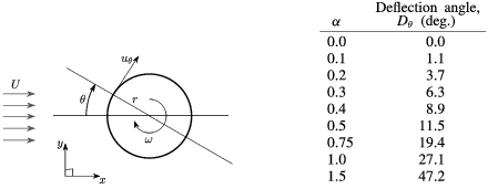
Comparison of the phase-averaged wake deflection angle,
 $D_{\unicode[STIX]{x1D703}}$
, with the rotation rate,
 $\unicode[STIX]{x1D6FC}$
.

As discussed in § 3.1, the wake structure of a flow past a rigidly mounted sphere was modified when a rotation was imposed on the sphere. Similarly, various wake structures were observed for an elastically mounted sphere at different rotation rates and at different reduced velocities. Figure 16 shows the wake structures observed at the reduced velocity,
 $U^{\ast }=6$
, at each rotation rate. As a rotation was imposed on the sphere, the wake was deflected to the advancing side (the negative
 $y$
direction). Moreover, this deflection was more prominent as the rotation rate increased (see figure 16). This is consistent with the lift force applied on the sphere on the retreating side (the positive
 $y$
direction) due to the Magnus effect.
The wake deflection was quantified by observing the change of the shear strain rate along the sphere surface based on the time-mean velocity field. The wake deflection angle,
 $D_{\unicode[STIX]{x1D703}}$
, was defined as the angle at which the shear strain rate in the tangential direction,
 $\unicode[STIX]{x1D716}_{\unicode[STIX]{x1D703}}$
, on the sphere surface at the
 $xy$
plane was zero (
 $D_{\unicode[STIX]{x1D703}}=\unicode[STIX]{x1D703}|_{\unicode[STIX]{x1D716}_{\unicode[STIX]{x1D703}}=0}$
). This parameter (
 $\unicode[STIX]{x1D716}_{\unicode[STIX]{x1D703}}$
) can be calculated by taking the derivative of tangential velocity,
 $u_{\unicode[STIX]{x1D703}}$
, in the radial direction,
 $\text{d}(u_{\unicode[STIX]{x1D703}})/\text{d}r$
. Therefore, the wake deflection angle,
 $D_{\unicode[STIX]{x1D703}}$
, was the angle,
 $\unicode[STIX]{x1D703}$
, at which
 $\text{d}(u_{\unicode[STIX]{x1D703}})/\text{d}r=0$
. The variation of the phase-averaged wake deflection angle,
 $D_{\unicode[STIX]{x1D703}}$
, with the rotation rate is tabulated in table 3. As can be seen,
 $D_{\unicode[STIX]{x1D703}}$
increased with the rotation rate. This quantifies the observations from visualisations that the deflection was more prominent at higher rotation rates.
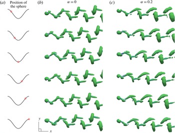
Evolution of wake structures for one cycle of sphere oscillation in the synchronisation regimes (at
 $U^{\ast }=6$
) for the rotation rates
 $\unicode[STIX]{x1D6FC}=0$
and
 $0.2$
. The first column displays the position of the sphere by a red ‘bullseye’ on a cosine wave for one period, while the second and third columns show the instantaneous wake structures observed at each of these positions of the sphere for
 $\unicode[STIX]{x1D6FC}=0$
and
 $0.2$
, respectively.

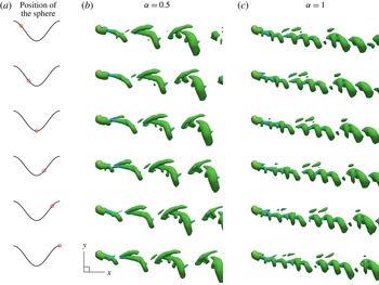
The equal strength vortex streets at zero rotation, became unequal as the sphere rotation rate was increased (see figure 16). The vortex street on the advancing side became stronger than the one in the retreating side with increasing rotation rate. The vortex street on the retreating side was greatly weakened for
 $\unicode[STIX]{x1D6FC}=0.75$
, and had largely disappeared for
 $\unicode[STIX]{x1D6FC}\in [1,1.3]$
. This difference in the strength of the vortex streets, which affects the oscillatory forces on the sphere, is consistent with the decrease in the oscillation amplitude as the sphere rotation rate increased.
When the sphere was subjected to a rotation, there was a significant variation in the structure of the wake in the synchronisation regime. The vortex loops on the advancing side were closely spaced hairpin loops. However, the vortex loops on the retreating side deviated from the hairpin type as the rotation rate increased. Moreover, for
 $0.3\leqslant \unicode[STIX]{x1D6FC}\leqslant 1.3$
, the vortex loops on the retreating side near the sphere were attached to the vortex loops on the advancing side that were shed in the previous cycle. However, they separated later as they moved further downstream.
Evolution of the wake structures for one cycle of the sphere oscillation in the synchronisation regimes (at
 $U^{\ast }=6$
) for the rotation rates
 $\unicode[STIX]{x1D6FC}=0.5$
and
 $1$
. The first column displays the position of the sphere by a red ‘bullseye’ on a cosine wave for one period, while the second and third columns show the instantaneous wake structures observed at each of these positions of the sphere for
 $\unicode[STIX]{x1D6FC}=0.5$
and
 $1$
respectively.

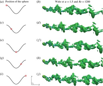
Figures 17 and 18 show the evolution of wakes in the synchronisation regimes (at
 $U^{\ast }=6$
) over a cycle of sphere oscillation for the rotation rates
 $\unicode[STIX]{x1D6FC}=0$
,
 $0.2$
,
 $0.5$
and
 $1$
. A vortex loop is shed from the retreating side of the sphere as the sphere moved from its apex to its nadir at both
 $\unicode[STIX]{x1D6FC}=0$
and
 $0.2$
(see figure 17). Another loop is shed from the advancing side half a cycle later. For
 $\unicode[STIX]{x1D6FC}=0$
, the vortex loops were disconnected from each other and formed with a tail. The tail was co-directional with the streamlines upstream. As the loops moved away from the sphere, their shapes changed from a hairpin to a ring shape. In addition to that, the vortex loops on the advancing and the retreating sides are mirror images (with a
 $180^{\circ }$
phase delay) consistent with the symmetric sphere oscillation. However, for
 $\unicode[STIX]{x1D6FC}=0.2$
, in line with the non-zero time-mean lift force applied on the sphere on the retreating side (
 $y$
direction), a vortex loop on the retreating side is shed weakly compared to the one on the advancing side. Moreover, the wake was deflected to the advancing side, and the vortex street on the advancing side was stronger. For
 $\unicode[STIX]{x1D6FC}=0.5$
, a vortex loop on the retreating side was shed far more weakly and appeared only when the sphere was near its nadir (see figure 18). A vortex loop on the advancing side was also modified compared to that at
 $\unicode[STIX]{x1D6FC}=0$
and its tail had almost disappeared.
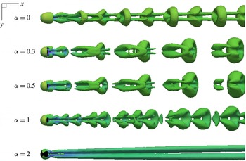
Instantaneous wake structures in the
 $xz$
plane for a transversely rotating sphere at
 $U^{\ast }=6$
for the rotation rates
 $\unicode[STIX]{x1D6FC}=0$
,
 $0.3$
,
 $0.5$
,
 $1$
and
 $2$
.

On increasing
 $\unicode[STIX]{x1D6FC}$
toward one, vortex loops shed from the retreating side were weak, with the standard sphere wake with long interlacing vortex loops replaced by a different wake structure, with closely spaced loops originating from the boundary layer/shear layer separating from the sphere. This wake structure resembled the wake structure observed by Giacobello et al. (Reference Giacobello, Ooi and Balachandar2009) and Kim (Reference Kim2009) for the flow past a transversely rotating sphere at
 $Re=300$
and
 $\unicode[STIX]{x1D6FC}=1$
. Kim (Reference Kim2009) argued that this unsteadiness was due to the instability of the shear layer caused by rapid rotation. For flow past a transversely rotating rigid sphere at these parameters, we also observed a similar wake structure but only in the initial stage of the simulation as discussed in § 3.1; however, the shedding faded away for long simulation times, and the flow became steady asymptotically. Despite this, when the sphere was allowed to translate in the
 $y$
direction, the sphere maintained a small amplitude vibration over a narrow reduced velocity range, even after long integration times.
The wake at
 $\unicode[STIX]{x1D6FC}=1$
and
 $U^{\ast }=6$
shows vortex loops or hairpins, but the wake frequency is approximately a factor of three higher. Thus at
 $U^{\ast }=6$
, approximately three vortex loops are shed per system oscillation period. However, the shed loops are not identical in the size, nor are they exactly locked to have three shedding periods per vibration period. In this case, the near wake oscillates with the body oscillation at a frequency close to that of a non-vibrating sphere at a lower rotation rate. One possible interpretation is that the natural vortex-shedding instability of the wake, which is suppressed by the development of the shear-layer instability, is still receptive, so that if the sphere is allowed to oscillate at that frequency, that shedding mode can reappear and sustain the oscillation. This study at
 $\unicode[STIX]{x1D6FC}=1$
was expanded to lower reduced velocities. At
 $U^{\ast }=2$
, where the system frequency matches the shear-layer mode shedding frequency, the body vibration is minimal even through the wake is strongly periodic. In this case, it appears that the timing of the formation and shedding of shear-layer vortices does not lead to positive energy transfer from the fluid to the body, so that large amplitude oscillations do not occur.
A steady wake was observed at the rotation rates
 $\unicode[STIX]{x1D6FC}=1.5$
and
 $2$
for all the reduced velocities considered, as shown in figure 16 at
 $U^{\ast }=6$
. This confirms that the sphere vibrations were completely suppressed for
 $\unicode[STIX]{x1D6FC}>1.3$
. For
 $\unicode[STIX]{x1D6FC}=2.5$
, an unsteady and asymmetric wake was observed for all the reduced velocities considered, with a structure shown in figure 16 at
 $U^{\ast }=6$
. Even though the flow was unsteady with vortex shedding at this rotation rate, no significant sphere vibration was observed.
Figure 19 shows the wake structures in the
 $xz$
plane at
 $U^{\ast }=6$
for the rotation rates
 $\unicode[STIX]{x1D6FC}=0.1$
,
 $0.3$
,
 $1$
,
 $2$
and
 $2.5$
. As can be seen, all the structures observed for
 $\unicode[STIX]{x1D6FC}\leqslant 2$
were mirror symmetric about the
 $xy$
plane, except the wake at
 $\unicode[STIX]{x1D6FC}=2.5$
.
As discussed in § 3.1, the flow past a transversely rotating rigid sphere showed unsteady vortex shedding for
 $\unicode[STIX]{x1D6FC}\in [0,0.3]$
, and a double-threaded wake for
 $\unicode[STIX]{x1D6FC}\in [0.4,2]$
. When the sphere was allowed to oscillate in the
 $y$
direction, the sphere showed synchronised vibrations for
 $\unicode[STIX]{x1D6FC}\leqslant 1.3$
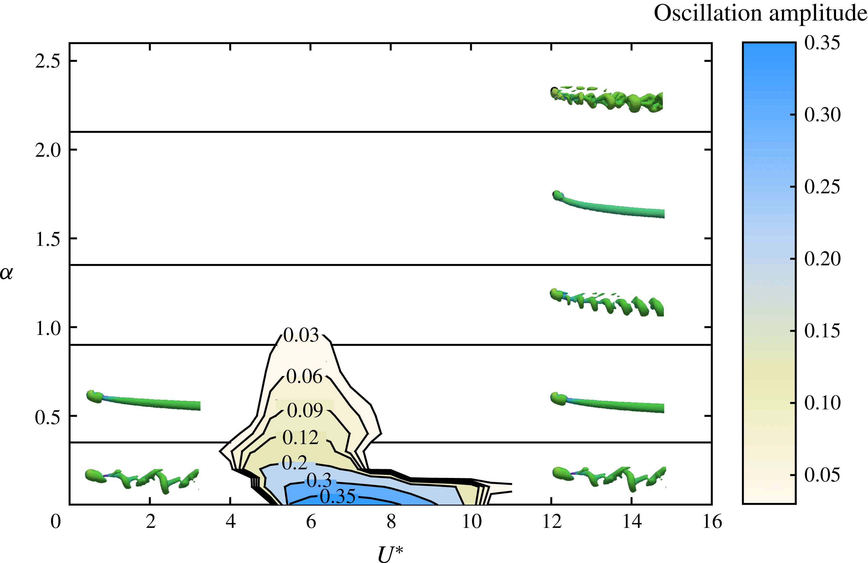
. At these rotation rates, outside the synchronisation regimes, a few different wake structures were observed, depending on the rotation rate. These different wake states are depicted in figure 20, together with a contour map summarising the oscillation amplitude as a function of
 $U^{\ast }$
and
 $\unicode[STIX]{x1D6FC}$
. The contour map shows the reduction of the oscillation amplitude and narrowing of the synchronisation regime as the rotation rate is increased. Outside the synchronisation regime, for
 $\unicode[STIX]{x1D6FC}\in [0,0.3]$
, unsteady vortex shedding was observed, while for
 $\unicode[STIX]{x1D6FC}\in [0.4,0.75]$
, a steady and a double-threaded wake was found to occur; both states are consistent with rigid sphere wakes at the same rotation rates. However, for
 $\unicode[STIX]{x1D6FC}=1$
, outside the synchronisation regime, an unsteady wake was observed (see figure 20). This wake resembled the wake observed in the initial evolution stage for a rigidly mounted sphere at the same rotation rate, for which the unsteady wake observed in the initial stage transformed into a steady wake in the asymptotic stage. However, given the possibility to oscillate, albeit at very small amplitude, the unsteadiness of the wake persisted.
Contour plot of the sphere oscillation amplitude,
 $A^{\ast }$
, as a function of the reduced velocity,
 $U^{\ast }$
, and rotation rate,
 $\unicode[STIX]{x1D6FC}$
. The non-synchronisation regime is divided into five regimes according to wake structures.

5 The effect of Reynolds number on VIV of a rotating sphere
The effect of Reynolds number on vortex-induced vibration of a rotating sphere was investigated at three rotation rates,
 $\unicode[STIX]{x1D6FC}=0.15$
,
 $0.75$
and
 $1.5$
, by fixing the reduced velocity at
 $U^{\ast }=6$
. These three rotation rates were chosen because at
 $\unicode[STIX]{x1D6FC}=0.15$
and
 $0.75$
, the sphere showed synchronised vibration, whilst at
 $\unicode[STIX]{x1D6FC}=1.5$
, the flow was steady and no sphere vibration was found, but noting that this was not the case in higher Reynolds number experiments (Sareen et al.
Reference Sareen, Zhao, Lo Jacono, Sheridan, Hourigan and Thompson2018). In addition to that, for flow past a rotating sphere, at
 $Re=300$
, the wake was unsteady with vortex shedding at
 $\unicode[STIX]{x1D6FC}=0.15$
while the flow was steady at
 $\unicode[STIX]{x1D6FC}=0.75$
. In this investigation, the Reynolds number of the flow was varied from
 $300$
to
 $1200$
while keeping the mass ratio of the sphere fixed at
 $m^{\ast }=2.865$
.
5.1 Mean displacement, amplitude and forces
Figure 21 shows the variation of the sphere response amplitude with Reynolds number for
 $\unicode[STIX]{x1D6FC}=0.15$
,
 $0.75$
and
 $1.5$
at
 $U^{\ast }=6$
. At
 $\unicode[STIX]{x1D6FC}=0.15$
and
 $Re=300$
, the sphere vibrated synchronously with the vortex-shedding frequency with an amplitude of
 ${\approx}0.3D$
. As can be seen from figure 21, at
 $\unicode[STIX]{x1D6FC}=0.15$
, the sphere response amplitude increased with increasing Reynolds number and reached a value of
 ${\approx}0.5D$
at
 $Re=1200$
. At each of these Reynolds numbers, the sphere vibration was highly sinusoidal. This suggests that even for the non-rotating case, the sphere response amplitude will increase with increasing Reynolds number, which is consistent with the large amplitude response observed in non-rotating sphere VIV experiments (e.g. Govardhan & Williamson Reference Govardhan and Williamson1997, Reference Govardhan and Williamson2005, Jauvtis et al.
Reference Jauvtis, Govardhan and Williamson2001).
Effect of Reynolds number on the sphere response amplitude at the rotation rates,
 $\unicode[STIX]{x1D6FC}=0.15$
,
 $0.75$
and
 $1.5$
at
 $U^{\ast }=6$
.

Similar to the case of
 $\unicode[STIX]{x1D6FC}=0.15$
, at
 $\unicode[STIX]{x1D6FC}=0.75$
, the sphere vibration amplitude showed an increasing trend with increasing Reynolds number. However, a slight decrement in
 $A^{\ast }$
was observed from
 $Re=550$
to
 $600$
. The sphere vibration was purely sinusoidal up to
 $Re=500$
. For
 $Re\geqslant 550$
, even though the sphere response was periodic, it was less sinusoidal. The periodicity of a signal was defined as
 $\unicode[STIX]{x1D706}_{A}=\sqrt{2}Y_{rms}/Y_{max}$
(Jauvtis et al.
Reference Jauvtis, Govardhan and Williamson2001), where
 $Y_{max}$
is the highest sphere amplitude recorded. According to this definition,
 $\unicode[STIX]{x1D706}_{A}$
can take values from
 $0$
to
 $1$
, with
 $\unicode[STIX]{x1D706}_{A}=1$
for a purely sinusoidal signal. Figure 22 shows the variation of periodicity of the sphere response with Reynolds number for
 $\unicode[STIX]{x1D6FC}=0.15$
,
 $0.75$
and
 $1.5$
. As can be seen, at
 $\unicode[STIX]{x1D6FC}=0.75$
, the periodicity of the signal starts to drop for
 $Re$
greater than 550. Moreover,
 $\unicode[STIX]{x1D706}_{A}$
drops to
 ${\approx}0.85$
and remains there for
 $Re\geqslant 600$
.
Variation of the periodicity of sphere response,
 $\unicode[STIX]{x1D706}_{A}$
, with Reynolds number at
 $\unicode[STIX]{x1D6FC}=0.15$
,
 $0.75$
and
 $1.5$
for
 $U^{\ast }=6$
.

Effect of Reynolds number on (a) time-mean position of the sphere, (b) time-mean lift coefficient, (c) frequency ratio and (d) time-mean drag coefficient, at the rotation rates
 $\unicode[STIX]{x1D6FC}=0.15$
,
 $0.75$
and
 $1.5$
.

Effect of Reynolds number on the wake structures (depicted with
 $Q=0.01$
) at the rotation rates
 $\unicode[STIX]{x1D6FC}=0.15$
,
 $0.75$
and
 $1.5$
. The reduced velocity of the flow is
 $U^{\ast }=6$
for each case.

At
 $\unicode[STIX]{x1D6FC}=1.5$
and
 $Re=300$
, the flow was steady with no sphere vibration. This behaviour continued at
 $Re=350$
, as well. However, as the Reynolds number was increased from
 $400$
, the sphere started to show synchronised vibration again. The sphere response amplitude increased with the increasing Reynolds number and reached a value of
 ${\approx}0.25D$
at
 $Re=1200$
. The sphere response was periodic, but was less sinusoidal. The periodicity of the sphere response showed a slight increasing trend with Reynolds number, with values around
 $0.8$
(see figure 22).
At each of the rotation rates and Reynolds numbers considered, the sphere vibration frequency was locked in with the frequency of the lift force (reflecting the vortex shedding). Moreover, the sphere vibration frequency was close to the system’s natural frequency (
 $f^{\ast }\approx 1$
, see figure 23
c). Therefore, these vibration states are vortex-induced vibration. From these observations, we can expect that the VIV will occur for even higher rotation rates for higher Reynolds number flows.
Figure 23 shows the variation of the time-mean sphere displacement, the time-mean drag and lift coefficients, and the frequency ratio with Reynolds number for
 $\unicode[STIX]{x1D6FC}=0.15$
,
 $0.75$
and
 $1.5$
. As can be seen, at
 $\unicode[STIX]{x1D6FC}=0.15$
, the time-mean position of the sphere,
 $\overline{Y}/D$
, remained almost fixed for all Reynolds numbers considered. However, at
 $\unicode[STIX]{x1D6FC}=0.75$
and
 $1.5$
,
 $\overline{Y}/D$
decreased with increasing Reynolds number. The time-mean lift coefficient showed an identical trend with the time-mean sphere displacement for all three rotation rates (see figure 23
b). At
 $\unicode[STIX]{x1D6FC}=0.15$
, the time-mean drag coefficient decreased up to
 $Re=600$
, and for higher Reynolds numbers it was almost flat (see figure 23
d). For both
 $\unicode[STIX]{x1D6FC}=0.75$
and
 $1.5$
,
 $\overline{C}_{d}$
decreased with increasing Reynolds number.
5.2 Effect on wake structures
The vortical structure of the wake was observed using the
 $Q$
-criterion with a value of
 $Q=0.01$
. Figure 24 shows the wake structures observed at
 $\unicode[STIX]{x1D6FC}=0.15$
for
 $Re=700$
and
 $1200$
; at
 $\unicode[STIX]{x1D6FC}=0.75$
for
 $Re=500$
,
 $900$
and
 $1200$
; and at
 $\unicode[STIX]{x1D6FC}=1.5$
for
 $Re=900$
and
 $1200$
. At
 $\unicode[STIX]{x1D6FC}=0.15$
, two streets of hairpin-type vortex loops were observed at each Reynolds number. However, as the Reynolds number increased, the shape of the vortex loops were modified slightly (e.g. see the difference between the wakes at
 $Re=700$
and
 $1200$
in figure 24 at
 $\unicode[STIX]{x1D6FC}=0.15$
). The vortex-shedding frequencies were locked in with the sphere vibrations.
The sensitivity of the spatial resolution of the flow parameters of vortex-induced vibration of a rotating sphere at
 $(\unicode[STIX]{x1D6FC},U^{\ast })=(1.5,6)$
and
 $Re=1200$
and
 $m^{\ast }=2.865$
(
 $m_{r}=1.5$
). The oscillation amplitude of the sphere,
 $A^{\ast }$
, the time-mean drag coefficient,
 $\overline{C}_{d}$
, the r.m.s. values of fluctuation component of the drag and lift coefficients,
 $C_{d,rms}$
and
 $C_{l,rms}$
, and the ratio of vortex-shedding frequency to the natural frequency,
 $f/f_{n}$
, are listed.

As a general comment on these simulations, we would certainly not claim that for the higher Reynolds number cases the chaotic wake structures are fully resolved downstream from the near wake. The main aim of this set of simulations was to properly resolve the near wake through increased spatial resolution, which, together with the larger-scale wake structures, should mainly control the VIV response of the sphere. Further spatial resolution studies were undertaken to confirm that the VIV response was well converged at the highest Reynolds number (
 $Re=1200$
) and highest rotation rate (
 $\unicode[STIX]{x1D6FC}=1.5$
) considered (see the table 4). As can be seen, there is less than
 $2\,\%$
variation in the amplitude, drag and frequency ratio for the different grids. Thus, grid
 $2$
could be used; however, it was decided to use grid
 $3$
for the higher Reynolds number simulations presented in this section since this grid is more compressed toward the sphere surface.
As discussed above, at
 $\unicode[STIX]{x1D6FC}=0.75$
, the sphere vibration was purely sinusoidal for
 $Re\in [300,500]$
. In this Reynolds number range, two-sided hairpin-type vortex loops were observed, as shown at
 $Re=500$
. Compared to the wake at
 $Re=300$
shown in figure 16, the wake deflection is smaller and the vortex loops on the retreating side are comparatively stronger at
 $Re=500$
. This can be attributed to the reduction of the mean lift force at higher Reynolds numbers. In the Reynolds number range,
 $Re\in [550,1200]$
, the sphere vibration was less sinusoidal (
 $\unicode[STIX]{x1D706}_{A}\approx 0.8$
). Indeed, in this range, the wake showed a more turbulent behaviour with shedding of multiple vortex structures per sphere oscillation cycle. However, the dominant vortex-shedding frequency was still synchronised with the sphere vibration frequency (see figure 24 wake for
 $Re=900$
and
 $1200$
at
 $\unicode[STIX]{x1D6FC}=0.75$
).
Evolution of the wake at
 $\unicode[STIX]{x1D6FC}=1.5$
,
 $Re=1200$
and
 $U^{\ast }=6$
for a cycle of sphere vibration. The left column shows the sphere position in the cycle with a red ‘bullseye’ on a cosine wave and the right column shows the wake structures observed at corresponding sphere positions.

At
 $\unicode[STIX]{x1D6FC}=1.5$
, the sphere showed synchronised vibrations for
 $Re\in [400,1200]$
. In this Reynolds number range, the sphere vibrations were less sinusoidal. Therefore, similar to
 $\unicode[STIX]{x1D6FC}=0.75$
at higher Reynolds numbers, multiple vortical structures were shed over a sphere vibration cycle, showing chaotic behaviour. Figure 25 shows the evolution of wake structures over a cycle of sphere vibration in five steps for
 $\unicode[STIX]{x1D6FC}=1.5$
and
 $Re=1200$
. Even though multiple vortical structures were shed per sphere oscillation cycle, vortex loops were two sided. In particular, vortex loops were shed from the positive
 $y$
direction as the sphere moved from its apex to its nadir, and vortex loops were shed from the negative
 $y$
direction as the sphere moved from its nadir to its apex. Therefore, the dominant vortex shedding frequency was locked in with the sphere vibration frequency.
6 Conclusions
The effects of forced rotation on transverse vortex-induced vibration of a sphere was investigated numerically at Reynolds number
 $300$
with a sphere of mass ratio
 $2.865$
(corresponding to a reduced mass of 1.5). The correlation between the Magnus effect caused by the sphere rotation and the vortex-induced vibration has been analysed over the reduced-velocity range
 $U^{\ast }\in [3.5,11]$
and rotation rates
 $\unicode[STIX]{x1D6FC}\in [0,2.5]$
. The principal findings of this work can be summarised as follows.
Reduction of the sphere response amplitude with forced rotation. The sphere was found to vibrate, synchronising with the vortex-shedding frequency even subject to an imposed forced rotation. However, the sphere shifted to a new time-mean position for all rotation cases due to the Magnus force generated by the rotation. The sphere showed highly periodic VIV, not only for
 $\unicode[STIX]{x1D6FC}<0.4$
, but also for
 $0.4\leqslant \unicode[STIX]{x1D6FC}\leqslant 1.3$
, i.e. over a range of rotation rates where no vortex shedding was found for a rigidly mounted rotating sphere (at this Reynolds number). Interestingly, the sphere response amplitude, which was
 ${\approx}0.4D$
for the zero rotation case, decreased as the rotation rate increased, and VIV was completely suppressed beyond
 $\unicode[STIX]{x1D6FC}=1.3$
. Simultaneously, the synchronisation range narrowed and moved mostly towards lower values of
 $U^{\ast }$
with increasing rotation rate.
Force coefficients highly modulated in the synchronisation regime. The time-mean lift and drag coefficients were highly modulated as the sphere experienced synchronised vibration. In particular, the time-mean drag force increased while the time-mean lift force decreased from its pre-oscillatory value in the synchronisation regime at each rotation rate. The analysis of phases between sphere displacement and vortex force revealed that, regardless of the rotation rate, the sphere showed similarities to mode I initially and then mode II vibrations identified through total and vortex phase variations.
Symmetry breaking of the wake under forced rotation. In the synchronisation regime of the zero rotation case, two trails of two-sided hairpin loops formed in the wake. Moreover, the vortex trails on the advancing and retreating sides were equal in strength as the sphere oscillation was symmetric about its initial position. These wake states strongly resemble those of a tethered sphere observed experimentally by Govardhan & Williamson (Reference Govardhan and Williamson2005) at much higher
 $Re$
, for both modes I and II. As a rotation was imposed on the sphere, the wake deflected to the advancing side (
 $-y$
direction); this was more prominent as the rotation rate increased. With the symmetry breaking of the wake introduced by the Magnus effect, the vortex loops in the vorticity trail from the advancing side became stronger than the vortex loops in the trail from the retreating side. This unevenness of the wake, which affects the oscillatory forces on the sphere, is consistent with the reduction in the amplitude response and narrowing of the synchronisation range at higher rotation rates.
The response amplitude increased significantly as Reynolds number was increased. The effect of Reynolds number on VIV of a rotating sphere was investigated at
 $U^{\ast }=6$
, by increasing Reynolds number incrementally up to
 $Re=1200$
. As the Reynolds number was increased, the sphere started to show synchronised vibration at higher rotation rates even when there was no VIV at
 $Re=300$
. In addition, the sphere response amplitude increased generally with the increasing Reynolds number. Therefore, at higher Reynolds numbers, VIV persists for even higher rotation rates and displays a large amplitude response, consistent with experimental studies by Sareen et al. (Reference Sareen, Zhao, Lo Jacono, Sheridan, Hourigan and Thompson2018).
Based on the above observations, we can draw the following conclusions: vortex-induced vibration persists for a sphere at small rotation rates, but the mitigation/suppression of vortex shedding caused by the Magnus effect as the rotation rate is increased does in fact lead to increased suppression of VIV at higher rotation rates. Moreover, spanning the laminar regime and beyond, the effect of Reynolds number on the VIV response of a rotating sphere is significant.
In terms of future work, it seems worth expanding this study further into the fully turbulent regime where most experiments are conducted. It would also be interesting to examine the response of a heavier sphere at higher reduced velocities, where modes III and IV are observed to occur.
Acknowledgements
The support from Australian Research Council Discovery grants DP130100822, DP150102879 and DP170100275, computing time available through Merit Project grants n67 and d71 through the National Computational Infrastructure (NCI), and the Pawsey Supercomputing Centre are gratefully acknowledged.