1. Introduction
External flows around obstacles immersed in a fluid stream are very common in science and engineering. These flows have the distinctive characteristic of involving strong viscous effects near the body surface and in the wake behind it, while being nearly inviscid far from the obstacle. Moreover, they inherently represent a multiscale problem, which involves many complex fluid dynamics phenomena. The presence of flow separation and reattachment, curved shear layers and the relatively low Reynolds number transition to turbulence (Lyn et al. Reference Lyn, Einav, Rodi and Park1995) makes numerical simulations computationally expensive even for simple flow geometries. For instance, the prediction of the unsteady aerodynamic forces arising from flow–structure interaction remains a challenging issue for a number of fundamental technological applications. To capture the essential structure of the turbulent shedding flow around the body, the computational grid must be properly refined both close to the body surface, to resolve the kinematic boundary layer, and behind the obstacle, to simulate the wake flow accurately. In addition, the simulation of the flow around two-dimensional bodies requires the use of a sufficiently large spanwise domain in order not to alter the physical spatial coherency. Hence, the direct numerical simulation (DNS) of turbulent flow past solid obstacles is practically not affordable, even at moderately high Reynolds numbers. On the other hand, flows involving massive separation represent a very difficult class of problems for Reynolds-averaged Navier–Stokes (RANS) methods, mainly due to their inability to capture unsteady flow characteristics related to organized large-scale time-varying flow motions.
With the growth of computer power, the use of the higher fidelity large-eddy simulation (LES) approach has become a practical alternative for simulating external flows. The LES method allows the three-dimensional time-dependent solution of the Navier–Stokes equations to be achieved, with computational cost between DNS and RANS. In the LES framework, the wall layer, where viscous shear stresses are dominant, can be either directly computed, which is referred to as wall-resolving LES, or approximated by means of a specific model, which is referred to as wall-modelling LES. The former approach is more accurate but computationally much more expensive due to the almost DNS-like near-wall resolution required to enforce the no-slip boundary condition. Since the size of the flow structures that are responsible for the turbulent production decreases with increasing Reynolds number, the wall-resolving LES method is limited to moderately high Reynolds number flows. To bypass this issue, a number of hybrid RANS/LES methods have been proposed, where the two different approaches are blended together. Namely, different zones of the flow field, which are determined through the use of either a zonal scheme or a smooth blending parameter, are computed by means of the two different methodologies (Fröhlich & von Terzi Reference Fröhlich and von Terzi2008; Spalart Reference Spalart2009). In addition, taking advantage of the turbulence intermittency, adaptive mesh refinement (AMR) techniques can be used for reducing the number of unnecessary grid points, while increasing the numerical resolution only in the regions of interest, e.g. Vanella, Rabenold & Balaras (Reference Vanella, Rabenold and Balaras2010).
The wavelet transform has become a well-established tool for the analysis of turbulence, where the turbulent velocity field is decomposed into modes that are localized in both wavenumber and physical space, e.g. Meneveau (Reference Meneveau1991), Farge (Reference Farge1992). Moreover, wavelet-based methods have been successfully developed to reduce the computational complexity of numerical simulations, while capturing the essential physics of turbulent flows (Schneider & Vasilyev Reference Schneider and Vasilyev2010). In this study, the natural ability of wavelet multi-resolution analysis to identify and track energy-containing motions is exploited to construct a high-fidelity physics-based adaptive LES method for bluff-body flows. The energy-carrying structures are resolved down to the wall, while the numerical resolution is automatically adapted to the local flow conditions. By decomposing the velocity field in terms of wavelet basis functions and retaining only significant wavelets, the degrees of freedom of the numerical solution and, thus, the associated computational cost can be drastically reduced with respect to non-adaptive methods. The actual importance of the unresolved velocity field is controlled by the wavelet thresholding level that is prescribed. For very low thresholds, the residual background flow can be completely neglected, resulting in the wavelet-based direct numerical simulation (WDNS) method. For slightly higher levels, the effect of the residual motions can be approximated by Gaussian white noise, which is typically not modelled, leading to the coherent vortex simulation (CVS) approach (Farge, Schneider & Kevlahan Reference Farge, Schneider and Kevlahan1999). Eventually, the use of relatively high thresholding levels necessitates the introduction of a subgrid-scale model that mimics the effect of the unknown residual motions, which is referred to as wavelet-based adaptive large-eddy simulation (LES) methodology (Goldstein & Vasilyev Reference Goldstein and Vasilyev2004).
In practice, the abovementioned wavelet-based approaches employ the same high-order adaptive wavelet-collocation (AWC) method to resolve energy-containing/dynamically important eddies on a near optimal computational grid that automatically adapts to the solution, e.g. Vasilyev & Kevlahan (Reference Vasilyev and Kevlahan2005). Due to the built-in wavelet-based grid adaptation, the spatially non-uniform meshing is not prescribed a priori, but dynamically determined according to the evolution of the flow field. In fact, the mesh is automatically refined where high gradients in the solution exist, thus ensuring the adequate resolution of the most important flow structures. Due to this commonality, WDNS, CVS and wavelet-based adaptive LES are all referred to as eddy-capturing approaches (De Stefano & Vasilyev Reference De Stefano and Vasilyev2012).
When dealing with flow past solid obstacles, the AWC method has been successfully used in conjunction with the Brinkman volume-penalization method, which allows one to mimic the presence of the body without resorting to complex body-fitted computational meshes. The method practically consists in the slight modification of the governing equations by adding an appropriate forcing term (Angot, Bruneau & Fabrie Reference Angot, Bruneau and Fabrie1999). The hybrid wavelet-collocation/volume-penalization method for flow–structure interaction has recently been extended to wall-bounded three-dimensional incompressible flows by De Stefano & Vasilyev (Reference De Stefano and Vasilyev2014).
Until recently, the various wavelet-based turbulence modelling approaches have employed an a priori defined constant thresholding level. For homogeneous turbulent flows, an alternative fully adaptive method based on spatially uniform time-dependent thresholding was recently proposed by De Stefano & Vasilyev (Reference De Stefano and Vasilyev2012). The robustness of the wavelet-based approach to homogeneous turbulence simulation has been further improved by introducing the physics-based spatio-temporally variable thresholding strategy. The method adjusts the wavelet threshold to achieve spatially uniform turbulence resolution and fully exploits the intermittency of turbulence by solving a Lagrangian evolution equation for the threshold field (Nejadmalayeri et al. Reference Nejadmalayeri, Vezolainen, De Stefano and Vasilyev2014).
The main objective of the present study is to extend the wavelet-based eddy-capturing approach with Lagrangian variable thresholding to the simulation of wall-bounded turbulent flows, where the flow geometry is enforced through Brinkman volume penalization. Use of the AWC method with a varying wavelet threshold allows the fidelity of the numerical solution to be directly controlled so that the level of desired turbulence resolution can be prescribed by the user. New forcing mechanisms for bluff-body flows are proposed and demonstrated for incompressible turbulent flow around an isolated stationary prism with square cross-section at moderately high Reynolds number.
The remainder of this paper is organized as follows. In § 2, the wavelet-based combined volume-penalization/eddy-capturing approach for the adaptive LES of incompressible turbulent immersed-body flows is presented. The energy-based one-equation model for the closure of the LES problem is reviewed in § 3. The new Lagrangian variable thresholding method for bluff-body flows is introduced in § 4, while the results of the numerical experiments for square cylinder flow are presented and discussed in § 5. Finally, some concluding remarks are made in § 6.
2. Methodology
The proposed computational methodology combines the Brinkman volume-penalization technique with the AWC method, with the former being responsible for imposing the flow geometry and the latter guaranteeing the efficient resolution of the flow on a dynamically adaptive computational grid. In the following, the two building blocks are briefly reviewed, along with the resulting wavelet-based adaptive LES approach for external flows.
2.1. Volume penalization
For the sake of simplicity, the volume-penalization method is presented for the case of a single body, but the procedure can be easily generalized to flows past multiple bodies (Angot et al.
Reference Angot, Bruneau and Fabrie1999). Instead of solving the incompressible Navier–Stokes equations in the fluid domain, say
 ${\it\Omega}_{f}$
, with the associated no-slip boundary condition on the body surface, the following continuity and momentum equations for the penalized perturbation velocity
 $u_{i}$
are considered:
 $$\begin{eqnarray}\displaystyle & \displaystyle \frac{\partial u_{i}}{\partial x_{i}}=0, & \displaystyle\end{eqnarray}$$
 $$\begin{eqnarray}\displaystyle & \displaystyle \frac{\partial u_{i}}{\partial t}+(u_{j}+U_{j})\frac{\partial u_{i}}{\partial x_{j}}=-\frac{\partial P}{\partial x_{i}}+{\it\nu}\frac{\partial ^{2}u_{i}}{\partial x_{j}\partial x_{j}}-\frac{{\it\chi}_{s}}{{\it\eta}}(u_{i}+U_{i}), & \displaystyle\end{eqnarray}$$
 $P=p/{\it\rho}$
stands for the kinematic pressure (
 ${\it\rho}$
being the constant density of the fluid),
 ${\it\nu}$
represents the kinematic viscosity and
 $U_{j}$
corresponds to the free-stream velocity, which is given and known. These equations are solved in the whole computational domain, say
 ${\it\Omega}={\it\Omega}_{f}\cup {\it\Omega}_{s}$
, where
 ${\it\Omega}_{s}$
represents the portion of space occupied by the obstacle.
The additional term on the right-hand side of the penalized momentum equations (2.2) mimics the presence of a porous stationary obstacle, where
 ${\it\chi}_{s}$
stands for the mask function associated with the penalized region, that is,
 $$\begin{eqnarray}{\it\chi}_{s}(\boldsymbol{x},t)=\left\{\begin{array}{@{}ll@{}}1,\quad & \text{if }\boldsymbol{x}\in {\it\Omega}_{s},\forall ~t>0,\\ 0,\quad & \text{otherwise}.\end{array}\right.\end{eqnarray}$$
In practice, the original equations for the fluid region and the penalized equations for the porous region are solved simultaneously. The positive constant
 ${\it\eta}$
, which has the dimension of time and reflects the fictitious porosity of the obstacle, stands for the key parameter in the volume-penalization approach. For vanishing
 ${\it\eta}$
, the solution of the penalized equations (2.2), supplied with the divergence-free condition (2.1), converges to the solution of the original incompressible Navier–Stokes equations, where the global penalty error theoretically scales as
 ${\it\eta}^{1/2}$
in
 ${\it\Omega}_{f}$
(Carbou & Fabrie Reference Carbou and Fabrie2003). In a practical simulation, the no-slip boundary condition can be enforced to any desired level of accuracy, because the penalization coefficient can be prescribed independently of the numerical discretization step. In fact, taking advantage of its diagonal nature, being directly proportional to the unknown velocity variable, the penalty term can be solved implicitly. On the contrary, due to its stiffness, the explicit time integration of the penalization term would require a time step of order
 ${\it\eta}$
.
When dealing with fluid flow past immersed bodies, the evaluation of the aerodynamic force that acts on the body is of great practical importance. To this aim, the Brinkman volume penalization shows a fundamental advantage with respect to other methods of solution. Specifically, for incompressible flow the force acting on the body can be simply evaluated, for vanishing
 ${\it\eta}$
, as
 $$\begin{eqnarray}F_{i}(t)=\frac{{\it\rho}}{{\it\eta}}\int _{{\it\Omega}_{s}}(U_{i}+u_{i})\,\text{d}\boldsymbol{x},\end{eqnarray}$$
that is, by integrating the total velocity field (free-stream plus perturbation velocity) over the spatial domain occupied by the obstacle (Angot et al. Reference Angot, Bruneau and Fabrie1999).
In principle, the penalized momentum equations (2.2), with the incompressibility constraint (2.1), can be solved with any numerical technique. In this work, the efficient combination of the volume-penalization approach with the high-order AWC solver is exploited (Kevlahan & Vasilyev Reference Kevlahan and Vasilyev2005).
2.2. Adaptive wavelet-collocation method
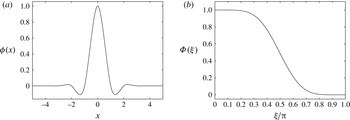
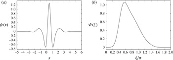
In the framework of the eddy-capturing approach, the separation between resolved flow structures and unresolved residual flow is obtained through a nonlinear multi-resolution wavelet thresholding filter (WTF), e.g. Goldstein & Vasilyev (Reference Goldstein and Vasilyev2004). The filtering operation is performed by applying the wavelet transform to the unfiltered velocity field, zeroing the wavelet coefficients below a given threshold, and transforming back to the physical space. In this study, the wavelet-filtered penalized perturbation velocity is formally represented (at a given time instant) by
 $$\begin{eqnarray}\overline{u}_{i}^{{>}{\it\epsilon}}(\boldsymbol{x})=\mathop{\sum }_{\boldsymbol{l}\in \mathscr{L}^{1}}c_{\boldsymbol{l}}^{1}{\it\phi}_{\boldsymbol{l}}^{1}(\boldsymbol{x})+\mathop{\sum }_{j=1}^{J}\mathop{\sum }_{{\it\mu}=1}^{2^{3}-1}\mathop{\sum }_{\stackrel{\boldsymbol{k}\in \mathscr{K}^{{\it\mu},j}}{|d_{\boldsymbol{k}}^{{\it\mu},j}|>{\it\epsilon}\Vert u_{i}(\boldsymbol{x})\Vert }}d_{\boldsymbol{k}}^{{\it\mu},j}{\it\psi}_{\boldsymbol{k}}^{{\it\mu},j}(\boldsymbol{x}),\end{eqnarray}$$
where
 ${\it\epsilon}$
stands for the non-dimensional thresholding level. The filtering process results in the decomposition of the velocity variable into two different parts, which are a coherent more energetic field and a residual less energetic coherent/incoherent one, say
 $u_{i}=\overline{u}_{i}^{{>}{\it\epsilon}}+u_{i}^{\prime }$
. In the wavelet decomposition (2.5), bold subscripts denote three-dimensional indices, while
 $\mathscr{L}^{1}$
and
 $\mathscr{K}^{{\it\mu},j}$
are three-dimensional index sets associated with scaling functions
 ${\it\phi}_{\boldsymbol{l}}^{1}$
and wavelets
 ${\it\psi}_{\boldsymbol{k}}^{{\it\mu},j}$
respectively. Each level of resolution
 $1\leqslant j\leqslant J$
(where
 $J$
is the maximum level present in the approximation) consists of multi-dimensional second-generation wavelets of the same family (indexed by
 ${\it\mu}$
), having the same scale, but located at different grid positions. As the wavelet decomposition (2.5) and the associated WTF procedure are central to the present computational methodology, a few more details are given in appendix A.
The momentum equations (2.2) are evaluated at collocation points, which leads to a set of nonlinear ordinary differential equations for the collocated velocity unknowns. The above wavelet decomposition is used for both grid adaptation and interpolation, while a hierarchical finite difference scheme, which takes advantage of the wavelet multilevel decomposition, is used for numerical differentiation (Vasilyev & Kevlahan Reference Vasilyev and Kevlahan2005). The multilevel structure of the wavelet approximation provides a natural way to obtain the solution on a near optimal grid. Due to the one-to-one correspondence between wavelets and grid points, the latter are omitted from the computational mesh if the associated wavelets are omitted from the representation (2.5), which occurs when the corresponding coefficients are below the given thresholding level. The method allows the numerical grid to dynamically adapt to the evolution of the flow structures, in both location and scale, while higher-resolution computations are conducted where and only where sharp gradients in the flow field occur.
Depending on the choice of the non-dimensional parameter
 ${\it\epsilon}$
, only a small fraction of the available wavelets are used in evolving the resolved velocity field
 $\overline{u}_{i}^{{>}{\it\epsilon}}$
, which results in the characteristic compression property of wavelet-based methods, e.g. Schneider & Vasilyev (Reference Schneider and Vasilyev2010). It should be mentioned that, during the grid adaptation process, once the wavelet mask is created for the collocation points associated with wavelets with significant coefficients, the same mask is extended by adding the adjacent wavelets, in both location and scale, whose coefficients can potentially become significant at the next time step. The use of the additional collocation points associated with adjacent wavelets causes a partial detriment of the grid compression, which, however, remains very high.
When combining the AWC approach with the volume-penalization technique discussed in the previous section, the presence of solid obstacles is automatically taken into account by the adaptive computational mesh. In this case, in addition to adapting on the resolved velocity field, the grid may also adapt on the discontinuous mask function
 ${\it\chi}_{s}$
. The AWC method is particularly effective in the simulation of external flows, because it has the ability to unambiguously identify and isolate localized dynamically dominant flow structures and to track them. Differently from the classical zonal mesh approach, where the numerical grid is a priori designed to resolve the main flow structures in the wake region, regardless of the instantaneous vorticity distribution, the wavelet-based adaptation allows the computational mesh to be continuously modified in time in order to automatically follow the evolution of the wake structure.
One of the main strengths of the present combined method lies in the direct control of the solution errors. On the one hand, the penalization error is regulated by the parameter
 ${\it\eta}$
, while, on the other hand, the numerical accuracy is controlled through the thresholding level
 ${\it\epsilon}$
in the wavelet decomposition (2.5). Therefore, the desired level of approximation can be achieved by appropriately prescribing these two parameters. It is worth stressing, however, that there exists a thin boundary layer inside the penalized region
 ${\it\Omega}_{s}$
, whose thickness is proportional to
 $({\it\eta}{\it\nu})^{1/2}$
, that needs to be resolved. The necessary numerical resolution thus increases with decrease of the obstacle porosity, which should be as low as possible to achieve the accurate estimation of the fluid–structure interaction force (2.4) (Mimeau et al.
Reference Mimeau, Gallizio, Cottet and Mortazavi2015). Hence, given the fluid viscosity, the thresholding level
 ${\it\epsilon}$
cannot be chosen independently from the penalty constant
 ${\it\eta}$
, but should decrease with it, in order to maintain the total simulation error to an a priori prescribed level (De Stefano & Vasilyev Reference De Stefano and Vasilyev2014). In fact, the automated wavelet-based grid adaptation guarantees the adequate resolution of the inner skin layer with the optimal grid compression, ensuring the required level of spatial accuracy without resorting to high-order methods that were recently proposed (Shirokoff & Nave Reference Shirokoff and Nave2015).
The choice of the threshold
 ${\it\epsilon}$
determines the relative energy level of the eddies that are resolved and, consequently, controls the importance of the residual field associated with the discarded wavelets. In principle, a very low but non-zero value for this parameter can be prescribed so that the effect of unresolved motions can be completely ignored and the direct solution of the governing equations (2.2) is provided. Even though the number of degrees of freedom is strongly reduced compared with non-adaptive DNS, and the Reynolds number scaling improves with respect to conventional estimates (Nejadmalayeri, Vezolainen & Vasilyev Reference Nejadmalayeri, Vezolainen and Vasilyev2013), the WDNS approach still remains unaffordable, even at moderately high Reynolds numbers.
2.3. Adaptive large-eddy simulation
The cost of the wavelet-based approach can be substantially reduced if higher thresholding levels are adopted. In this case, the influence of the residual (filtered out) motions on the dynamics of the resolved flow cannot be neglected and must be approximated by a closure model, resulting in the wavelet-based adaptive LES approach (Goldstein & Vasilyev Reference Goldstein and Vasilyev2004).
The interpretation of using the WTF procedure as an LES filter is actually twofold. First, the filtering process can be naturally interpreted from the energetic point of view. The decomposition (2.5) corresponds to the introduction of a velocity scale or, equivalently, a kinetic energy scale that reflects the turbulence resolution of the LES field. The characteristic turbulence resolution energy scale can be written as
 ${\it\epsilon}^{2}k$
, where
 $k=(u_{i}u_{i})/2$
is the kinetic energy associated with the unfiltered turbulent velocity field. Turbulent eddies with energies above this threshold are resolved, while the effect of less energetic eddies is modelled. Second, given the one-to-one correspondence between wavelet coefficients and grid points, the same procedure can be viewed as the implicit application of a low-pas non-uniform spatial filter. The characteristic turbulent resolution length scale, say
 ${\it\Delta}$
, can be practically evaluated knowing the position of the retained points on the AWC mesh. According to this interpretation, large-scale dynamically important flow structures are resolved, while the effect of small-scale residual motions is modelled. In this framework, the wavelet-based LES method resembles the classical LES procedure with non-uniform filtering, however with a fundamental difference. Namely, the non-uniform width of the LES filter induced by the WTF procedure is not prescribed but varies dynamically and continuously, while adapting to the flow evolution.
In this study, the governing equations for adaptive LES are formally obtained by applying the WTF operator (2.5) to the penalized momentum equations (2.2), followed by the divergence-free projection. This leads to the following equations in the unknown wavelet-filtered penalized perturbation velocity:
 $$\begin{eqnarray}\displaystyle & \displaystyle \frac{\partial \overline{u}_{i}^{{>}{\it\epsilon}}}{\partial x_{i}}=0, & \displaystyle\end{eqnarray}$$
 $$\begin{eqnarray}\displaystyle & \displaystyle \frac{\partial \overline{u}_{i}^{{>}{\it\epsilon}}}{\partial t}+(\overline{u}_{j}^{{>}{\it\epsilon}}+U_{j})\frac{\partial \overline{u}_{i}^{{>}{\it\epsilon}}}{\partial x_{j}}=-\frac{\partial \overline{P}^{{>}{\it\epsilon}}}{\partial x_{i}}+{\it\nu}\frac{\partial ^{2}\overline{u}_{i}^{{>}{\it\epsilon}}}{\partial x_{j}\partial x_{j}}-\frac{{\it\chi}_{s}}{{\it\eta}}(\overline{u}_{i}^{{>}{\it\epsilon}}+U_{i})-\frac{\partial {\it\tau}_{ij}}{\partial x_{j}}, & \displaystyle\end{eqnarray}$$
 ${\it\tau}_{ij}=\overline{u_{i}u_{j}}^{{>}{\it\epsilon}}-\overline{u}_{i}^{{>}{\it\epsilon}}\overline{u}_{j}^{{>}{\it\epsilon}}$
stand for the subgrid-scale (SGS) stresses that have to be modelled. It is worth noting that the bar used in the notation of the kinematic pressure variable
 $\overline{P}^{{>}{\it\epsilon}}$
does not imply the application of the WTF operator, but is used only for consistency with the other terms. Instead, the pressure term on the right-hand side of (2.7) must be viewed as a Lagrange multiplier enforcing the incompressibility constraint (2.6). Finally, it should be mentioned that, as happens for traditional non-adaptive LES with non-uniform filter width, there is a commutation error between filtering and derivative operators, which is not considered here. In fact, this error is significantly reduced by using the adjacent zone in the grid adaptation process (Schneider & Vasilyev Reference Schneider and Vasilyev2010).
3. Energy-based closure model
Different localized turbulence models that have been developed in the past for closing the wavelet-based LES equations in the context of homogeneous turbulence (De Stefano, Vasilyev & Goldstein Reference De Stefano, Vasilyev and Goldstein2008; Vasilyev et al. Reference Vasilyev, De Stefano, Goldstein and Kevlahan2008) can be used for the present inhomogeneous bluff-body flows. Here, the governing equations for the penalized adaptive LES approach are closed by means of a one-equation kinetic-energy-based model. Specifically, the residual deviatoric stresses (denoted by a star symbol) are approximated according to the eddy-viscosity assumption (Smagorinsky Reference Smagorinsky1963), that is,
 $$\begin{eqnarray}{\it\tau}_{ij}^{\ast }\cong -2{\it\nu}_{t}\overline{\unicode[STIX]{x1D61A}_{ij}}^{{>}{\it\epsilon}},\end{eqnarray}$$
where
 $\overline{\unicode[STIX]{x1D61A}}_{ij}^{{>}{\it\epsilon}}=((\partial \overline{u}_{i}^{{>}{\it\epsilon}}/\partial x_{j})+(\partial \overline{u}_{j}^{{>}{\it\epsilon}}/\partial x_{i}))/2$
is the resolved rate-of-strain tensor. The turbulent eddy viscosity is defined using the square root of the SGS turbulent kinetic energy,
 $k_{sgs}={\it\tau}_{ii}/2$
, as the velocity scale and the wavelet filter width
 ${\it\Delta}$
as the length scale,
 $$\begin{eqnarray}{\it\nu}_{t}(\boldsymbol{x},t)=C_{{\it\nu}}{\it\Delta}k_{sgs}^{1/2},\end{eqnarray}$$
where
 $C_{{\it\nu}}$
stands for a dimensionless model parameter to be determined. In this way, the model for the SGS stresses becomes
 $$\begin{eqnarray}{\it\tau}_{ij}\cong {\textstyle \frac{2}{3}}k_{sgs}{\it\delta}_{ij}-2C_{{\it\nu}}{\it\Delta}k_{sgs}^{1/2}\overline{\unicode[STIX]{x1D61A}_{ij}}^{{>}{\it\epsilon}},\end{eqnarray}$$
where
 ${\it\delta}_{ij}$
is the Kronecker delta. The SGS turbulent kinetic energy stands for a spatio-temporally evolving flow variable that reflects the local turbulence intensity. In fact, it represents an SGS quantity, although it is solved at the LES filter level. In order to close the LES governing equations (2.7), supplied with the model (3.3), an additional evolution equation for the SGS kinetic energy variable is derived as follows.
The balance equation for the kinetic energy associated with the unfiltered penalized perturbation velocity, which is obtained from the momentum equations (2.2), can be written as
 $$\begin{eqnarray}\frac{\partial k}{\partial t}+(u_{j}+U_{j})\frac{\partial k}{\partial x_{j}}=-u_{i}\frac{\partial P}{\partial x_{i}}+{\it\nu}\frac{\partial ^{2}k}{\partial x_{j}\partial x_{j}}-{\it\varepsilon}-\frac{{\it\chi}_{s}}{{\it\eta}}(2k+u_{i}U_{i}),\end{eqnarray}$$
where
 ${\it\varepsilon}={\it\nu}((\partial u_{i}/\partial x_{j})(\partial u_{i}/\partial x_{j}))$
stands for the so-called pseudo-dissipation (Pope Reference Pope2000). On the other hand, the balance equation for the kinetic energy associated with the resolved wavelet-filtered penalized perturbation velocity, say
 $k_{res}=(\overline{u}_{i}^{{>}{\it\epsilon}}\overline{u}_{i}^{{>}{\it\epsilon}})/2$
, which is obtained from the filtered momentum equations (2.7), can be written as
 $$\begin{eqnarray}\displaystyle \frac{\partial k_{res}}{\partial t}+(\overline{u}_{j}^{{>}{\it\epsilon}}+U_{j})\frac{\partial k_{res}}{\partial x_{j}} & = & \displaystyle -\overline{u}_{i}^{{>}{\it\epsilon}}\frac{\partial \overline{P}^{{>}{\it\epsilon}}}{\partial x_{i}}+{\it\nu}\frac{\partial ^{2}k_{res}}{\partial x_{j}\partial x_{j}}-{\it\varepsilon}_{res}\nonumber\\ \displaystyle & & \displaystyle -\,{\it\Pi}-\frac{\partial }{\partial x_{i}}(\overline{u}_{j}^{{>}{\it\epsilon}}{\it\tau}_{ij})-\frac{{\it\chi}_{s}}{{\it\eta}}(2k_{res}+\overline{u}_{i}^{{>}{\it\epsilon}}U_{i}),\end{eqnarray}$$
where
 ${\it\varepsilon}_{res}={\it\nu}((\partial \overline{u}_{i}^{{>}{\it\epsilon}}/\partial x_{j})(\partial \overline{u}_{i}^{{>}{\it\epsilon}}/\partial x_{j}))$
stands for the pseudo-dissipation of the resolved kinetic energy. The term
 ${\it\Pi}=-{\it\tau}_{ij}(\partial \overline{u}_{i}^{{>}{\it\epsilon}}/\partial x_{j})\equiv -{\it\tau}_{ij}\overline{\unicode[STIX]{x1D61A}}_{ij}^{{>}{\it\epsilon}}$
represents the SGS dissipation of the resolved kinetic energy, which is the rate at which energy is locally transferred from energetic resolved eddies to unresolved residual motions. Due to the eddy-viscosity model (3.1), this variable is approximated as
 ${\it\Pi}\cong {\it\nu}_{t}|\overline{\unicode[STIX]{x1D61A}}^{{>}{\it\epsilon}}\!|^{2}$
, where
 $|\overline{\unicode[STIX]{x1D61A}}^{{>}{\it\epsilon}}|=(2\overline{\unicode[STIX]{x1D61A}}_{ij}^{{>}{\it\epsilon}}\overline{\unicode[STIX]{x1D61A}}_{ij}^{{>}{\it\epsilon}})^{1/2}$
is the characteristic rate-of-strain magnitude. The SGS dissipation variable serves as a measure of the local turbulence resolution, that is, the level at which the most important turbulent eddies are resolved and the less important ones are modelled. It has been proven, both theoretically and empirically, that the amount of SGS dissipation in the wavelet-based LES approach increases with the thresholding level, e.g. Goldstein & Vasilyev (Reference Goldstein and Vasilyev2004).
Since the SGS turbulent kinetic energy is defined as the difference between the filtered kinetic energy and the kinetic energy of the filtered velocity field, that is,
 $$\begin{eqnarray}k_{sgs}={\textstyle \frac{1}{2}}\overline{u_{i}u_{i}}^{{>}{\it\epsilon}}-{\textstyle \frac{1}{2}}\overline{u}_{i}^{{>}{\it\epsilon}}\overline{u}_{i}^{{>}{\it\epsilon}}=\overline{k}^{{>}{\it\epsilon}}-k_{res},\end{eqnarray}$$
the corresponding balance equation can be achieved by filtering equation (3.4) and combining with (3.5), which provides
 $$\begin{eqnarray}\displaystyle \frac{\partial k_{sgs}}{\partial t}+(\overline{u}_{j}^{{>}{\it\epsilon}}+U_{j})\frac{\partial k_{sgs}}{\partial x_{j}} & = & \displaystyle {\it\nu}\frac{\partial ^{2}k_{sgs}}{\partial x_{j}\partial x_{j}}-\frac{\partial }{\partial x_{i}}(\overline{u_{i}P}^{{>}{\it\epsilon}}-\overline{u}_{i}^{{>}{\it\epsilon}}\overline{P}^{{>}{\it\epsilon}})-{\it\varepsilon}_{sgs}\nonumber\\ \displaystyle & & \displaystyle +\,{\it\Pi}+\frac{\partial }{\partial x_{i}}(\overline{u}_{j}^{{>}{\it\epsilon}}{\it\tau}_{ij})-\frac{{\it\chi}_{s}}{{\it\eta}}(2k_{sgs}).\end{eqnarray}$$
The variable
 ${\it\Pi}$
, which appears with opposite sign in (3.5) and (3.7), represents here the production of SGS energy due to interaction between resolved and residual motions. The variable
 ${\it\varepsilon}_{sgs}$
stands for the unknown dissipation rate of SGS energy,
 $$\begin{eqnarray}{\it\varepsilon}_{sgs}={\it\nu}\left(\overline{\frac{\partial u_{i}}{\partial x_{j}}\frac{\partial u_{i}}{\partial x_{j}}}^{{>}{\it\epsilon}}-\frac{\partial \overline{u}_{i}^{{>}{\it\epsilon}}}{\partial x_{j}}\frac{\partial \overline{u}_{i}^{{>}{\it\epsilon}}}{\partial x_{j}}\right)=\overline{{\it\varepsilon}}^{{>}{\it\epsilon}}-{\it\varepsilon}_{res},\end{eqnarray}$$
which needs to be modelled. In this work, according to simple scaling arguments, the following approximation is used:
 $$\begin{eqnarray}{\it\varepsilon}_{sgs}(\boldsymbol{x},t)\cong C_{{\it\varepsilon}}k_{sgs}^{3/2}/{\it\Delta},\end{eqnarray}$$
where
 $C_{{\it\varepsilon}}$
stands for the second dimensionless model parameter to be determined.
As is commonly done for energy-based LES methods, the residual unclosed terms on the right-hand side of (3.7) are modelled by the local diffusion of SGS energy due to turbulent eddy viscosity, without making further modelling assumptions, e.g. Ghosal et al. (Reference Ghosal, Lund, Moin and Akselvoll1995). In this way, the transport model equation for the SGS turbulent kinetic energy to be actually solved becomes
 $$\begin{eqnarray}\frac{\partial k_{sgs}}{\partial t}+(\overline{u}_{j}^{{>}{\it\epsilon}}+U_{j})\frac{\partial k_{sgs}}{\partial x_{j}}=\frac{\partial }{\partial x_{j}}\left[({\it\nu}+{\it\nu}_{t})\frac{\partial k_{sgs}}{\partial x_{j}}\right]-{\it\varepsilon}_{sgs}+{\it\Pi}-\frac{2{\it\chi}_{s}}{{\it\eta}}k_{sgs}.\end{eqnarray}$$
It is worth noting that the variable
 $k_{sgs}$
is penalized in such a way that it vanishes inside the volume occupied by the solid obstacle. This fact leads to the introduction of the additional penalty term in (3.10) with respect to the original wavelet-based formulation for homogeneous turbulent flows (De Stefano et al.
Reference De Stefano, Vasilyev and Goldstein2008; De Stefano & Vasilyev Reference De Stefano and Vasilyev2010). The SGS energy equation is solved together with the filtered momentum equations (2.7), with the associated incompressibility constraint (2.6), using the AWC solver.
The overall closure process, thus, involves the two model parameters
 $C_{{\it\nu}}$
and
 $C_{{\it\varepsilon}}$
, which can be either prescribed as constants or dynamically obtained as part of the solution. In this study, these coefficients are determined as space–time functions by means of a Germano-like dynamic procedure (Germano et al.
Reference Germano, Piomelli, Moin and Cabot1991). Following a classical approach, e.g. Liu, Meneveau & Katz (Reference Liu, Meneveau and Katz1994), an explicit low-pass spatial filter operation with width
 $\widehat{{\it\Delta}}=2{\it\Delta}$
is applied to the resolved velocity field, which leads to the definition of the test-filtered velocity. Due to the underlying scale-similarity assumption, information available from the resolved scales is utilized to set the unknown model parameters. The details of the dynamic procedure for establishing the localized energy-based model coefficients are given in appendix B.
It is worth stressing that the present LES closure model allows for negative values of the eddy-viscosity coefficient
 $C_{{\it\nu}}$
, thus accounting for local energy backscatter from SGS to resolved motions (
 ${\it\nu}_{t}<0$
). In a practical computation, however, the eddy-viscosity coefficient is clipped so as to ensure that
 ${\it\nu}+{\it\nu}_{t}\geqslant 0$
, consistently with the use of the total viscosity as the diffusion coefficient in the SGS energy equation (3.10). In fact, such a partial clipping procedure is quite common when using dynamic eddy-viscosity models that allow for energy backscatter, because it favourably affects the stability of the numerical calculation, e.g. Ghosal et al. (Reference Ghosal, Lund, Moin and Akselvoll1995).
Analogous energy-based one-equation models, where the dynamic evaluation of the model coefficients is based on either a Germano-like (Germano et al. Reference Germano, Piomelli, Moin and Cabot1991) or a Bardina-like (Bardina, Ferziger & Reynolds Reference Bardina, Ferziger and Reynolds1980) approach, have been successfully used for the non-adaptive finite-volume-based LES of bluff-body flows by Sohankar, Davidson & Norberg (Reference Sohankar, Davidson and Norberg2000), Krajnović & Davidson (Reference Krajnović and Davidson2002) and Fureby et al. (Reference Fureby, Alin, Wikström, Menon, Svanstedt and Persson2004).
4. Variable thresholding
In the wavelet-based adaptive LES approach that relies on the multi-resolution WTF approximation (2.5), both the numerical grid spacing and the LES filter width are continuously adapted on the solution. In the present study, the same wavelet thresholding level is used for both the AWC solver and the turbulence model, since it was demonstrated that the use of the explicit filtering formulation with two different levels of thresholding is not optimal (De Stefano & Vasilyev Reference De Stefano and Vasilyev2013). In its original formulation, the method uses a constant threshold parameter that is defined a priori, and, thus, the effective wavelet filter width
 ${\it\Delta}$
, which represents the local measure of both the numerical and the LES spatial resolution of the solution, is only somewhat controlled.
For homogeneous turbulent flows, this limitation has been partly removed in De Stefano & Vasilyev (Reference De Stefano and Vasilyev2012), where a time-varying thresholding method was proposed and successfully tested for both freely decaying and forced isotropic turbulence. The threshold variable was evolved in time according to a simple feedback control equation based on the ratio of volume-averaged modelled and resolved dissipations, which represents an objective physics-based measure of the LES resolution. Namely, the filtering operation (2.5) was performed with a level of thresholding
 ${\it\epsilon}={\it\epsilon}(t)$
, which was spatially uniform but dependent on the instantaneous level of resolved/modelled dissipation.
A more general variable thresholding formulation that includes spatial variation was recently considered and demonstrated for homogeneous isotropic turbulence by Nejadmalayeri et al. (Reference Nejadmalayeri, Vezolainen, De Stefano and Vasilyev2014). In the present work, the spatio-temporally varying thresholding is extended to wall-bounded flows, while formalizing the approach in the framework of the Lagrangian path-line diffusive averaging methodology (Vasilyev et al. Reference Vasilyev, De Stefano, Goldstein and Kevlahan2008).
4.1. Lagrangian path-line diffusive averaged threshold
The threshold parameter in the wavelet decomposition (2.5) does not need to be constant but may actually vary. The space–time variability of the wavelet threshold can be exploited to implement a physics-based coupling between the computational grid and the turbulence modelling that ensures the uniform desired fidelity of the numerical simulations. The main idea is to continuously adjust the threshold variable by monitoring a suitable measure of the local turbulence resolution and providing a feedback that influences the evolution of the threshold field. At the same time, the threshold variation should be sufficiently smooth in order not to lead to the appearance of unphysical small scales in the velocity field. In order to avoid this undesirable behaviour, the wavelet threshold should change in accordance with the local flow evolution on a time scale corresponding to the local time scale of the flow.
One way to impose a fair level of variability is to use the following integral threshold:
 $$\begin{eqnarray}\mathscr{I}_{{\it\epsilon}}(\boldsymbol{x},t)=\frac{1}{{\it\tau}_{{\it\epsilon}}}\int _{-\infty }^{t}\text{e}^{-((t-t^{\prime })/{\it\tau}_{{\it\epsilon}})}{\it\epsilon}(\boldsymbol{x}(t^{\prime }),t^{\prime })\,\text{d}t^{\prime },\end{eqnarray}$$
resulting from exponentially weighted time averaging along the trajectory of a fluid particle, where the variable
 ${\it\tau}_{{\it\epsilon}}$
stands for a relaxation time parameter. By differentiating (4.1) with respect to time, the following evolution equation for the Lagrangian path-line-averaged threshold is obtained:
 $$\begin{eqnarray}\frac{\partial \mathscr{I}_{{\it\epsilon}}}{\partial t}+(\overline{u}_{i}^{{>}{\it\epsilon}}+U_{i})\frac{\partial \mathscr{I}_{{\it\epsilon}}}{\partial x_{i}}=\frac{\mathscr{I}_{{\it\epsilon}}}{{\it\tau}_{{\it\epsilon}}}\left(\frac{{\it\epsilon}}{\mathscr{I}_{{\it\epsilon}}}-1\right),\end{eqnarray}$$
where
 ${\it\epsilon}={\it\epsilon}(\boldsymbol{x},t)$
represents the instantaneous threshold value to be achieved. The variable on the right-hand side of this equation can be interpreted as a forcing term, say
 $f_{{\it\epsilon}}$
, that forces the threshold evolution so that the difference
 $({\it\epsilon}-\mathscr{I}_{{\it\epsilon}})$
asymptotically tends to vanish.
Here, the local adjustment of the wavelet threshold is obtained through the application of a physics-based, spatially and temporally varying, forcing mechanism that is designed to locally maintain the desired level of turbulence resolution. The latter is measured by the ratio between the modelled SGS and the resolved viscous dissipations, that is,
 $$\begin{eqnarray}\mathscr{R}(\boldsymbol{x},t)=\frac{{\it\Pi}}{D},\end{eqnarray}$$
where
 $D={\it\nu}|\overline{\unicode[STIX]{x1D61A}}^{{>}{\it\epsilon}}|^{2}$
. This variable reflects the level at which the most energetic structures are resolved, while modelling the effect of residual unresolved motions. By exploiting the model (3.1), the monitor variable
 $\mathscr{R}$
is equivalently expressed as the ratio of eddy viscosity to molecular viscosity,
 $\mathscr{R}={\it\nu}_{t}/{\it\nu}$
. Previous wavelet-based LES studies have demonstrated that this ratio increases with the WTF level, specifically, being proportional to
 ${\it\epsilon}^{2}$
(Goldstein, Kevlahan & Vasilyev Reference Goldstein, Kevlahan and Vasilyev2005). In fact, the importance of the energy transfer (back and forth) between resolved and unresolved eddies is dictated by the thresholding factor that is actually used in the WTF definition (2.5). The basic idea is to exploit this correspondence by locally varying the threshold wherever the level of turbulent resolution, as measured by the field variable
 $\mathscr{R}$
, deviates from a given positive goal magnitude, say
 $\mathscr{R}_{goal}$
, which is a priori prescribed.
In this study, the forcing term on the right-hand side of the Lagrangian transport equation (4.2) is defined in terms of the turbulence resolution measure in such a way that
 $\mathscr{R}$
tends to
 $\mathscr{R}_{goal}$
for
 $\mathscr{I}_{{\it\epsilon}}$
approaching the desired threshold
 ${\it\epsilon}$
. Due to the abovementioned quadratic dependence, it can be assumed that
 $\mathscr{R}_{goal}/\mathscr{R}\sim {\it\epsilon}^{2}/\mathscr{I}_{{\it\epsilon}}^{2}$
, resulting in the following forcing scheme in the regions of forward scatter (
 $\mathscr{R}>0$
):
 $$\begin{eqnarray}f_{{\it\epsilon}}(\boldsymbol{x},t)=\frac{\mathscr{I}_{{\it\epsilon}}}{{\it\tau}_{{\it\epsilon}}}\left(\sqrt{\frac{\mathscr{R}_{goal}}{\mathscr{R}}}-1\right).\end{eqnarray}$$
In this way, given the desired level of turbulence resolution, determined by the user-defined parameter
 $\mathscr{R}_{goal}$
, the two-way feedback mechanism between the physical resolution of the LES field and the numerical resolution of the computational mesh works as follows. In flow regions of relatively low turbulence resolution, where
 $\mathscr{R}>\mathscr{R}_{goal}$
, the thresholding variable is forced to diminish (
 $f_{{\it\epsilon}}<0$
), which leads to local mesh refining, with subsequent growth of the resolved viscous dissipation and reduction of the SGS dissipation to be modelled. On the contrary, in regions of relatively high resolution, where
 $0<\mathscr{R}<\mathscr{R}_{goal}$
, the threshold is forced to augment (
 $f_{{\it\epsilon}}>0$
), which leads to mesh coarsening, with subsequent decrease of the resolved dissipation and increase of the SGS dissipation.
The relaxation time scale
 ${\it\tau}_{{\it\epsilon}}$
in (4.2) is a crucial parameter that determines how quickly the solution adjusts to local changes in the flow field. As found by De Stefano & Vasilyev (Reference De Stefano and Vasilyev2012), a physically motivated choice consists in employing the time scale associated with the characteristic rate of strain, namely,
 ${\it\tau}_{{\it\epsilon}}(\boldsymbol{x},t)=|\overline{\unicode[STIX]{x1D61A}}^{{>}{\it\epsilon}}\!|^{-1}$
. By using this time scale in the definition (4.4) and rearranging the right-hand side the following forcing scheme is obtained:
 $$\begin{eqnarray}f_{{\it\epsilon}}(\boldsymbol{x},t)=\frac{\mathscr{H}({\it\Pi})}{\sqrt{{\it\nu}}\sqrt{\mathscr{R}}}\left(\sqrt{\mathscr{R}_{goal}}\sqrt{D}-\sqrt{{\it\Pi}}\right)\mathscr{I}_{{\it\epsilon}},\end{eqnarray}$$
where the Heaviside function
 $\mathscr{H}(\cdot )$
ensures the desired behaviour in locations where backscatter occurs. In fact, the proposed forcing scheme, being based on the amount of modelled SGS dissipation compared with viscous dissipation, inherently relies on positive values of
 ${\it\Pi}$
and loses meaning in the presence of energy backscatter, where it is switched off. The use of the variable
 $\mathscr{R}$
in the forcing definition is undesirable because of its high variability and possible singular behaviour in laminar or transitional flow regions. Also motivated by the fact that in the turbulent regions with forward scatter the turbulence resolution should approach the desired goal value,
 $\mathscr{R}$
can be replaced by
 $\mathscr{R}_{goal}$
in the above equation, which results in the following definition:
 $$\begin{eqnarray}f_{{\it\epsilon}}^{T}(\boldsymbol{x},t)=\frac{\mathscr{H}({\it\Pi})}{\sqrt{{\it\nu}}\sqrt{\mathscr{R}_{goal}}}\left(\sqrt{\mathscr{R}_{goal}}\sqrt{D}-\sqrt{{\it\Pi}}\right)\mathscr{I}_{{\it\epsilon}}.\end{eqnarray}$$
The superscript
 $T$
is applied here to highlight that this forcing scheme is inherently designed to be used in turbulent flow regions.
When practically solving the threshold evolution equation (4.2), supplied with the forcing (4.6), an artificial diffusion term needs to be added on the right-hand side in order to prevent the creation of high-frequency modes in the threshold field. These modes, which stem from intermittent turbulent fluctuations as well as aliasing errors, due to the AWC solver which automatically increases the numerical resolution where/when it is necessary, would otherwise cause deterioration of the grid compression. The resulting Lagrangian path-line diffusive averaging approach guarantees the smoothness of the spatially variable threshold and allows the consequential undesired small-scale fluctuations in the velocity field to be avoided. Also considering the physical diffusion due to the fluid viscosity, the evolution equation for the Lagrangian-averaged thresholding variable that is actually solved becomes
 $$\begin{eqnarray}\frac{\partial \mathscr{I}_{{\it\epsilon}}}{\partial t}+(\overline{u}_{i}^{{>}{\it\epsilon}}+U_{i})\frac{\partial \mathscr{I}_{{\it\epsilon}}}{\partial x_{i}}=\frac{\partial }{\partial x_{i}}\left[({\it\nu}+{\it\nu}_{{\it\epsilon}})\frac{\partial \mathscr{I}_{{\it\epsilon}}}{\partial x_{i}}\right]+f_{{\it\epsilon}},\end{eqnarray}$$
where
 $f_{{\it\epsilon}}=f_{{\it\epsilon}}^{T}(\boldsymbol{x},t)$
. The viscosity-like coefficient
 ${\it\nu}_{{\it\epsilon}}$
for the artificial diffusion term is determined by imposing that the diffusion time scale
 ${\it\Delta}^{2}/{\it\nu}_{{\it\epsilon}}$
is comparable to the local time scale
 $|\overline{\unicode[STIX]{x1D61A}}^{{>}{\it\epsilon}}\!|^{-1}$
. This leads to utilizing the classical Smagorinsky-like scaling for this parameter, namely,
 ${\it\nu}_{{\it\epsilon}}(\boldsymbol{x},t)=C_{{\it\nu}_{{\it\epsilon}}}{\it\Delta}^{2}|\overline{\unicode[STIX]{x1D61A}}^{{>}{\it\epsilon}}\!|$
, where
 $C_{{\it\nu}_{{\it\epsilon}}}$
is a dimensionless coefficient of order unity (Nejadmalayeri et al.
Reference Nejadmalayeri, Vezolainen, De Stefano and Vasilyev2014).
The evolution equation (4.7) provides the pointwise time-dependent thresholding level that is actually used during the computation for both the AWC numerical method and the adaptive LES filtering. However, the threshold variable must be bounded from both below, to avoid too low thresholds corresponding to the CVS and WDNS regimes, and above, to prevent too high thresholds that would reduce the numerical accuracy of the solution. Finally, it is worth stressing that the proposed variable thresholding method is totally independent of the closure model that is utilized for approximating the SGS dissipation.
4.2. Bluff-body flows
For inhomogeneous bluff-body flows it is necessary to enhance the above varying thresholding strategy with additional considerations that lead to modification of the forcing term on the right-hand side of the evolution equation (4.7). First, in the regions of undisturbed laminar flow, away from the obstacle, both the resolved and the SGS dissipations are negligible and, thus, the forcing (4.6) would not practically affect the solution. In order to save computational resources, in these regions the threshold field should instead approach the maximum allowable value, which is chosen compatibly with the necessary numerical accuracy. To enforce this desired trend, the following additional forcing term is considered:
 $$\begin{eqnarray}f_{{\it\epsilon}}^{L}(\boldsymbol{x},t)=\max \left(\frac{U}{H}-A,0\right)\mathscr{I}_{{\it\epsilon}},\end{eqnarray}$$
where
 $H$
stands for the characteristic linear extent of the body and
 $A$
represents the norm of the velocity-gradient tensor
 $\overline{\unicode[STIX]{x1D608}}_{ij}^{{>}{\it\epsilon}}=\overline{\unicode[STIX]{x1D61A}}_{ij}^{{>}{\it\epsilon}}+\overline{{\it\Omega}}_{ij}^{{>}{\it\epsilon}}$
, with
 $\overline{{\it\Omega}}_{ij}^{{>}{\it\epsilon}}=((\partial \overline{u}_{i}^{{>}{\it\epsilon}}/\partial x_{j})-(\partial \overline{u}_{j}^{{>}{\it\epsilon}}/\partial x_{i}))/2$
being the resolved rate-of-rotation tensor. The superscript
 $L$
is applied here to highlight that this forcing scheme is dominant in laminar flow regions. In fact,
 $f_{{\it\epsilon}}^{L}$
is effective only in the undisturbed flow regions, where
 $A<U/H$
, on the convective time scale
 $H/U$
, while being null in both the near-wall and wake regions, where
 $A>U/H$
, as empirically confirmed by the results of the present numerical experiments.
In addition, it should be noted that the forcing term (4.6) does not exhibit the right limiting behaviour when approaching the obstacle surface. In fact, since the modelled SGS dissipation vanishes at the wall, whereas the resolved viscous dissipation does not, the wavelet threshold would tend towards the upper bound of the admissible range. This trend is undesirable because the use of relatively large thresholds in the near-wall region would decrease the local numerical accuracy, whereas it should be increased. For this reason, there the forcing
 $f_{{\it\epsilon}}^{T}$
should be switched off, while an alternative forcing term of opposite sign should be enforced. One of the possible mechanisms for achieving the right forcing change is based on the local turbulence intensity, which is measured by the ratio of SGS and free-stream kinetic energies. In the flow regions where the turbulent intensity is below a given low level, say
 $k_{sgs}<{\it\alpha}U^{2}/2$
, with
 ${\it\alpha}\ll 1$
, the forcing (4.6) is switched off, while being replaced by
 $$\begin{eqnarray}f_{{\it\epsilon}}^{W}(\boldsymbol{x},t)=-\frac{U}{H}\mathscr{H}\left(A-\frac{U}{H}\right)\mathscr{I}_{{\it\epsilon}}.\end{eqnarray}$$
The Heaviside term on the right-hand side of this equation ensures that
 $f_{{\it\epsilon}}^{W}$
is not effective in the regions of undisturbed flow, where
 $A<U/H$
, so that it does not alter the previous forcing mechanism based on (4.8). The superscript
 $W$
is applied here to highlight that this forcing scheme is active in both the near-wall and wake regions.
Finally, combination of all of these asymptotic mechanisms yields the following compounded forcing scheme:
 $$\begin{eqnarray}f_{{\it\epsilon}}(\boldsymbol{x},t)=\mathscr{H}\left(k_{sgs}-{\it\alpha}\frac{U^{2}}{2}\right)f_{{\it\epsilon}}^{T}+f_{{\it\epsilon}}^{L}+\mathscr{H}\left({\it\alpha}\frac{U^{2}}{2}-k_{sgs}\right)f_{{\it\epsilon}}^{W},\end{eqnarray}$$
which is valid in the entire fluid region.
It is worth noting that the proposed forcing scheme is suited to the case of an isolated bluff body. However, the method can be generalized to the case of multiple interacting bodies. Given and knowing the size and shape of the
 $i$
th obstacle, the associated characteristic linear extent, say
 $H_{i}$
, is defined. While leaving
 $f_{{\it\epsilon}}^{T}$
unaltered, the forcing functions
 $f_{{\it\epsilon}}^{L}$
and
 $f_{{\it\epsilon}}^{W}$
need to be modified so as to account for the simultaneous existence of the different convective time scales
 $H_{i}/U$
in the flow field. The parameter
 $H$
in the definition (4.8) can be substituted by the maximum length among the various
 $H_{i}$
, while the same parameter in (4.9) can be replaced by the minimum characteristic length.
The threshold evolution equation (4.7) is solved in the fluid domain
 ${\it\Omega}_{f}$
, supplied with the composite forcing term (4.10). According to the coupled wavelet-collocation/volume-penalization approach, the solution of an additional evolution equation for the unknown variable
 $\mathscr{I}_{{\it\epsilon}}$
in the obstacle domain
 ${\it\Omega}_{s}$
is required. In this study, a parabolic diffusion equation with a large diffusion coefficient is used, which ensures the smoothness of the wavelet threshold variable inside the penalized region. In this way, combining this latter equation with (4.7) and employing the mask function definition (2.3), the overall evolution equation for the variable thresholding level becomes
 $$\begin{eqnarray}\frac{\partial \mathscr{I}_{{\it\epsilon}}}{\partial t}+(\overline{u}_{i}^{{>}{\it\epsilon}}+U_{i})\frac{\partial \mathscr{I}_{{\it\epsilon}}}{\partial x_{i}}=(1-{\it\chi}_{s})\left\{\frac{\partial }{\partial x_{i}}\left[({\it\nu}+{\it\nu}_{{\it\epsilon}})\frac{\partial \mathscr{I}_{{\it\epsilon}}}{\partial x_{i}}\right]+f_{{\it\epsilon}}\right\}+{\it\chi}_{s}\mathscr{D}\frac{\partial ^{2}\mathscr{I}_{{\it\epsilon}}}{\partial x_{i}\partial x_{i}}.\end{eqnarray}$$
The actual diffusive strength of the last term on the right-hand side of this equation is determined based upon a numerical stability constraint, which results in choosing
 $\mathscr{D}>{\it\delta}^{2}/{\it\eta}$
, where
 ${\it\delta}$
is the local spatial resolution inside the penalty region.
5. Numerical experiments
The combined wavelet-collocation/volume-penalization method is applied to the simulation of the incompressible flow around a stationary right prism with square cross-section, immersed in a uniform fluid stream. The sharp edges of the body, which has one side facing the oncoming flow, determine where the flow separations take place, which minimizes the influence of the inlet boundary conditions. The mean flow Reynolds number is
 $Re=UH/{\it\nu}=2000$
, where
 $H$
corresponds to the side length of the cylinder cross-section. As expected for this supercritical Reynolds number, the separating shear layers on both sides of the cylinder are observed to become unstable and the complete transition to turbulent flow occurs (Lyn & Rodi Reference Lyn and Rodi1994; Lyn et al.
Reference Lyn, Einav, Rodi and Park1995).
5.1. Case settings
The flow around the two-dimensional obstacle is described in a Cartesian coordinate system
 $(x,y,z)$
, where the
 $x$
-axis corresponds to the inlet flow direction and the
 $z$
-axis coincides with the symmetry axis of the cylinder. Moreover, the square cross-section is aligned with the first two coordinate directions. The computational domain is defined by
 ${\it\Omega}=[-x_{in},x_{out}]\times [-a/2,a/2]\times [-b/2,b/2]$
, where
 $a$
and
 $b$
represent the lateral and spanwise extents respectively, while the domain occupied by the immersed body is
 ${\it\Omega}_{s}=[-H/2,H/2]\times [-H/2,H/2]\times [-b/2,b/2]$
. The non-dimensional lateral extent of the domain defines the solid blockage ratio, that is,
 ${\it\beta}=H/a$
, which measures the actual confinement of the flow. For the numerical experiments that are presented in the following, the spanwise and the lateral extents are
 $b=4H$
and
 $a=16H$
respectively, while the streamwise extent is determined by fixing
 $x_{in}=6H$
and
 $x_{out}=18H$
. The moderate length-to-width ratio of the square cylinder allows for simulating the evolution of three-dimensional flow structures in the spanwise homogeneity direction, while saving computational resources.
The filtered penalized momentum equations (2.7) are solved in
 ${\it\Omega}$
, supplied with the following boundary conditions for the unknown perturbation velocity field: zero-velocity conditions imposed at the inflow boundary (
 $x=-x_{in}$
), convective conditions prescribed at the outflow boundary (
 $x=x_{out}$
), free-slip conditions set at the lateral boundaries (
 $y=\pm a/2$
), specifically
 $\partial \overline{u}_{1}^{{>}{\it\epsilon}}/\partial y=\overline{u}_{2}^{{>}{\it\epsilon}}=\partial \overline{u}_{3}^{{>}{\it\epsilon}}/\partial y=0$
, and periodic conditions assumed in the spanwise direction (
 $z=\pm b/2$
). The no-slip boundary condition at the fluid–body interface is imposed by setting
 $\bar{{\it\eta}}={\it\eta}U/H=5\times 10^{-4}$
as the non-dimensional penalization coefficient. This choice represents a good compromise between the need to accurately simulate the fluid–structure interaction and the need to achieve a reasonable computational cost.
As far as the energy transport equation (3.10) is concerned, the SGS turbulent kinetic energy variable is evolved starting from a uniform very low but non-zero value, namely,
 $k_{0}=10^{-8}U^{2}$
. In this way, the initial turbulence level is practically negligible, which introduces a certain difference with respect to the reference experimental studies, e.g. Lyn et al. (Reference Lyn, Einav, Rodi and Park1995). For the boundary conditions, homogeneous Neumann conditions are enforced at the lateral boundaries and periodicity is assumed in the spanwise direction. Moreover, the steady level
 $k_{0}$
is maintained at the inflow boundary and convective conditions are set at the outflow boundary.
The numerical solutions have been obtained by employing the fourth-order AWC method, the linearized Crank–Nicolson split-step time-integration method with adaptive time stepping and the parallel version of the AWC solver (Nejadmalayeri et al.
Reference Nejadmalayeri, Vezolainen, Brown-Dymkoski and Vasilyev2015). The spatial discretization of the computational domain
 ${\it\Omega}$
is achieved by employing eight nested wavelet-collocation grids for the wavelet decomposition (2.5), where
 $J=8$
. The non-adaptive mesh spacings associated with the
 $j$
th grid are
 ${\rm\Delta}x^{j}={\rm\Delta}y^{j}={\it\delta}_{j}$
and
 ${\rm\Delta}z^{j}=2{\it\delta}_{j}$
, where
 ${\it\delta}_{j}=2^{-j+1}H$
, for
 $1\leqslant j\leqslant 8$
. In practice, as the three lower levels of resolution are kept all over the computational domain, the minimum and maximum spatial resolutions correspond to
 $({\rm\Delta}x,{\rm\Delta}y,{\rm\Delta}z)=(H/4,H/4,H/2)$
and
 $(H/128,H/128,H/64)$
respectively. The range of mesh sizes in the
 $(x,y)$
plane is similar to that involved in other LES studies of square cylinder flow, e.g. Sohankar et al. (Reference Sohankar, Davidson and Norberg2000) and Brun et al. (Reference Brun, Aubrun, Goossens and Ravier2008). Differently, the present spatial resolution in the spanwise direction is much higher than that adopted in these works. In particular, the spanwise resolution
 ${\rm\Delta}z/H=2/9$
of the LES solution at the same Reynolds number,
 $Re=2000$
, as presented in Brun et al. (Reference Brun, Aubrun, Goossens and Ravier2008) is undoubtedly low, whereas the present simulations appear to be over-resolved in the spanwise direction. This over-resolution is due to the homogeneous refinement intrinsic to wavelet-based methods combined with the necessity to have non-stretched mesh elements in the wake region.
It is worth stressing that, differently from other non-adaptive numerical studies, where the non-uniform mesh spacing in the
 $(x,y)$
plane is given a priori, according to a prescribed stretching law, while the grid in the spanwise direction is kept constant, in the present work, the actual grid is dynamically determined following the flow evolution in all three spatial dimensions. Even including the wavelets belonging to the adjacent zone, the actual mesh involves approximately 1 % of the total number of available wavelets. Thus, the grid compression remains very high, as typically happens for wavelet-based methods. Regarding computational cost, when making a fair comparison with classical non-adaptive methods, the additional cost of adaptation per point, which is between three and five times higher, must be taken into account. In this way, because more than 80 % of collocation points are discarded in the practical calculations, the present adaptive simulations can be considered to be more efficient than traditional non-adaptive ones.
As discussed in § 2.3, the volume-penalization approach results in the existence of a thin boundary layer inside the obstacle region with a non-dimensional thickness of order
 $(\bar{{\it\eta}}/Re)^{1/2}$
(Carbou & Fabrie Reference Carbou and Fabrie2003), which must be resolved. This requirement, combined with the isotropic wavelet refinement strategy that is currently adopted, results in substantially increasing the computational cost of the present simulations. This drawback will be addressed in the future with the use of the anisotropic wavelet transform that is currently under development. It should be noted that, due to the moderate Reynolds number, the present maximum resolution, namely
 ${\it\delta}_{8}/H=1/128$
is fully adequate to resolve the kinematic boundary layer inside the fluid region, whose non-dimensional thickness scales with
 $Re^{-1/2}$
. In fact, differently from attached boundary layer flows, where the turbulence production is essentially due to the fluid–wall interaction, here, the most important contribution to turbulence production is due to the flapping shear layers separating from the leading edges of the square cylinder and is associated with scales whose size is of the order of the shear layer thickness. Therefore, the spatial resolution constraint for wall-bounded flows can be partially relaxed and the present approach can be referred to as wall-resolved adaptive wavelet-based LES.
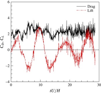
According to (2.4), the unsteady aerodynamic forces arising from fluid–structure interaction are expressed in terms of the following time-dependent spanwise-averaged drag and lift coefficients:
 $$\begin{eqnarray}C_{D}(t)\equiv \frac{F_{1}/(bH)}{\frac{1}{2}{\it\rho}U^{2}H}=\frac{2}{\bar{{\it\eta}}bH^{3}U}\int _{{\it\Omega}_{s}}(U+\overline{u}_{1}^{{>}{\it\epsilon}})\,\text{d}\boldsymbol{x}\end{eqnarray}$$
and
 $$\begin{eqnarray}C_{L}(t)\equiv \frac{F_{2}/(bH)}{\frac{1}{2}{\it\rho}U^{2}H}=\frac{2}{\bar{{\it\eta}}bH^{3}U}\int _{{\it\Omega}_{s}}\overline{u}_{2}^{{>}{\it\epsilon}}\,\text{d}\boldsymbol{x}\end{eqnarray}$$
respectively. In the following, the mean and the associated root mean square (r.m.s.) values of these variables are used as global quantities characterizing the numerical solution.
5.2. Results
The wavelet-based adaptive LES solution of square cylinder flow at
 $Re=2000$
is initially obtained by using the AWC solver with a uniform thresholding level. Due to its built-in dual nature, the choice of this parameter is not trivial. Indeed, the prescribed level must be sufficiently low in order to ensure adequate numerical accuracy but, at the same time, sufficiently high in order to achieve a certain turbulence resolution for the LES approach. A fair compromise between these two opposite requirements is pursued here by referring to previous studies and carrying out some preliminary experiments with different thresholds, which results in choosing the value
 ${\it\epsilon}=0.11$
. This thresholding level has also been proven to ensure the right wall resolution for the given value of
 $\bar{{\it\eta}}$
. In fact, the accuracy with which the no-slip wall-boundary condition is imposed unavoidably affects the choice of the thresholding level, which must decrease with the penalization parameter (De Stefano & Vasilyev Reference De Stefano and Vasilyev2014).
Time histories of the spanwise-averaged drag and lift coefficients.

The numerical solution is obtained starting from zero perturbation velocity as initial condition and conducting the computation until the wake is fully developed and quasi-periodical vortex shedding occurs. The incoming flow is undisturbed and the wake transitional process is naturally promoted by the numerical truncation errors. After a transient period, during which the wake develops from initial free-stream conditions, the aerodynamic forces exhibit the classical quasi-oscillatory behaviour of bluff-body flows. This is illustrated in figure 1, where the time histories of the spanwise-averaged drag and lift coefficients are reported for approximately four shedding cycles. It should be mentioned that the present value of
 $\bar{{\it\eta}}$
, which affects the simulation of the fluid–structure interaction, could be responsible for non-physical oscillations in the time-dependent force coefficients. However, it is believed to have a negligible effect on the mean aerodynamic forces.
The compromise that is discussed above regarding the choice of the right wavelet threshold should actually be sought locally in space, all over the computational domain, as well as in time. Due to the high complexity of bluff-body flows, with the simultaneous presence of several different fluid dynamics phenomena, in order to ensure the desired turbulence resolution, a sole wavelet thresholding level cannot be effectively used in the simulation.
The adaptive LES solution with variable thresholding is obtained by solving the penalized governing equations (2.7), supplied with the model equation (3.10), in conjunction with the Lagrangian evolution equation for the threshold field (4.11). The thresholding variable is constrained so that it may take values in the prescribed range
 $0.01\leqslant {\it\epsilon}\leqslant 0.2$
, which defines the numerically accurate adaptive LES regime. These upper and lower bounds for the threshold variable are determined based on previous CVS and wavelet-based adaptive LES studies.
The boundary conditions for the threshold evolution are the analogue of those adopted for the SGS turbulent kinetic energy equation. At the inflow boundary, since the forcing scheme (4.10) is designed so that the threshold tends to increase away from the obstacle, the steady Dirichlet condition corresponding to the maximum admissible threshold (
 ${\it\epsilon}=0.2$
) is imposed. Homogeneous Neumann conditions are enforced at the lateral boundaries. Moreover, periodicity is assumed in the spanwise direction and convective boundary conditions are used at the outflow boundary. As far as initial conditions are concerned, the integrations of the velocity and the SGS energy start from a realization of the previous solution with constant thresholding, while the uniform value
 ${\it\epsilon}_{0}=0.11$
is assumed as the initial condition for the threshold variable integration. As empirically demonstrated, the initial sharp discontinuity existing at the inlet boundary does not introduce any significant difficulties in the subsequent evolution of the threshold field and correctly disappears afterwards. Finally, in order to achieve a sufficiently smooth threshold field, the artificial diffusion coefficient in the Lagrangian path-line diffusive approach is set to
 $C_{{\it\nu}_{{\it\epsilon}}}=0.1$
, which is one of the optimal values suggested in Nejadmalayeri et al. (Reference Nejadmalayeri, Vezolainen, De Stefano and Vasilyev2014), where a systematic study on the influence of this parameter was performed.
The wavelet threshold evolution is forced by means of the composite scheme presented in § 4.2, where the goal value for the turbulence resolution parameter is set to
 $\mathscr{R}_{goal}=0.10$
. Namely, an amount of desired modelled dissipation that is one tenth of the resolved viscous dissipation is prescribed in the turbulent flow regions. This level of turbulence resolution is chosen consistently with the range of variation of the threshold variable that is allowed in the present experiments. Starting from the uniform initial field, the threshold variable is locally adjusted (either increased or decreased) through the proposed forcing, which employs different mechanisms for different flow regions. The level of turbulence intensity used for switching the various forcing terms is set to
 ${\it\alpha}=0.001$
, while the calculation is carried out until the flow field achieves a new fully developed state.
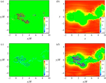
Instantaneous contour maps of the various forcing terms,
 $\mathscr{H}(k_{sgs}-{\it\alpha}(U^{2}/2))f_{{\it\epsilon}}^{T}$
(a),
 $f_{{\it\epsilon}}^{L}$
(b) and
 $\mathscr{H}({\it\alpha}(U^{2}/2)-k_{sgs})f_{{\it\epsilon}}^{W}$
(c), along with the compounded one
 $f_{{\it\epsilon}}$
(d), in the midplane (
 $z/H=0$
). Close-up view in the domain
 $-2<x/H<10$
,
 $-5<y/H<5$
.

The different behaviour of the individual forcing terms in response to different local flow conditions is demonstrated in figure 2, where the three different fields
 $\mathscr{H}(k_{sgs}-{\it\alpha}(U^{2}/2))f_{{\it\epsilon}}^{T}$
,
 $f_{{\it\epsilon}}^{L}$
and
 $\mathscr{H}({\it\alpha}(U^{2}/2)-k_{sgs})f_{{\it\epsilon}}^{W}$
are shown in separate plots, along with the compounded forcing
 $f_{{\it\epsilon}}$
defined by (4.10). The corresponding instantaneous contour maps are drawn at the midplane (
 $z/H=0$
), for the region
 $-2<x/H<10$
,
 $-5<y/H<5$
. The turbulence resolution-based forcing mechanism that is associated with
 $f_{{\it\epsilon}}^{T}$
is apparently working only in the turbulent flow regions. In particular, on the lateral sides of the obstacle, this mechanism becomes active where the transition from laminar to turbulent flow occurs. The force adjusts the wavelet threshold to ensure the desired level of the local ratio of modelled and total dissipations. In the laminar flow regions away from the obstacle, where the forcing term
 $f_{{\it\epsilon}}^{L}$
is dominant, the total force takes positive values, leading to mesh coarsening. In the near-wall and wake regions, the forcing mechanism that is associated with
 $f_{{\it\epsilon}}^{W}$
is non-negligible and negative, which results in local mesh refining. Finally, no forcing scheme is active inside the obstacle, where the threshold field is left to freely diffuse, according to (4.11).
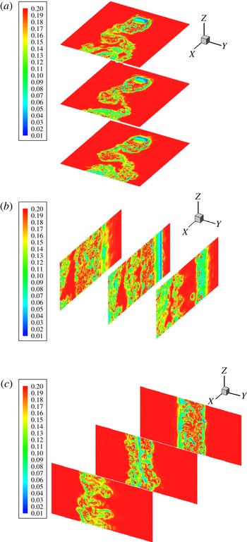
The threshold field that results from the combined action of the above forces is illustrated in figure 3, where the instantaneous contour maps corresponding to the following sets of slices are shown: in the planes
 $z/H=-1.5$
, 0 and 1.5, for the range
 $-2<x/H<7$
and
 $-4<y/H<4$
(a); in the planes
 $y/H=-1$
, 0 and 1, for the range
 $-2<x/H<7$
(b); in the planes
 $x/H=1$
, 2 and 3, for the range
 $-4<y/H<4$
(c). As expected, the threshold variable is relatively high away from the obstacle, where the flow is slightly disturbed and the numerical resolution is maintained to the lowest possible level, which corresponds to
 ${\it\epsilon}=0.2$
. In the turbulent wake behind the body, the threshold variable adapts to the local flow conditions, while tending towards the desired resolution goal. Moreover, in the wall region, the thresholding level tends to diminish. All of this confirms the validity of the compounded forcing scheme adopted in this study.
Instantaneous threshold contours (
 $0.01<{\it\epsilon}<0.2$
) in the planes
 $z/H=-1.5$
, 0 and 1.5, for
 $-2<x/H<7$
,
 $-4<y/H<4$
(a),
 $y/H=-1$
, 0 and 1, for
 $-2<x/H<7$
(b), and
 $x/H=1$
, 2 and 3, for
 $-4<y/H<4$
(c).

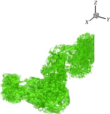
Isosurfaces of
 ${\it\epsilon}=0.12$
at a given time instant. Close-up view in the domain
 $-1<x/H<15$
,
 $-5<y/H<5$
.

Main vortical structures in the cylinder wake identified by the isosurfaces of
 $Q=0.3U^{2}/H^{2}$
(a), and scatter plot of the wavelet collocation points at higher levels of resolution (
 $5\leqslant j\leqslant 8$
) (b), at a given time instant. Close-up view in the domain
 $-1<x/H<15$
,
 $-5<y/H<5$
.

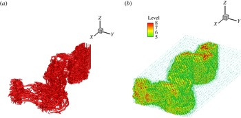
The three-dimensional structure of the threshold field is visualized in figure 4, where the instantaneous isosurfaces of
 ${\it\epsilon}=0.12$
are shown. This figure reflects the wake structure, as can be seen by inspection of figure 5, in panel (a) of which the main vortical structures in the cylinder wake are drawn at the same time instant. Here, the coherent vortices are identified according to the
 $Q$
-criterion, which exploits the second invariant of the velocity-gradient tensor,
 $Q=(|\overline{{\it\Omega}}^{{>}{\it\epsilon}}\!|^{2}-|\overline{\unicode[STIX]{x1D61A}}^{{>}{\it\epsilon}}\!|^{2})/4$
, where
 $|\overline{{\it\Omega}}^{{>}{\it\epsilon}}|=(2\overline{{\it\Omega}}_{ij}^{{>}{\it\epsilon}}\overline{{\it\Omega}}_{ij}^{{>}{\it\epsilon}})^{1/2}$
is the characteristic rate-of-rotation magnitude (Hunt, Wray & Moin Reference Hunt, Wray and Moin1988). This method, which simply defines a vortex as a connected region where
 $Q>0$
, is particularly suitable for examining separated flows. The wake structure is illustrated by reporting the isosurfaces of
 $Q=0.3U^{2}/H^{2}$
. In figure 5(b) the scatter plot of the collocation points associated with the retained wavelets is depicted. For the sake of clarity, the scatter plot, which is coloured by the variable grid level, is reported only for the four highest levels of resolution, namely
 $5\leqslant j\leqslant 8$
. The ability of the present method to dynamically adapt to the flow evolution is apparent as the spatial distribution of active wavelet-collocation points closely resembles that of the main vortical structures. It should be noted, in particular, that the grid points at the highest level of resolution are only present in the regions of large gradients or small-scale flow structures.
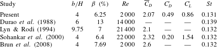
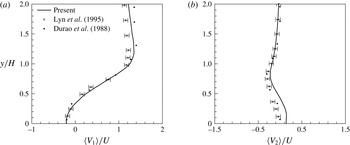
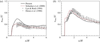
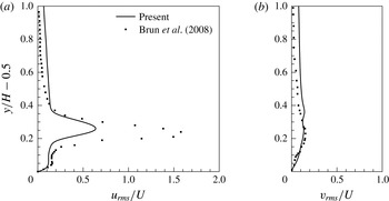
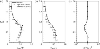
Comparison of the present global results with experimental (Durao, Heitor & Pereira Reference Durao, Heitor and Pereira1988; Lyn & Rodi Reference Lyn and Rodi1994) and computational (Sohankar et al. Reference Sohankar, Davidson and Norberg2000; Brun et al. Reference Brun, Aubrun, Goossens and Ravier2008) reference data.

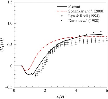
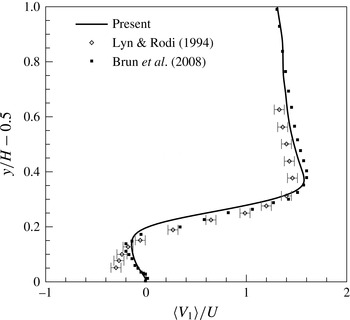
The present results are validated against the experimental data provided by the laser-Doppler velocimetry studies of Durao et al. (Reference Durao, Heitor and Pereira1988), Lyn & Rodi (Reference Lyn and Rodi1994) and Lyn et al. (Reference Lyn, Einav, Rodi and Park1995). Although these works deal with flows at higher Reynolds numbers,
 $Re=14\,000$
and
 $21\,400$
respectively, they are chosen since they represent the standard reference for square cylinder flow simulations. For reference computational data, among the large number of available LES studies, the finite-volume-based studies of Sohankar et al. (Reference Sohankar, Davidson and Norberg2000) and Brun et al. (Reference Brun, Aubrun, Goossens and Ravier2008) are considered. The former study provides a non-adaptive LES solution that uses an energy-based dynamic one-equation model similar to one adopted here, although at
 $Re=22\,000$
, while the latter work provides an LES solution at the present Reynolds number, that is
 $Re=2000$
.
As far as global quantities are concerned, the comparison is summarized in table 1, where the time-averaged drag coefficient
 $\overline{C}_{D}$
, the r.m.s. values of the fluctuations of the drag and lift coefficients, say
 $C_{D}^{\prime }$
and
 $C_{L}^{\prime }$
, and the Strouhal number (
 $St$
) are reported. The mean flow Reynolds number, the aspect ratio
 $b/H$
and the blockage parameter
 ${\it\beta}$
, which characterize the different reference studies, are also indicated in the table. The present results are in good agreement with the experimental and numerical reference data, except for the time-averaged drag coefficient reported in Brun et al. (Reference Brun, Aubrun, Goossens and Ravier2008), which appears to be overestimated.
The resolved velocity field is illustrated by examining the mean streamwise and transverse velocities,
 $\langle V_{1}\rangle$
and
 $\langle V_{2}\rangle$
respectively, which are defined as the time- and spanwise-averaged components of the total velocity vector,
 $V_{i}=U_{i}+\overline{u}_{i}^{{>}{\it\epsilon}}$
, in the
 $(x,y)$
plane. In figure 6, the mean streamwise velocity profile in the near wake (
 $0<x/H<6$
), at the location of the cylinder centreline (
 $y=0$
), is depicted, compared with reference data. In this figure, as well as in the following, the velocity results provided by the experimental works of Lyn and co-authors are reported with the
 $\pm 0.05$
error bands quoted in Lyn et al. (Reference Lyn, Einav, Rodi and Park1995). In figure 7, the mean streamwise velocity profile in the separated boundary layer on the side of the cylinder (
 $0.5<y/H<1.5$
), at the mid location (
 $x=0$
), is drawn. The agreement with reference data is quite good, being almost perfect when referring to the study of Brun et al. (Reference Brun, Aubrun, Goossens and Ravier2008), which is conducted at the same Reynolds number. Furthermore, in figure 8, the mean streamwise and lateral velocity profiles at the location one-half of a side-length downstream of the cylinder,
 $x/H=1$
, in the range
 $0<y/H<2$
, are shown. The comparison with reference experimental data is quite satisfactory. In particular, the extent of the wake is well reproduced, while some slight discrepancies exist in the velocity magnitudes far from the cylinder (
 $y/H>1$
) for the streamwise component (a) and close to the cylinder (
 $y/H<0.5$
) for the lateral one (b). This mismatch is certainly due to the present not fully converged statistics. In the former case, however, the different Reynolds number and blockage ratio that affect the effective oncoming free-stream velocity play a role, as demonstrated by inspection of the reference experimental data.
Longitudinal profile of the mean streamwise velocity in the near wake (
 $0<x/H<6$
), at the location of the cylinder centreline (
 $y=0$
), compared with experimental (Durao et al.
Reference Durao, Heitor and Pereira1988; Lyn & Rodi Reference Lyn and Rodi1994) (diamond and square symbols) and numerical (Sohankar et al.
Reference Sohankar, Davidson and Norberg2000) (dash–dot line) reference data.

Transverse profile of the mean streamwise velocity in the boundary layer on the cylinder side (
 $0.5<y/H<1.5$
), at the mid location (
 $x=0$
), compared with experimental (Lyn & Rodi Reference Lyn and Rodi1994) (diamond symbols) and numerical (Brun et al.
Reference Brun, Aubrun, Goossens and Ravier2008) (square symbols) reference data.

Transverse profiles of the streamwise (a) and lateral (b) mean velocity at the location
 $x/H=1$
in the cylinder wake for
 $0<y/H<2$
, compared with experimental reference data (Lyn et al.
Reference Lyn, Einav, Rodi and Park1995; Durao et al.
Reference Durao, Heitor and Pereira1988) (diamond and square symbols).

Longitudinal profiles of the r.m.s. streamwise (a) and lateral (b) velocity in the near wake (
 $0<x/H<6$
), at the location of the cylinder centreline (
 $y=0$
), compared with experimental (Durao et al.
Reference Durao, Heitor and Pereira1988; Lyn & Rodi Reference Lyn and Rodi1994) (diamond and square symbols) and numerical (Sohankar et al.
Reference Sohankar, Davidson and Norberg2000) (dash–dot line) reference data.

Transverse profiles of the r.m.s. streamwise (a) and lateral (b) velocity on the cylinder side (
 $0.5<y/H<1.5$
), at the mid location (
 $x=0$
), compared with numerical reference data (Brun et al.
Reference Brun, Aubrun, Goossens and Ravier2008) (square symbols).

Transverse profiles of the r.m.s. streamwise (a) and lateral (b) velocity, along with the resolved shear stress (c), at the location
 $x/H=1$
in the cylinder wake for
 $0<y/H<2$
, compared with experimental reference data (Durao et al.
Reference Durao, Heitor and Pereira1988; Lyn et al.
Reference Lyn, Einav, Rodi and Park1995) (diamond and square symbols).

Time histories of the total amounts of resolved (a) and modelled (b) dissipation, for three different prescribed turbulence resolutions (
 $\mathscr{R}_{goal}=0.05$
, 0.10 and 0.15).

In addition, the resolved turbulent stresses are examined. The normal stresses are represented by the r.m.s. variables
 $u_{rms}=\langle u^{\prime }u^{\prime }\rangle ^{1/2}$
and
 $v_{rms}=\langle v^{\prime }v^{\prime }\rangle ^{1/2}$
, where
 $u^{\prime }$
and
 $v^{\prime }$
stand for the streamwise and lateral velocity fluctuations around the associated means respectively. In figure 9, both the r.m.s. profiles in the near wake (
 $0<x/H<6$
), at the location of the cylinder centreline (
 $y=0$
), are depicted, together with the reference experimental and numerical data. The peak of the resolved normal stresses in the transverse direction is located slightly closer to the body and has a slightly greater value than in experiments, which confirms the numerical findings of Sohankar et al. (Reference Sohankar, Davidson and Norberg2000). The r.m.s. profiles in the boundary layer on the side of the cylinder (
 $0.5<y/H<1.5$
), at the mid location (
 $x=0$
), are reported in figure 10. The large discrepancy in the streamwise profiles is mainly due to coarse spanwise resolution used by Brun et al. (Reference Brun, Aubrun, Goossens and Ravier2008). In fact, as stated by the authors, this reference simulation was well-resolved LES in the streamwise and transverse directions, while being close to very-large-eddy simulation (VLES) in the spanwise direction. The comparison with experimental findings is illustrated in figure 11, where the wake transverse r.m.s. profiles are reported at the location
 $x/H=1$
, in the range
 $0<y/H<2$
, along with the reference data (Durao et al.
Reference Durao, Heitor and Pereira1988; Lyn et al.
Reference Lyn, Einav, Rodi and Park1995). In panel (c) of the figure, the profile of the resolved shear stress
 $\langle u^{\prime }v^{\prime }\rangle$
is also considered. Generally, the present results match the reference data rather well, even taking into account the different Reynolds numbers. The existing discrepancies are mostly attributable to the short time window used to collect the velocity statistics, which currently corresponds to approximately four vortex shedding periods.
5.3. Varying resolution
In this work, the wavelet thresholding level varies optimally in both time and space in order to achieve an approximately uniformly accurate computation of the turbulence. The new approach allows the fidelity of the simulation to be varied depending on the prescription of the turbulence resolution parameter
 $\mathscr{R}_{goal}$
, without any change in the underlying numerical method. The key role is thus played by this user-defined coefficient, which directly enters the forcing scheme definition (4.10). To test the robustness and stability of the proposed variable thresholding strategy based on the modelled-to-resolved dissipation ratio (4.3), the following experiment is performed. Once a given turbulence resolution is achieved, the goal value is changed to assess whether and how the solution automatically adjusts to the new level of prescribed resolution. In practice, two different additional calculations are conducted, by decreasing and increasing the initially assigned goal value, which is
 $\mathscr{R}_{goal}=0.10$
, to the new values 0.05 and 0.15 respectively. As expected, for the solution with decreased goal value, the amount of resolved viscous dissipation is augmented and the modelled dissipation is diminished, while the opposite occurs for the solution with increased goal. This is apparent by inspection of figure 12, where the time histories of the total amounts of both dissipations are reported. The lower the goal value is, the higher the resolution and the number of retained wavelets are, as illustrated by the history depicted in figure 13(a). Differently, the amount of resolved kinetic energy appears to be practically the same for the three different solutions, as shown in figure 13(b). This is not surprising because this variable is mostly due to large-scale flow motions, which are however captured, whatever the turbulence resolution of the simulation. In fact, the ratio of modelled to resolved dissipation that is exploited here to control the turbulence resolution is mostly representative of the small-scale flow motions, and the variation in the numerical resolution among the three different solutions mostly occurs at the level of the finest collocation grids. The effectiveness of the present methodology in controlling the turbulence resolution is further demonstrated by considering the backscatter of energy from unresolved to resolved flow motions. In figure 14, the time histories of the total amount of negative SGS dissipation (a) and the percentage of retained wavelet-collocation points where backscatter occurs (b) are reported for the above three different solutions. As expected, by increasing the resolution of the resolved LES field, the importance of the energy backscatter diminishes because flow motions with lower energy are explicitly calculated.
Time histories of the percentage of retained wavelets (a) and total amount of resolved kinetic energy (b), for three different prescribed turbulence resolutions (
 $\mathscr{R}_{goal}=0.05$
, 0.10 and 0.15).

Time histories of the total amount of negative SGS dissipation (a) and associated percentage of retained wavelets (b), for three different prescribed turbulence resolutions (
 $\mathscr{R}_{goal}=0.05$
, 0.10 and 0.15).

Based on this experiment, the effectiveness of the proposed adaptive methodology in controlling the resolution of the simulation is further demonstrated in figure 15, where the scatter plots of the wavelet-collocation points corresponding to the above two solutions with different goals are considered. The figure reports the spatial distribution of active grid points at the midplane (
 $z/H=0$
), in the proximity of the obstacle (
 $-1<x/H<5$
,
 $-3<y/H<3$
), at a given time instant. The scatter plots are coloured by the variable grid level in the range
 $3\leqslant j\leqslant 8$
. The effect of decreasing the goal from
 $\mathscr{R}_{goal}=0.15$
(a) to 0.05 (b), with the subsequent increase of the numerical resolution and the better representation of the dominant flow structures, is apparent. The collocation points in figure 15(a) are practically a subset of those in figure 15(b), which reflects the consistency between different levels of resolution. The present approach thus permits a physics-based automated mesh refinement for capturing regions of locally high flow gradients and small but dynamically important flow structures in an intelligent way.
Scatter plots of the wavelet-collocation points at the midplane (
 $z/H=0$
), at a given time instant, for two different resolution goals, namely
 $\mathscr{R}_{goal}=0.15$
(a) and 0.05 (b). Close-up view in the domain
 $-1<x/H<5$
,
 $-3<y/H<3$
.

6. Concluding remarks
The hybrid volume-penalization/wavelet-collocation method with variable thresholding is developed for the adaptive large-eddy simulation of immersed-body flows. The effectiveness of combining the wavelet-based eddy-capturing approach with the new Lagrangian variable thresholding strategy based on the level of modelled dissipation in simulating bluff-body turbulent flows is demonstrated. The proposed penalized wavelet-based adaptive large-eddy simulation method, supplied with the localized dynamic kinetic-energy-based model, is able to provide high-fidelity solutions for complex flow–structure interaction problems such as those involving three-dimensional flow past bluff bodies. The use of the spatio-temporally varying thresholding strategy allows one to directly control the turbulence resolution/fidelity of the simulations. The results of some numerical experiments for the turbulent flow around a square cylinder at moderately high Reynolds number are in generally good agreement with non-adaptive numerical solutions and experimental findings.
The development of the present fully adaptive methodology represents a fundamental step in the construction of efficient and affordable wavelet-based methods for the numerical simulation of incompressible wall-bounded turbulent flows. Due to the automatic dynamically adaptive meshing, the method completely eliminates the onerous overhead of using grid generation techniques. Thanks to its flexibility and efficiency, the proposed combined method appears to be very promising for the simulation of more challenging flows. For instance, once the less expensive anisotropic wavelet transform is developed, higher-Reynolds-number and/or more complex geometry immersed-body flows will be considered, where the adaptive wavelet-based methods are expected to become even more efficient.
Acknowledgements
This work was supported by the NSF under grant no. CBET-1236505. This support is gratefully acknowledged. The authors are also thankful for the computing time on the Janus supercomputer, which is supported by the National Science Foundation (award no. CNS-0821794) and the University of Colorado Boulder. The Janus supercomputer is a joint effort of the University of Colorado Boulder, the University of Colorado Denver and the National Center for Atmospheric Research.
Appendix A. Wavelet decomposition and WTF
According to definition (2.5), the turbulent velocity field is decomposed using scaling functions
 ${\it\phi}_{\boldsymbol{l}}^{1}$
and wavelet functions
 ${\it\psi}_{\boldsymbol{k}}^{{\it\mu},j}$
with zero mean. The scaling function coefficients
 $c_{\boldsymbol{l}}^{1}$
represent the averaged values of the field, while the wavelet coefficients
 $d_{\boldsymbol{k}}^{{\it\mu},j}$
represent the details of the field at different scales. Due to the local support of both scaling functions and wavelets, there is a one-to-one correspondence between basis function locations and grid points. The coefficients
 $c_{\boldsymbol{l}}^{1}$
and
 $d_{\boldsymbol{k}}^{{\it\mu},j}$
are uniquely associated with a single grid point through the three-dimensional indices
 $\boldsymbol{l}$
and
 $\boldsymbol{k}$
respectively.
In this study, a set of second-generation wavelets known as lifted interpolating wavelets (Sweldens Reference Sweldens1998) is employed. All of the details about the use of the lifted interpolating wavelet transform for constructing efficient wavelet-based numerical methods can be found in Vasilyev & Bowman (Reference Vasilyev and Bowman2000). For example, in the one-dimensional case, the interpolating scaling function and the lifted interpolating wavelet of order
 $3$
are reported, together with their Fourier transforms, in figures 16 and 17 respectively. In fact, first-generation wavelets, which are constructed by discrete dilation and translation of a single mother wavelet, have difficulties in dealing with boundaries, being defined on either infinite or periodic domains. Second-generation wavelets represent a generalization of first-generation ones which supplies the necessary freedom to deal with complex geometries, arbitrary boundary conditions and irregular sampling intervals. As illustrated in figure 17, these wavelets are localized in both physical and wavenumber spaces and have many vanishing polynomial moments. In addition, despite the loss of the translation and the dilation invariance, second-generation wavelets retain many of the useful features of their first-generation counterparts, including a fast transform. The above properties and, in particular, the space/scale localization of the wavelet approach make it an attractive technique for modelling turbulent flows, where the active flow regions to be resolved extend over a broad range of scales, while being not homogeneously distributed in both space and time, which reflects the turbulence intermittency.
One-dimensional interpolating scaling function of order 3, say
 ${\it\phi}={\it\phi}(x)$
(a), and its Fourier transform,
 ${\it\Phi}={\it\Phi}({\it\xi})$
(b).

One-dimensional lifted interpolating wavelet of order 3, say
 ${\it\psi}={\it\psi}(x)$
(a), and its Fourier transform,
 ${\it\Psi}={\it\Psi}({\it\xi})$
(b).

The WTF in wavenumber space for homogeneous turbulence (Goldstein & Vasilyev Reference Goldstein and Vasilyev2004). (a) Energy spectra for the unfiltered (——), filtered (— ⋅ —) and residual (
 $\cdots \cdots$
) velocity fields. (b) Energy spectra associated with the six different wavelet levels (with increasing resolution): level 1 (– – – –), 2 (

 $\cdots \cdots$
), 4 (


As stated in § 2.2, the WTF operator is applied in the wavelet space by means of wavelet coefficient thresholding. This operation can be considered as the explicit application of a nonlinear multi-dimensional spatial filter that depends on each flow realization. To illustrate the spectral properties of the WTF, a couple of figures provided in Goldstein & Vasilyev (Reference Goldstein and Vasilyev2004) are reported here. These figures concern the application of the WTF procedure with six levels of resolution to a
 $256^{3}$
homogeneous isotropic turbulent velocity database, where the grid compression corresponds to retaining 95 % of the available wavelets. In figure 18(a), the energy spectra associated with both the unfiltered and the wavelet-filtered velocity are depicted, along with that corresponding to the residual velocity. It can be seen that, unlike the Fourier cutoff filtered velocity, the wavelet-filtered velocity contains energy all the way down to the smallest resolved scales. In figure 18(b), the energy spectra associated with each level of resolution are shown. It appears that each level has energy in a region of wavenumbers, and these regions significantly overlap.
Appendix B. Localized dynamic procedure
As stated in § 3, the unknown model coefficients for the energy-based closure procedure are determined by exploiting an explicit low-pass test-filtering procedure with width
 $\widehat{{\it\Delta}}$
. Denoting by
 $\widehat{\overline{u}_{i}^{{>}{\it\epsilon}}}$
the test-filtered velocity, the penalized momentum equation, which governs the evolution of the larger resolved turbulent eddies, can be written as
 $$\begin{eqnarray}\frac{\partial \widehat{\overline{u}_{i}^{{>}{\it\epsilon}}}}{\partial t}+(\widehat{\overline{u}_{j}^{{>}{\it\epsilon}}}+U_{j})\frac{\partial \widehat{\overline{u}_{i}^{{>}{\it\epsilon}}}}{\partial x_{j}}=-\frac{\partial \widehat{\overline{P}^{{>}{\it\epsilon}}}}{\partial x_{i}}+{\it\nu}\frac{\partial ^{2}\widehat{\overline{u}_{i}^{{>}{\it\epsilon}}}}{\partial x_{j}\partial x_{j}}-\frac{{\it\chi}_{s}}{{\it\eta}}(\widehat{\overline{u}_{i}^{{>}{\it\epsilon}}}+U_{i})-\frac{\partial \unicode[STIX]{x1D61B}_{ij}}{\partial x_{j}},\end{eqnarray}$$
where
 $\unicode[STIX]{x1D61B}_{ij}=\widehat{\overline{u_{i}u_{j}}^{{>}{\it\epsilon}}}-\widehat{\overline{u}_{i}^{{>}{\it\epsilon}}}\widehat{\overline{u}_{j}^{{>}{\it\epsilon}}}$
stand for the subtest-scale (STS) residual stresses.
The balance equation for the kinetic energy associated with the test-filtered velocity, say
 $k_{rts}=(\widehat{\overline{u}_{i}^{{>}{\it\epsilon}}}\widehat{\overline{u}_{i}^{{>}{\it\epsilon}}})/2$
, is obtained from the previous equation as
 $$\begin{eqnarray}\displaystyle \frac{\partial k_{rts}}{\partial t}+(\widehat{\overline{u}_{j}^{{>}{\it\epsilon}}}+U_{j})\frac{\partial k_{rts}}{\partial x_{j}}\! & = & \displaystyle \!-\widehat{\overline{u}_{i}^{{>}{\it\epsilon}}}\frac{\partial \widehat{\overline{P}^{{>}{\it\epsilon}}}}{\partial x_{i}}+{\it\nu}\frac{\partial ^{2}k_{rts}}{\partial x_{j}\partial x_{j}}-{\it\varepsilon}_{rts}\nonumber\\ \displaystyle & & \displaystyle -\,{\it\Pi}_{sts}-\frac{\partial }{\partial x_{i}}(\widehat{\overline{u}_{j}^{{>}{\it\epsilon}}}\unicode[STIX]{x1D61B}_{ij})-\frac{{\it\chi}_{s}}{{\it\eta}}(2k_{rts}+\widehat{\overline{u}_{i}^{{>}{\it\epsilon}}}U_{i}),\end{eqnarray}$$
where
 ${\it\Pi}_{sts}=-\unicode[STIX]{x1D61B}_{ij}(\partial \widehat{\overline{u}_{i}^{{>}{\it\epsilon}}}/\partial x_{j})\equiv -\unicode[STIX]{x1D61B}_{ij}\widehat{\overline{\unicode[STIX]{x1D61A}}_{ij}^{{>}{\it\epsilon}}}$
represents the STS dissipation, that is, the rate at which energy is locally transferred from resolved to unresolved motions at the test level, while
 ${\it\varepsilon}_{rts}={\it\nu}((\partial \widehat{\overline{u}_{i}^{{>}{\it\epsilon}}}/\partial x_{j})(\partial \widehat{\overline{u}_{i}^{{>}{\it\epsilon}}}/\partial x_{j}))$
is the corresponding pseudo-dissipation.
The STS turbulent kinetic energy is defined as the analogue of the SGS energy but at the test-filter level, namely as the difference between the test-filtered kinetic energy and the kinetic energy of the test-filtered velocity field, that is,
 $$\begin{eqnarray}k_{sts}={\textstyle \frac{1}{2}}\widehat{\overline{u_{i}u_{i}}^{{>}{\it\epsilon}}}-{\textstyle \frac{1}{2}}\widehat{\overline{u}_{i}^{{>}{\it\epsilon}}}\widehat{\overline{u}_{i}^{{>}{\it\epsilon}}}=\widehat{\overline{k}^{{>}{\it\epsilon}}}-k_{rts},\end{eqnarray}$$
or, equivalently,
 $k_{sts}=\unicode[STIX]{x1D61B}_{ii}/2$
. The evolution equation for this variable is derived by test-filtering equation (3.4) and combining with (B 2):
 $$\begin{eqnarray}\displaystyle \frac{\partial k_{sts}}{\partial t}+(\widehat{\overline{u}_{j}^{{>}{\it\epsilon}}}+U_{j})\frac{\partial k_{sts}}{\partial x_{j}}\! & = & \displaystyle \!{\it\nu}\frac{\partial ^{2}k_{sts}}{\partial x_{j}\partial x_{j}}-\frac{\partial }{\partial x_{i}}(\widehat{\overline{u_{i}P}^{{>}{\it\epsilon}}}-\widehat{\overline{u}_{i}^{{>}{\it\epsilon}}}~\widehat{\overline{P}^{{>}{\it\epsilon}}})-{\it\varepsilon}_{sts}\nonumber\\ \displaystyle & & \displaystyle +\,{\it\Pi}_{sts}+\frac{\partial }{\partial x_{i}}(\widehat{\overline{u}_{j}^{{>}{\it\epsilon}}}\unicode[STIX]{x1D61B}_{ij})-\frac{{\it\chi}_{s}}{{\it\eta}}(2k_{sts}),\end{eqnarray}$$
where
 ${\it\varepsilon}_{sts}$
stands for the STS energy dissipation,
 $$\begin{eqnarray}{\it\varepsilon}_{sts}={\it\nu}\left(\widehat{\overline{\frac{\partial u_{i}}{\partial x_{j}}\frac{\partial u_{i}}{\partial x_{j}}}^{{>}{\it\epsilon}}}-\frac{\partial \widehat{\overline{u}_{i}^{{>}{\it\epsilon}}}}{\partial x_{j}}\frac{\partial \widehat{\overline{u}_{i}^{{>}{\it\epsilon}}}}{\partial x_{j}}\right)=\widehat{\overline{{\it\varepsilon}}^{{>}{\it\epsilon}}}-{\it\varepsilon}_{rts}.\end{eqnarray}$$
In practice, by analogy with (3.10), the transport model equation for the STS energy can be rewritten as
 $$\begin{eqnarray}\frac{\partial k_{sts}}{\partial t}+(\widehat{\overline{u}_{j}^{{>}{\it\epsilon}}}+U_{j})\frac{\partial k_{sts}}{\partial x_{j}}=\frac{\partial }{\partial x_{j}}\left[({\it\nu}+{\it\nu}_{t})\frac{\partial k_{sts}}{\partial x_{j}}\right]-{\it\varepsilon}_{sts}+{\it\Pi}_{sts}-\frac{{\it\chi}_{s}}{{\it\eta}}(2k_{sts}).\end{eqnarray}$$
Here, similarly to the SGS stresses and SGS energy dissipation, the STS stresses and STS energy dissipation are approximated by
 $$\begin{eqnarray}\unicode[STIX]{x1D61B}_{ij}\cong {\textstyle \frac{2}{3}}k_{sts}{\it\delta}_{ij}-2C_{{\it\nu}}\widehat{{\it\Delta}}k_{sts}^{1/2}\widehat{\overline{\unicode[STIX]{x1D61A}_{ij}}^{{>}{\it\epsilon}}}\end{eqnarray}$$
and
 $$\begin{eqnarray}{\it\varepsilon}_{sts}\cong C_{{\it\varepsilon}}k_{sts}^{3/2}/\widehat{{\it\Delta}}\end{eqnarray}$$
respectively, while employing the same model coefficients
 $C_{{\it\nu}}$
and
 $C_{{\it\varepsilon}}$
as used in (3.3) and (3.9), due to the scale-invariance assumption.
The model coefficient
 $C_{{\it\nu}}$
for the turbulent eddy viscosity (3.2) is determined by exploiting the following Germano-like identities for the deviatoric and hydrostatic stresses:
 $$\begin{eqnarray}\unicode[STIX]{x1D61B}_{ij}^{\ast }-\widehat{{\it\tau}_{ij}^{\ast }}=\unicode[STIX]{x1D613}_{ij}^{\ast }\end{eqnarray}$$
and
 $$\begin{eqnarray}k_{sts}-\widehat{k_{sgs}}=k_{L}\end{eqnarray}$$
respectively, where
 $\unicode[STIX]{x1D613}_{ij}=\widehat{\overline{u_{i}}^{{>}{\it\epsilon}}\overline{u_{j}}^{{>}{\it\epsilon}}}-\widehat{\overline{u}_{i}^{{>}{\it\epsilon}}}\widehat{\overline{u}_{j}^{{>}{\it\epsilon}}}$
are the known Leonard stresses and
 $k_{L}=\unicode[STIX]{x1D613}_{ii}/2$
. Combining these equations with the modelling approximations (3.3) and (B 7), a classical least-squares solution (Lilly Reference Lilly1992) provides the following equation in the only unknown variable
 $C_{{\it\nu}}(\boldsymbol{x},t)$
:
 $$\begin{eqnarray}C_{{\it\nu}}\widehat{{\it\Delta}}=\frac{\unicode[STIX]{x1D613}_{ij}^{\ast }\unicode[STIX]{x1D614}_{ij}}{\unicode[STIX]{x1D614}_{pq}\unicode[STIX]{x1D614}_{pq}},\end{eqnarray}$$
because the quantity
 $$\begin{eqnarray}\unicode[STIX]{x1D614}_{ij}=\widehat{k_{sgs}^{1/2}\overline{\unicode[STIX]{x1D61A}_{ij}}^{{>}{\it\epsilon}}}-2(\widehat{k_{sgs}}+k_{L})^{1/2}\widehat{\overline{\unicode[STIX]{x1D61A}_{ij}}^{{>}{\it\epsilon}}}\end{eqnarray}$$
is directly computable from the resolved velocity and SGS energy fields.
As regards the second model parameter to be determined,
 $C_{{\it\varepsilon}}$
, another Germano-like identity can be written for the energy dissipation rates according to
 $$\begin{eqnarray}{\it\varepsilon}_{sts}-\widehat{{\it\varepsilon}_{sgs}}={\it\varepsilon}_{L},\end{eqnarray}$$
where the Leonard-like term
 $$\begin{eqnarray}{\it\varepsilon}_{L}={\it\nu}\left(\widehat{\frac{\partial \overline{u}_{i}^{{>}{\it\epsilon}}}{\partial x_{j}}\frac{\partial \overline{u}_{i}^{{>}{\it\epsilon}}}{\partial x_{j}}}-\frac{\partial \widehat{\overline{u}_{i}^{{>}{\it\epsilon}}}}{\partial x_{j}}\frac{\partial \widehat{\overline{u}_{i}^{{>}{\it\epsilon}}}}{\partial x_{j}}\right)\end{eqnarray}$$
is known. Here, following Menon & Kim (Reference Menon and Kim1996), the above definition is slightly modified as
 $$\begin{eqnarray}{\it\varepsilon}_{L}=({\it\nu}+{\it\nu}_{t})\left(\widehat{\frac{\partial \overline{u}_{i}^{{>}{\it\epsilon}}}{\partial x_{j}}\frac{\partial \overline{u}_{i}^{{>}{\it\epsilon}}}{\partial x_{j}}}-\frac{\partial \widehat{\overline{u}_{i}^{{>}{\it\epsilon}}}}{\partial x_{j}}\frac{\partial \widehat{\overline{u}_{i}^{{>}{\it\epsilon}}}}{\partial x_{j}}\right),\end{eqnarray}$$
due to the fact that the energy
 $k_{L}$
is actually dissipated also due to turbulent eddy viscosity.
Finally, combining (B 13) with the approximations (3.9) and (B 8), while employing (B 10), the following equation in the only unknown variable
 $C_{{\it\varepsilon}}(\boldsymbol{x},t)$
is obtained:
 $$\begin{eqnarray}\frac{C_{{\it\varepsilon}}(\widehat{k_{sgs}}+k_{L})^{3/2}}{\widehat{{\it\Delta}}}-\frac{C_{{\it\varepsilon}}\widehat{k_{sgs}^{3/2}}}{{\it\Delta}}={\it\varepsilon}_{L}.\end{eqnarray}$$
It is worth noting that both the resolving equations (B 11) and (B 16) are based on the assumption that the model coefficients
 $C_{{\it\nu}}$
and
 $C_{{\it\varepsilon}}$
vary slowly in space so that they can be taken out of the test-filtering operation. In this study, the absence of abrupt jumps in the values of these coefficients is also guaranteed by the use of the adjacent zone in the wavelet grid adaptation process.