2.1. Computation details

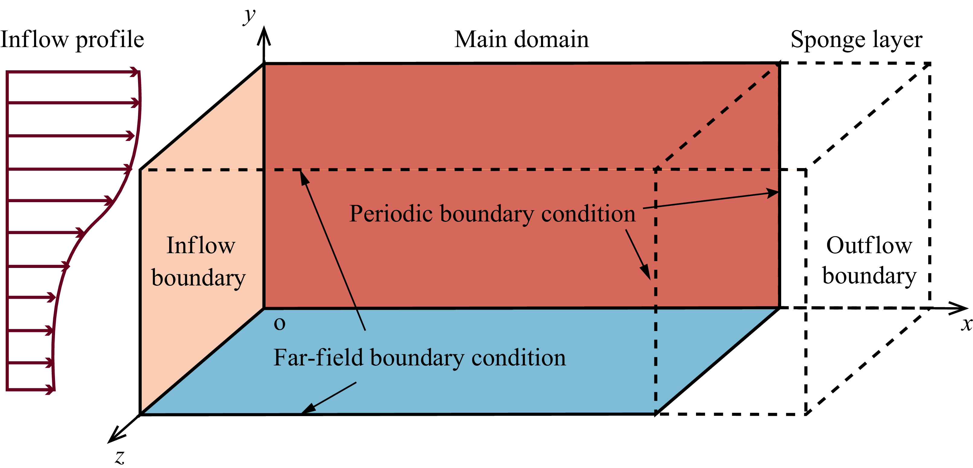
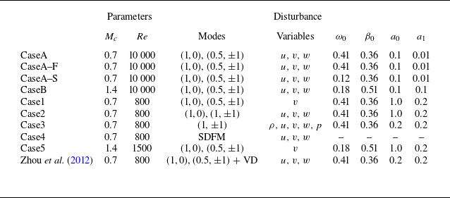
A spatially developing compressible mixing layer is studied through DNS. The configuration of the mixing layer is illustrated in figure 1. Nine simulation cases are considered, with different parameters and types of disturbance, as detailed in table 1. The mixing layer, initially in a laminar state, is characterised by a thin layer between two free streams with distinct streamwise velocities but uniform density and pressure. In this study, the laminar properties of the mixing layer are employed to define a non-dimensionalised system. Laminar density, streamwise velocity, temperature and viscosity for the upper high-speed and lower low-speed streams are denoted as $\rho ^*_1$ , $U^*_1$ , $T^*_1$ , $\mu _1^*$ and $\rho ^*_2$ , $U^*_2$ , $T^*_2$ , $\mu ^*_2$ , respectively. The quantities of the upper stream, e.g. $\rho ^*_1$ , serve as reference scalings. The length scale is defined as $\delta _\omega ^*=\Delta U^*/|\mathrm d\bar {u}^*/\mathrm d y|_{max}$ , referred to as the ‘vorticity thickness’ of the mixing layer, where $\Delta U^*$ represents the velocity difference between the high- and low-speed layers, while $\mathrm{d}\bar {u}^*/\mathrm{d}y$ denotes the derivative of initial streamwise velocity in the normal direction. Consequently, the Reynolds number and Mach number are defined as $Re =\rho ^*_1U^*_1\delta ^*_{\omega }/\mu ^*_1$ and $Ma=U^*_1/\sqrt {\gamma RT^*_1}$ , where $\gamma = 1.4$ represents the heat capacity ratio, and $R = 8.314$ J K⁻¹ mol⁻¹ is the universal gas constant.

Figure 1.

Schematic of the computational domain, boundary conditions and basic laminar flow.

Table 1.

Numerical settings for present simulations. The disturbance is in the form $u_i^{\prime}=\text{Re}[a_0\, \phi _0(y)\,e^{-i\omega _0} + a_1\,\phi _1^+(y)\,\textrm{e}^{\textrm{i}(\beta _0z-\omega _1t)} + a_1\,\phi _1^-(y)\,\textrm{e}^{\textrm{i}(-\beta _0z-\omega _1t)}]$ . A normalised notation $(\omega /\omega _0, \beta /\beta _0)$ is used for mode description. The first digit indicates multiples of the fundamental streamwise frequency $\omega _0$ , and the second digit refers to multiples of the fundamental spanwise wavenumber $\beta _0$ . Here, ‘SDFM’ means the synthetic digital filtering method (Klein, Sadiki & Janicka Reference Klein, Sadiki and Janicka2003), and ‘VD’ denotes vortical disturbance.

In this study, we continue to use the computational domain specified by Zhou et al. (Reference Zhou, He and Shen2012), which is defined as $[0, 54L_x]\times [-L_y/2, L_y/2]\times [0,2L_z]$ , where $L_x=2\unicode{x03C0} /\alpha$ , $L_y=400$ and $L_z=2\unicode{x03C0} /\beta$ , with $\alpha =0.54$ and $\beta =0.36$ representing the most unstable wavenumbers from linear stability theory (LST). The domain is bounded by inflow and outflow boundaries in the streamwise ( $x$ ) direction, two non-reflecting boundaries in the normal ( $y$ ) direction, and two periodic boundaries in the spanwise ( $z$ ) direction. The dimensionless velocities of upper stream $U_1$ and lower stream $U_2$ are set to 1.0 and 0.5, respectively. The Reynolds number and the reference Mach number are specified as 800 and 2.8, respectively, for low-Mach cases (Case1–Case4). Those two parameters are 1500 and 5.6, respectively, for the high-Mach case (Case5). For CaseA and CaseB, the Reynolds number is set to 10 000 to validate the growth rate of unstable waves by by comparing it with the corresponding mode amplification rates calculated from LST. Assuming equal specific heats and temperatures yields a convective Mach number $M_c = (Ma_1 - Ma_2)/2=0.7$ or $1.4$ . The pressures of both free streams are identical to each other and equal to $1/(\gamma\, Ma_1^2)$ . At the inflow boundary, the unperturbed basic inflow profile of the streamwise velocity is obtained by solving compressible boundary layer equations. In addition, the inflow is forced by 3-D unstable waves. Readers are encouraged to consult Appendix A for more detailed description of how the disturbances are imposed.

The non-dimensionalised compressible Navier–Stokes equations are solved numerically using a finite difference solver on non-staggered grids, which read

(2.1) \begin{align}\frac {\partial \rho }{\partial t}+\boldsymbol{\nabla }\boldsymbol{\cdot }(\rho \boldsymbol{u})=0,\end{align}

(2.2) \begin{align}\frac {\partial \rho \boldsymbol{u}}{\partial t} + \boldsymbol{\nabla }\boldsymbol{\cdot }(\rho \boldsymbol{u} \boldsymbol{u} - \boldsymbol{\tau }) = 0,\end{align}

(2.3) \begin{align}\frac {\partial \rho E}{\partial t} + \boldsymbol{\nabla }\boldsymbol{\cdot }(\rho E \boldsymbol{u} - \boldsymbol{\tau } \boldsymbol{u}) = \boldsymbol{q}.\end{align}

Here, $\rho$ , $\boldsymbol{u}=(u,v,w)$ and $E=C_VT+1/2|\boldsymbol{u}|^2$ represent the fluid density, velocity and total energy per unit mass, respectively. The specific heat capacity at constant volume $C_V$ is expressed as $1/\gamma (\gamma -1)\,Ma^2_1$ . The shear stress tensor and heat flux are denoted by $\boldsymbol{\tau }=\tau _{ij}$ and $\boldsymbol{q}=q_i$ , respectively, and take the forms

(2.4) \begin{align} \tau _{ij} = -p\,\delta _{ij} + \frac {2\mu }{Re }\left(S_{ij}-\frac {1}{3}\boldsymbol{\nabla }\boldsymbol{\cdot }\boldsymbol{u}\,\delta _{ij}\right) \end{align}

and

(2.5) \begin{align} q_i=-\frac {\mu }{(\gamma -1)\,Ma_1^2\,Re\,Pr}\frac {\partial T}{\partial x_i}. \end{align}

Here, $p$ is pressure, $T$ is temperature, and $ \unicode{x1D64E} = S_{ij} = 1/2 (\partial u_i /\partial x_j+\partial u_j /\partial x_i)$ is the strain rate tensor. The dynamic viscosity $\mu$ is evaluated using Sutherland’s law, and $Pr = 0.7$ denotes the Prandtl number. The above equations are complemented by the perfect gas law $p=\rho T/\gamma Ma_1^2$ .

The nonlinear terms in (2.2) are discretised using a hybrid seventh-order linear scheme, a seventh-order weighted essentially non-oscillatory (WENO) scheme, and a fifth-order WENO scheme (Shu Reference Shu1998). The viscous terms are discretised using an eighth-order-accurate central difference scheme. Temporal advancement of the equations is achieved using a third-order total variation diminishing Runge–Kutta multistage method. In Case1, for example, the grid numbers are $4160$ , $350$ and $256$ along the $x$ -, $y$ - and $z$ -directions, respectively. In the $x$ -direction, the first 4000 grid points are uniformly spaced from $x= 0$ to $x=50L_x$ , while the remaining 160 grid points are stretched from $x=50L_x$ to $x = 54L_x$ to create a buffer range. In the normal direction, to capture fine structures in the mixing layer, the grid is concentrated in the middle zone and stretched to the far-field boundaries. Approximately 46 grid points are distributed within the early-stage centre layer around the inflow region, which remains predominantly laminar, while approximately 115 grid points are allocated within the downstream centre layer close to the outflow region, which reaches the fully turbulent state (the corresponding results are not shown here). The numerical settings are validated by comparing the averaged streamwise velocity profile in the fully developed turbulent region with that reported by Zhou et al. (Reference Zhou, He and Shen2012), as shown in figure 2. The computations are accelerated by Nvidia V100 GPU cards.

Figure 2.

Profiles of the mean streamwise velocity $\bar u$ across mixing layers within the fully developed turbulent region for different cases. The numerical data from Zhou et al. (Reference Zhou, He and Shen2012) are included for comparison.

2.2. Linear stability analysis

It is essential to validate whether the numerical code is efficient for flows involving both shockwaves and growth of instabilities (Sandham & Yee Reference Sandham and Yee1989). To this end, the value of the imaginary part of the most unstable streamwise wavenumber $\alpha _{0,i}$ needs to be compared with the growth rate of mode energy calculated by DNS as suggested by Kim, Moin & Moser (Reference Kim, Moin and Moser1987). The detailed derivation of LST equations follows Sandham (Reference Sandham1989). One can start with the Eulerian equations in the form

(2.6a) \begin{gather} \frac {\partial \rho }{\partial t}+u_i \frac {\partial \rho }{\partial x_i}+\rho \frac {\partial u_i}{\partial x_i}=0, \end{gather}

(2.6b) \begin{gather} \rho \left (\frac {\partial u_i}{\partial t}+u_j \frac {\partial u_i}{\partial x_j}\right )=-\frac {1}{\gamma M_1^2} \frac {\partial p}{\partial x_i}, \end{gather}

(2.6c) \begin{gather} \rho \left (\frac {\partial T}{\partial t}+u_i \frac {\partial T}{\partial x_i}\right )=-p(\gamma -1) \frac {\partial u_i}{\partial x_i}, \end{gather}

(2.6d) \begin{gather} p=\rho T. \end{gather}

Decomposing the flow variables into a basic flow part and a disturbance part, and assuming travelling wave solutions for the latter, i.e.

(2.7) \begin{align}u=\bar {u}+u^{\prime }, \quad v=v^{\prime },\quad w=w^{\prime },\quad T=\bar {T}+T^{\prime },\quad \rho =\bar {\rho }+\rho ^{\prime },\quad p=1+p^{\prime },\end{align}

(2.8) \begin{align}\left (u^{\prime }, v^{\prime }, w^{\prime }, T^{\prime }, \rho ^{\prime }, p^{\prime }\right )=(\hat {u}, \hat {v}, \hat {w}, \hat {T}, \hat {\rho }, \hat {p})\, \textrm{e}^{\textrm{i}(\alpha x+\beta z-\omega t)},\end{align}

one can readily obtain the linearised disturbance equations

(2.9a) \begin{gather} \hat {\rho } i(\alpha \bar {u}-\omega )+\hat {v}\, \textrm{D} \bar {\rho }+\bar {\rho }[i(\alpha \hat {u}+\beta \hat {w})+\textrm{D} \hat {v}]=0, \end{gather}

(2.9b) \begin{gather} \bar {\rho }[i(\alpha \bar {u}-\omega ) \hat {u}+\hat {v}\, \textrm{D} \bar {u}]=\frac {-i \alpha \hat {p}}{\gamma M_1^2}, \end{gather}

(2.9c) \begin{gather} \bar {\rho } i(\alpha \bar {u}-\omega ) \hat {v}=\frac {-\textrm{D} \hat {p}}{\gamma M_1^2}, \end{gather}

(2.9d) \begin{gather} \bar {\rho } i(\alpha \bar {u}-\omega ) \hat {w}=\frac {-i \beta \hat {p}}{\gamma M_1^2}, \end{gather}

(2.9e) \begin{gather} \bar {\rho }[i(\alpha \bar {u}-\omega ) \hat {T}+\hat {v}\, \textrm{D} \bar {T}]=-(\gamma -1)[i(\alpha \hat {u}+\beta \hat {w})+\textrm{D} \hat {v}], \end{gather}

(2.9f) \begin{gather} \hat {p}=\bar {\rho } \hat {T}+\hat {\rho } \bar {T}, \end{gather}

with $\textrm{D}\equiv \mathrm{d}/\mathrm{d}y$ denoting the derivative operator with respect to $y$ . For a spatially developing mixing layer, the disturbance equations can be written as a linear system $A_s \boldsymbol x = \alpha B_s \boldsymbol x$ , where $\boldsymbol x=(\hat \rho ,\hat u,\hat v,\hat w,\hat T)^{\rm T}$ :

(2.10) \begin{align} A_s=\left (\begin{array}{ccccc} \omega & 0 & i(\textrm{D} \bar {\rho }+\bar {\rho }\, \textrm{D}) & -\beta \bar {\rho } & 0 \\[3pt] 0 & \omega & i\, \textrm{D} \bar {u} & 0 & 0 \\[3pt] \frac {i(\textrm{D} \bar {T}+\bar {T}\, \textrm{D})}{\bar {\rho } \gamma M_1^2} & 0 & \omega & 0 & \frac {i(\textrm{D} \bar {\rho }+\bar {\rho }\, \textrm{D})}{\bar {\rho } \gamma M_1^2} \\[3pt] \frac {-i \beta \bar {T}}{\bar {\rho } \gamma M_1^2} & 0 & 0 & \omega & \frac {-\beta }{\gamma M_1^2} \\[3pt] 0 & 0 & i\left (\textrm{D} \bar {T}+\frac {(\gamma -1)\, \textrm{D}}{\bar {\rho }}\right ) & \frac {-(\gamma -1) \beta }{\bar {\rho }} & \omega \end{array}\right ) \end{align}

and

(2.11) \begin{align} B_s=\left (\begin{array}{ccccc} \bar {u} & \bar {\rho } & 0 & 0 & 0 \\ \frac {T}{\bar {\rho }} & \bar {u} & 0 & 0 & \frac {1}{\gamma M_1^2} \\ \bar {\rho } M_1^2 & 0 & \bar {u} & 0 & 0 \\ 0 & 0 & 0 & \bar {u} & 0 \\ 0 & \frac {\gamma -1}{\bar {\rho }} & 0 & 0 & \bar {u} \end{array}\right ). \end{align}

The second-order central difference scheme is employed to discretise the differential operators in matrix $A_s$ of the disturbance equation system. Shown in figure 3(a,b) are the spatial amplification rate of the mixing layer ( $-\alpha _i$ ) against frequency $\omega$ at $Mc=0.01$ , and that against the angle of oblique waves $\theta$ for different convective Mach numbers and frequencies, respectively, which are calculated through linear instability analysis. The correctness of present results and reliability of our code are validated in comparison with the corresponding results from Sandham (Reference Sandham1989), who used the shooting method to solve the eigenvalue problem. Note that it is within expectation that the direct method loses some accuracy near the neutral mode. It is hard to capture weak amplified waves, especially at high Mach numbers. However, the direct method is faster than the shooting method, and meets the accuracy requirement near the most unstable mode. 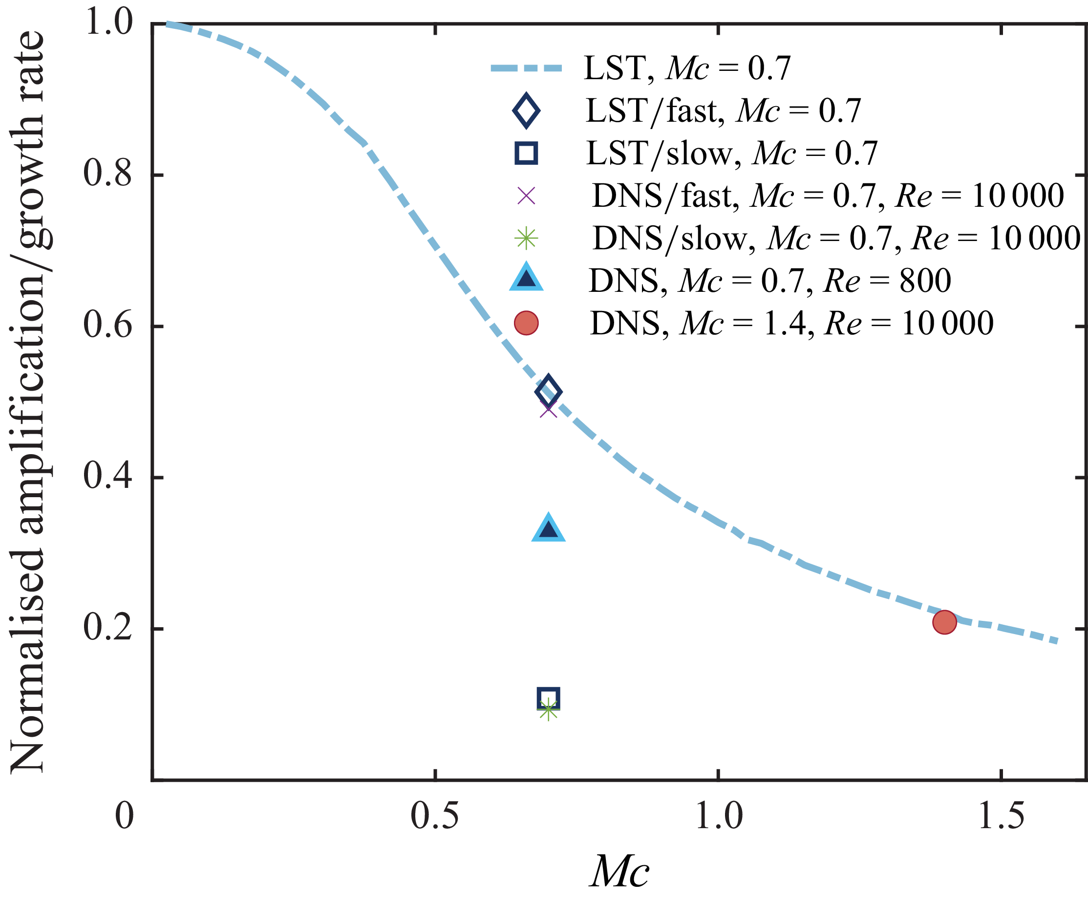Furthermore, figure 4 provides a comparison between the imaginary part of the most unstable wavenumber $-\alpha _{0,i}$ from LST and (half) the growth rate of mode kinetic energy $E_k(\omega ,\beta )=\int _{-L_y/2}^{L_y/2}\hat u_i \hat u_i^c\,\mathrm{d}y$ from DNS for two convective Mach numbers (0.7 and 1.4), which validates the effectiveness of the present numerical code.

Figure 3.

(a) Spatial amplification rate of the mixing layer ( $-\alpha _i$ ) against frequency $\omega$ at $Mc=0.01$ . (b) Spatial amplification rate of the mixing layer ( $-\alpha _i$ ) against the angle of oblique waves $\theta$ for different convective Mach numbers and frequencies, which are calculated through linear stability analysis. In (b), the black lines denote present results, while solid coloured lines represent the calculations from Sandham (Reference Sandham1989).

To further validate the effectiveness of the present numerical code in capturing the subsonic and supersonic modes, both the LST and DNS results are obtained for the subsonic (fast) and supersonic (slow) modes of the test case with $Mc=0.7$ . Those two numerical simulations correspond to CaseA–F and CaseA–S as listed in table 1. The amplification rates of fast and slow modes given by LST are $-\alpha _i= 0.063$ and 0.013, respectively. As expected, the most amplified mode is the fast mode, in good consistency with the conclusion from either Sandham (Reference Sandham1989) or Grosch & Jackson (Reference Grosch and Jackson1991). The corresponding amplification rates from DNS are also presented in figure 4, which turn out to be in good alignment with LST. These calculations confirm the validity of the employed code in capturing the subsonic and supersonic modes.

Figure 4.

The spatial amplification rate of the most unstable wave ( $\alpha _{0,i}$ ) from LST (dashed line) and half the growth rate of kinetic energy $E_k(\omega /\omega _0,\beta /\beta _0)$ in mode $(1,0)$ from DNS against the convective Mach number ( $Mc$ ). The results of both subsonic (fast) and supersonic (slow) modes from LST and DNS are also provided for comparison in the test case $Mc=0.7$ . The amplification rate and growth rate are normalised by their incompressible counterparts, respectively.

2.3. Measurement of deformation

Building upon the data generated by DNS, a theoretical analysis is conducted to quantitatively investigate the mechanism of wave–vortex interaction. This analysis is rooted in the governing equation of vorticity ( $\boldsymbol{\omega }=\boldsymbol{\nabla }\boldsymbol{\cdot} \boldsymbol{u}$ )

(2.12) \begin{align} \begin{aligned} \frac {\partial \boldsymbol{\omega }}{\partial t} = & - (\boldsymbol{u} \boldsymbol{\cdot }\boldsymbol{\nabla }) \boldsymbol{\omega } - \boldsymbol{\omega }(\boldsymbol{\nabla }\boldsymbol{\cdot }\boldsymbol{u}) + (\boldsymbol{\omega } \boldsymbol{\cdot }\boldsymbol{\nabla }) \boldsymbol{u}-\frac {1}{\rho ^2} \boldsymbol{\nabla }p \boldsymbol{\cdot} \boldsymbol{\nabla }\rho \\ & +\frac {\mu }{ {Re }}\left [\frac {1}{\rho } {\nabla} ^2 \boldsymbol{\omega }-\frac {1}{\rho ^2} \boldsymbol{\nabla }\rho \boldsymbol{\cdot} \left ({\nabla} ^2 \boldsymbol{u}+\frac {1}{3} \boldsymbol{\nabla }(\boldsymbol{\nabla }\boldsymbol{\cdot }\boldsymbol{u})\right )\right ]. \end{aligned} \end{align}

The terms on the right-hand side of (2.12) represent the contributions of convection, dilation, stretching/tilting, baroclinic effect and viscous dissipation, respectively. Vortex stretching and tilting lead to the creation of $\Lambda$ -shaped and subsequent hairpin vortices. The production of enstrophy ( $\boldsymbol{\omega }^2/2$ , which measures the vortex intensity) by vortex stretch/tilting can be expressed as

(2.13) \begin{align} \boldsymbol{\omega } \boldsymbol{\cdot }\boldsymbol{\nabla }\boldsymbol{u} \boldsymbol{\cdot }\boldsymbol{\omega } = \boldsymbol{\omega }^\textrm{T} \unicode{x1D64E} \boldsymbol{\omega }, \end{align}

where $ \unicode{x1D64E}=(1/2)[\boldsymbol{\nabla }\boldsymbol{u} + (\boldsymbol{\nabla }\boldsymbol{u})^\textrm{T}]$ is the strain rate tensor. To describe the geometry, orientation and dynamics of vortices, the analyis is usually carried out based on the eigenvalues and eigenvectors of strain rate tensor $ \unicode{x1D64E}$ , as reported by Kida & Tanaka (Reference Kida and Tanaka1994) for homogeneous shear flows, and Bechlars & Sandberg (Reference Bechlars and Sandberg2017) for boundary layer flows. For example, the production term (2.13) can be further decomposed into

(2.14) \begin{align} \boldsymbol{\omega }^\textrm{T} \unicode{x1D64E}\boldsymbol{\omega } = 2|\unicode{x1D63C}|^2|\unicode{x1D64E}|\sum ^3_{i=1}\beta _i\cos ^2(\left \langle \boldsymbol{\omega },\boldsymbol{\varLambda }_i\right \rangle ), \end{align}

where $ \unicode{x1D63C}=(1/2)[\boldsymbol{\nabla }\boldsymbol{u} - (\boldsymbol{\nabla }\boldsymbol{u})^\textrm{T}]$ is the asymmetric part of the velocity gradient, and $\beta _i$ ( $i=1,2,3$ ) and $\boldsymbol{\varLambda }_i$ are the normalised eigenvalues and eigenvectors of the strain rate tensor, respectively. The angles between vorticity vector and eigenvectors are denoted by $\langle \boldsymbol{\omega },\boldsymbol{\varLambda }_i\rangle$ .

For the Lagrangian description of coherent structures, a set of timelines or the time sequence of a material surface can be used to visualise the evolving history of a parcel of fluids. To this end, a line or plane of particle tracers is released at a specific instant and position of the flow field, then tracked in time based on the Lagrangian method (Jiang et al. Reference Jiang, Gu, Lee, Smith and Linden2021). Given a velocity field $\boldsymbol{u}(\boldsymbol{x},t)$ , the path of each particle $\boldsymbol{X}(t)$ can be obtained by integrating the ordinary differential equation

(2.15) \begin{align} \dot {\boldsymbol{X}} = \boldsymbol{u}(\boldsymbol{X},t), \quad t \in [t_0,t_1], \end{align}

with solution $\boldsymbol{X}(t;t_0,\boldsymbol{X}_0)$ . Thus the Lagrangian description of fluid motion takes the form of a flow map $F_{t_0}^t$ :

(2.16) \begin{align} F_{t_0}^t(\boldsymbol{X}_0) = \boldsymbol{X}(t;t_0,\boldsymbol{X}_0), \quad t \in [t_0,t_1]. \end{align}

As far as a hypersurface in a 3-D space is concerned, an evolving material line $\boldsymbol{L}$ or a material surfaces $\boldsymbol{M}$ initiated at time $t_0$ can be defined as

(2.17) \begin{align} \boldsymbol{L}(t) := F^t_{t_0}(\boldsymbol{L}(t_0)) \end{align}

and

(2.18) \begin{align} \boldsymbol{M}(t) := F^t_{t_0}(\boldsymbol{M}(t_0)), \end{align}

respectively. In this study, the timelines and material surfaces are released at positions within the mixing layer. The metamorphosis of the material elements can reveal the evolution of flow structures, a process that is challenging to discern within the Eulerian framework.

To quantitatively investigate the relationship between the deformation of material elements (lines or surfaces) and flow structures, we calculate the geometric characteristics of material entities. In continuum mechanics, the deformation of an object is typically represented by strain tensors, such as the Cauchy–Green tensor

(2.19) \begin{align} C(\boldsymbol{X}_0) = [\boldsymbol{\nabla }F^t_{t_0}(\boldsymbol{X}_0)]^\textrm{T}\, \boldsymbol{\nabla }F^t_{t_0}(\boldsymbol{X}_0). \end{align}

The stretching of fluids in the Lagrangian framework can be determined through considering the eigencharacter of the Cauchy–Green tensor, such as the finite-time Lyapunov exponent (FTLE) and the alignment of eigenvectors. Specifically, the FTLE is introduced below for the purpose of visualising fluid stretching (Haller Reference Haller2001). The FTLE represents the rate of separation of neighbouring particle trajectories initialised near that point:

(2.20) \begin{align} \varLambda _{t_0}^{t_1}(\boldsymbol{X}_0) = \dfrac {1}{t_1-t_0} \log \sqrt {\lambda _n (\boldsymbol{X}_0)}. \end{align}

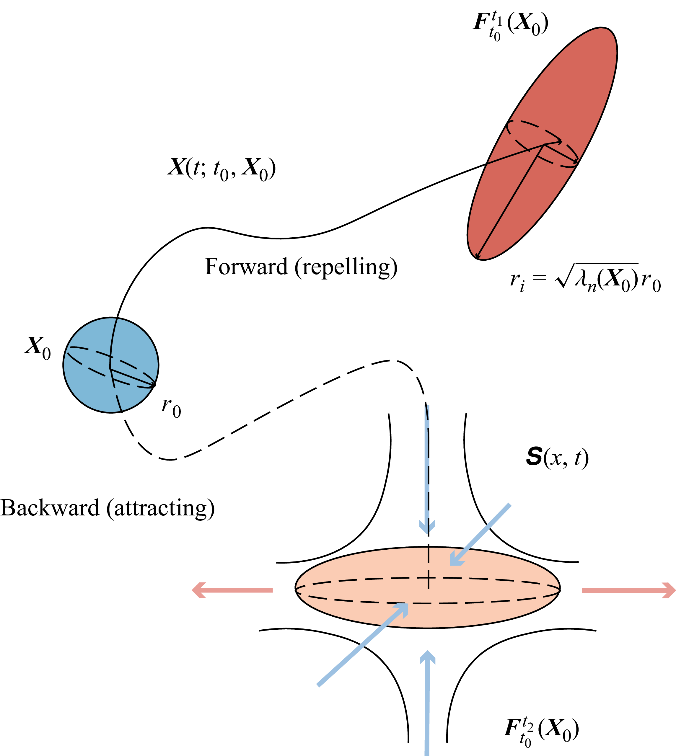
In this definition, the largest possible stretching at a point $\boldsymbol{X}_0$ is given by $\sqrt {\lambda _n(\boldsymbol{X}_0)}$ , where $\lambda _n$ is the largest eigenvalue of $C(\boldsymbol{X}_0)$ , with $n=3$ for 3-D flows. As a geometrical illustration, a material sphere with infinitesimally small radius $r_0$ initialised at $t_0$ is assumed to be transported by a 3-D flow (see figure 5). The sphere deforms into a small ellipsoid, which represents the change of local strain state $ \unicode{x1D64E}(x,t)$ in the flow field. The length of the $i$ th principal axis of the sphere is $\sqrt {\lambda _i(X_0)}\ (i=1,2,3)$ multiplied by the radius of the initial sphere.

Figure 5.

Schematics of the deformation of a fluid parcel. Two types of Lagrangian trajectories $F^t_{t_0}(\boldsymbol{X}_0)$ are illustrated. Forward tracking (solid line, $t_1\gt t_0$ ) detects ‘repelling’ Lagrangian structures, while backward tracking (dashed line, $t_2\lt t_0$ ) detects ‘attracting’ ones. The Lagrangian deformation, e.g. stretching (the light orange arrows) or compression (the light blue arrows), is the integral effects of local strain rate $ \unicode{x1D64E}(x,t)$ .

In practice, integrating trajectories forwards in time ( $t_1\gt t_0$ ) may produce FTLE ridges that mark the locations of repelling Lagrangian coherent structures. If the FTLE is calculated by integrating trajectories backwards in time ( $t_2\lt t_0$ ), then ridges in the FTLE field may indicate attracting material lines or attracting Lagrangian coherent structures. Examples of attaining ‘attracting’ structures through backward tracking can be found in the literature (see e.g. Green, Rowley & Haller Reference Green, Rowley and Haller2007; Zhao, Yang & Chen Reference Zhao, Yang and Chen2016). Hairpin vortices are detected for temporally developing channel flows in these studies. In the present study, the forward tracking method is employed for the spatially evolving structures in all cases to avoid determining the positions of flow structures in advance.

3.1. Co-existence of wave and vortex structures

We begin with the visualisation of the instantaneous flow field to offer an intuitive picture of the co-existing state of coherent structures in the mixing region. Furthermore, we will initiate the qualitative description of the wave–vortex relation, incorporating fundamental flow events such as lift-up. The Taylor frozen hypothesis is employed to deduce the underlying dynamical process from the spatial evolution of flow structures.

Figure 6(a) is an oblique view of the 3-D flow structures, which display the growth and metamorphosis of both disturbance waves (represented by positive conditioned normal velocity field $v$ ) and vortical structures (identified by the second invariant of velocity gradient $Q=1/4\omega _i\omega _i-1/2S_{ij}S_{ij}$ ) from inlet to the downstream regions. The normal velocity under the positive condition is defined as

(3.1) \begin{align} v^p_c(x,z) = \left \{ \begin{array}{ll} v(x,y_c,z) & \text{if } v\gt 0, \\ 0 & \text{if } v \leqslant 0, \end{array} \right . \end{align}

in which $y_c$ is the vertical coordinate of the mixing layer centreline. Similarly, the negatively conditioned normal velocity is defined as

(3.2) \begin{align} v^n_c(x,z) = \left \{ \begin{array}{ll} v(x,y_c,z) & \text{if } v\lt 0, \\ 0 & \text{if } v \geqslant 0. \end{array} \right . \end{align}

Figure 6.

Spatial distribution of the perturbation waves and vortices in Case1. The wave structures are visualised by iso-surfaces of the conditioned normal velocity at the plane $y_c=0.08$ , which is located approximately at the mixing layer centre. The vortex structures are represented by iso-surfaces of the second invariant of velocity gradient tensor, i.e. $Q=8\times 10^{-3}$ . (a) Oblique view of the 3-D flow structures. (b) Top-down view with the normal velocity positively conditioned. (c) Bottom-up view with the normal velocity negatively conditioned. The conditioned normal velocity fields in (a), (b) and (c) are magnified 30 times in scale.

Figure 6(b,c) show respectively a top-down view and a bottom-up view of the flow structures in the same region as figure 6(a), where wave structures are again visualised by either a positively or negatively conditioned normal velocity field. Initially, the vortex tubes near the inlet boundary are primarily in a 2-D form and rapidly become wavy due to the mode resonance of the oblique waves. Then the wavy spanwise vortex filaments either lift up or sweep down, and are stretched into staggered $\varLambda$ -shaped vortices (marked by black arrows) as they are convected downstream, with a passing spatial period of approximately one wavelength of the most unstable oblique mode from linear stability analysis. The $\varLambda$ -vortices further deform into hairpin-shaped vortices (labelled by black arrows) and finally break up into smaller-scale structures.

In the region farther away from the inlet, the relative positions of the wave and vortical structures become much clearer, e.g. at the streamwise position $x=50$ (labelled by a black arrow). The 3-D waves, characterised by the conditioned normal velocity, appear between the two legs of the $\varLambda$ -vortices. As the structures move downstream, the disturbance wave no longer appears as a 3-D wave bulge but is split into two branches that correspond to the adjacent legs of $\varLambda$ -vortices (see red arrows in figure 6). However, the wave structures, along with the accompanying vortical structures, persist in their downstream movement.

Depicted in figure 7(a–d) are contours of streamwise vorticity overlaid on velocity vectors $(v,w)$ within the slices at four subsequent streamwise locations, which reveal a possible causal relation between local flow events and vortex evolution. For instance, few vortical motions are observed in figure 7(a) despite the presence of relatively small streamwise vorticity. The slice in figure 7(b) cuts through the first set of $\varLambda$ -vortices. In this region, the positive normal fluid motion within $\varLambda$ -vortex 1, and the negative normal motion between $\varLambda$ -vortex 1 and $\varLambda$ -vortex 2, sustain the local vortical structures. The connection between the normal fluid events and vortex structures is similar to that in the turbulent bursting of wall-bounded flow, i.e. the ‘lift-up’ and ‘sweep-down’ events sustaining the existence of streaks. It should be noted that in turbulent bursting of wall bounded flows, the sweep events happen passively as the lift-up events cause momentum loss near the wall. However, in the mixing layer, the lift-up and sweep-down in either positive or negative normal directions is permitted, as there is no wall restriction in the current configuration (this will be discussed in detail in § 5). In figure 7(c), the lift and sweep events, along with vortical motions, are further enhanced. A much stronger nonlinearity effect leads to the breakdown of vortices in figure 7(d), which indicates that the flow is gradually evolving into a turbulent state.

Figure 7.

Evolution of streamwise vortical structures in $z$ – $y$ slices at a sequence of streamwise positions: (a) $x=16$ , (b) $x=85$ , (c) $x=110$ , and (d) $x=227$ , as shown in figure 6 labelled by I, II, III and IV, respectively. The contours are for the streamwise vorticity, while the vectors represent the combination of normal velocity $v$ and spanwise velocity $w$ .

In addition to the results presented above, the visualisation of a wave/vortex co-existence state under a different condition is also carried out to explore the effects of random disturbance at the inlet. For clarity, the results and corresponding discussions will be published separately in another paper.

3.2. Co-evolution of wave and vortex structures

In this subsection, the spatiotemporal evolutions of both the wave and vortex structures are explored by involving Lagrangian elements driven by the same instantaneous Eulerian fields of Case1. This analysis can help to provide insights into the dynamics of different coherent structures.

Displayed in figure 8 are four sets of timelines (i.e. the ‘digital hydrogen bubbles’ $\boldsymbol{L}(t)$ ), which are initially released at different streamwise locations ( $x_0 = 50$ , 100 and 200) with a constant release time interval. It should be mentioned that the timelines only span a range $z \in [5.0,30.9]$ in the $z$ -direction to save tracking time.

Figure 8.

Timelines released simultaneously at the same normal position ( $y_0=0.18$ ) but with different streamwise locations: (a) $x_0=50$ , (b) $x_0=100$ , (c,d) $x_0=200$ . The timelines are coloured by the local normal position $y$ of particles to visualise the spatial metamorphosis of material lines caused by the local flow structures. Note that (d) presents the same timelines as (c) but with the $y$ -axis inverted.

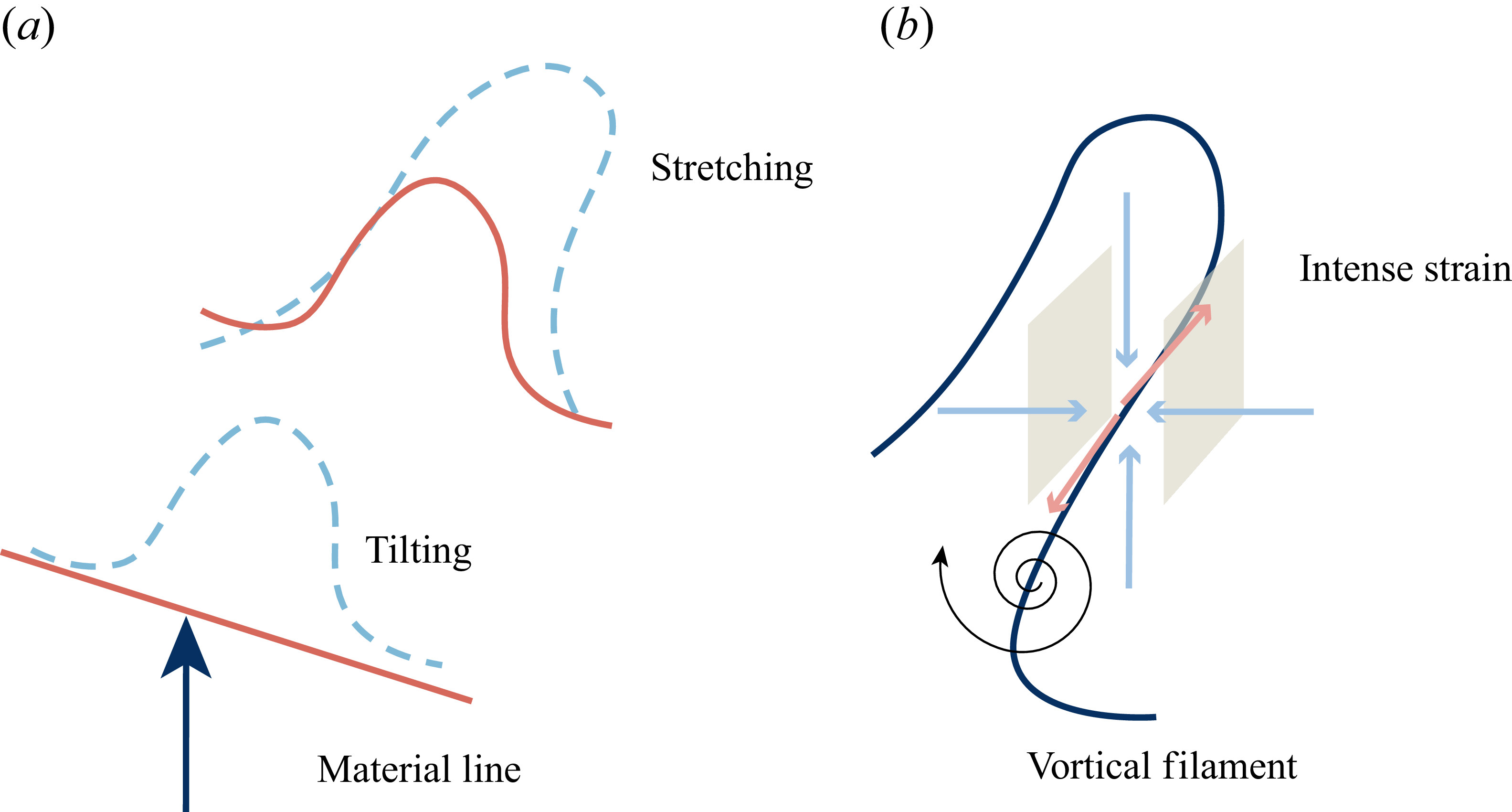
The first set of timelines is obtained by releasing at $x=50$ , which evolves into a wave-like staggering pattern as shown in figure 8(a). The streamwise and spanwise distances between the adjacent ‘peaks’ or ‘valleys’ of 3-D waves are approximately 20 and 15, respectively. The amplitudes of the wavy bulges gradually increase in both of the normal directions (see the variation of the colour bars). Furthermore, the timelines in front of the bulge are denser than those in other regions, which results from the deficit of streamwise velocity. In this region, the evolution of material lines is mainly controlled by the tilting mechanism, as illustrated in figure 9(a). Depicted in figure 8(b) are another set of timelines released at $x=100$ . As staggered wavy bulges start to deform, their amplitudes are further magnified. Figure 8(c,d) show timelines released much further downstream at $x=200$ , where the material lines appear inclined and twisted, indicating that $\varLambda$ - or hairpin-shaped vortex patterns become significantly dominant. Figure 8(d) presents an upside-down version of the timeline in figure 8(c), indicating that hairpin vortices grow on both sides of the mixing centre layer in the normal direction, which differs from boundary layers and will be discussed later.

Figure 9.

Illustration of (a) tilting and stretching of a material line, and (b) stretching of a vortical filament.

Particles are not simply oscillating upwards or downwards, but concentrate into inclined ribs through vortex stretching mechanism (as illustrated in figure 9 b). Due to stronger vortical motions, the particle concentration is observed to be more rapid and compact in figure 8(c,d) than in figure 8(b).

Figure 10 shows evolutions of the material surface $\boldsymbol{M}(t)$ superimposed with the iso-surface of the second invariant of velocity gradient $Q$ at different time $t$ . As illustrated by the Eulerian patterns in § 3.1, we know that the initial shear layer (homogeneous in streamwise and spanwise directions) is susceptible to redistribution and deformation due to the presence of 3-D disturbance waves and vortical structures, as evidenced by the wrinkling Lagrangian structures. From figure 10(a–c), the general process for a 3-D perturbation wave to trigger the development of hairpin vortices can be described as follows.

Figure 10.

Evolution of a material surface (in black and white) initiated at $y_0=0,\ x_0 \in [5,35],\ z_0 \in [5,30]$ for Case1: (a,d) $t-t_0=10.0$ , (b,e) $t-t_0=43.5$ , and (c,f) $t-t_0=98.0$ . (a–c) The iso-surfaces of $Q=4\times 10^{-3}$ are superimposed and coloured by the streamwise velocity $u$ ; the colour map at the top-left corner of each panel reflects the values of normal coordinate $y$ . (d–f) The same $Q$ iso-surfaces are visualised in grey, and the colour map represents the FTLE field $\varLambda _{t-T}^t$ for material surfaces at $t$ with fixed integration time $T=2$ .

Shown in figure 10(a) is the instantaneous shape of a material surface near the inlet, where the material surface undergoes subtle normal deformation, indicating that the staggered 3-D wave structures are dominant in this region. The wavy vortical structures in the same region are large-scale spanwise vortex tubes, which are the result of motion of 3-D disturbance waves. The amplitude of the 3-D waves increases as the material surface moves downstream (see figure 10 b). This increase in amplitude is consistent with the fluid lift-up or sweep-down events shown in figure 6. At this stage, $\varLambda$ -vortices form, with their two legs embracing a single 3-D wave.

With continuous deformation of the material surface, the 3-D bulge no longer maintains its original shape but splits into two ‘peaks’ in the spanwise direction (see arrows in figure 10 b). This phenomenon can serve as evidence that the lateral motions from vortical flows are strong enough in this region. As the flow structures continue to develop downstream, the $\varLambda$ -vortices have gradually evolved into hairpin-shaped structures in this region. It becomes almost impossible to distinguish between the material surface and the Eulerian vortical structures, as nearly all particles engage with neighbouring vortical structures (see figure 10 c).

3.3. Wave–vortex interactions

In § 3.1, it is observed that the transitional section of the mixing layer is dominated by both wave and vortex structures. In § 3.2, it is further explained that the two types of structures evolve with a coupling mechanism. In the early stage of transition, the wave–vortex relation is assumed to be causal rather than merely correlated. In this subsection, evidence will be presented to further demonstrate that the wave and vortex structures interact with each other through local strain rate fields. The target is realised by tracking relevant quantities by interpolating local flow information onto an evolving material surface.

Depicted in figure 10(d–f) are evolutions of the FTLE field as introduced in § 2.3, which measures the innate deformation of a material surface. The scalar field is carried by the same material surface $\boldsymbol{M}(t)$ as shown in figure 10(a–c) and evaluated in § 3.2. Through the forward integration as introduced in § 2.3, ‘repelling’ Lagrangian structures are obtained, which are represented by the local maximum magnitude of FTLE fields. The local maximum can be seen as ridges on the material surface and labelled by the coloured arrows in these figures. At the early stage of transition (see figure 10 d), one local maximum of the FTLE is observed encircling the ‘mountainside’ of the 3-D wave (labelled by the black arrow), with another local maximum on the ridges connecting neighbouring wave peaks (labelled by the red arrow). Global maxima occur at valleys between wave peaks, indicating that the stretching is most intense in these areas. In figure 10(e), part of the local maxima of FTLE migrate to the ‘mountain flanks’ of the wave peaks (labelled by the yellow arrows). These regions on $\boldsymbol{M}(t)$ are also places where the legs of inclined $\varLambda$ -vortices penetrate the material surface, implying that the local maxima of the FTLE are indeed projections of the detected ‘repelling’ Lagrangian structures ( $\varLambda$ -vortices herein). In figure 10(f), the maxima of the FTLE appear on boundaries of the vortices (labelled by the orange arrows), which represent vortex stretching on the rotation edges. Additionally, particles distributed within the ‘bulge’ zones are found much less in this stage because those particles have been causally attracted into vortical structures. It should be noted that the number of particles used for Lagrangian tracking is insufficient. If a sufficiently large number of particles are continuously injected, the ‘bulge’ region should appear as a continuous surface.

The above analysis unveils the kinematic stretching and deformation of Lagrangian structures. However, it is also appealing to consider what happens in the neighbourhood of the 2-D surface in 3-D space, where high strain rate layers may function as a ‘catalyst’ by dynamically interacting with both the waves and vortices. Displayed in figure 11(a–d) are distributions of the strain rate related quantities on the material surface. It is found that higher $S_{12}=1/2(\partial u/\partial y + \partial v/\partial x)$ appears on the ‘hillsides’ of wave packets, especially on the wave-front regions (labelled by black arrows). Both $S_{13}=1/2(\partial u/\partial z + \partial w/\partial x)$ and $S_{23}=1/2(\partial v/\partial z + \partial w/\partial y)$ are observed to be concentrated in the wave-flank zones (labelled by red arrows) but in opposite strain directions. In addition, it turns out that the distribution of $S_{12}$ is most similar to that of the magnitude $|\unicode{x1D64E}|$ by comparing different components of the strain rate tensor ( $S_{12}$ , $S_{12}$ and $S_{23}$ ) with $|\unicode{x1D64E}|$ . The large magnitude of the strain rate also indicates a high dissipation rate in such regions. Figure 11(e) displays the flux contribution by stretching to the change of enstrophy. The distribution of $\boldsymbol{\omega }\boldsymbol{\cdot }\unicode{x1D64E}\boldsymbol{\cdot }\boldsymbol{\omega }$ is quite similar to that of $S_{13}$ or $S_{23}$ , indicating that the local strain rate field, induced by wave motions rather than vorticity self-induction, is an effective contributor to the formation of vortical structures in the early stage of transition.

Figure 11.

The material surface at $t-t_0=35$ , which is initiated at $y_0=0,\ x_0 \in [5,35],\ z_0 \in [5,30]$ for Case1 (same as in figure 10), and coloured by different components of the strain rate tensor: (a) $S_{12}$ , (b) $S_{13}$ , (c) $S_{23}$ , (d) $|\unicode{x1D64E}|$ , the norm of the strain rate tensor, and (e) $\boldsymbol{\omega }\boldsymbol{\cdot }\unicode{x1D64E}\boldsymbol{\cdot }\boldsymbol{\omega }$ , the stretching term of enstrophy.

It should be remarked that the geometric form of the material surface at this moment comes from the integrated effect of local strain and vorticity from the moment when the material surface is initially released. The dynamical process can be interpreted by the relation between Lagrangian and Eulerian stretching, which formulates as the evolution of the deformation gradient tensor $F_{ij}(t)=\boldsymbol{\nabla }F_{t_0}^t=\partial X_i(t,\boldsymbol{X}_0)/\partial X_{0j}$ :

(3.3) \begin{align} \frac {\text{d}F_{ij}(t)}{\text{d}t} = G_{ik}(t)\,F_{kj}(t) = (S_{ik} + A_{ik})\,F_{kj}(t), \end{align}

in which $G_{ik}$ is the velocity gradient tensor, which can be decomposed into a symmetric part (i.e. the strain rate tensor $S_{ij}$ ) and an antisymmetric part (i.e. the rotation tensor $A_{ij}$ ). Equation (3.3) suggests that the deformation of the material surface is controlled by both strain and rotation parts of the velocity gradient, even though in the early stages of the evolution (see figure 10 a,b), it undergoes more metamorphosis due to the straining effect, while the rotation becomes stronger and causes a single wave peak to break into two parts at later stages (see figure 10 c,d), as will be discussed later.

Based on the above results, the process where a 3-D wave interacts dynamically with adjacent $\varLambda$ -vortices (see figure 12 a) through immediate high shear (strain rate) structures (figure 12b) can be interpreted as follows. Ejection of fluids (termed as a 3-D perturbation wave in figure 12a,b) alters the motion of local fluids, which should be substantially convected downstream. Surrounding the 3-D wave ‘mountain’ (represented by the meshed surface in the illustration), the fluids originating from upstream (straight solid arrows) are obstructed on the ‘windward’ side, and experience a decrease in streamwise velocity. The decelerated fluids either participate in the ejection process or circumvent the wave (straight dashed arrows). Furthermore, mass conservation requires that the position vacated by the injected fluids must be filled by fluids from the ejection terminus. These reverse motions lead to the formation of a high-shear layer with enhanced vorticity concentration. As illustrated in figure 12(b), the sketched local strain rate field on the ‘windward’ side is dominated by the high-shear components $\partial v/\partial x$ and $\partial u/\partial y$ , which correspond to high magnitude of $S_{12}$ in this region. Similarly, at the peak of the 3-D wave where $\partial v/\partial x$ becomes weak, the shear component $\partial u/\partial y$ along with lateral stretching makes spanwise vorticity concentrated in this region, which explains the formation of a $\varLambda$ -vortex head. At flanks of the 3-D wave, an ejecting/sweeping event causes high shear $\partial v/\partial z$ , while the spanwise gradient of $u$ causes high shear $\partial u/\partial z$ , which gives rise to the large magnitudes of $S_{23}$ and $S_{13}$ , respectively. It is worth noting that the initial high-vorticity blobs (sketched by swirling arrows) are born in the 3-D wave flanks especially due to the local shear $\partial v/\partial z$ (the main contribution to streamwise vorticity concentration). The blobs are further stretched by the global mean shear, which will be explained in § 4.2.

Figure 12.

Illustration of (a) local motion of fluids around a 3-D wave, and (b) strain rate state around a 3-D wave.

4.1. Energy evolution

The streamwise evolutions of kinetic energy in Fourier modes of Case1 are calculated to statistically investigate the dynamic growth of disturbance waves, which have been visualised by material surfaces in § 3.2. The temporal–spatial kinetic energy spectrum can be defined in the form

(4.1) \begin{align} E(\omega ,\beta )=\int _{-L_y/2}^{L_y/2} \tilde {u}(\omega ,\beta )\, \tilde {u}^c(\omega ,\beta )\,\text{d}y, \end{align}

where the superscript ‘c’ denotes the complex conjugate. The streamwise evolutions of the frequency spectrum and wavenumber spectra are shown in figures 13(a) and 13(b), respectively. As is seen in figure 13(a), the kinetic energy is concentrated and distributed near the fundamental frequency $\omega _0=0.41$ of disturbance waves. High-order harmonic frequencies $3/2\omega _0$ and $5/2\omega _0$ gradually come into being due to wave resonance during the very early stage of transition ( $x\lt 50$ ). It can also be observed that the kinetic energy is mainly concentrated at the wavenumber $\beta _0=0.36$ of oblique disturbance. Harmonic wavenumbers such as $2\beta _0$ and $3\beta _0$ become important where $x\gt 100$ , as shown in figure 13(b). For those high-order harmonic spanwise structures, the third harmonic wave increases most rapidly, and becomes secondary to the fundamental wavenumber within the region $100\lt x\lt 400$ . Much farther downstream, the spectral energy gradually spreads into a wider wavenumber range, although the mode with the fundamental frequency and wavenumber still dominates.

Figure 13.

Streamwise evolutions of spectral kinetic energy $E(\omega ,\beta )$ : (a) frequency spectrum at $\beta =\beta _0$ , (b) spanwise wavenumber spectrum at $\omega =\omega _0$ , and (c) spectral energy of selected modes. Here, the frequency and spanwise wavenumber spectra are rescaled by those of the fundamental mode $E(\omega _0, \beta _0)$ at the inlet.

To investigate the mode–mode energy competition, the evolutions of spectral kinetic energy for several selected Fourier modes from figures 13(a) and 13(b) are shown in figure 13(c). It is suggested that the growth of energy in these selected modes could be generally divided into three stages. In the first stage ( $0\lt x\lt 50$ ), i.e. the region very close to the inlet, energy of all modes experiences a transient increase, except that of the 2-D disturbance mode $(1,0)$ , which undergoes a rapid increase first and then decreases. In the following stage ( $50\lt x\lt 150$ ), the energy of the 3-D oblique mode $(1,1)$ and 2-D disturbance mode $(1,0)$ both grow slowly. The energy of the mode with frequence $(3/2,1)$ increases in a similar way to the $(1,1)$ mode. Other high-order harmonic modes such as $(1,2)$ and $(1,3)$ also experience growths in the second stage, which are much more rapid than the fundamental modes.

The energy evolutions examined above indicate that the excitation of 3-D disturbances with the 2-D field would eventually establish a positive feedback loop and lead to the self-sustained simultaneous growth of 2-D and 3-D waves. The final stage of energy development ( $x\gt 150$ ), shown in figure 13(c), is characterised by much more moderate growth, and the energy contained in each mode tends to be the same order of magnitude. Meanwhile, the wave–vortex interaction begins at approximately $x=150$ due to the appearance of a $\varLambda$ -vortex (accompanied by surges of high-order harmonic modes of $(1,2)$ or $(1,3)$ ). This is consistent with the visualisation in figure 6 or figure 10, indicating that nonlinear effects become dominant in this region.

From the perspective of energy feedback, the 3-D wave mode $(1,1)$ takes the lead in energy growth within the range $50\lt x\lt 150$ , during which localised high shear emerges due to the amplification of 3-D waves. The 2-D wave mode $(1,0)$ excites strong energy transfer from the mean flow into the 3-D wave since its amplitude is sufficiently large initially (see e.g. Croswell Reference Croswell1985; Herbert Reference Herbert1988). While some portions of this excited energy increase the amplitude of mode $(1,1)$ , other parts are dissipated during the evolution. Once the energy of mode $(1,1)$ attains a sufficiently large value ( $x\gt 50$ ), the energy of mode $(1,0)$ shows a tendency for slow increase again.

It needs to be pointed out that the evolutions of energy spectra in figure 13 are indeed a time-averaged result. The streamwise wavy phenomenon of these single-mode energy spectra comes from periodic structures in that dimension. The averaging operation remarkably reduces streamwise oscillation of the energy spectra for modes $(1,0)$ and $(1,2)$ , while inconspicuously flattening other modes because these modes are travelling with different phase velocities.

4.2. Formation of streamwise vorticity

In addition to the growth of wave energy, it is also necessary to analyse the dynamical process through which the oblique waves trigger the formation of $\varLambda$ -vortices as visualised in § 3.3. To achieve this, the flow field is decomposed into a mean component and a fluctuating component to distinguish the wave part from other aspects of flow, i.e.

(4.2) \begin{align} \begin{aligned} & \boldsymbol{u}(\boldsymbol{x},t)=\boldsymbol{U}(\boldsymbol{x},t) + \tilde { \boldsymbol{u}}(\boldsymbol{x},t),\\ & \boldsymbol{\omega }(\boldsymbol{x},t)=\boldsymbol{\varOmega }(\boldsymbol{x},t) + \tilde {\boldsymbol{\omega }}(\boldsymbol{x},t). \\ \end{aligned} \end{align}

By substituting the above decomposition into the dynamic equation of vorticity (2.12), one can obtain the governing equations of both mean vorticity and fluctuating vorticity. Detailed derivations for these equations are given in Appendix B. The interaction between disturbance and vorticity can be represented by terms in right-hand side of the disturbance vorticity equation (B2). Here, the focus is placed on contributions to the change in streamwise vorticity from fluctuating vortex stretching by the mean strain rate $(\tilde {\boldsymbol{\omega }} \boldsymbol{\cdot }\boldsymbol{\nabla }) \boldsymbol{U}$ , and mean vortex stretching by fluctuating strain rate $(\boldsymbol{\varOmega } \boldsymbol{\cdot }\boldsymbol{\nabla })\tilde {\boldsymbol{u}}$ :

(4.3) \begin{align} \frac {\partial \tilde \omega _x}{\partial t} \sim {}& \tilde \omega _x\dfrac {\partial U_x}{\partial x} + \tilde \omega _{y}\dfrac {\partial U_x}{\partial y} + \tilde \omega _z\dfrac {\partial U_x}{\partial z}\notag \\ & {}+\varOmega _x\dfrac {\partial \tilde u_x}{\partial x} + \varOmega _y \dfrac {\partial \tilde u_x}{\partial y} + \varOmega _z\dfrac {\partial \tilde u_x}{\partial z}. \end{align}

The right-hand side of (4.3) can be divided into two parts, i.e. stretching/bending of the fluctuating vorticity by the mean velocity field, and stretching/bending of the mean vorticity by the fluctuating velocity field. Shown in figure 14 are streamwise fluxes of the six terms in (4.3), which are calculated by a surface integral over $y$ – $z$ slices at each $x$ position. Note that these terms are integrated within a region (denoted by $I$ ) that covers one leg of the streamwise vortex pair.

Figure 14.

Streamwise evolution of the right-hand-side contributions of the governing equation for fluctuating vorticity: (a) stretching and twisting of the fluctuating vortex by the mean flow field, and (b) stretching and twisting of the mean vortex by the fluctuating velocity field. Here, $I$ denotes the region of the streamwise flux integral.

As discussed previously, 3-D waves are introduced as inflow disturbance, and their growth is correlated with mode interactions. Now we further demonstrate the direct consequence of disturbance wave amplification in figure 14, i.e. the creation of $\varLambda$ -vortices in locally disturbed strain rate fields. It is also demonstrated that the high-shear layers with enhanced vorticity are generated by interaction of waves with the mean flow. Figure 14 shows that the primary contribution to the generation of streamwise vorticity in the region $x\lt 50$ comes from $\tilde \omega _x (\partial U_x/\partial x)$ (solid line in figure 14 a) and $\varOmega _z(\partial \tilde u_x/\partial z)$ (dot-dashed line in figure 14 b). The former represents the stretching of streamwise fluctuating vorticity by mean streamwise velocity gradient; this is the consequence of decrease in streamwise velocity caused by 3-D wave perturbation, as illustrated in figure 9(a). The latter comes from the tilting of mean spanwise vorticity $\varOmega _z$ by spanwise fluctuating shear $\partial \tilde {u}_x/\partial z$ , which is also the effect of the 3-D wave motion. Therefore, it is the wave property of $\tilde u_x$ with strong oscillations that results in the streamwise amplification of vorticity flux.

In the region $50\lt x\lt 120$ , contributions from other terms gradually increase, corresponding to the second stage of mode growth in figure 13. For example, as shown in figure 14(a), the tilting of spanwise vorticity fluctuation $\tilde \omega _z$ by mean shear $\partial U_x/\partial z$ (dot-dashed line) starts to be intensified. Meanwhile, the stretching of mean streamwise vorticity $\varOmega _x$ by fluctuating normal strain rate $\partial \tilde {u}_x/\partial x$ (solid line in figure 14 b) and the tilting of normal mean vorticity $\varOmega _y$ by fluctuating shear $\partial \tilde {u}_x/\partial y$ (dashed line in figure 14 b) are also enhanced. This indicates that the growth of perturbation waves leads to local redistribution of the strain rate field, and the shear parts of strain rate field give rise to quasi-streamwise vortex structures. In the region $x\gt 120$ , the evolution enters the nonlinear development stage and tends to saturate downstream. This saturation can also be observed in the same region of figure 13, where different modes become equally competitive, and the turbulent motion is sustained by energy exchanges among these modes (Li et al. Reference Li, Peyvan, Ghiasi, Komperda and Mashayek2021).

4.3. Role of high strain rate

Based on the analysis of wave–vortex interaction in § 3.3, it is found that fluid layers of high strain rate ( $S_{12}$ , $S_{13}$ , $S_{23}$ or $|\unicode{x1D64E}|$ ) are typically preserved surrounding the wave structure, which are the regions where vortex structures are nurtured (as illustrated in figure 12(c,d) and depicted in figure 11). According to (2.14), the production of enstrophy from vortex stretching/tilting is governed by the alignment between the vorticity vector and eigenvectors of the strain rate tensor $\beta _i\cos ^2 \langle {\boldsymbol \omega ,\boldsymbol \varLambda _i}\rangle$ . Since the dynamics of $ \unicode{x1D64E}$ and $\boldsymbol{\omega }$ are coupled with each other, the conditional statistics of the preferential alignment upon the magnitude of strain rate tensor $|\unicode{x1D64E}|$ are carried out as a validation test.

As displayed in figure 15, the probability density function (p.d.f.) of the cosine of the angle between the vorticity vector and intermediate eigenvector ( $\cos \langle \boldsymbol \omega ,\boldsymbol \varLambda _2\rangle$ ) shows strong peaks at $1$ and $-1$ , indicating that the most likely behaviour involves considerable alignment with $\langle \boldsymbol \omega ,\boldsymbol \varLambda _2\rangle =0^\circ$ and $180^\circ$ . This observation is consistent with the findings in homogeneous shear turbulence (Ashurst et al. Reference Ashurst, Kerstein, Kerr and Gibson1987) and stratified shear turbulence (Jiang et al. Reference Jiang, Atoufi, Zhu, Lefauve, Taylor, Dalziel and Linden2023). Meanwhile, the corresponding p.d.f.s of $\cos \langle \boldsymbol \omega ,\boldsymbol \varLambda _i\rangle$ conditioned on $|\unicode{x1D64E}|^2\gt \langle |\unicode{x1D64E}|^2\rangle$ are calculated to highlight the effect of high strain rate, where $\langle |\unicode{x1D64E}|^2\rangle$ is the averaged stain rate value over the entire domain for statistical analysis. It turns out that the preferential alignments increase with the strength of strain rate in both selected regions (figure 15 a,b), suggesting that turbulence is more easily generated in high strain rate regions. By comparing figures 15(a) and 15(b), it is found that the margin p.d.f. of $\cos \langle \boldsymbol \omega ,\boldsymbol \varLambda _2\rangle$ (within either $[0.9,1.0]$ or $[-1.0,-0.9]$ ) is steeper in figure 15(a) than in figure 15(b), indicating that the preferential alignment of $\mathbf \varLambda _2$ in the wave–vortex interaction stage ( $150\lt x\lt 220$ ) is weaker than that in the wave growth stage ( $50\lt x\lt 120$ ). It is also observed that the effect of high strain rate, which leads to more preferential alignment between the intermediate eigenvector and the vorticity vector, is more pronounced in the region $50\lt x\lt 120$ .

Figure 15.

The p.d.f.s of the cosine of the angle between the vorticity vector $\mathbf{\omega }$ and eigenvectors $\mathbf \varLambda _{i}$ of the strain rate tensor within two selected regions: (a) $50\lt x\lt 120$ and (b) $150\lt x\lt 220$ . Lines with symbols represent the p.d.f.s conditioned on the strength of strain rate $|\unicode{x1D64E}|^2\gt \langle |\unicode{x1D64E}|^2\rangle$ .

It is also appealing to consider the effect of high strain rate on the production of enstrophy $\boldsymbol{\omega }^\textrm{T} \unicode{x1D64E}\boldsymbol{\omega }$ (or $\omega _i \omega _j S_{ij}$ ) and production of strain rate $S_{ij}S_{jk}S_{ki}$ within the two selected regions. Depicted in figure 16(a,b) are p.d.f.s and conditional p.d.f.s (upon the strain rate) of the two terms. These distributions are all positively skewed, indicating a net production of both enstrophy and strain rate from the early stage of transition to the late stage of flow development. Conditional samplings of $\omega _i \omega _j S_{ij}$ and $-({4}/{3})S_{ij}S_{jk}S_{ki}$ on high strain rate ( $|\unicode{x1D64E}|^2\gt 2\langle|\unicode{x1D64E}|^2\rangle$ ) reveal that both quantities become more intermittent and more positively skewed (the variations are marked by a black arrow). It is further identified that the ratio of $\omega _i \omega _j S_{ij}$ to $-S_{ij}S_{jk}S_{ki}$ is consistent with the reported value $4/3$ for homogeneous isotropic turbulence (Lawson & Dawson Reference Lawson and Dawson2015).

Figure 16.

The p.d.f.s of $\omega _i \omega _j S_{ij}$ and $-({4}/{3})S_{ij}S_{jk}S_{ki}$ within two selected regions: (a) $50\lt x\lt 120$ and (b) $150\lt x\lt 220$ . The p.d.f.s conditioned on high strain rate are also plotted for comparison.

By comparing figures 16(a) and 16(b), it is found that the generations of enstrophy and strain rate are relatively weak during the early transition phase ( $50\lt x\lt 120$ ), but increase approximately by four times in the late transition stage ( $150\lt x\lt 220$ ). The reason for this phenomenon lies in the enhancement of the stretching term as highlighted in figure 10(d–f). Furthermore, it is observed that the p.d.f.s become a little more ‘symmetric’ downstream, which could be the consequence of nonlinearity. These conditional results underscore that enstrophy tends to be generated in regions of intense strain rate, even though the localised enhancement in strain originates from the motion of 3-D waves.

4.4. Effect of convective Mach number

To shed light on the effect of compressibility upon the spatial development of a transitional mixing layer, statistical studies are conducted for the test case with convective Mach number $Mc=1.4$ . Shown in figures 17(a) and 17(b) are the streamwise variations of stretching and twisting of the fluctuating vortex by the mean flow field, and stretching and twisting of the mean vortex by the fluctuating velocity, respectively. It turns out that the mixing layer grows at a lower frequency (i.e. the quasi-periodic structures have larger wavelength) in comparison with the case $Mc=0.7$ . Analogous to the situation at $Mc=0.7$ , the primary contribution to the generation of streamwise vorticity in the early transition region ( $x\lt 75$ ) still comes from $\tilde \omega _x (\partial U_x/\partial x)$ (solid line in figure 17 a) and $\varOmega _z(\partial \tilde u_x/\partial z)$ (dot-dashed line in figure 17 b). Besides, contributions from other terms gradually increase in the region $75\lt x\lt 150$ , and the evolution enters the nonlinear development stage after $x\gt 150$ , similar to the case $Mc=0.7$ . The main difference lies in the tilting of the mean spanwise vorticity by spanwise fluctuating shear $\varOmega _z(\partial \tilde u_x/\partial z)$ , which is even stronger than that in the low convective Mach number case. This phenomenon actually confirms the dominant role of oblique instability in the high convective Mach number regime (Sandham & Reynolds Reference Sandham and Reynolds1991).

Figure 17.

Streamwise evolution of the right-hand-side contributions of the governing equation for fluctuating vorticity at the convective Mach number $Mc=1.4$ : (a) stretching and twisting of the fluctuating vortex by the mean flow field, and (b) stretching and twisting of the mean vortex by the fluctuating velocity field. Here, $I$ denotes the region of the streamwise flux integral.

Depicted in figures 18(a) and 18(b) are p.d.f.s of the alignment between vorticity vector $\boldsymbol{\omega }$ and eigenvectors $\boldsymbol{\varLambda}_{i}$ of the strain rate tensor within two selected regions for the case $Mc=1.4$ . As can be seen, the p.d.f.s of the cosine of the angle between the vorticity vector and intermediate eigenvector ( $\cos \langle \boldsymbol \omega ,\boldsymbol \varLambda _2\rangle$ ) display an increased concentration near 1 and $-1$ in both selected regions. The increasing trend is even more pronounced in the downstream region, i.e. figure 18(b). It is also found that the effect of high strain rate on the preferential alignment is enhanced in the high Mach number case compared to the low Mach number case.

Figure 18.

The p.d.f.s of cosine of the angle between vorticity vector $\boldsymbol{\omega }$ and eigenvectors $\boldsymbol{\varLambda}_{i}$ of the strain rate tensor within two selected regions at the convective Mach number $Mc=1.4$ : (a) $50\lt x\lt 150$ and (b) $200\lt x\lt 300$ . Lines with symbols represent the conditional p.d.f.s based on the strength of strain rate $|\unicode{x1D64E}|^2\gt \langle |\unicode{x1D64E}|^2\rangle$ .

Figures 19(a) and 19(b) present the p.d.f.s of enstrophy production $\omega _i \omega _j S_{ij}$ and strain rate production $-({4}/{3})S_{ij}S_{jk}S_{ki}$ within two selected regions for the case $Mc=1.4$ . Basically, the production in both regions decreases by $2/3$ compared with that in the case $Mc=0.7$ . Comparisons of conditioned samplings show that the influence of Mach number on the strain rate contribution is limited.

Figure 19.

The p.d.f.s of enstrophy production $\omega _i \omega _j S_{ij}$ and strain rate production $-({4}/{3})S_{ij}S_{jk}S_{ki}$ within two selected regions at the convective Mach number $Mc=1.4$ : (a) $50\lt x\lt 150$ and (b) $200\lt x\lt 300$ . The p.d.f.s conditioned on high strain rate are also plotted for comparison.

5.1. A comparison with the scenario in boundary layer flow

Inspired by the hypothesis on the role played by 3-D waves in boundary layer transition (Lee & Wu Reference Lee and Wu2008; Jiang et al. Reference Jiang, Lee, Chen, Smith and Linden2020a ), it is suggested that these wave structures serve as pivotal building blocks in laminar–turbulent transition of a compressible mixing layer flow. Jiang et al. (Reference Jiang, Lefauve, Dalziel and Linden2022) also highlighted that the amplification of a 3-D wave as a key initiator of a vortex may be a universal feature of shear-driven turbulence, occurring in both wall-bounded and wall-free configurations.

Although the present study demonstrates a similar role of a 3-D wave in the transition of a mixing layer, it should be noted that the dynamic process for a mixing layer can differ from that for a boundary layer. This discrepancy arises because 3-D waves are allowed to move freely in both vertical directions in the mixing layer, as opposed to being constrained to an impermeable wall. Given a disturbance with the spanwise wavelength $\lambda _d$ , both the wave and hairpin vortex structures are antisymmetric in the $z$ -direction between the upper and lower parts of the mixing layer (see figure 20 a). There are two heads (one is on the high-speed side, and the other is on the low-speed side) and four legs (two of them on the high-speed side, and the other two on the low-speed side) within one period of the disturbances. However, given a disturbance with the same spanwise wavelength $\lambda _d$ , the wave and hairpin vortex structures are symmetric in the flat plate boundary layer. There are one head and two legs within one period of the disturbances (see figure 20 b).

As a consequence of interaction with the mean shear, disturbances provide aid in triggering the generation of quasi-streamwise vortices and hairpin vortices in the high- and low-speed fluid layers, respectively. Vortices adjacent to each other at different layers, with their heads oreiented in opposite spanwise directions, can be connected by their legs. However, hairpin vortices with a consistent orientation predominate in boundary layer flows. Furthermore, the presence of walls in the boundary layer results in the isolation of quasi-streamwise vortices, with the potential for their legs to interact with each other (e.g. reconnection), while the lifting phenomenon primarily occurs above the hairpin neck (see Zhou et al. Reference Zhou, Adrian, Balachandar and Kendall1999). It should also be mentioned that the vertical lifting of vortices within the mixing layer may experience suppression to some extent due to the presence of stratification. For example, Jiang et al. (Reference Jiang, Lefauve, Dalziel and Linden2022) demonstrated that the vertical inclination angle for a hairpin vortex in stratified mixing layers is approximately $10^\circ$ , which is approximately half of what is observed in the present study.

5.2. The 3-D wave and ejection/sweep of fluids

In § 3.2, visualisation of typical material surfaces exhibits a continuous metamorphosis from the initially 2-D vortex tubes near the inlet to downstream wavy structures and the consequent staggered $\Lambda$ -shaped vortices. This reveals a causal relationship between local flow events, characterised by positive and negative vertical fluid motions, and the persistence of vortical structures. In figures 6, 10 and 11, one can clearly observe the localised normal fluid movements, which stem from perturbation ‘seeds’ introduced at the inlet, and germinate within the background shear.

The $Q2\ (u^{\prime}\lt 0, v^{\prime}\gt 0)$ and $Q4\ (u^{\prime}\gt 0, v^{\prime}\lt 0)$ motions, which are associated with the ejection and sweep events in wall-bounded flow, can similarly serve as a classification of gradient-type motions in the mixing layer. This enables the identification on contributions of the ejection and sweep events to vortex formation and turbulence production. By examining small flow structure units, which encompass individual wave/vortex structure and neighbouring flows, a quadrant analysis is conducted for velocity fluctuations $u^{\prime}$ and $v^{\prime}$ across different streamwise regions (see figure 21). To facilitate the differentiation of events occurring at different heights within the mixing layer, the scatter plots in figure 21 are colour-coded to represent deviations of the normal position from the mean position in corresponding regions.

Figure 21.

Scatter plots of velocity fluctuations $u^{\prime}$ and $v^{\prime}$ within minimum flow structure elements in different transition stages (regions): (a) $32.8\lt x\lt 45.0,\ {-2.5}\lt y\lt 2.5$ , (b) $79.5\lt x\lt 90.0,\ {-4.0}\lt y\lt 4.0$ , (c) $148.0\lt x\lt 160.0,\ {-12.0}\lt y\lt 8.0$ , and (d) $242.0\lt x\lt 253.0,\ {-17.0}\lt y\lt 8.5$ . The spanwise range of all four regions is $9.0\lt z\lt 27.0$ .

As shown in figure 21(a), the circular band of scatter points corresponds to the dominant motion of organised 3-D waves in early transition stage. As $\Delta y$ increases (from blue to red), the contribution to turbulence production shifts from $Q1$ and $Q3$ events to $Q2$ and $Q4$ events, manifesting that ejection–sweep events happen on both sides of the centreline of the mixing layer. Additionally, the contribution of sweep events decreases away from the mixing centre, with ejection becoming predominant at the upper edge of the mixing region.

As one can see in figure 21(b), the quadrant distribution is similar to that in figure 21(a), but with more $Q1$ events in the low-speed layer (blue) and more $Q2{-}Q4$ events in the high-speed layer (red). In this stage (region), $\varLambda$ -vortices appear and co-exist with 3-D waves. The quasi-streamwise vortices transport unmixed fluids from the upper high-speed layer downwards to the mixing centre through $Q4$ events, while they transport unmixed fluids from the low-speed layer upwards to the mixing centre through $Q1$ events. As the flow develops downstream, especially in regions with growing hairpin vortices (see figure 21c,d), the magnitude and occurrence frequency of ejection events increase in the upper layer, while sweep events become more prevalent in the lower layer. In those regions, the mixing layer develops into a turbulent state, with the hairpin vortices gradually breaking down into smaller-scale vortices.

5.3. Split of the 3-D wave bulge

In the vortex development stage (i.e. $x\gt 150$ ), the quasi-streamwise vortices are stretched and intensified, even with subsequent legs coalesced. This leads to the ejection of each leg at the flanks of the primary wave. The ejection caused by a $\varLambda$ -vortex is stronger than the normal ejection induced by a 3-D wave, which results in the split of the 3-D wave bulge, marking the wave–vortex interaction; see figures 8(d) and 10(d).

It is noted that the interaction of oblique waves can indeed give rise to hairpin vortices, a phenomenon analysed by Sandham & Reynolds (Reference Sandham and Reynolds1991), as we also observed in Case3. Kachanov (Reference Kachanov1994) had investigated the interaction of a plane Tollmien–Schlichting (T–S) wave (with a fundamental frequency) with a pair of oblique waves (with half the fundamental frequency). In their experiment, the T–S disturbance was introduced by a vibrating ribbon, while subharmonic oscillations were either excited by natural disturbances or amplified from priming oscillations. In present simulations, subharmonic oblique waves were directly introduced as a disturbance, which is consistent with the wave splitting phenomena.

Finally, it is beneficial to revisit the role of wave–vortex interaction in generation of $\varLambda$ -vortices. In § 4.2, it has been demonstrated that the high-shear term $\partial \tilde u_x/\partial z$ out of local high strain rate $S_{13}$ plays an important role in producing streamwise vorticity. This occurs at the interfacial region between low- and high-momentum zones, but with opposite shear directions. The appearance of high strain rate, as visualised on the material surface in figure 11(b), is consistent with this mechanism. Similarly, large $\partial \tilde u_y/\partial z$ out of $S_{23}$ as displayed in figure 11(c) makes a significant contribution to the generation of $\tilde \omega _y$ at the early transition stage. Note that the formation of high $S_{12}$ in figure 11(a) is the result of the wave motion because $\tilde \omega _y (\partial U_x/\partial y)$ never grows significantly until $\tilde \omega _y$ is strong enough.