1. Introduction
Many articles have developed interferometers that can be used to measure plasma parameters such as electron density and the nonlinear optical response in argon (Ar) and nitrogen (
 $\text{N}_{2}$
) near the ionization threshold (Hug et al.
Reference Hug, Evans, Tankin and Cambel1967; Da Silva, Barbee & Cauble Reference Da Silva, Barbee, Cauble, Celliers, Ciarlo, Moreno, Mrowka, Trebes, Wan and Weber1995; Osten et al.
Reference Osten, Baumbach, Seebacher, Juptner, Juptner and Osten2001; Scime et al.
Reference Scime, Boivin, Kline and Balkey2001; Keyser et al.
Reference Keyser, Schriever, Richardson and Turcu2003; Wahlstrand et al.
Reference Wahlstrand, Cheng, Chen and Milchberg2011). The refractive index of argon plasma was measured early in Hug et al. (Reference Hug, Evans, Tankin and Cambel1967) using a Mach–Zehnder interferometer. A technique based on a swept microwave interferometer was used to optimize the electron density measurements in a steady-state problem (Scime et al.
Reference Scime, Boivin, Kline and Balkey2001).
Plasma is normally composed of molecules, ions, and free electrons. The refractive index of plasma is not only determined by atoms or molecules like common gases, but also by the electrons and ions. The relation between the dispersion and the temperature of argon plasma is deduced from the plasma refractive index equation (Yun et al. Reference Yun, Yang, Zhi and Hua2008). The digital image processing technique is considered as a low-cost and non-invasive probing technique to measure different physical parameters like energy, temperature, and density of glow discharge plasma (Kodal, Majumder & Deka Reference Kodal, Majumder and Deka2011).
Holographic interferometry can also be applied to plasma whose density results in shifts of less than one fringe by superposing the small shifts on an arbitrarily shaped and positioned background fringe pattern. The sensitivity of holographic interferometry is thereby increased to that of conventional interferometry, while the inherent advantages of holography are retained. The background fringes also simplify detection of the spurious phase changes that can arise in holography from motions of the apparatus (Jahoda, Jeffries & Sawyer Reference Jahoda, Jeffries and Sawyer1967). Image processing of argon plasma using Fourier holography has been investigated. The decoded images were improved using Wiener filtering (Hamed & Saudy Reference Hamed and Saudy2014).
A recent technique based on pump–probe interferometry allows investigations of ultra-fast dynamics of laser plasma and gives high-resolution interferometry images (Garnov et al. Reference Garnov, Konov, Malyutin, Tsarkova, Yatskovsky and Dausinger2003).
Quantitative evaluation of interference fields for the interferometry measurements consists of the pointwise determination of the phase difference
 ${\rm\Delta}{\it\phi}$
between the reference beam and the object beam that interfere. Phase values are closely related to the optical path difference between these two beams. The physical quantity to be measured, e.g. displacement, can then be determined from the phase distribution (Yatagai & Nakadate Reference Yatagai and Nakadate1982; Robinson & Reid Reference Robinson and Reid1993; Kreis Reference Kreis1996; Mikš & Novak Reference Mikš and Novak2001).
In this study, the interferometry method is based on introducing the plasma image inside the central region of the interference pattern. The computation of the fringe shift is originated due to presence of the plasma image using two-beam interference. Secondly, we use multiple-beam interference, which improves the image contrast. Thirdly, the image contour and the autocorrelation images are obtained at different phases. We deduce the electron density of the plasma and the corresponding refractive index from the intensity fringe shift. Finally, results and discussions are presented followed by a conclusion.
2. Theoretical analysis
The assumed distribution of the intensity of the two-beam interference in the detector plane can be expressed as follows:
 $$\begin{eqnarray}I_{1}(x,y)=a(x,y)+b(x,y)\cos [{\rm\Delta}{\it\Phi}^{\prime }(X,Y)],\end{eqnarray}$$
where
 $I_{1}(x,y)$
is the intensity of the interference field in the point
 $(x,y),a(x,y)$
is the function that characterizes the mean intensity of the interference pattern, and
 $b(x,y)$
is the function that determines the modulation of the interference signal.
This work focuses on the main technique for phase evaluation of the argon plasma image using the phase-shifting method. Hence, adding the phase information of the image
 ${\it\psi}(x,y)$
in (2.1), we can write it as follows:
 $$\begin{eqnarray}I_{2}(x,y)=a(x,y)+b(x,y)\cos [{\rm\Delta}{\it\Phi}^{\prime }(x,y)-{\it\Psi}(x,y)].\end{eqnarray}$$
In order to improve the image contrast of the phase object, multiple-beam interference can be used. In this case, the transmitted intensity distribution is mathematically represented by the known expression of the Airy distribution (Tolansky Reference Tolansky1960; Barakat & Mokhtar Reference Barakat and Mokhtar1963; Barakat Reference Barakat1971; Hamed Reference Hamed1976, Reference Hamed2008) as follows:
 $$\begin{eqnarray}I(r^{\prime })=\frac{1}{(1-r^{2})+4r^{2}\sin ^{2}[{\rm\Delta}{\it\Phi}^{\prime }(x,y)-{\it\Psi}(x,y)]},\end{eqnarray}$$
where
 $r^{\prime }(x^{\prime },y^{\prime })$
is the imaging plane and
 $r$
is the amplitude reflection coefficient of either of the interferometer plates.
The axial image shift is computed from the following formula (Hamed Reference Hamed1976):
 $$\begin{eqnarray}L_{a}=({\it\delta}z/{\rm\Delta}Z)\cdot {\it\lambda}/2,\end{eqnarray}$$
where
 ${\it\delta}z$
is the fringe shift of the plasma image and
 ${\rm\Delta}Z$
is the inter-fringe spacing, which equals
 ${\it\lambda}/2$
.
The critical density of the plasma (
 $n_{c}$
) is defined by the following equation:
 $$\begin{eqnarray}\displaystyle & \displaystyle {\it\omega}=\left(\frac{n_{c}e^{2}}{m_{e}{\it\varepsilon}_{0}}\right)^{1/2}\rightarrow n_{c}=\frac{m_{e}{\it\varepsilon}_{0}}{e^{2}}{\it\omega}^{2}, & \displaystyle\end{eqnarray}$$
 $$\begin{eqnarray}\displaystyle & {\it\omega}~(\text{wave})={\it\omega}_{p}~(\text{plasma}). & \displaystyle\end{eqnarray}$$
Hence, the critical density becomes
 $$\begin{eqnarray}n_{c}=\frac{4{\rm\pi}^{2}c^{2}m_{e}{\it\varepsilon}_{0}}{{\it\lambda}^{2}e^{2}}=\frac{1.1148\times 10^{15}~\text{m}^{-1}}{{\it\lambda}^{2}~[\text{m}]^{2}}.\end{eqnarray}$$
Consequently, the plasma refractive index can be written as follows:
 $$\begin{eqnarray}N=\left(1-\frac{n_{e}}{n_{c}}\right)^{1/2}\rightarrow N=1-\frac{1}{2}\frac{n_{e}}{n_{c}},\end{eqnarray}$$
where
 ${\it\omega}\gg {\it\omega}_{p}\rightarrow n_{e}\ll n_{c}$
represents the condition of propagation.
The phase of the wave accumulated by travelling a distance
 $L$
in a medium is
 $$\begin{eqnarray}{\it\Phi}(x,y)=\int _{L}k\,\text{d}l=\int \frac{N{\it\omega}}{c}\,\text{d}l.\end{eqnarray}$$
Then the same wave that propagates over two equivalent paths
 $L$
in plasma and in vacuum gives the phase difference as follows:
 $$\begin{eqnarray}{\rm\Delta}{\it\Phi}(x,y)=\int (k-k_{0})\,\text{d}l=\int (N-1)\frac{{\it\omega}}{c}\,\text{d}l.\end{eqnarray}$$
Substituting from (2.8) in (2.10), we get
 $$\begin{eqnarray}{\rm\Delta}{\it\Phi}(x,y)=\frac{{\it\omega}}{2cn_{c}}\int n_{e}(x,y,z)\,\text{d}z,\quad {\it\omega}=2{\rm\pi}c/{\it\lambda}.\end{eqnarray}$$
Hence, the phase density of the plasma is proportional to the line integral of the electron density and inversely proportional to the wavelength
 ${\it\lambda}$
.
2.1. Computation of the argon plasma phase from the two-beam interference pattern
The phase information of the argon plasma can be extracted in two-beam interference as follows:
-
(i) Introduce the phase
 ${\rm\pi}/2$
in (2.2), the we write the intensity distribution as: (2.12)
$$\begin{eqnarray}I_{3}(x,y)=a(x,y)+b(x,y)\cos [{\rm\Delta}{\it\Phi}^{\prime }(x,y)-{\it\Psi}(x,y)-{\rm\pi}/2].\end{eqnarray}$$
-
(ii) Introduce the phase
$3{\rm\pi}/2$
; then we write the intensity distribution as (2.13)
$$\begin{eqnarray}I_{4}(x,y)=a(x,y)+b(x,y)\cos [{\rm\Delta}{\it\Phi}^{\prime }(x,y)-{\it\Psi}(x,y)-3{\rm\pi}/2].\end{eqnarray}$$
-
(iii) Introduce the phase
$5{\rm\pi}/2$
; then we write the intensity distribution as (2.14)
$$\begin{eqnarray}I_{5}(x,y)=a(x,y)+b(x,y)\cos [{\rm\Delta}{\it\Phi}^{\prime }(x,y)-{\it\Psi}(x,y)-5{\rm\pi}/2].\end{eqnarray}$$


From (2.12) and (2.14), we obtain the phase information of the plasma image as follows:
 $$\begin{eqnarray}{\rm\Delta}{\it\Phi}^{\prime }(x,y)-{\it\Psi}(x,y)=\tan ^{-1}\left[\frac{I_{5}(x,y)-I_{4}(x,y)}{I_{3}(x,y)-I_{4}(x,y)}\right].\end{eqnarray}$$
The distance between any two
 $\text{fringes}={\it\lambda}/2$
. Consequently, the phase information of the plasma image is governed by the following equation:
 $$\begin{eqnarray}{\it\Psi}(x,y)={\rm\Delta}{\it\Phi}^{\prime }(x,y)-\tan ^{-1}\left[\frac{I_{5}(x,y)-I_{4}(x,y)}{I_{3}(x,y)-I_{4}(x,y)}\right],\end{eqnarray}$$
where the range of the interference phase
 ${\it\Phi}^{\prime }(x,y)$
extends from 0 up to
 $2{\rm\pi}$
.
In this case, making use of the phase difference governed by (2.11) and substituting in (2.15), we get
 $$\begin{eqnarray}\tan ^{-1}\left[\frac{I_{5}(x,y)-I_{4}(x,y)}{I_{3}(x,y)-I_{4}(x,y)}\right]=\frac{{\it\omega}}{2cn_{c}}\int n_{e}(x,y,z)\,\text{d}z=\frac{{\it\omega}}{2cn_{c}}n_{e}(x,y)L.\end{eqnarray}$$
In (2.17), we have put
 ${\rm\Delta}{\it\Phi}(x,y)={\rm\Delta}{\it\Phi}^{\prime }(x,y)-{\it\Psi}(x,y)$
. It represents the difference between the phase in presence of plasma and the phase in absence of plasma (background fringes), respectively, and
 $L$
is the plasma axial length. Hence, we can get the plasma electron density from (2.17).
From (2.8) and (2.17), we get the refractive index distribution of the argon plasma as follows:
 $$\begin{eqnarray}N(x,y)=1-\frac{{\it\lambda}}{2{\rm\pi}L}\left\{\tan ^{-1}\left[\frac{I_{5}(x,y)-I_{4}(x,y)}{I_{3}(x,y)-I_{4}(x,y)}\right]\right\}.\end{eqnarray}$$
This equation is rewritten as a function of the plasma image phase as follows:
 $$\begin{eqnarray}N(x,y)=1-\left(\frac{{\it\lambda}}{2{\rm\pi}L}\right){\it\Psi}(x,y).\end{eqnarray}$$
Equations (2.18) and (2.19) show that the plasma refractive index depends on the plasma image intensities in the interval
 $[0,2{\rm\pi}]$
or the plasma phase and the plasma wavelength
 ${\it\lambda}$
. Also, the plasma refractive index (
 $N$
) has a nearly linear distribution with the plasma electron density given by (2.8).
2.2. Computation of the plasma refractive index from the image fringe shift
The obtained plasma fringe images shown in figure 3 are represented in the
 $y{-}z$
plane. Hence, from (2.10), the shift along the axial
 $z$
direction is represented as follows:
 $$\begin{eqnarray}{\rm\Delta}{\it\Phi}(y;z)=\left(\frac{2{\rm\pi}}{{\it\lambda}}\right)[N(y;z)-1]L.\end{eqnarray}$$
The plasma refractive index is computed directly from the phase image shift as follows:
 $$\begin{eqnarray}N(y;z)=1+\left(\frac{{\it\lambda}}{2{\rm\pi}L}\right){\rm\Delta}{\it\Phi}(y;z).\end{eqnarray}$$
Also, the plasma electron density is computed from the fringe shift using (2.17) as
 $$\begin{eqnarray}n_{e}(y;z)=n_{c}\left(\frac{{\it\lambda}}{{\rm\pi}L}\right)|{\rm\Delta}{\it\Phi}(y;z)|.\end{eqnarray}$$
The phase of the image is represented as follows:
 $$\begin{eqnarray}{\rm\Delta}{\it\Phi}(y;z)=2{\rm\pi}\left(\frac{{\it\delta}z}{{\rm\Delta}z}\right),\end{eqnarray}$$
where
 ${\it\delta}z$
is the fringe shift with respect to fringe spacing
 ${\rm\Delta}z$
.
Since
 ${\rm\Delta}{\it\Phi}(y;z)$
has a shift directed towards the cathode, it has a negative value. Consequently, (2.21) can be rewritten in terms of the fringe shift as follows:
 $$\begin{eqnarray}N(y;z)=1-\left(\frac{{\it\lambda}}{L}\right)\left(\frac{{\it\delta}z}{{\rm\Delta}z}\right).\end{eqnarray}$$
Argon plasma image used in the processing. It has dimensions of
 $512~\text{pixels}\times 512~\text{pixels}$
.

The results of
 $n_{e}$
and
 $N$
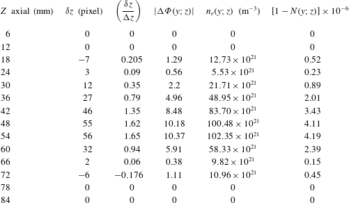
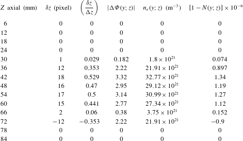
represented by the plots shown in figure 10 and tables 2–6 are computed using (2.22) and (2.24). In the above computations, we have taken the wavelength as
 ${\it\lambda}=600~\text{nm}$
and
 $L=10{\rm\pi}=60~\text{mm}$
, the diameter of the phase image to represent the plasma length along the
 $z$
axis. The inter-fringe spacing
 ${\rm\Delta}z=34~\text{pixels}$
. The refractive index of the plasma is always less than 1.
3. Results and discussion
The argon plasma image photographed in the laboratory by a CCD camera is obtained using the DC glow discharge technique (Saudy Reference Saudy2009). The argon plasma image used in the processing is shown in figure 1. It has dimensions of
 $512~\text{pixels}\times 512~\text{pixels}$
. The contour image of the argon plasma is plotted in figure 2. The interference shift of the argon plasma image using two-beam interference is obtained as shown in figure 3. Five horizontal discontinuous lines at 130, 180, 230, 280, and 330 pixels are represented in the same figure in order to compute the plasma fringe shifts.
The shifted central image is located inside a circle of diameter equal to
 $10{\rm\pi}=(512\times 6/8.6)$
as compared with the total image of
 $15{\rm\pi}=512~\text{pixels}$
. The phase image of argon plasma is computed from (2.10) using Matlab code. It is shown in figure 4. All images in figures 1–4 have dimensions of
 $512~\text{pixels}\times 512~\text{pixels}$
.
Two profiles at horizontal section, at 230 pixel, one for the uniform two-beam interference while the second is for the plasma-shifted interference, are plotted in figure 5.
Contour of the plasma image in the whole image of dimensions
 $512~\text{pixels}\times 512~\text{pixels}$
.

Interferometry shift of argon plasma image using two-beam interference. The image has dimensions of
 $512~\text{pixels}\times 512~\text{pixels}$
, and the shifted image is located in a circle of diameter equal to
 $10{\rm\pi}=(512\times 6/8.6)$
as compared with the total image of
 $15{\rm\pi}=512~\text{pixel}$
. Five horizontal discontinuous lines are shown at 130, 180, 230, 280, and 330 pixels to compute plasma fringe shifts represented in figure 10.

The phase image of argon plasma calculated directly using the arc tan function (2.10).

Two profiles taken at horizontal section at 230 pixel, one for the uniform two-beam interference while the second is for the plasma-shifted interference.

The axial shift occurring in the fringe system of two-beam interference, where the wavelength of illumination of the interferometer is
 ${\it\lambda}=600~\text{nm}$
, and the distance between two successive fringes
 ${\rm\Delta}z=12~\text{mm}$
in the image of total dimensions
 $512~\text{pixels}\times 512~\text{pixels}$
corresponding to dimensions of
 $11.5~\text{cm}\times 17.2~\text{cm}$
at magnification of
 $M=1.8$
. Fourteen fringes are shown as in figure 6(c).

Equation (2.3), which describes the intensity distribution of the multiple-beam interference, is used to draw the intensity map of the argon plasma superimposed over the interference pattern. Images at different frequencies of the interference pattern are plotted in figure 6(a–d). In case of multiple-beam interference a sharper fringe shift is obtained as compared with two-beam interference. This is useful to get an accurate measurement of the fringe shift in case of multiple-beam interference as compared with the two-beam interference fringe shift.
(a) Multiple-beam interference, where
 $F(x,y)=\text{sin}^{2}(2\ast y-{\it\psi}(x,y))$
. Twenty-nine fringes are shown as background fringes. (b) Multiple-beam interference, where
 $F(x,y)=\text{sin}^{2}(3\ast y/2-{\it\psi}(x,y))$
. Twenty-two fringes are shown as background fringes. (c) Multiple-beam interference, where
 $F(x,y)=\text{sin}^{2}(y-{\it\psi}(x,y))$
. Fourteen fringes are shown as background fringes. (d) Multiple-beam interference, where
 $F=\text{sin}^{2}(y/2-{\it\psi}(x,y))$
. Seven fringes are shown as background fringes.

Two profiles taken at horizontal section at 230 pixel, one for the uniform multiple-beam interference while the second is for the plasma-shifted interference.

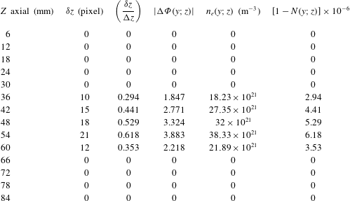
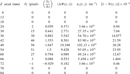
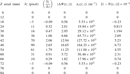
Computed values of the plasma phase shift
 ${\rm\Delta}{\it\phi}(y;z)$
, the plasma electron density
 $n_{e}(y;z)$
, and its refractive index
 $N(y;z)$
from the fringe shift at 130 pixel.

Two profiles at horizontal section 230 pixel, one for the background multiple-beam fringe system while the second is for the plasma-shifted interference, are plotted in figure 7.
The autocorrelation of the argon plasma image of dimensions
 $512~\text{pixels}\times 512~\text{pixels}$
is shown in figure 8. The profiles of the autocorrelation of the argon image at different horizontal sections is shown in figure 9. Eight plots are shown from the highest at 256 pixel followed by 200, 170, 150, 130, 100, 80, and 50 pixels.
Autocorrelation of the argon plasma image of dimensions
 $512~\text{pixels}\times 512~\text{pixels}$
.

Profiles of the autocorrelation of the argon image at horizontal sections. Eight plots are shown from the highest at 256 pixel followed by 200, 170, 150, 130, 100, 80, and 50 pixel.

The relation between the distance along the
 $z$
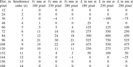
axis in mm and the axial shift of the image in nm is computed from (2.4), using table 1. As shown in figure 9, the highest fringe shift is located at the horizontal line at 230 pixel while the other two fringe shifts are located at horizontal lines 180 and 280 pixels. In the figure, the continuous line is drawn at 180 pixel while the discontinuous line is at 280 pixel.
Computed values of the plasma phase shift
 ${\rm\Delta}{\it\phi}(y;z)$
, the plasma electron density
 $n_{e}(y;z)$
, and its refractive index
 $N(y;z)$
from the fringe shift at 180 pixel.

Computed values of the plasma phase shift
 ${\rm\Delta}{\it\phi}(y;z)$
, the plasma electron density
 $n_{e}(y;z)$
, and its refractive index
 $N(y;z)$
from the fringe shift at 230 pixel.

Computed values of the plasma phase shift
 ${\rm\Delta}{\it\phi}(y;z)$
, the plasma electron density
 $n_{e}(y;z)$
, and its refractive index
 $N(y;z)$
from the fringe shift at 280 pixel.

Computed values of the plasma phase shift
 ${\rm\Delta}{\it\phi}(y;z)$
, the plasma electron density
 $n_{e}(y;z)$
, and its refractive index
 $N(y;z)$
from the fringe shift at 330 pixel.

The relation between the distance along the
 $z$
axis in pixels and the axial shift of the image in nm computed from (2.4) using two-beam interference is shown in figure 10. Five curves are plotted where the highest fringe shift is located at the line 230 pixel. Two other plots show a moderate shift for the red and blue curves at 180 and 280 pixels. The lowest two curves for shift are for 130 and 330 pixels. From the curves it is shown that the highest fringe shift is located near the plasma electrodes for the line 230 pixel while on moving farther from the electrodes the fringe shift decreases in proportion to its intensity. Hence, a plasma fringe mapping is obtained from the above results.
Five curves are plotted in the figure between the differential fringe shift
 ${\it\delta}z/{\rm\Delta}z$
and the distance along the axial plasma length in mm. The highest fringe shift is located at 230 pixel for the red curve. Two plots show a moderate shift at 180 and 280 pixels. The lowest two curves for shift are for 130 and 330 pixels.

4. Conclusion
We have extracted phase information of a plasma image using two-beam interference. A formula giving the phase shift of the image was derived. Also, a relation between the fringe shift and the plasma electron density was obtained. Consequently, the plasma refractive index was computed from the derived electron density. The multiple-beam interference images for the plasma shift showed higher contrast as compared with the images obtained in case of two-beam interference. Hence, accurate measurement of the fringe shift is attained.
Finally, the autocorrelation image of the argon plasma image and the corresponding profiles at different sections were made. All interference images for plasma, the contour, and correlation images were fabricated using Matlab code.