





1. Introduction
Economics studies the allocation of scarce resources among competing claims. In many applications, the focus is on the distribution of a budget over multiple items—a basket of goods purchased on a market, in individual choice problems, a multi-unit auction or multiple simultaneous contests, in strategic situations.
In lab experiments, to avoid confusing participants with too complex a task, the number of items under consideration is typically limited to a small number. For example, in their (Reference Dechenaux, Kovenock and Sheremeta2015) survey of experiments on different models of contests, Decheneaux et al. cite a total of 201 lab studies. Most study a single contest, but even when the focus is on multiple simultaneous contests, the number of contests is typically three or four, only rarely six or eight.Footnote 1 Some influential applications of these models, however, concern problems with large numbers of contested items. A classic example is Myerson (Reference Myerson1993): candidates compete to win an election, each has a budget to distribute freely over a continuum of voters, and each voter votes for the candidate who offers the most generous transfer. Myerson’s article is a fundamental contribution to voting theory, arguing that politically induced inequality among ex ante identical voters may be the natural result of democratic elections. It is also a very difficult theory to test in the field. And yet, it has never been tested in a lab, and neither have equally influential follow-up works that share the focus on politicians competing over voters or electoral districts (Dekel et al., Reference Dekel, Jackson and Wolinsky2008; Lizzeri and Persico, Reference Lizzeri and Persico2001; Lizzeri and Persico, Reference Lizzeri and Persico2005; Sahuguet and Persico, Reference Sahuguet and Persico2006; Snyder, Reference Snyder1989). The difficulty is in designing an experiment that asks participants to allocate resources over a very large number of items, and still keeps the task transparent enough for them to think rationally over the possible choices.
The purpose of this note is to propose an experimental interface that addresses this challenge. The interface is driven by two main ideas. First, in contrast to asking participants for their allocations item by item, as is typically done, participants are asked to draw a curve over a stylized representation of the many items. The curve can be modified freely, with the budget constraint automatically enforced by the computer. Second, the curve depicts relative levels of resources over the multiple items, rather than absolute levels. When a participant adjusts the curve, for example by increasing resources on one of the items, the budget is automatically rebalanced so as to satisfy the constraint while maintaining all other relative values constant. As a result, the curve remains visually stable. If the curve showed absolute levels, satisfying the budget constraint would require the whole curve to shift in response to any change, creating a very difficult environment for the subjects.
To our knowledge, the existing experimental interface closest to our goals is the Distribution Builder (Goldstein et al., Reference Goldstein, Johnson and Sharpe2008; Sharpe et al., Reference Sharpe, Goldstein and Blythe2000), an interactive tool used to elicit respondents’ preferences over investment portfolios.Footnote 2 The Distribution Builder asks subjects to provide a desired distribution of probabilities over future wealth under a cost constraint. The interface computes the least costly portfolio that generates the desired distribution given the prices of available assets, and each subject modifies (by “tatonnement”) the desired distribution to meet the cost constraint.
Besides the graphical appearance, our interface and the Distribution Builder have other differences. First, our curve is not a probability distribution; it is a direct allocation of resources. Second, we ask subjects to draw a continuous curve indicating relative levels of expenditure across item values. Thus we call attention to the curve’s shape and slope, as opposed to the vector of absolute expenditures, item by item. Third, we implement the budget constraint very differently. In our case, subjects are allowed to draw any curve at all, and the budget constraint is imposed ex post by the computer, when translating relative allocations into absolute levels of expenditure. The Distribution Builder, on the other hand, prevents subjects from finalizing the distribution unless the budget constraint is met. Because asset prices are an important component of the exercise and are not described to the subjects, experimenting with the budget constraints allows subjects to learn them. In our case, there are no hidden prices, and the budget is a straightforward sum of allocated resources.
Because we are not familiar with other experimental interfaces asking participants to express their allocations by drawing a curve and because the range of problems to which the approach could be applied is large, we hope that a detailed description of the interface may be useful to others. The platform was constructed by Destinybit (https://destinybit.com/), a game design company. We describe in the Supplementary Material how to download the program and how to parametrize it for the specific game we studied. However, the logic behind the platform’s design is more flexible than the particular application and can be reproduced in different programs. It is such logic, more than the software itself, that is the purpose of this note.
2. The experimental interface
The interface was built for the experiment discussed in Casella et al. (Reference Casella, Compte and Si2024). For the sake of concreteness, we briefly describe the game here. We study a Blotto game where two opponents are each endowed with a budget of resources  $R_{i}$, to be distributed over a continuum of battlefields. The battlefields have different values
 $v\in\mathcal{V}$, drawn independently from a common distribution
 $f(v)$. Independence holds both across battlefields, for given player, and across the two opponents, for given battlefield. Each battlefield is won by the player who allocates to it more resources. A player’s strategy is a resource allocation function
 $b_{i}(v)$ that maps the battlefields’ values into resources allocated to each value, under the constraint that the resource constraint be satisfied, or
 $\int_{\mathcal{V}}b_{i}(v)f(v)dv=R_{i}$. The object of interest is the allocation function
 $b_{i}(v)$. The theory delivers specific predictions on the shape of such function in equilibrium; the challenge was eliciting such a function experimentally.Footnote 3
In the experiment, we framed the battlefields as assets to be defended and represented them as marbles of different values. All marbles a player owns eventually clash with another player’s marbles in one-to-one duels, but before duels occur, players make their marbles “stronger” by endowing them with defenses from a known budget of defenses. In each duel, the marble with lower defenses is destroyed, the stronger one survives, and its owner earns the marble’s value as points. As mentioned, the Appendix provides a link for downloading the program, as well as instructions on how to make some modifications to the original game, for example by changing the distribution  $f(v)$, or allowing for asymmetric budgets
 $R(i)$, or introducing correlation in values.
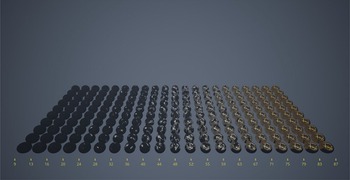
At the start of the experiment, each participant sees the marbles with which each is endowed. These are the assets, of different values, the participant will have to defend. With  $f(v)$ Uniform, the first screen corresponds to Figure 1.
Experimental interface: opening screen.  $f(v)$ uniform; 210 marbles

To approximate the continuous distribution, players must be endowed with as many marbles as possible. But when the number is large, handling each marble separately (appreciating its value and choosing the desired level of defenses) is infeasible. Marbles must then be organized in classes. In practice, players are faced with 21 classes of marbles, organized in columns, with each column corresponding to a different value, and all marbles in the same column having the same value. Thus the marbles can take any of 21 different values, roughly suggested by their color, from black to gold, and reported more precisely by the number at the bottom of each column. In the case of a Uniform distribution, as in the example of Figure 1, all columns have the same number of marbles (here, 10), and thus there is a total of 210 marbles. All marbles will fight duels.Footnote 4
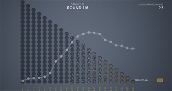
A player’s task is the allocation of defenses to the player’s marbles. Defenses are not represented through objects but graphically, through a curve each player draws, the literal experimental counterpart of the  $b(v)$ bidding function of the theoretical model. We asked each participant to allocate defenses by moving the cursor of the computer mouse smoothly over the image of the marbles. All marbles in the same column receive the same amount of defenses, represented by the height of the curve over that column. Figure 2 is an example we used in the instructions for the case of a triangular distribution
 $f(v)$.
Experimental interface: distribution of defenses. Example with  $f(v)$ triangular; 231 marbles

Figure 2 Long description
A line graph displays defense allocation across marble columns in a triangular distribution setup. The x-axis represents marble columns, with values labeled at 6, 11, 11, 11, 14, 20, 41, 51, 63, 77, 87, 90, 94, 94, 90, 80, 77, 71, 69, 66, and 64. A second row of values beneath these reads 0, 6, 13, 19, 26, 32, 39, 45, 52, 58, 65, 71, 78, 84, 91, 97, 104, 110, 117, 123, and 130. The y-axis represents the height of the defense curve over each column, with no numeric scale labeled. The curve starts at a low level at column 6, remains relatively flat through columns 11 to 20, then rises steadily through columns 41 to 63, reaching a visible peak in the region of columns 90 to 94. After this peak, the curve declines gradually as column number increases further, ending at a lower level near column 64 at the far end of the x-axis range. The marbles in each column are stacked vertically, and the height of the curve above each column represents the amount of defense allocated to that column.
Although only 21 different values are thus relevant when allocating defenses, the game is much more intuitive if presented as if the value distribution were continuous. When asked to draw a curve, players focus on the shape of the curve, that is, on the slope of the allocation function—the change in defenses as the values of the marbles increase—as opposed to choosing the exact numerical amount of defenses assigned to each of the 21 values. This short video gives an idea of the interface. We describe the different steps in the next section.
3. Eliciting the defense allocation function
Asking participants to draw a curve creates two related challenges. First, the visualization of different allocations needs to be somewhat robust to the scale of the graph: the image on the screen must remain legible whether the player devotes all defenses to a single column, or divides them less asymmetrically. We set  $R_{i}=10,000$ to allow for a fine enough variation in assigned defenses while still expressing them in integer numbers. As a result, however, the absolute value of defenses assigned to each marble could vary widely, creating difficulties with the visualization. In the Uniform case, for example, with
 $R_{i}=10,000$, the amount of defenses assigned to a marble could vary between 0 and 1,000 (taking into account that all marbles in the same column must receive the same defenses). But then the difference between, say, 25 and 50, would be impossible to see, even though one number is twice the other. Second, the defense budget must be satisfied. If we asked participants to draw absolute resource allocations, then revising the defenses assigned to one column would force other allocations to change as well, to enforce the budget constraint. The global change in the curve would be sure to generate confusion. Asking participants to report graphically the relative allocation of defenses per column addresses both problems.Footnote 5
Call 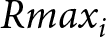 $Rmax_{i}$ the maximal defense assigned by player
 $i$ to any marble (note: any marble, not any column, since, depending on the distribution
 $f(v)$, columns can have different numbers of marbles, as they do in Figure 2).
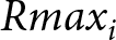 $Rmax_{i}$ provides the anchor against which relative allocations are calculated. Its value, in absolute terms, is calculated by the computer for any allocation of reserves, so as to satisfy the budget constraint, and adjusts with any change to the allocation.
The vertical axis corresponds to fractions of 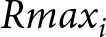 $Rmax_{i}$ and ranges between 0 and
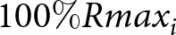 $100\% Rmax_{i}$. In Figure 2, the curve is three times higher in column 7 relative to columns 2, 3 and 4, and thus the curve assigns three times as many defenses to any marble in column 7, relative to any marble in columns 2, 3, and 4. The larger number at the foot of each column indicates the absolute defenses assigned to each marble in the column, while the smaller number reminds the player of the value of the marbles in the column.
At the start, before actively allocating defenses, the subjects see a horizontal line over all columns, an initial allocation curve assigning equal defenses to all marbles.Footnote 6 During play, participants modify the curve. Participants modify a point on the curve by clicking on it and raising or lowering it.
The curve is anchored by points we call anchors. A point on the curve becomes an anchor by being clicked on, giving the visual impression of “grabbing” the curve at that point. Only points corresponding to a column can be anchors, but because the columns fill compactly the whole screen, the player’s perception is that any point on the curve can be clicked on and modified. In addition, although each individual point can only be moved vertically, the density of columns on the screen means that when drawing a continuous curve the experience approximates closely the sense of drawing without constraints.Footnote 7 In practice, as a participant draws a curve by moving the cursor of the mouse freely over the marbles, the points corresponding to all columns typically become anchors.
Anchors matter because when participants raise or lower one point, the curve only changes between the two closest anchors, on the point’s either side: the segments of the curve between the point and its closest anchors on the point’s two sides adjust by linear interpolation. The other segments, outside the two closest anchors, do not move. When, as most likely, points corresponding to all columns have become anchors, modifying the curve over one column has no effect on the height of the curve over any other column. To reiterate our main point, this is possible because the curve represents relative defenses. If it represented absolute defenses, the entire curve would move in response to any revision because all allocations of absolute defenses (including 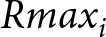 $Rmax_i$) would have to change to satisfy the budget constraint.
To calculate the amount of absolute defenses assigned to any column, the program solves two problems. First, the program determines the defenses assigned to each marble, expressed in percentage of 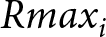 $Rmax_{i}$, by linear interpolation between any two anchors. Second, the program calculates
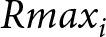 $Rmax_i$.
The first step corresponds to the visual changes of the curve, as the player makes any adjustments. For example, if the vertical height of the allocation curve is set at 20 at position (value) 75, and at 100 at position 100, if both are anchors, and there is no other anchor between them, then at position 80 the allocation curve is set automatically at  $20+[(100-20)/(100-75)] \times 5=36$. If we call
 $x$ the horizontal position (recall that
 $x$ is the value of marbles at the corresponding column) and
 $y$ the height, then:
 \begin{equation*}
y_{m} = y_{l}+\left(\frac{y_{r}-y_{l}}{x_{r}-x_{l}}\right)(x_{m}-x_{l})
\end{equation*}
where  $m$ denotes the point of interest, intermediate relative to the anchors to the left (
 $l$) and to the right (
 $r$). Here
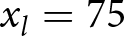 $x_{l}=75$,
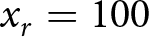 $x_{r}=100$,
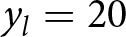 $y_{l}=20$,
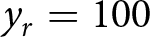 $y_{r}=100$, and
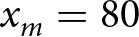 $x_{m}=80$. Hence
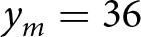 $y_{m}=36$.
If the subject decides to move the curve at position 80, then the height at position 80 is determined by the subject, while the heights strictly between position 75 and position 100 (the two closest anchors on the two sides) are determined by the equation above. If 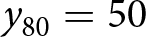 $y_{80}=50$, for example, then:
 \begin{equation*}
\begin{aligned}
y & = 20 +\left(\frac{50-20}{80-75}\right)(x-75) \text{for all points between positions 75 and 80}\\
y & = 50 +\left(\frac{100-50}{100-80}\right)(x-80) \text{for all points between positions 80 and 100.}
\end{aligned}
\end{equation*}
The curve does not change at or below position 75. This is the program’s first step.
As a second step, given the defenses assigned to each marble as proportion of 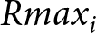 $Rmax_{i}$, the program calculates
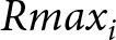 $Rmax_{i}$ using the constraint that all defenses must equal the total budget. Given the value of
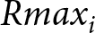 $Rmax_{i}$, the program then translates all relative defenses into absolute values, reported numerically at the bottom of each column.
If we call  $n_{c}$ the number of marbles in column
 $c$,
 $C$ the total number of columns (21 in our implementations), and
 $y_{c}$ the height of the curve at column
 $c$, then
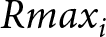 $Rmax_{i}$ must solve:
 \begin{equation*}
\sum_{c=1}^{C}n_{c}\frac{y_{c}}{100}Rmax_{i}=R_{i}
\end{equation*}
where  $R_{i}$ is
 $i$’s total available defense budget.
In the example of Figure 2, the total number of marbles is 231, divided in 21 columns with  $\{21,20,...,1\}$ marbles each. At the opening screen,
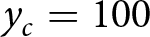 $y_{c}=100$ for all columns; if
 $R_{i}=10,000$, we have
 $231(100/100)Rmax_{i}=10,000$, or, rounding up,
 $Rmax_{i}=43$. Since at the opening screen
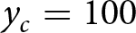 $y_{c}=100$ (or 100%
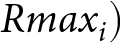 $Rmax_{i})$, every marble is allocated absolute defenses equal to 43. Suppose instead, for example,
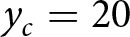 $y_{c}=20$ for the first 10 columns, and 100 for columns 11-21. Then:
 $\left(\sum_{z=12}^{21}z(20/100)+\sum_{z=1}^{11}z(100/100)\right)Rmax_{i}=10,000$, or, after rounding,
 $Rmax_{i}=101$. Each marble in the first 10 columns is allocated defenses just above 20, and each marble in columns 11-21 defenses equal to 101.
As the player manipulates the curve, all larger numbers at the foot of each column, representing the absolute amount of defenses assigned to each marble in the column, necessarily change (to respect the budget constraint), while the curve remains stable beyond the two anchors closest to the point the player has modified. The program stores, for each player, the vector of 21  ${x,y}$ values along the final allocation curve, as well as the history of revisions made by the player.
The computer interface was designed to maximize the sense of drawing a continuous curve and little practice is sufficient to generate the allocation curve by moving the mouse smoothly over the profile of all marbles. The curve can be manipulated easily—for example, players can delete a point by right-clicking on it (and the height of the allocation curve at that point is then interpolated linearly from the two nearest anchors)Footnote 8—and at any modification the constraint that the entire defense budget be allocated is imposed automatically by the computer. The design allows players to draw a defense allocation function that is intuitive, uses the full budget, and remains stable as details are fine-tuned.
Supplementary material
The supplementary material for this article can be found at https://doi.org/10.1017/esa.2026.10035.
Funding
We thank Gian Paolo Vernocchi and Simone Daminato at Destinybit for their programming expertise and creativity, Jean Francois Laslier for inspiring conversations on the initial design, and the Institute for Social and Economic Research and Policy (ISERP) at Columbia University for financial support.






 Open access

