2.1 Multi-agent RL

In MARL, multiple RL agents are deployed into a common environment. The single-agent Markov decision process (MDP) framework becomes inadequate when multiple autonomous agents act simultaneously in the same domain. Instead, the more general stochastic game (SG) may be used in the case of a MAS (Buşoniu et al., Reference Buşoniu, Babuška and Schutter2010). A SG is defined as a tuple <S, A _1...N , T, R _1...N >, where N is the number of agents, S is the set of system states, A _i is the set of actions for agent i (and A is the joint action set), T is the transition function, and R _i is the reward function for agent i.

The SG looks very similar to the MDP framework, apart from the addition of multiple agents. In fact, for the case of N=1 a SG then becomes a MDP. The next system state and the rewards received by each agent depend on the joint action a of all of the agents in a SG, where a is derived from the combination of the individual actions a _i for each agent in the system. Each agent may have its own local state perception s _i , which is different to the system state s (i.e. individual agents are not assumed to have full observability of the system).

Note also that each agent may receive a different reward for the same system state transition, as each agent has its own separate reward function R _i . In a SG, the agents may all have the same goal (collaborative SG), totally opposing goals (competitive SG), or there may be elements of collaboration and competition between agents (mixed SG). Whether RL agents in a MAS will learn to act together or at cross-purposes depends on the reward scheme used for a specific application.

At each timestep in a SG, agents sense their own local state information s _i and each agent chooses an action a _i ∈A _i according to the policy π _i ∈Π _i that it is currently following. The product of all the individual actions results in a system joint action a∈A, and the joint action a selected in a system state s determines the next system state s′. All agents in the SG are then rewarded for this transition between system states based on the return from their individual reward functions R _i .

Model-free learners sample the underlying MDP or SG directly in order to gain knowledge about the unknown model, in the form of value function estimates (Q values). These estimates represent the expected reward for each state action pair, which aid an agent in deciding which action is most desirable to select when in a certain state. An agent must strike a balance between exploiting known good actions and exploring the consequences of new actions in order to maximize the reward received during its lifetime. Two strategies that are commonly used to manage the exploration exploitation trade-off are ε-greedy and softmax (Wiering & van Otterlo, Reference Wiering and van Otterlo2012). Q-learning (Watkins, Reference Watkins1989) is one of the most commonly used model-free RL algorithms. In Q-learning, the Q values are updated according to Equation (1), where α∈[0, 1] is the learning rate and γ∈[0, 1] is the discount factor.

(1) $$Q(s,a)\leftarrowQ(s,a){\plus}\alpha [r{\plus}\gamma \mathop {\max }\limits_{a'} Q(s',a'){\minus}Q(s,a)]$$

One of two different approaches is typically used when RL is applied to MAS: multiple individual learners or joint action learners. In the former case multiple agents are deployed into a common environment, each using a single-agent RL algorithm (e.g. Q-learning), whereas joint action learners use multi-agent specific algorithms which take account of the presence of other agents. A significant drawback inherent in the joint action learners approach is the exponential increase in the size of the state-action space for each additional agent that is added to a system (Claus & Boutilier, Reference Claus and Boutilier1998). For this reason multiple individual learners are considered in this work.

When multiple self-interested agents learn and act together in the same environment, it is generally not possible for all agents to receive the maximum possible reward. Therefore, MAS are typically designed to converge to a Nash equilibrium (Shoham et al., Reference Shoham, Powers and Grenager2007). This notion of equilibrium was first introduced by (Nash, Reference Nash1951), and is one of the most important concepts used to analyze MAS (Wooldridge, Reference Wooldridge2001).

Formally, a joint policy π ^NE leads to a Nash equilibrium when:

(2) $$\matrix{ {\forall i\in\{ 1,...,N\} ,\pi _{i} \in\Pi _{i} \,\mid\,R_{i} (\pi _{i}^{{NE}} {\cup}\pi _{{{\minus}i}}^{{NE}} )\geq R_{i} (\pi _{i} {\cup}\pi _{{{\minus}i}}^{{NE}} )} \hfill \cr } $$

where Π is the set of joint policies, Π_−i is the set of joint policies excluding the set of policies Π _i for agent i, and $$\pi _{i}^{{NE}} $$ is a specific policy followed by agent i when all other agents follow their policies from $$\pi _{{{\minus}i}}^{{NE}} $$ .

Whenever the above inequality holds true for all possible policies for all agents in a MAS, a Nash equilibrium exists. In other words, a Nash equilibrium occurs whenever any individual agent cannot improve its own utility by changing its behaviour, assuming that all other agents in the MAS continue to behave in the same way.

In cooperative MAS, coordinating agents’ actions to achieve the highest possible system utility is a difficult problem. While it is possible for multiple individual Q-learners in a cooperative MAS to converge to a point of equilibrium, there is no theoretical guarantee that the agents will converge to an optimal joint policy (one which maximizes the system utility).

2.2 Credit assignment in MAS

As RL agents seek to maximize the rewards that they receive, the design of the reward function directly affects the joint policies learned, and thus the issue of credit assignment in MARL is an area of active research. Two typical reward functions for MARL exist: local rewards unique to each agent and global rewards representative of the group’s performance (Devlin et al., Reference Devlin, Yliniemi, Kudenko and Tumer2014).

A local reward (L _i ) is based on the utility of the part of a system that agent i can observe directly. Individual agents are self-interested, and each will selfishly seek to maximize its own local reward signal, often at the expense of global system performance when locally beneficial actions are in conflict with the optimal joint policy.

A global reward (G) provides a signal to the agents which is based on the utility of the entire system. Rewards of this form encourage all agents to act in the system’s interest, with the caveat that an individual agent’s contribution to the system performance is not clearly defined. All agents receive the same reward signal, regardless of whether their actions actually improved the system performance, resulting in a low ‘signal to noise ratio’ (Agogino & Tumer, Reference Agogino and Tumer2008).

RL agents typically learn how to act in their environment guided by the reward signal alone. Reward shaping provides a mechanism to guide an agent’s exploration of its environment, via the addition of a shaping signal to the reward signal naturally received from the environment. The goal of this approach is to increase learning speed and/or improve the final policy learned.

Generally, the reward function is modified by the addition of a shaping reward, as shown in Equation (3) below:

(3) $$R'{\equals}R{\plus}F$$

where R is the original reward function, F is the additional shaping reward and R′ is the modified reward signal given to the agent. Empirical evidence has shown that reward shaping can be a powerful tool to improve the performance of RL agents; however, it can modify the original goal(s) of the problem if it is not applied carefully (Randløv & Alstrøm, Reference Randløv and Alstrøm1998).

PBRS was proposed to deal with such problems. When implementing PBRS, each possible system state has a certain potential, which allows the system designer to express a preference for an agent to reach certain system states. (Ng et al., Reference Ng, Harada and Russell1999) defined the additional shaping reward F for an agent receiving PBRS as shown in Equation (4) below:

(4) $$F(s,s'){\equals}\gamma \Phi (s'){\minus}\Phi (s)$$

where Φ(s) is a potential function which returns the potential for a state s, and γ is the same discount factor used when updating value function estimates. PBRS has been proven not to alter the optimal policy of a single agent acting in an MDP (Ng et al., Reference Ng, Harada and Russell1999) , or the set of Nash equilibria in the case of multiple agents acting in a SG (Devlin & Kudenko, Reference Devlin and Kudenko2011). Furthermore, Devlin and Kudenko (Reference Devlin and Kudenko2012) also proved that the potential function can be changed dynamically during learning, while still preserving the guarantees of policy invariance and consistent Nash equilibria. Recent analysis by Grześ (Reference Grześ2017) has shown that the potential of the terminal state must be zero to preserve theoretical guarantees in finite horizon domains. PBRS does not alter the set of Nash equilibria of a MAS, but it can affect the joint policy learned. It has been empirically demonstrated that groups of agents guided by a well-designed potential function can learn at an increased rate and converge to better joint policies, when compared to agents learning without PBRS (Devlin et al., Reference Devlin, Grzes and Kudenko2011a; Devlin et al., Reference Devlin, Yliniemi, Kudenko and Tumer2014; Mannion et al., Reference Mannion, Devlin, Duggan and Howley2017). However, with an unsuitable potential function, groups of agents learning with PBRS can converge to worse joint policies than those learning without PBRS.

A difference reward (D _i ) is a shaped reward signal that aims to quantify each agent’s individual contribution to the system performance in a cooperative MAS (Wolpert et al., Reference Wolpert, Wheeler and Tumer2000). Formally:

(5) $$D_{i} (s_{i} ,a_{i} ){\equals}G(s,a){\minus}G(s_{{{\minus}i}} {\cup}s_{i}^{c} ,a_{{{\minus}i}} {\cup}a_{i}^{c} )$$

where G (s, a) is the global system utility, s is the system state, a is the joint action, and $$G(s_{{{\minus}i}} {\cup}s_{i}^{c} ,a_{{{\minus}i}} {\cup}a_{i}^{c} )$$ is the counterfactual which represents the global utility for a theoretical system without the contribution of agent i. The terms s _−i and a _−i refer to all the states and actions not involving agent i, while $$s_{i}^{c} $$ and $$a_{i}^{c} $$ are fixed states and actions not dependent on agent i. Typically, the counterfactual system utility is calculated with agent i removed, or by assuming a default state/action for agent i. Difference rewards are a well-established shaping methodology, with many successful applications in MARL (see e.g. Wolpert & Tumer, Reference Wolpert and Tumer2002; Tumer & Agogino, Reference Tumer and Agogino2007; Mannion et al., Reference Mannion, Devlin, Duggan and Howley2016; Mannion et al., 2016Reference Mannion, Duggan and Howleyb ). Recent work has extended D to increase its effectiveness in problem domains where agents’ actions must be tightly coordinated to achieve a high level of system performance (Rahmattalabi et al., Reference Rahmattalabi, Chung, Colby and Tumer2016).

2.3 Multi-objective RL

Single-objective optimization approaches seek to find a single solution to a problem, whereas in reality a system may have multiple conflicting objectives that could be optimized. Multi-objective optimization (MOO) approaches on the other hand address the requirement to make a trade-off between competing objectives. Compromises between competing objectives can be defined using the concept of Pareto dominance (Pareto, Reference Pareto1906). The Pareto optimal set or NDS consists of solutions which are incomparable, where each solution in the set is not dominated by any of the others on every objective. In MORL the reward signal is a vector, where each component represents the performance on a different objective.

The hypervolume metric measures the spread of a given set of non-dominated solutions; therefore, the diversity and accuracy of any set of solutions produced by an algorithm can easily be evaluated, by comparing its hypervolume with that of the NDS produced by a competing algorithm, or with that of the true Pareto front of the application domain (if known).

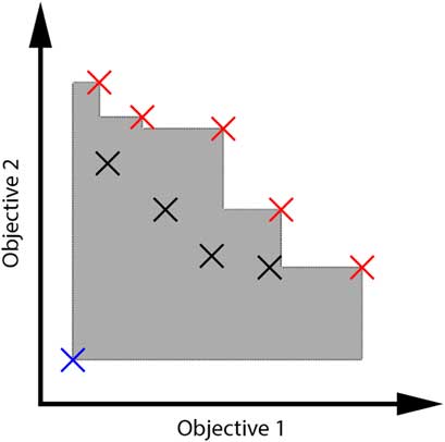
In domains where the true Pareto front is known, its hypervolume represents an absolute maximum level of performance that may be achieved by an agent (or by a group of agents in the case of a cooperative MAS). Figure 1 illustrates the process of determining which solutions constitute a NDS in a bi-objective maximization problem, and of calculating its hypervolume with respect to a given reference point.

Figure 1

Solutions in red form the non-dominated set (NDS), while solutions in black are said to be dominated. The shaded area denotes the hypervolume of the NDS with respect to the reference point (shown in blue).

MORL problems may be defined using the MDP or SG framework as appropriate, in a similar manner to single-objective problems. The main difference lies in the definition of the reward function: instead of returning a single scalar value r, the reward function R in multi-objective domains returns a vector r consisting of the rewards for each individual objective c∈C. Therefore, a regular MDP or SG can be extended to a multi-objective MDP (MOMDP) or MOSG by modifying the return of the reward function.

It follows that the value function V ^π (s) in multi-objective domains returns a vector v whose components are the expected discounted returns for each objective when starting in state s and following a policy π (Roijers et al., Reference Roijers, Vamplew, Whiteson and Dazeley2013):

(6) $${\bf V}^{\pi } (s){\equals}E^{\pi } \{ \mathop{\sum}\limits_{k{\equals}0}^\infty \gamma ^{k} {\bf r}_{{t{\plus}k{\plus}1}} \,\mid\,s_{t} {\equals}s\} $$

A policy π ^*∈Π (where Π is the set of possible policies) is Pareto optimal if for every π∈Π either,

(7) $$\forall _{{c\in C}} [{\bf V}_{c}^{\pi } (s_{0} ){\equals}{\bf V}_{c}^{{\pi ^{{\asterisk}} }} (s_{0} )]$$

or, there is at least one c∈C such that

(8) $${\bf V}_{c}^{\pi } (s_{0} )\,\lt\,{\bf V}_{c}^{{\pi ^{{\asterisk}} }} (s_{0} )$$

where $${\bf V}_{c}^{\pi } (s_{0} )$$ is the expected discounted return for objective c when starting in state s ₀ and following the policy π. That is, π* is Pareto optimal if there exists no feasible policy π which would increase the value of one objective beyond that of π* without causing a simultaneous decrease in the value of another objective. A policy that does not meet these criteria is dominated by another policy in Π. All policies not dominated by another are part of the NDS.

The majority of MORL approaches make use of single-policy algorithms in order to learn Pareto optimal solutions. Examples of single-policy algorithms include traditional temporal difference methods such as Q-learning and SARSA. In order to apply single-policy algorithms to MORL problems, scalarization functions may be used to transform a reward vector r into a scalar reward signal r (Roijers et al., Reference Roijers, Vamplew, Whiteson and Dazeley2013). An agent learns using the scalarized version of the reward vector, and selects actions as normal by comparing the scalarized Q values for actions in a given state (using e.g. ε -greedy).

Linear scalarization is commonly used in MORL literature (see e.g. Vamplew et al., Reference Vamplew, Dazeley, Berry, Issabekov and Dekker2010; Roijers et al., Reference Roijers, Vamplew, Whiteson and Dazeley2013; Van Moffaert et al., Reference Van Moffaert, Drugan and Nowé2013; Brys et al., Reference Brys, Pham and Taylor2014; Mason et al., Reference Mason, Mannion, Duggan and Howley2016; Mannion et al., Reference Mannion, Mason, Devlin, Duggan and Howley2016c, Reference Mannion, Mason, Devlin, Duggan and Howley2016d; Yliniemi & Tumer, Reference Yliniemi and Tumer2016), and is defined in Equation (9) below:

(9) $$r_{{\plus}} {\equals}\mathop{\sum}\limits_{c\in C} {\bf w}_{c} {\bf r}_{c} $$

where w is the objective weight vector, w _c is the weight for objective c, r ₊ is the scalarized reward signal, r _c is the component of the reward vector r for objective c, and C is the set of objectives. When using linear scalarization, altering the weights in the weight vector allows the user to express the relative importance of the objectives.

Scalarized MORL approaches sometimes make use of normalization where the scale of the expected returns varies between objectives, or to simplify the process of selecting objective weights in the case of linear scalarization. The normalized score on objective c may be calculated as (Marler & Arora, Reference Marler and Arora2004):

(10) $${\bf r}_{c}^{{norm}} {\equals}{{{\bf r}_{c} {\minus}{\bf r}_{c}^{{min}} } \over {{\bf r}_{c}^{{max}} {\minus}{\bf r}_{c}^{{min}} }}$$

where $${\bf r}_{c}^{{norm}} $$ is the normalized score on objective c, and $${\bf r}_{c}^{{max}} $$ and $${\bf r}_{c}^{{min}} $$ are the utopia and nadir values for objective c.

MOO approaches typically seek to produce a set of solutions that approximate the true Pareto front of a problem. In order to produce a set of Pareto optimal solutions using scalarized single-policy RL algorithms, researchers typically record the best non-dominated solutions found during a number of independent runs (see e.g. Vamplew et al., Reference Vamplew, Dazeley, Berry, Issabekov and Dekker2010; Van Moffaert et al., Reference Van Moffaert, Drugan and Nowé2013; Yliniemi & Tumer, Reference Yliniemi and Tumer2016; Mannion et al., Reference Mannion, Devlin, Mason, Duggan and Howley2017). These solutions are then compared with one another to produce an approximation of the Pareto front.

For a more complete overview of MORL beyond the sumary presented in this section, the interested reader is referred to a survey article by Roijers et al. (Reference Roijers, Vamplew, Whiteson and Dazeley2013).

2.4 Multi-objective MAS

This section discusses related work that takes a multi-objective perspective on cooperative MAS, with a specific focus on the works that are most closely related to the contributions of this article.

Brys et al. (Reference Brys, Pham and Taylor2014) applied MORL to a traffic signal control problem, where each intersection in a 2×2 grid is controlled by an individual agent. Their work demonstrated that rewarding agents with a linear scalarized combination of delay and throughput improved delay times when compared to agents rewarded using delay alone. However, their approach uses local rewards (i.e. each agent is rewarded based on conditions at its assigned intersection only), and does not make any attempt to encourage coordination between the agents.

Van Moffaert et al. (Reference Van Moffaert, Brys, Chandra, Esterle, Lewis and Nowé2014) tested MORL on a multi-objective multi-agent smart camera problem. They developed an adaptive weight algorithm (AWA) which is used to choose the weighting between the two system objectives when linear scalarization is applied. The AWA algorithm was found to improve learning speed, obtaining improved solutions in terms of hypervolume and a better spread in the objective space, when compared with other weight selection methods that were tested.

Taylor et al. (Reference Taylor, Dusparic, Galván-López, Clarke and Cahill2014) proposed parallel transfer learning (PTL) as a mechanism to accelerate learning, by sharing experience among agents. PTL was tested on a multi-objective multi-agent smart grid problem, and was found to improve learning speed and final performance when compared to agents learning without PTL.

Mason et al. (Reference Mason, Mannion, Duggan and Howley2016) applied MARL to a multi-objective water resource management problem, and found that it could produce solutions of similar quality to those produced by particle swarm optimization (PSO). In this work, the authors did not consider the effect of credit assignment; agents were rewarded using the unshaped system evaluation function only.

Roijers et al. (Reference Roijers, Whiteson and Oliehoek2013, Reference Roijers, Whiteson and Oliehoek2014, Reference Roijers, Whiteson and Oliehoek2015) consider the effect of encouraging coordination in their research on cooperative MOMAS. Their approach makes use of multi-objective coordination graphs (MO-CoGs) which model the interactions between agents. MO-CoGs are used to calculate joint actions that will cover the Pareto front, or a subset of the Pareto front. Multiple individual Q-learners with reward shaping are used throughout this article. By comparison with MO-CoGs, our approach does not require a model of the agents’ interactions to determine the Pareto optimal joint actions. Reward shaping instead assumes that some domain knowledge is available to encourage coordination and selection of Pareto optimal joint actions.

None of the works discussed thus far considered the effect of credit assignment in MOMAS. (Yliniemi & Tumer, Reference Yliniemi and Tumer2016) present the first work that considers the design of reward structures in a MOMARL setting. Their work compared the effectiveness of D with that of the typical MARL reward structures L and G. Experimental work conducted in a multi-objective congestion problem, and a multi-objective robot coordination problem confirmed that D can improve MOMARL performance when compared to L or G, both in terms of learning speed and the quality of the non-dominated solutions found. Yliniemi & Tumer, Reference Yliniemi and Tumer2016 also demonstrated that D can be used effectively with multi-objective GAs, in a series of experiments where it was applied to shape the fitness function of NSGA-II (non-dominated sorting genetic algorithm).

Mannion et al. (Reference Mannion, Devlin, Mason, Duggan and Howley2017) demonstrated that agents learning using PBRS along with a suitable potential function in MOSGs can outperform agents learning using unshaped G in terms of learning speed, average performance on system objectives, and quality of the non-dominated solutions found. It has been theoretically proven that applying PBRS in a MOMDP or MOSG does not alter the true Pareto optimal set of solutions (Mannion et al., Reference Mannion, Devlin, Mason, Duggan and Howley2017), although no corresponding guarantees are yet available for D. While applying PBRS does not alter the true Pareto front of a MOSG, it may alter the Nash equilibrium reached by the agents, and therefore different policies could be learned compared to agents learning without PBRS.

However, the set of possible policies that could be learned and their Pareto relation to one another remains consistent when PBRS is applied. As with single-objective SGs, PBRS affects the agents’ exploration, and therefore the quality of the heuristic information used determines how successful a particular PBRS application will be. In the case of D, the preexisting guarantees are weaker; it has been proven that the relative ordering of expected returns (and therefore the Nash equilibria) are not altered when agents are rewarded using D instead of G in two-player single-objective matrix games (Colby & Tumer, Reference Colby and Tumer2015).

None of the above works empirically evaluated the effect of applying D or PBRS in a MOSG where the true Pareto optimal solutions are known, or considered if it is possible in practice for agents to sample true Pareto optimal solutions under such reward transformations.

2.5 Contributions of this work

This article will consider the issue of credit assignment in MOMAS, where each agent is an individual Q-learner. Clearly, the most closely related works discussed in this section are those of Yliniemi and Tumer (Reference Yliniemi and Tumer2016) and Mannion et al. (Reference Mannion, Devlin, Mason, Duggan and Howley2017b). While these works have already separately demonstrated the importance of appropriate credit assignment and the effectiveness of D and PBRS in MOMARL, they lack:

• ∙ A theoretical evaluation of the effect of D in MOSGs. Specifically, the question of whether applying D to MOSGs will alter the true Pareto optimal joint policies remains open.

• ∙ Empirical evaluations of reward shaping in a MOSG where the true Pareto optimal system utilities are known.

• ∙ Empirical comparisons between D and PBRS in MOMARL domains.

This work addresses these gaps in the literature by presenting a theoretical analysis of the effects of difference rewards which justifies their use in MOSGs (Section 3), followed by empirical studies using D and PBRS in a domain where the true Pareto optimal solutions are known (Section 4), and in a realistic application domain (Section 5).

4.1 Multi-Objective Beach Problem Domain

The MOBPD extends an earlier single-objective version introduced by Devlin et al. (Reference Devlin, Yliniemi, Kudenko and Tumer2014), in a similar manner to the multi-objective extension (Yliniemi & Tumer, Reference Yliniemi and Tumer2016) to the El-Farol bar problem (Arthur, Reference Arthur1994). In the MOBPD, each tourist (agent) begins at a hotel on a specific beach section, and then decides at which section of the beach they will spend their day. At each timestep each agent knows which beach section b∈B it is currently attending, and can choose to move to an adjacent section (move_left or move_right), or to stay_still. Once all agents have completed their selected actions they are rewarded. The agents must coordinate their actions to maximize the social welfare or global utility of the system, which is measured by two conflicting objectives: ‘capacity’ and ‘mixture’.

Each beach section has a certain capacity ψ, and the highest capacity reward for a section is received when the number of tourists (agents) present is equal to the capacity of the section. Sections which are either too crowded or too empty receive lower rewards as they are less desirable to the tourists. The local capacity reward L _cap (b) for a particular section is calculated as:

(15) $$L_{{cap}} (b){\equals}x_{b} e^{{{{{\minus}x_{b} } \over \psi }}} $$

where b is the beach section (state), and x _b is the number of agents present at that section. The global capacity utility can then be calculated as the summation of L _cap (b) over all sections in the MOBPD:

(16) $$G_{{cap}} {\equals}\mathop{\sum}\limits_{b\in{\bf B}} L_{{cap}} (b)$$

Each agent in the MOBPD is assigned one of two static types: m or f. The maximum mixture reward for a section is received when the number of m agents in attendance is equal to the number of f agents, while sections with an unequal mixture of agents receive a lower reward as they are less desirable. The local mixture reward L _mix (b) for a particular section is calculated as:

(17) $$L_{{mix}} (b){\equals}{{{\rm min}(\left| {M_{b} } \right|,\left| {F_{b} } \right|)} \over {(\left| {M_{b} } \right|{\plus}\left| {F_{b} } \right|){\times}\left| B \right|}}$$

where |M _b | is the number of agents of type m present at that section, |F _b | is the number of agents of type f present at that section, and |B| is the total number of sections in the beach. The global mixture utility can then be calculated as the summation of L _mix (b) over all sections in the MOBPD:

(18) $$G_{{mix}} {\equals}\mathop{\sum}\limits_{b\in B} L_{{mix}} (b)$$

The difference reward (D _i ) for an agent can be calculated by applying Equation (5) for each objective. As an agent only influences the capacity or mixture utility of the section it is currently attending at a particular timestep, the utilities of all other states cancel out, and D _i may be calculated as:

(19) $$D_{{cap,i}} (b){\equals}L_{{cap}} (b){\minus}(x_{b} {\minus}1)e^{{{{{\minus}(x_{b} {\minus}1)} \over \psi }}} $$

(20) $$D_{{mix,i}} (b){\equals}\left( {\matrix{ {L_{{mix}} (b){\minus}{{{\rm min}(\left| {M_{b} } \right|{\minus}1,\left| {F_{b} } \right|)} \over {(\left| {M_{b} } \right|{\plus}\left| {F_{b} } \right|{\minus}1){\times}\left| B \right|}}\quad i \in m} \cr {L_{{mix}} (b){\minus}{{{\rm min}(\left| {M_{b} } \right|,\left| {F_{b} } \right|{\minus}1)} \over {(\left| {M_{b} } \right|{\plus}\left| {F_{b} } \right|{\minus}1){\times}\left| B \right|}}\quad i\in f} \cr {} \cr } } \right.$$

Similar measures to those taken by Yliniemi and Tumer (Reference Yliniemi and Tumer2016) are implemented in order to ensure that the objectives are independent and that no trivial solutions exist. L _mix is maximized when an equal number of agents attend the same beach section; however odd values for ψ are used in experiments so that L _cap and L _mix cannot both be maximized at the same time at any one section. It is also ensured that there are many more agents than available capacity in the beach sections, and that the proportion of m and f agents is not equal (70% of type m and 30% of type f are used in the experiments). The maximum G _cap value is achieved when most of the agents overcrowd one section, and exactly ψ agents attend each of the other sections. This is in conflict with the maximum G _mix scenario, where most of the agents overcrowd a section, and exactly 1 agent of type m and 1 agent of type f attend each of the remaining sections.

4.2 Applying MARL

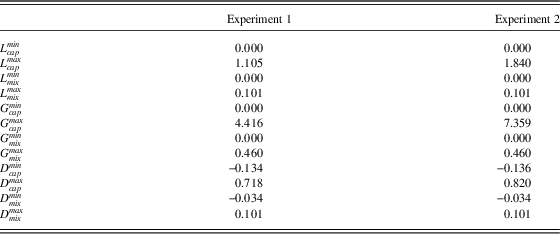
Agents using credit assignment structures L, G, G+PBRS and D were tested on this problem domain, as well as agents that randomly select actions from a uniform distribution as a baseline. In the case of L and G, the components of the reward vector are first normalized (Equation 10) using the utopia and nadir values given in Table 1, and then scalarized using a linear combination (Equation 9). The normalized and scalarized combinations are then used when updating an agents’ value function estimates (Equation 1).

Table 1

Normalization constants.

In the case of D, first each objective is shaped separately using its specific counterfactual value (Equations 19 and 20). The resultant shaped reward vector is then normalized (Equation 10) and scalarized (Equation 9) as above.

When applying PBRS, the global reward vector is first normalized (Equation 10) then scalarized (Equation 9), before adding the shaping reward F (Equation4) to the scalarized combination. Algorithm 4.1 shows the entire process that is followed when the agents in the MOBPD are rewarded with G+PBRS. The following two heuristics adapted from the work of Devlin et al. (Reference Devlin, Yliniemi, Kudenko and Tumer2014) were used to test the effect of PBRS:

• ∙ Middle: All agents are invited to a party at the middle beach section (b=2). This heuristic incorporates some basic knowledge about the optimal trade-off solutions, that is, the idea that one resource should be ‘sacrificed’ or congested by most of the agents for the greater good of the system. This shaping is expected to improve both the performance and learning speed of agents receiving PBRS, and will demonstrate the effect of PBRS when useful but incomplete domain knowledge is available.

  (21) $$\Phi (b){\equals}\left( {\matrix{ 1 &#x0026; {{\rm if}\; b{\equals}2} \cr 0 &#x0026; {{\rm otherwise}} \cr } } \right.$$

• ∙ Spread: The Spread heuristic encourages agents to distribute themselves evenly across the sections in the MOBPD. This is an example of a weak heuristic, and demonstrates the effect of PBRS in cases where very little useful domain knowledge is available. Therefore, agents receiving this shaping are expected to show modest if any improvements in learning speed and final performance.

(22) $$\eqaligno {\Phi (b){\equals}\left( {\matrix{ 1 &#x0026;\hskip-46pt {{\rm if}\;b{\equals}0{\rm ,}\;agent\_id\in[0,N/\mid B\mid\!{\minus}1]} \cr 1 &#x0026; \hskip-5pt {{\rm if}\;b{\equals}1{\rm ,}\;agent\_id\in[N/\mid B\mid\,,2N/\mid B\mid\!{\minus}1]} \cr 1 &#x0026; {{\rm if}\;b{\equals}2{\rm ,}\;agent\_id\in[2N / \mid B \mid \,,3N / \mid B \mid \!{\minus}1]} \cr 1 &#x0026; {{\rm if}\;b{\equals}3{\rm ,}\;agent\_id\in[3N / \mid B \mid\,,4N / \mid B \mid \!{\minus}1]} \cr 1 &#x0026; {{\rm if}\;b{\equals}4{\rm ,}\;agent\_id\in[4N / \mid B \mid \,, 5N / \mid B \mid \!{\minus}1]} \cr 0 &#x0026;\hskip-162pt {{\rm otherwise}} \cr } } \right.$$

where N is the total number of agents.

4.3 Experimental procedure

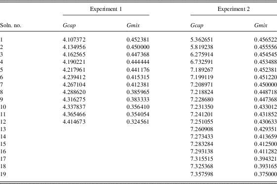
Two different empirical studies were conducted in the MOBPD. In the first experiment ψ=3, num_agents_M=35 and num_agents_F=15, while in the second experiment ψ=5, num_agents_M=70 and num_agents_F=30 in order to increase the complexity. Changing the parameters in this way produces separate, independent versions of the problem that each have a unique set of Pareto optimal system utilities. The sets of Pareto optimal utilities for both versions of the problem are listed in Table 2. These were determined by calculating G _cap and G _mix for each possible distribution of m and f agents among the beach sections, and then removing all dominated solutions. As the rewards for both objectives are normalized in the range [0, 1], an even weighting of [0.5, 0.5] was used when scalarizing objectives.

Table 2

Multi-objective beach problem domain (MOBPD) Pareto optimal system utilities

The number of sections is set to |B|=5, and the first num_agents_M/2 and num_agents_F/2 begin each episode at beach section 1, while the rest begin at beach section 3. The difficulty of this coordination problem could be increased further by assigning a random initial starting state to each agent at the beginning of each episode, rather than the fixed initial start states which are used in these experiments.

In all experiments, the number of episodes is set to num_episodes=10 000, the number of timesteps is set to num_timesteps=1, the learning rate is set to α=0.1, the exploration rate is set to ε=0.05 with epsilon_decay_rate=0.9999 and the discount factor is set to γ=0.9. These values were selected following parameter sweeps to determine the best performing values.

All plots include error bars representative of the standard error of the mean based on 50 statistical runs. Specifically, the error is calculated as $$\sigma \,/\,\sqrt n $$ where σ is the standard deviation and n is the number of statistical runs. Error bars are included on all plots at 1000 episode intervals. The plots show the average performance across the 50 statistical runs that were conducted at 10 episode intervals. All claims of statistical significance are supported by two-tailed t-tests assuming unequal variances, with p=0.05 selected as the threshold for significance.

4.4 Experimental results

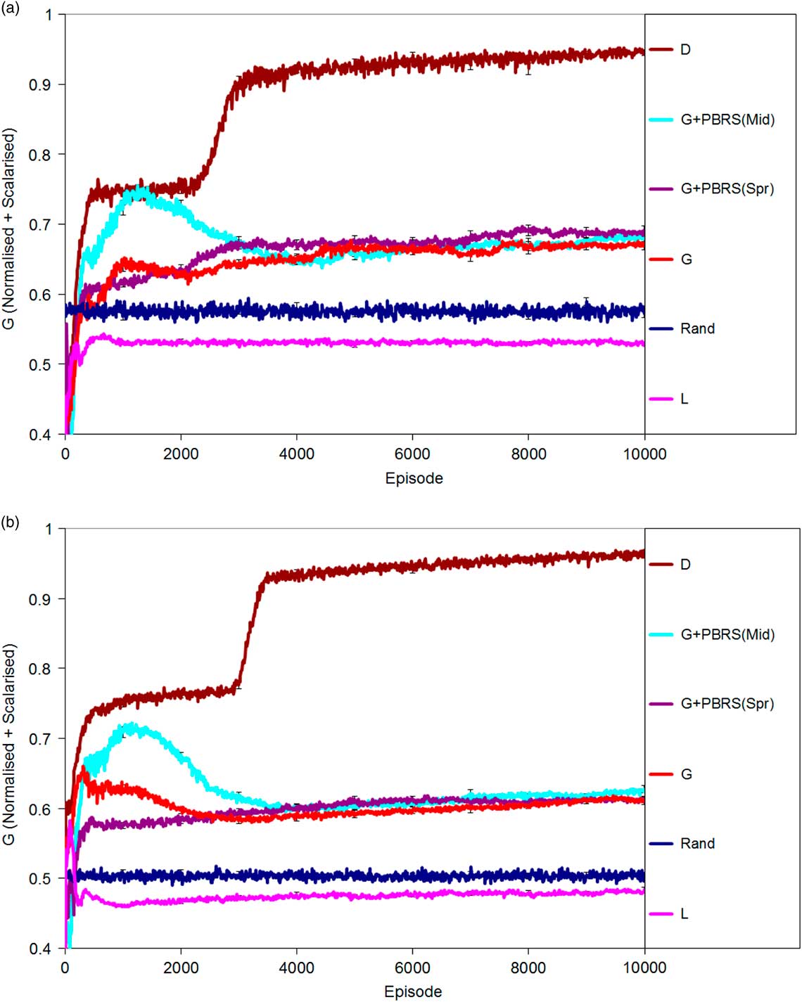
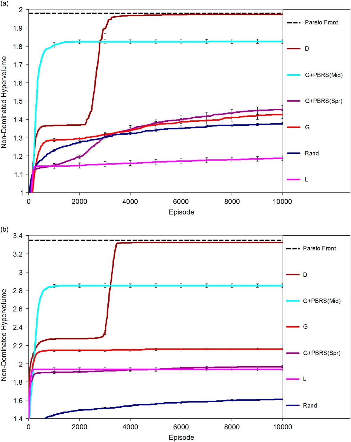
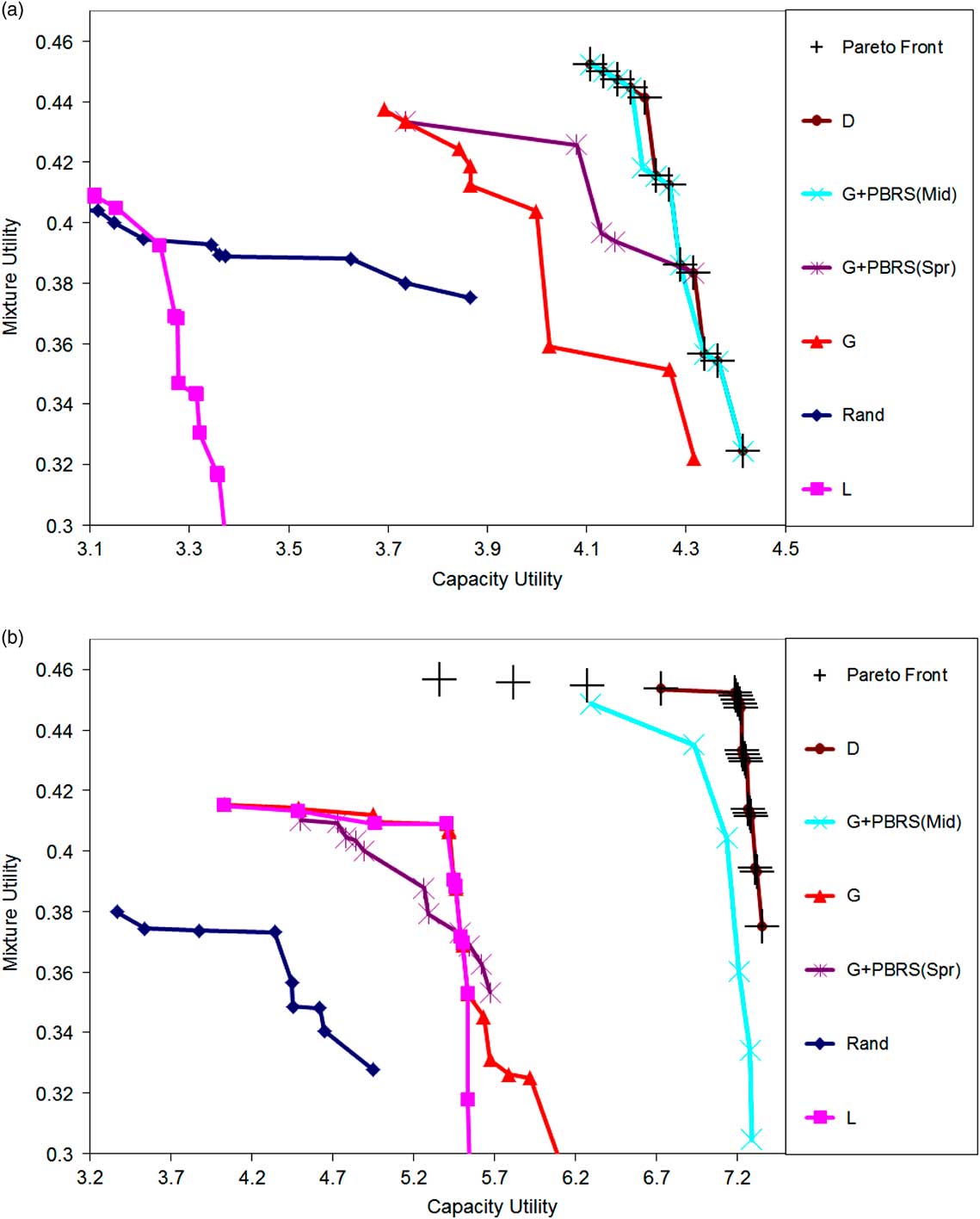
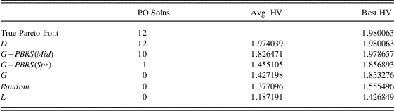
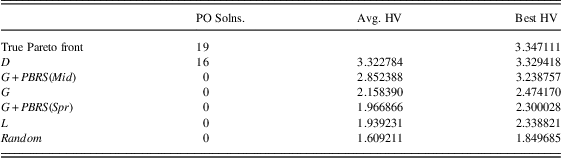
The results for both experiments are summarized in Tables 3 and 4. These tables list the number of true Pareto optimal solutions found across all runs (PO Solns.), the average hypervolume of the non-dominated solutions found on each statistical run (Avg. HV), and the hypervolume of the best non-dominated solutions found across all runs (Best HV). Best HV gives an indication of how close an approach can get to finding the true Pareto front of the problem, while Avg. HV shows how consistent the performance of an approach is. Figure 2a and 2b show the average performance on the normalized scalarized global reward, while Figure 3a and 3b show the average hypervolume of the non-dominated solutions found on each run. The best non-dominated solutions found by each approach over all runs, as well as the true Pareto fronts are shown in Figure 4a and 4b.

Figure 2

Average performance on normalized scalarized global reward

Figure 3

Average hypervolume of non-dominated solutions found

Figure 4

Best non-dominated episodes over all runs

Table 3

Experiment 1 results.

PBRS=potential-based reward shaping; PO=Pareto optimal solutions; HV=hypervolume.

Table 4

Experiment 2 results.

PBRS=potential-based reward shaping; PO=Pareto optimal solutions; HV=hypervolume.

D offered the best overall performance in both experiments, sampling all 12 Pareto optimal solutions in the first experiment, and 16 of 19 in the second experiment. G+PBRS(Middle) sampled 10 Pareto optimal solutions in the first experiment, and none in the second. G+PBRS(Spread) sampled a single Pareto optimal solution in the first experiment, and none in the second. Both of the typical MARL credit assignment structures L and G, as well as the random baseline failed to find any true Pareto optimal solutions. This highlights the fact that in even the simplest of multi-objective multi-agent problems, G alone may not be sufficiently informative to allow agents to find solutions that form part of the true Pareto optimal set, therefore justifying the need for more sophisticated credit assignment techniques.

Figure 2a and 2b give an indication of the relative learning speed of the different approaches, measured using the return from the normalized scalarized system evaluation function. This metric measures the learning performance in terms of the unshaped system evaluation functions. A score of 1.0 represents the theoretical maximum upper bound on performance in the domain being achieved on both objectives simultaneously. The value 1.0 is never reachable however, as the two objectives are in conflict (it is not possible to score the maximum on each objective simultaneously).

It is important to note that in this domain, relatively few agents selecting actions which are not Pareto optimal could have a large effect on the G(normalized+scalarized) metric; this contributes to the difficulty of the coordination problem. D again offers the best performance on the G(normalized+scalarized) metric, although G+PBRS(Middle) almost matches it in the early episodes. As expected, L performs poorly here, as it does not encourage all agents to act in the system’s best interest. G+PBRS(Spread) performs poorly compared to G+PBRS(Middle); as is the case in single-objective SGs, poorly designed potential functions with misleading information can damage system performance.

The effect of using a decreasing exploration rate is also evident in Figure 2a and 2b. In the early episodes, D has already learned useful information about the how Pareto optimal solutions may be reached (having lots of agents in the middle, and relatively few agents of both types in the remaining sections). As the exploration rate is reduced, the performance of D increases as close to all agents will now be able to select the optimal action, whereas in earlier episodes more agents were forced to select sub-optimal actions due to the higher exploration probability. With G+PBRS(Middle) most of the agents initially learn to go to the middle state; here a high exploration rate is beneficial while it encourages enough agents to select actions which take them away from this state. However, the proportion of agents which select these random actions decreases as time goes on. In the case of L and G, miscoordination and credit assignment deficiencies again become problematic. Even if an agent explores and selects a new action which benefits performance, another agent could select an action which damages performance at the same time; however, both agents get the same reward, regardless of whether they improved system performance. So, we should expect L and G to converge to suboptimal points of equilibrium eventually, even if they begin with higher performance initially. The effect of inadequate credit assignment becomes more serious in larger MAS, which is why it is more evident in the 100 agent test domain than in the 50 agent test domain.

In Figure 3a and 3b it is clear that G+PBRS(Middle) samples a lot of solutions that are close to the Pareto front in the early stages of both experiments, resulting in a high hypervolume calculation, and initially beating the performance of D. This demonstrates the beneficial effect that PBRS with a suitable heuristic can have on the agents’ exploration. D initially samples promising solutions more slowly, but by the end of each experiment it has reached an average hypervolume very close to that of the true Pareto front (shown with a black dashed line in both plots). In terms of average hypervolume reached, D offers statistically better performance than G+PBRS(Middle) in both experiment 1 (p=1.11×10⁻¹⁷) and experiment 2 (p=2.67×10⁻²⁹). G+PBRS(Middle) does however offer a statistically significant increase in performance over unshaped G on this metric in the first experiment (p=1.61×10⁻²⁶) and the second experiment (p=6.79×10⁻⁴⁷).

Figure 4a and 4b show that the best non-dominated solutions found by D and G+PBRS(Middle) match very closely with those of the true Pareto front in both experiments. The solutions found by L and G are dominated by those found by D and G+PBRS(Middle); these typical MARL credit assignment structures are not informative enough to guide agents towards good solutions in the MOBPD.

The performances of D and G+PBRS(Middle) demonstrate that well designed reward shaping techniques can guide agents towards the true Pareto optimal solutions in MOSGs by making G more informative. Thus the issue of appropriate credit assignment is just as important in MOSGs as it is in traditional single-objective SGs. Furthermore, the results for D and G+PBRS(Middle) offer the first supporting empirical evidence that both D and PBRS preserve the true Pareto optimal sets of solutions in MOSGs. In the second experiment, both approaches do not perform as well due to the increased complexity of the problem. In the case of PBRS, more suitable heuristics could be designed to improve performance, although G+PBRS(Middle) performs extremely well considering the simple nature of the information that is provided.

5.1 Dynamic Economic Emissions Dispatch

The version of the DEED problem which will be used for this study was originally proposed by (Basu, Reference Basu2008). Basu’s version is presented as a multi-dimensional optimization problem, with each dimension in the problem space representing the power output of a generator at a given time. The cost function f ₁ which computes the total fuel cost for the generators, including the effect of valve point loading (Walters & Sheble, Reference Walters and Sheble1993), is defined as:

(23) $$f_{1} {\equals}\mathop{\sum}\limits_{m{\equals}1}^M \mathop{\sum}\limits_{n{\equals}1}^N [a_{n} {\plus}b_{n} P_{{nm}} {\plus}c_{n} (P_{{nm}} )^{2} {\plus}\,\mid\,d_{n} sin\{ e_{n} (P_{n}^{{min}} {\minus}P_{{nm}} )\} \,\mid\,]$$

where M=24 is the number of hours, N=10 is the number of power generators, a _n , b _n , c _n , d _n and e _n are the cost coefficients associated with each generator n, P _nm is the power output from generator n at time m, and $$P_{n}^{{min}} $$ is the minimum permissible power output of generator n.

The total combined emissions of SO ₂ and NO from the group of generators is calculated using function f ₂ (Basu, Reference Basu2008):

(24) $$f_{2} {\equals}\mathop{\sum}\limits_{m{\equals}1}^M \mathop{\sum}\limits_{n{\equals}1}^N [\alpha _{n} {\plus}\beta _{n} P_{{nm}} {\plus}\gamma _{n} (P_{{nm}} )^{2} {\plus}\eta \exp \delta P_{{nm}} ]$$

where α _n , β _n , γ _n , η _n and δ _n are the emission coefficients associated with each generator n.

The total power output in a given hour must be equal to the sum of the power demand and transmission losses:

(25) $$\mathop{\sum}\limits_{n{\equals}1}^N P_{{nm}} {\equals}P_{{Dm}} {\plus}P_{{Lm}} \quad \quad \forall m\in M$$

where P _Dm is the power demand over hour m and P _Lm is the transmission loss over hour m.

There are two inequality constraints which any potential solutions are subject to: the operating limits and the ramp limits for each power generator in the station. The operating limits specify the minimum and maximum possible power output of a generator, while the ramp limits determine the maximum allowed increase or decrease in the power output of a generator from one hour to the next.

(26) $$P_{n}^{{min}} \leq P_{{nm}} \leq P_{n}^{{max}} $$

(27a) $$P_{{nm}} {\minus}P_{{n(m{\minus}1)}} \leq UR_{n} $$

(27b) $$P_{{n(m{\minus}1)}} {\minus}P_{{nm}} \leq DR_{n} $$

where $$P_{n}^{{min}} $$ and $$P_{n}^{{max}} $$ refer to the minimum and maximum power output of each generator, P _nm is the power output for n∈N and m∈M, and UR _n and DR _n are the ramp up and ramp down limits for generator n.

In order to satisfy the equality constraint described by Equation (25), the first generator n=1 is a slack generator. The power outputs of the other 9 generators are set directly, and the slack generator makes up any shortfall in the combined power output. The settings for the slack generator are therefore dependant variables during the optimization process, while the outputs of the other N−1 generators are independent variables. The power output of the slack generator for a single hour, P _1m , may be calculated by rearranging Equation (25):

(28) $$P_{{1m}} {\equals}P_{{Dm}} {\plus}P_{{Lm}} {\minus}\mathop{\sum}\limits_{n{\equals}2}^N P_{{nm}} $$

The loss in the transmission lines between generators, P _Lm , over hour m is calculated as follows:

(29) $$P_{{Lm}} {\equals}\mathop{\sum}\limits_{n{\equals}2}^N \mathop{\sum}\limits_{j{\equals}2}^N P_{{nm}} B_{{nj}} P_{{jm}} {\plus}2P_{{1m}} (\mathop{\sum}\limits_{n{\equals}2}^N B_{{1n}} P_{{nm}} ){\plus}B_{{11}} (P_{{1m}} )^{2} $$

where B is the matrix of transmission line loss coefficients (Basu, Reference Basu2008).

Combining Equation (29) with Equation (30) produces the following quadratic equation:

(30) $$\matrix{ 0 \hfill &#x0026; {{\equals}B_{{11}} (P_{{1m}} )^{2} {\plus}(2\mathop{\sum}\limits_{n{\equals}2}^N B_{{1n}} P_{{nm}} {\minus}1)P_{{1m}} {\plus}} \hfill \cr {} \hfill &#x0026; {(P_{{Dm}} {\plus}\mathop{\sum}\limits_{n{\equals}2}^N \mathop{\sum}\limits_{j{\equals}2}^N P_{{nm}} B_{{nj}} P_{{nm}} {\minus}\mathop{\sum}\limits_{n{\equals}2}^N P_{{nm}} )} \hfill \cr } $$

Solving this quadratic equation using basic algebra will give the reactive power of the slack generator, P _1m , at each hour. All required values for the cost coefficients, emission coefficients, ramp limits, generator capacity limits, power demands and transmission line loss coefficients can be found in the work of (Basu, Reference Basu2008).

5.2 DEED as a MOSG

In order to create a version of the DEED problem suitable for the application of MARL, it can be reformulated as a MOSG. The problem is divided into one of sequential decision making, where each hour m∈M is a separate timestep in the SG. Each of the nine directly controlled generators n={2,...,10} are assigned to an agent i={2,...,10}, where agent i sets the power output P _nm of its generator n=i at every timestep m.

It is now necessary to derive new cost and emissions functions, which will measure the system utility at each timestep. From Equation (23), a function $$f_{c}^{L} $$ may be derived which computes the local cost for generator n over hour m:

(31) $$f_{c}^{L} (n,m){\equals}a_{n} {\plus}b_{n} P_{{nm}} {\plus}c_{n} (P_{{nm}} )^{2} {\plus}\,\mid\,d_{n} sin\{ e_{n} (P_{n}^{{min}} {\minus}P_{{nm}} )\} \,\mid\,$$

Thus the global cost function $$f_{c}^{G} $$ for all generators over hour m is:

(32) $$f_{c}^{G} (m){\equals}\mathop{\sum}\limits_{n{\equals}1}^N f_{c}^{L} (n,m)$$

Similarly, from Equation (24) an emissions function $$f_{e}^{L} $$ may be developed for generator n over hour m:

(33) $$f_{e}^{L} (n,m){\equals}E(\alpha _{n} {\plus}\beta _{n} P_{{nm}} {\plus}\gamma _{n} (P_{{nm}} )^{2} {\plus}\eta \exp \delta P_{{nm}} )$$

where E=10 is the emissions scaling factor, chosen so that the magnitude of the local emissions function $$f_{e}^{L} $$ matches that of the local cost function $$f_{c}^{L} $$ . It follows that the global emissions function $$f_{e}^{G} $$ for all generators over hour m is:

(34) $$f_{e}^{G} (m){\equals}\mathop{\sum}\limits_{n{\equals}1}^N f_{e}^{L} (n,m)$$

The next environmental state for each agent i is defined as a vector containing the change in power demand ΔP _D since the previous timestep, and the previous power output of the generator n, P _nm . The change in power demand at time m is calculated as:

(35) $$\Delta P_{{Dm}} {\equals}P_{{Dm}} {\minus}P_{{D(m{\minus}1)}} $$

Therefore the state vector for agent i (controlling generator n) at time m is:

(36) $$s_{{i,m}} {\equals}[\Delta P_{{Dm}} ,P_{{n(m{\minus}1)}} ]$$

The action chosen by agent i at each timestep determines the power output of the generator n under its control. However, the power output constraints in Equation (26) must be satisfied for each generator. Therefore the possible action set for agent i consists of:

(37) $$A_{i} {\equals}\{ P_{n}^{{min}} ,...,P_{n}^{{max}} \} $$

At any hour m, when the ramp limits in Equations (27) and (28) are imposed, an agent’s action set is constrained to:

(38) $$A_{{im}} {\equals}\{ P_{{n(m{\minus}1)}} {\minus}UR_{n} \geq P_{n}^{{min}} ,...,P_{{n(m{\minus}1)}} {\minus}UR_{n} \leq P_{n}^{{max}} \} $$

It is also necessary to consider the power limits and ramp limits of the slack generator, n=1. A global penalty function $$f_{p}^{G} $$ based on the static penalty method (Smith et al., Reference Smith, Coit, Baeck, Fogel and Michalewicz2000) is used to capture violations of these constraints:

(39) $$f_{p}^{G} (m){\equals}\mathop{\sum}\limits_{v{\equals}1}^V C(\,\mid\,h_{v} {\plus}1\,\mid\,\delta _{v} )$$

(40) $$h_{1} {\equals}\left( {\matrix{ {P_{{1m}} {\minus}P_{1}^{{max}} } &#x0026; {{\rm if}\;P_{{1m}} \,\gt\,P_{1}^{{max}} } \cr {P_{1}^{{min}} {\minus}P_{{1m}} } &#x0026; {{\rm if}\;P_{{1m}} \,\lt\,P_{1}^{{min}} } \cr 0 &#x0026; {{\rm otherwise}} \cr } } \right.$$

(41) $$h_{2} {\equals}\left( {\matrix{ {(P_{{1m}} {\minus}P_{{1(m{\minus}1)}} ){\minus}UR_{1} } &#x0026; {{\rm if}\;(P_{{1m}} {\minus}P_{{1(m{\minus}1)}} )\,\gt\,UR_{1} } \cr {(P_{{1m}} {\minus}P_{{1(m{\minus}1)}} ){\plus}DR_{1} } &#x0026; {{\rm if}\;(P_{{1m}} {\minus}P_{{1(m{\minus}1)}} )\,\lt\,{\minus}DR_{1} } \cr 0 &#x0026; {{\rm otherwise}} \cr } } \right.$$

where |V|=2 is the number of constraints handled using this method (one possible violation each for slack generator power and ramp limits over hour m), C=10E6 is the violation constant, h _v is the violation of each constraint, and δ _v =0 if there is no violation in a given constraint and δ _v =1 if the constraint is violated. The violation constant C=10E6 was selected so that the output of the penalty function will have a similar magnitude to that of the cost function $$f_{c}^{G} $$ . The penalty function is an additional objective that must be optimized, in addition to cost and emissions.

The counterfactual cost, emissions and violations terms for an agent i are calculated by assuming that the agent did not choose a new power output value in the timestep m (i.e. the power output of generator n=i did not change). This assumed action of holding the same power output is chosen based on the intuition that the counterfactual for a timestep m should represent the system’s performance without the effect of agent i's action selection.

(42) $$f_{c}^{{G({\minus}i)}} (m){\equals}\mathop{\sum}\limits_{{\scriptstyle n{\equals}1 \atop \scriptstyle n\,\ne\,i} }^N f_{c}^{L} (n,m){\plus}f_{c}^{L} (i,m{\minus}1)$$

(43) $$f_{e}^{{G({\minus}i)}} (m){\equals}\mathop{\sum}\limits_{{\scriptstyle n{\equals}1 \atop \scriptstyle n\,\ne\,i} }^N f_{e}^{L} (n,m){\plus}f_{e}^{L} (i,m{\minus}1)$$

where $$f_{c}^{{G({\minus}i)}} (m)$$ is the counterfactual cost term and $$f_{e}^{{G({\minus}i)}} (m)$$ is the counterfactual emissions term. The output of the counterfactual version $$f_{p}^{{G({\minus}i)}} $$ of the penalty function $$f_{p}^{G} $$ is calculated as per Equation (40), with the term $$P_{{1m}}^{{({\minus}i)}} $$ substituted for P _1m in Equations (41) and (42). $$P_{{1m}}^{{({\minus}i)}} $$ is calculated as:

(44) $$P_{{1m}}^{{({\minus}i)}} {\equals}P_{{Dm}} {\plus}P_{{Lm}} {\minus}\mathop{\sum}\limits_{{\scriptstyle n{\equals}2 \atop \scriptstyle n\,\ne\,i} }^N P_{{nm}} {\minus}P_{{i(m{\minus}1)}} $$

5.3 Action selection

In initial experimental work on the DEED MOSG using the full action definitions in Equations (38) and (39), the quality of the policies learned was highly variable, often resulting in poor performance. This may be attributed to the fact that the action space A _i for each agent is of a different size. For example, using a discretization level of 1MW, the smallest action space has 46 actions, and the largest has 321 actions when using the generator operating limits specified by (Basu, Reference Basu2008). These discrepancies meant the time required for each agent to sample the full state-action space varied widely. To overcome this difficulty, an abstraction A ^* of the action space will be used, where each agent has a set of 101 possible actions A ^*={0, 1, ..., 99, 100}. Each action represents a different percentage value of the operating range of the generator, so generators with wider operating ranges have larger increments. The power output from generator n for action $$a_{i}^{{\asterisk}} $$ is calculated as:

(45) $$P_{n} {\equals}P_{n}^{{min}} {\plus}a_{i}^{{\asterisk}} \left( {{{P_{n}^{{max}} {\minus}P_{n}^{{min}} } \over {100}}} \right)\quad \quad i{\equals}n$$

The power output selected by an agent is still subject to the ramp limits, as per Equations (27), (28) and (39), so a ^* selections that would violate these limits are not allowed. This action space abstraction is used in all experimental work presented in this study. Agents select actions from A ^* using the ε-greedy strategy.

5.4 Applying MARL

Multiple individual Q-learning agents were tested in the DEED MOSG defined above, learning with credit assignment structures L, G, G+PBRS, and D. All reward vectors are scalarized using either a linear scalarization (Equation 9) with the following objective weights: w _c =0.225, w _e =0.275, and w _p =0.5. These objective weights were chosen following parameter sweeps, so as to maintain a good balance between the objectives. The agents receive one of these scalarized reward signals while learning: L, G, G+PBRS, or D.

Note that in the case of a local reward L, the number of objectives |C|=2 as there is no local penalty function. |C|=3 for all other credit assignment schemes, as they all make use of the global versions of the objective functions. Note also that the rewards assigned are negative, as all objectives must be minimized.

In the case of D, each objective is first shaped separately using its specific counterfactual value (Equations 43, 44 and 45) before being scalarized. When applying G+PBRS, the global reward vector is first scalarized, before adding the shaping reward F (Equation 4) to the scalarized combination. Three different heuristics adapted from (Mannion et al., Reference Mannion, Devlin, Mason, Duggan and Howley2017b) were used to test the effectiveness of PBRS in this problem domain:

• ∙ High: All agents are encouraged to select high power values. This heuristic is expected to quickly reduce the cost and emissions values during learning, and lead to good solutions.

  (46) $$\Phi _{{High}} (i,m){\equals}{\minus}(100{\plus}({{P_{{n,m{\minus}1}} {\minus}P_{n}^{{min}} } \over {P_{n}^{{max}} {\minus}P_{n}^{{min}} }}{\times}100)){\times}10^{6} \quad \quad i{\equals}n$$

• ∙ Low: All agents are encouraged to select low power values. This heuristic is also expected to increase learning speed, although encouraging agents to select low power values will increase loading on the slack generator, which may negatively affect the running costs and emissions produced.

  (47) $$\Phi _{{Low}} (i,m){\equals}{\minus}(100{\minus}({{P_{{n,m{\minus}1}} {\minus}P_{n}^{{min}} } \over {P_{n}^{{max}} {\minus}P_{n}^{{min}} }}{\times}100)){\times}10^{6} \quad \quad i{\equals}n$$

• ∙ Mixed: This heuristic encourages a mixture of the two different behaviours above. The agents i=2 to i=5 are encouraged to select low power values using the low heuristic, whereas the agents from i=6 to i=10 are encouraged to select high power values using the high heuristic. The design of this mixed heuristic is based on the intuition that it may be beneficial to keep some generators in a group working at close to full power continuously to satisfy the baseline power demand, while the rest of the generators will only increase their power output during peaks of high demand.

(48) $$\Phi _{{Mixed}} (i,m){\equals}\left( {\matrix{ {\Phi _{{Low}} (i,m)} &#x0026; {{\rm if}\;i\leq 5} \cr {\Phi _{{High}} (i,m)} &#x0026; {{\rm otherwise}} \cr } } \right.$$

5.5 Experimental procedure

Experiments were conducted on two different variations of the DEED MOSG. In the normal version of the problem, the agents learn for 20 000 episodes, each of which comprises 24 hours. The second version also lasts for 20 000 episodes; after 10 000 episodes a random generator n∈{2,...,10} fails, and the agents must learn to compensate for the loss of this generator, while still meeting the same electricity demand. The aim of this second experiment is to test the robustness to disturbances and adaptability of agents learning using each MARL credit assignment structure.

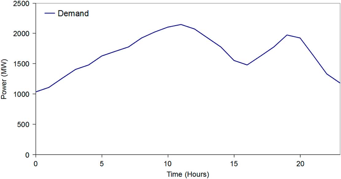
The demand profile used in both experiments is shown in Figure 5. This is the same demand profile that was used in used in work by Basu (Reference Basu2008) and Mason (Reference Mason2015), so the DEED MOSG results will be directly comparable to results reported by these authors. The learning parameters for all agents are set as follows: α=0.10, γ=0.75, ε=0.05. These values were selected following parameter sweeps to determine the best performing settings.

Figure 5

Twenty-four-hour power demand

5.6 Experimental results

We will first discuss the results of the standard version of the problem. All plots include error bars at 1000 episode intervals representative of the standard error of the mean based on 50 statistical runs. Specifically, the error is calculated as $$\sigma \,/\,\sqrt n $$ where σ is the standard deviation and n is the number of statistical runs. The plots show a 200 episode moving average across the 50 statistical runs that were conducted. All claims of statistical significance are supported by two-tailed t-tests assuming unequal variances, with P=0.05 selected as the threshold for significance.

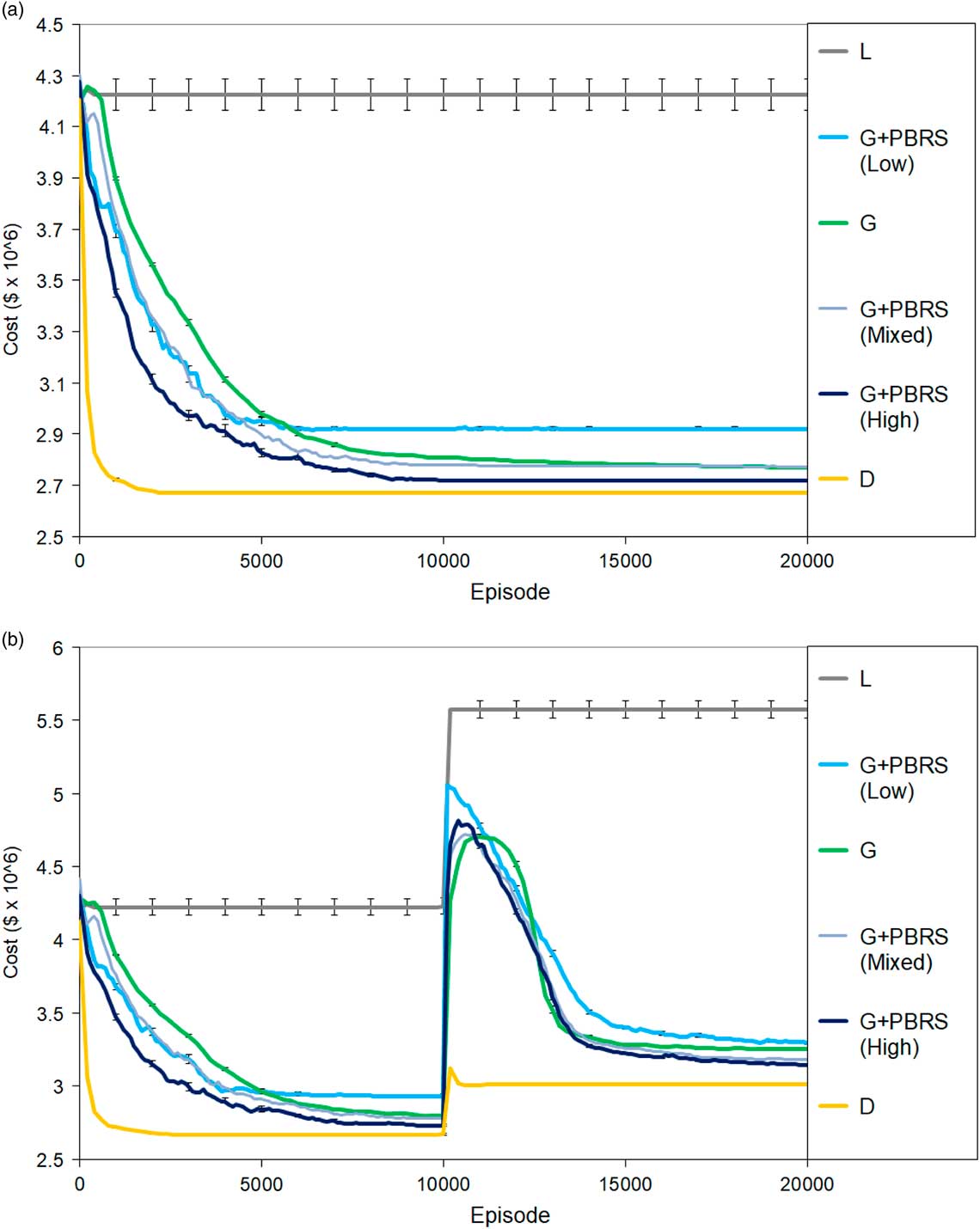
The plots of learning curves for the cost objective in the first experiment (Figure 6) give an indication of the relative learning speeds and stability of performance for each of the approaches tested. As expected, L performs poorly here, as the local reward encourages agents to greedily minimize their own fuel cost, without considering the utility of the system as a whole. D converges to a stable policy most quickly, while G also learns good policies, but at a slower rate than D.

Figure 6

Learning curves for the cost objective

G+PBRS(High) and G+PBRS(Mixed) both learn more quickly than G. G+PBRS(Low) also initially learns more quickly than G; however, it does so at the expense of damaging final performance when compared to unshaped G. Here it can be seen again that the characteristic effects of PBRS in SGs are preserved in MOSGs; well designed heuristics can improve learning speed and final performance in MOSGs, while poorly designed heuristics may damage learning speed and final performance.

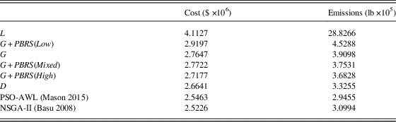
Table 5 displays the average cost and emissions for the MARL approaches tested, along with NSGA-II results reported by Basu (Reference Basu2008) and PSO-AWL (avoidance of worst locations) results reported by Mason (Reference Mason2015) for comparison purposes. In this table, the cost is presented in $ ×10⁶ and the emissions are presented in lb ×10⁵. All values in the table are rounded to 4 decimal places.

Table 5

DEED average final performance.

AWL=avoidance of worst locations; DEED=dynamic economic emissions dispatch; PBRS=potential-based reward shaping; PSO=particle swarm optimization.

The differences in the mean final performance of D and G were found to be significant for both the cost objective (p=5.01×10⁻²²), and the emissions objective (p=3.20×10⁻¹⁰). D also performed statistically better than G+PBRS(High) on both the cost objective (p=1.06×10⁻⁸) and the emissions objective (p=7.01×10⁻¹⁶). G+PBRS(High) performed statistically better than G in terms of cost (p=2.99×10⁻¹⁰) and emissions (p=2.63×10⁻⁴), while G+PBRS(Mixed) was statistically the same as G in terms of cost (p=0.398), and statistically better in terms of emissions (p=2.61×10⁻³). The misleading shaping G+PBRS(Low) caused a significant drop in average performance when compared with G in terms of both cost (p=1.13×10⁻³³) and emissions (p=1.7×10⁻⁶).

Analysing the average results presented in Table 5, the best MARL approach produces results that are comparable to those of GA and PSO based approaches, although not quite as good. For example, Basu’s NSGA-II has 4.2% lower costs, and 6.8% lower emissions than D on average in this problem. However, MAS is arguably a more interesting paradigm to use when studying these types of optimization problems, due to the ability to modify simulation parameters while learning online, and the possibility of modelling system disturbances (e.g. generator failure). MAS are inherently suited to distributed control and optimization problems like DEED, and the information learned by the agents can be used to compute new policies online if the parameters of the problem change, unlike the GA and PSO based approaches.

Figure 6b shows the learning curves for the cost objective in the second experiment, where a random generator fails. L again performs poorly in this experiment. D is again the best performing reward structure here, converging to a stable joint policy after generator failure much more quickly than any other reward structure tested. The agents learning using D are exceptionally robust to disturbances in this problem domain when compared to agents learning using the other credit assignment structures. Agents learning using G+PBRS(High) and G+PBRS(Mixed) again outperform agents using unshaped G in this experiment, learning to adapt to generator failure more quickly, and converging to better joint policies on average.

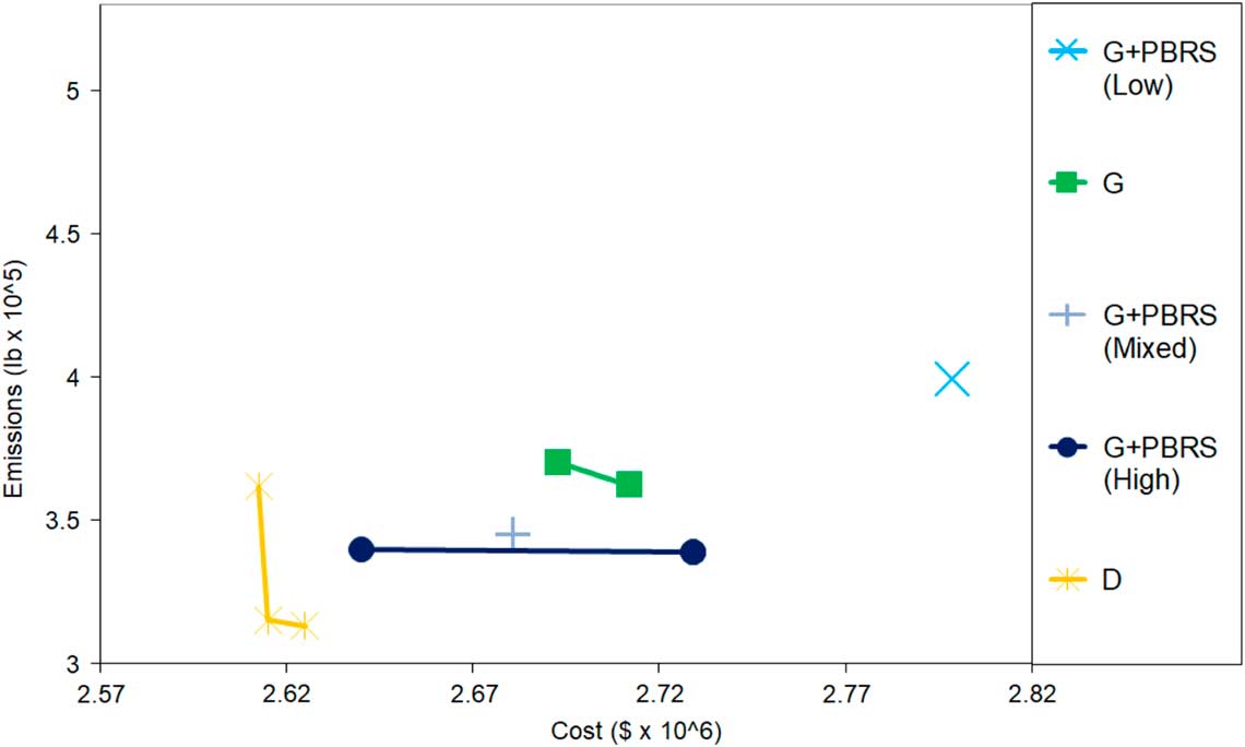
Figure 7 plots the Pareto fronts for the best performing credit assignment structures tested. These fronts are comprised of the best non-dominated episodes produced by each approach over 50 runs conducted in the first experiment. D again offers the best performance here, sampling solutions that Pareto dominate those found by all other approaches. G+PBRS(High) is the next best performer, with one of its episodes Pareto dominating those of all other approaches except those of D. G+PBRS(Mixed) also produced a solution that Pareto dominated all episodes produced by unshaped G; these results again confirm that as well as learning more quickly, agents receiving PBRS with a well designed heuristic can also significantly outperform agents learning using unshaped G in MOSGs. Finally, the misleading information encoded in G+PBRS(Low) damaged the performance of agents receiving it, evidenced by the fact that all of its episodes are Pareto dominated by unshaped G.

Figure 7

Best non-dominated episodes over all runs

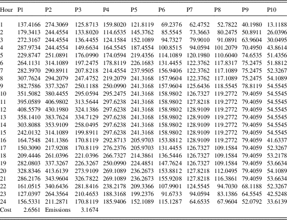
A sample 24 hour generator schedule produced by D is presented in Table 6, showing the outputs in MW of the 9 controlled generators (P2 to P10), and the slack generator (P1). Sample generator schedules for GA and PSO approaches are available in the work of Basu (Reference Basu2008) and Mason (Reference Mason2015).

Table 6

Sample solution produced by D.