1 Introduction
In critical systems, software is often considered as the weakest link of the chain and there are many stories of software bugs that yield catastrophic consequences. For instance, on September 14, 2004, L. Geppert reportsFootnote 1 that the contact voice lost of Los Angeles air traffic controllers was due to a software bug that resulted to an unexpected shutdown of the Voice Switching and Control System. It turned out that shutdown was due to a 32-bit integer value running out of digits. Hopefully, in a situation that could have proved deadly, tragedy was avoided not only by both pilots and controllers professionalism, but also by another software-based critical system: the Traffic Alert and Collision Avoidance System (TCAS), which is embedded on aircraft to prevent from mid-air collisions. Thus, small software bugs can result to catastrophic situations and therefore, they must be tracked and eliminated from critical systems.
In the Avionics domain, software verification currently includes manual code review and analysis, unit testing, software and hardware integration testing and validation testing. These various tasks address distinct non-redundant verification levels and offer reasonable confidence in terms of correction, reliability and performance. Code reviews consist in reading and discussing code written by other developers and help checking assertions derived from safety-critical properties. Unit testing consists in executing pieces of code (units) in isolation of the rest of the system with the intent of finding bugs. Test cases are selected from the input domain and used to exercise the software unit; then, a test verdict (either pass or fail) is produced by an oracle procedure to check the computed results. For testing software units in isolation, stubs have to be created to replace actual function calls. Software integration testing aims at testing the interaction between units and it is performed just by removing the stubs. Hardware integration testing consists in executing the code in its operational and physical environment. For avionics software, it means executing cross-compiled code on hardware emulators or embedded targets. Finally, validation testing aims at verifying high-level requirements through simulations and operational scenarios. As a consequence of the increasing complexity of avionics software, it is usually acknowledged that these techniques can hardly scale-up (Randimbivololona, Reference Randimbivololona2001). Code reviews are human-based approaches that highly depend on the confidence of reviewers. Testing is faced with combinatorial explosion and manual test data generation rapidly becomes too hard. In addition, test data selection and oracle production are error-prone processes that require competent and experienced engineers.
In our work, we explore the capabilities of Constraint Programming (CP) for automating parts of the software verification process. For several years, we have concentrated our efforts on automating the test case generation process by using dedicated constraint solving procedures. Initially, we proposed using classical constraint propagation with bound-consistency filtering and labeling for handling integer computations (Gotlieb et al., Reference Gotlieb, Botella and Rueher2000) and floating-point computations (Botella et al., Reference Botella, Gotlieb and Michel2006). Then, we refined the solving procedure with linear relaxations (Denmat et al., Reference Denmat, Gotlieb and Ducasse2007b) and dedicated global constraint approaches (Denmat et al., Reference Denmat, Gotlieb and Ducasse2007a). We also addressed the extension of our approach to pointer variables (Gotlieb et al., Reference Gotlieb, Denmat and Botella2007) and dynamic allocated structures. Recently, we have started to explore software verification with this approach and this paper mainly reports on our first experience in this matter.
In this paper, we present a general constraint solving procedure that combines bound-consistency filtering with Linear Programming (LP) over the rationals for solving disjunctive constraint systems over bounded integers. These constraint systems are extracted from imperative programs and correspond to various test data generation and verification tasks. The procedure dynamically combines constraint propagation and simplex solver calls in an iterating process that is coordinated by synchronization conditions. These conditions are based on simple integer cutting planes and domain pruning. The originality of this procedure over existing approaches comes from its ability to deal with nonlinear constructs such as disjunctions (including conditional constraints and reification), variables multiplication, Euclidian division and modulo. This paper also presents the results of an experiment on the application of this procedure to the verification of a software component of the TCAS. For this experiment, we used a publicly available implementation of the main component of TCAS that is responsible for alerts and Resolution Advisories (RAs) issuance. Our results show that using CP for automated verification of software units is viable and efficient.
The rest of the paper is organized as follows. The following section presents the TCAS. Section 3 describes the constraint solving procedure based on linear relaxation and cooperation between a finite domain (FD) solver and a LP solver. Section 4 presents our implementation while Section 5 discusses of experimental results and related works. Finally, Section 6 concludes the paper and draws some perspectives.
2 Traffic alert and collision avoidance system software verification
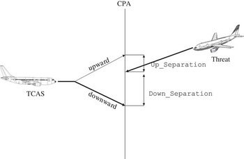
The TCAS is an on-board aircraft conflict detection and resolution embedded system. The system is intended to alert the pilot to the presence of nearby aircraft that pose a mid-air collision threat and to propose maneuvers so as to resolve these potential conflicts. In cases of collision threats, TCAS estimates the time remaining until the two aircrafts reach the closest point of approach (CPA) and presents two main levels of alert. As shown on Figure 1, when an intruder aircraft enters a protected zone, the TCAS issues a Traffic Advisory (TA) to inform the pilot of potential threat. If the danger of collision increases then a RA is issued, providing the pilot with a proposed maneuver that is likely to solve the conflict. The RAs issued by TCAS are currently restricted to the vertical plane only (either climb or descend) and their computation depends on time-to-go to CPA, range and altitude tracks of the intruderFootnote 2. Any TCAS implementation must be certified under level B of the DO-178B standardFootnote 3 (DO-178B, 1992). According to the standard, certifying TCAS requires to show that all the executable statements and decisions of the source code has been executed at least once during the testing phase. In addition, any non-executable statement must be removed from the source code because these statements do not trace back to any software requirements and do not perform any required functionality.
TCAS (Traffic Alert and Collision Avoidance System) alarms

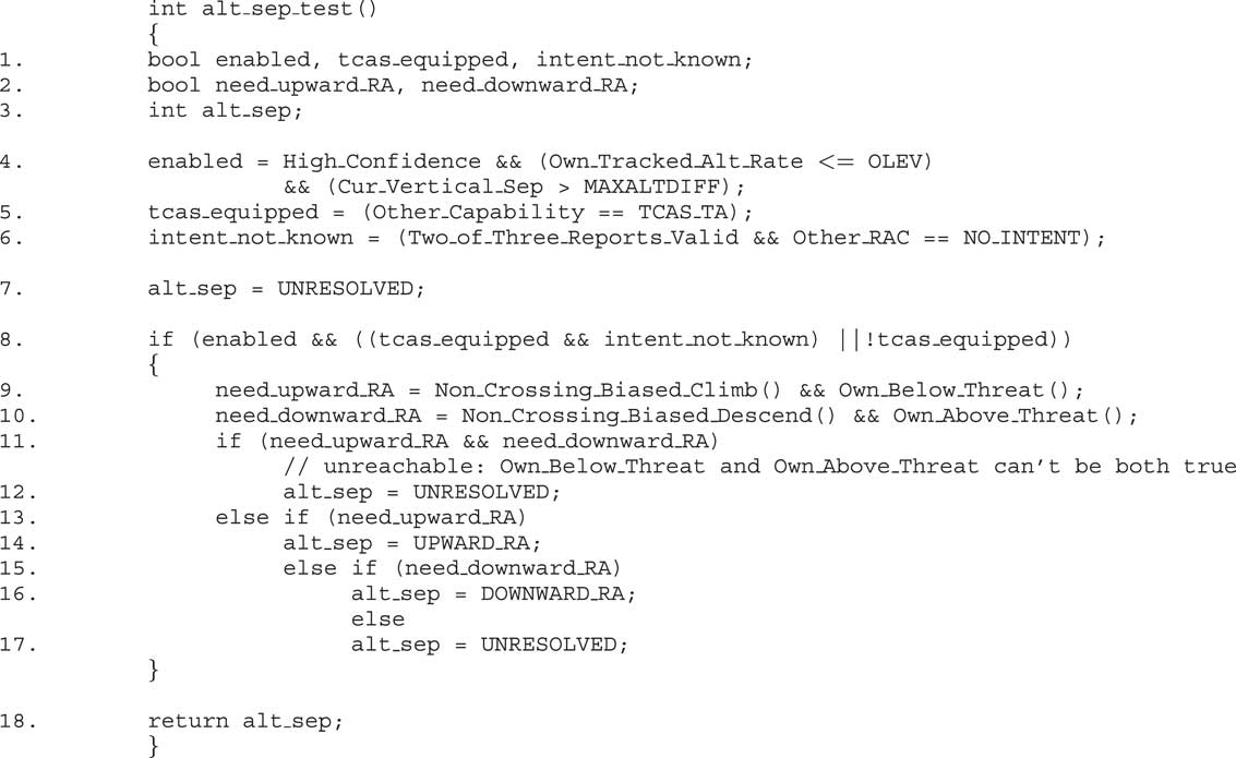
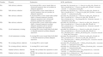
There are many implementations of TCAS, but obtaining the source code of these proprietary implementations is not easy. From the Software-artifact Infrastructure Repository (Do et al., Reference Do, Elbaum and Rothermel2005), it is possible to download a C component, called tcas.c, of a preliminary version of TCAS. This freely and publicly available component is responsible for the RAs issuance. The component is (modestly) made up of 173 lines of C code. The code contains nested conditionals, logical operators, type definitions, macros and function calls, but no floating-point variables, pointers or dynamically allocated structures. Figure 2 shows the call graph of the program while Figure 3 shows the code of the highest-level function Alt_sep_test, which computes the RAs. This function takes 14 global variables as input, including Own_Tracked_Alt the altitude of the TCAS equipped airplane, Other_Tracked_Alt the altitude of the ‘threat’, Positive_RA_Alt_Thresh an adequate separation threshold, Up_Separation the estimated separation altitude resulting from an upward maneuver and Down_Separation the estimated separation altitude resulting from a downward maneuver. The documentation associated to this code indicates that lines 11–12 of Figure 3 is non-executableFootnote 4, showing that this implementation is indeed not compliant with DO-178B. Any TCAS implementation must verify safety properties that come from the aircraft anti-collision theory, as presented in the TCAS II version 7 manual (TCAS II). For the considered component, several properties referring to the possibility of issuing either an upward or a downward RA have been previously formalized in Livadas et al. (Reference Livadas, Lygeros and Lynch1999) and Coen-Porisini et al. (Reference Coen-Porisini, Denaro, Ghezzi and Pezze2001). Table 1 shows the five double properties formalized in (Coen-Porisini et al., Reference Coen-Porisini, Denaro, Ghezzi and Pezze2001). For example, property P1b says that if an upward maneuver does not produce an adequate separation while an downward maneuver does, such as in Figure 4, then an upward RA should not been produced. These properties, among others, are currently verified through manual code reviews. A challenge in this area is to provide automated dependable tools that generate test data, check the conformance of a given implementation with safety properties and show that any statement of the source code is executable. Several experimental tools based on software model checking or static analysis exist for these tasks, but according to our knowledge, none of them is used in operational context on a regular basis. Most of them are still inefficient to deal with nonlinear constraints resulting from constraint disjunction, variable multiplication, division, large array accesses and updates, pointer aliasing and so on. Moreover, proving that a given statement is indeed executable cannot be easily achieved by standard static analysis, as these analyses compute over-approximations of the program states. On the contrary, automatic test case generation tools can produce test inputs able to activate some selected statements of a program, proving so that they are indeed executable.
Call graph of tcas.c

Function alt_sep_test from tcas.c

Safety properties for tcas.c

RA = Resolution advisories.
Resolution advisories. CPA = closest point of approach; TCAS = Traffic Alert and Collision Avoidance System

3 Constraint generation and solving
Our approach is based on a two-stage process. The former stage, called constraint generation, aims at extracting a constraint program from a given test objective and the program under test. The second stage, called constraint solving, aims at solving the resulting constraint system in order to either generate test data or verify the test objective. Constraint generation is now well-documented and our approach has already been discussed in other papers: Gotlieb et al. (Reference Gotlieb, Botella and Rueher2000) presents a constraint generation approach for imperative programs with integer computations, Botella et al. (Reference Botella, Gotlieb and Michel2006) discusses how to deal with floating-point computations while Gotlieb et al. (Reference Gotlieb, Denmat and Botella2007) explains how pointer aliasing can be tackled. On the contrary, the constraint solving stage that relies on constraint propagation, LP and linear relaxations and labeling has been hardly documented. As this paper focusses mainly on constraint solving (Section 3.3), we just briefly recall constraint generation (Section 3.2) after having presented the scope and the notations of our approach (Section 3.1).
3.1 Scope and notations
In this paper, we restrict our presentation to the fragment of the C language required to implement critical sections of programs. The TCAS implementation of our case study is made of arithmetical and logical operations over bounded integers, conditionals and function calls, but there are no loopsFootnote 5, arrays or pointers. Hence, in this paper we confine our presentation to a small subset of the C language, although the approach can deal with unbounded loops (Denmat et al., Reference Denmat, Gotlieb and Ducasse2007a) and other constructions (Gotlieb, Reference Gotlieb2009).
In the rest of the paper, variables of the program under test are noted with lower-case letters while logicial variables are noted with upper-case letters. Any logical variable X is a FD variable with ![\[--><$> \underline{X} <$><[[](https://static.cambridge.org/binary/version/id/urn:cambridge.org:id:binary:20151128095935283-0214:S0269888912000252_eqnU1.gif?pub-status=live) denotating the lower bound of its domain while
![\[--><$> \overline{X} <$><[[](https://static.cambridge.org/binary/version/id/urn:cambridge.org:id:binary:20151128095935283-0214:S0269888912000252_eqnU2.gif?pub-status=live) denotating its upper bound. Arithmetical constraints include constraints built over logical variables and operators such as +, −, *, /, mod, etc. while high-level constraints include conditional constraints (noted c 1→c 2), constraints that handle disjunctions and function calls. Note that c 1→c 2 denotes only half of a logical implication (e.g. ¬c 2→¬c 1 is not a logical deduction of this constraint).
3.2 Constraint generation
3.2.1 Principle
The idea is based on the generation of a constraint program that represents the whole program under test and the test objective. Although other approaches explore one by one each source-code path (Clarke et al., Reference Clarke and Kroening2003; Chaki et al., Reference Chaki, Clarke, Groce, Jha and Veith2004; Godefroid et al., Reference Godefroid, Klarlund and Sen2005; Sen et al., Reference Sen, Marinov and Agha2005; Williams et al., Reference Williams, Marre, Mouy and Roger2005), we choose to explore dynamically all the possible alternatives of the program under test during constraint solving. For example, for each conditional of the program, there are two possible subpaths depending on whether the decision of the conditional is true or not. In standard constraint generation approaches, a choice is made and one of the two subpaths is explored. If this yields a contradiction, the process backtracks until a satisfactory path is found. Contradictions come from path infeasibility: a path is infeasible if and only if the decisions that govern its execution are unsatisfiable. It is worth noticing that programs that contain n conditionals have O(2n) source-code paths in the worst case, among which some may be infeasible, and then standard depth-first search approaches face a combinatorial explosion problem. To leverage this problem, our constraint generation approach implements constraint-based exploration, meaning that each conditional is considered as a constraint that may suspend when there is no subpath alternative to privilege. Instead of using choice points to represent conditionals, our approach keeps implicit disjunctions under the form of specific conditional constraint operators that apply deduction rules to determine whether each disjunct is compatible with the rest of the constraints or not. The constraint model we build represents the whole program under test and when it is considered for constraint solving, it generates a disjunctive constraint system.
3.2.2 Example
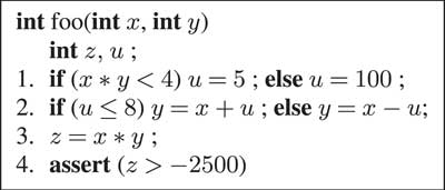
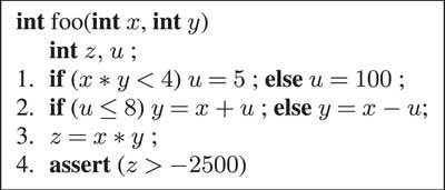
To illustrate this generation, we show the constraint generation stage on the simple example program shown in Figure 5. The program takes two 32-bit signed integer variables as inputs and defines two local variables z and u. At line 4, an assertion checks the value of z. Suppose we want to automatically verify the test objective, which consists of verifying this assertion, that is to check that any state that reaches this assertion admit a value of z strictly >−2500. In this example, the assertion may be invalidated as there exists a test input (values for x and y) that can produce a state where z = −2500 (see Section 3.3.7). The constraint generation step of our method produces the following conditional constraint system, where ite stands for if-then-else: ![\[--><$> X,Y \in \,{\rm{ - }}{{2}^{31}} {{.\,.2}^{31}} \,{\rm{ - }}\,1,<$><[[](https://static.cambridge.org/binary/version/id/urn:cambridge.org:id:binary:20151128095935283-0214:S0269888912000252_eqnU3.gif?pub-status=live)
![\[--><$>Z = \,0,U = 0,\;ite\,(X \,\ast\, Y \lt 4,{{U}_1} = \,5,\,{{U}_1} = 100), \,ite\,({{U}_1} \leq \,8,{{Y}_1} = X + {{U}_1},{{Y}_1} =X{\rm{ - }}\,{{U}_1}),\,{{Z}_1}\, =<$><[[](https://static.cambridge.org/binary/version/id/urn:cambridge.org:id:binary:20151128095935283-0214:S0269888912000252_eqnU4.gif?pub-status=live)
![\[--><$>X \,\ast\, {{Y}_1},{{Z}_1}\leq {\rm{ - }}\,2500 <$><[[](https://static.cambridge.org/binary/version/id/urn:cambridge.org:id:binary:20151128095935283-0214:S0269888912000252_eqnU5.gif?pub-status=live) . This generation uses a renaming scheme, called Static Single Assignment (SSA), to tackle the problem of destructive assignment (Brandis et al., Reference Brandis and Mössenböck1994). When the same variable x is assigned twice in the tested program, two logical instances of the variable X 1 and X 2 are created to properly handle this situation in the constraint program (see Gotlieb et al., Reference Gotlieb, Denmat and Botella2007 for details).
Program foo
3.2.3 Test objectives
As said before, test objectives represent target assertions to verify in the code. Formally speaking, if SC is the constraint system representing the whole program under test and C is an assertion to check, then searching solutions of SC∧¬C answers this verification problem. If one gets that sol(SC∧¬C) = ∅ then assertion C is verified as it holds for any executions of the program. On the contrary, if one gets a solution s then s can be converted into a test input that violates the assertion C. The easiest way to introduce test objectives in the constraint system is therefore, (1) to constrain the execution flow in the program for reaching the assertion and (2) to falsify the assertion in order to find counter-example or to prove it. These goals are handled through a bi-directional process called reification, which constrains the truth value of a given constraint. For example, R ⇔ X > Y associates the reification variable R to the truth value of constraint X > Y. By constraining R, one can specify whether the constraint has to be truth or false. On the contrary, if all the values of domains for X and Y satisfy X > Y (resp. X ⩽ Y) then R = 1 (resp. R = 0). Thanks to this process, the control flow of the program is represented with a boolean constraint network over reification variables. When conditionals are nested, implication between the reification variables of the associated decisions represents the control flow (Gotlieb, Reference Gotlieb2009). Accordingly, assertions are reified and violating an assertion is easily specified by setting its reification variable to 0.
3.3 Constraint solving
Our constraint solving procedure is based on the cooperation of several techniques, namely constraint propagation with bound consistency, LP and linear relaxation and labeling. Each of these techniques has been abundantly described in the literature (Handbook of Constraint Programming, Reference Rossi, van Beek and Walsh2006) and then we focus on the combination of these techniques to validate the TCAS implementation. The constraint solver cooperation is documented in Section 3.3.1, whereas Sections 3.3.2–3.3.6 present linear relaxations of several standard operators. Finally, Section 3.3.7 presents our approach to explore the search space.
3.3.1 The cooperation process
Our constraint solving procedure uses a main propagation queue that manages each constraint in turn. There are two priority levels that can be associated to a constraint. The highest priority level is given to the arithmetical constraints that can prune very early and efficiently the search space. High-level constraints such as conditionals or function calls are tackled with the lowest priority level as they implement costly entailment checks. Our implementation uses a synchronous communication process between two dedicated solvers: a FD constraint propagation solver (FD solver) and a simplex over the rationals (LP solver). Each time an arithmetical constraint is encountered in the propagation queue, two constraints are posted: the arithmetical constraint itself is posted in the FD solver and a linear relaxation over rationals of the arithmetical constraint is posted in the LP solver. This relaxation is computed by using current bounds of domains and then it is called a dynamic linear relaxation (DLR) to underline its iterative computation during the constraint solving process. We explain below with more details how these relaxations can be computed. Each variable of the original problem comes in two flavors: a FD variable for the FD solver and a rational variable for the LP solver. For example, an integer type declaration such as int x yields a domain constraint in the FD solver ![\[--><$> {{X}_{FD}}\, \in \,{\rm{ - }}{{2}^{31}} {{.\,.2}^{31}} {\rm{ - }}1 <$><[[](https://static.cambridge.org/binary/version/id/urn:cambridge.org:id:binary:20151128095935283-0214:S0269888912000252_eqnU6.gif?pub-status=live) and a linear constraint in the LP solver
![\[--><$> {\rm{ - }}{{2}^{31}} \!\leq{{X}_Q}\leq{{2}^{31}} \,{\rm{ - }}1 <$><[[](https://static.cambridge.org/binary/version/id/urn:cambridge.org:id:binary:20151128095935283-0214:S0269888912000252_eqnU7.gif?pub-status=live) where XFD denotes an integer variable and XQ denotes a rational variable.
We selected an LP implementation over the rationals in order to preserve correctness. Using a more efficient implementation based on floating-point computations would have been desirable, but our goal is to preserve the semantics of integer computations, and floating-point computations in LP are sometimes unsafe to preserve all the real solutions. In the conclusion section of the paper, we discuss the possible use of safe LP implementations, such as (Neumaier et al., Reference Neumaier and Shcherbina2004), to preserve the semantics. Therefore, having relaxed the constraint system over integer variables into a linear problem over rationals permits to check for satisfiability with more efficiency. Indeed, the LP solver considers the constraint system as a whole while the FD solver checks for satisfiability by combining only local tests of each constraint.
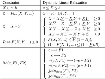
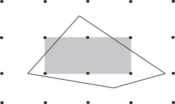
Note also that some nonlinear constraints over integers can be handled with relaxations. We provide in Figure 6 the formulas we used for relaxing constraints having variable multiplication, reification, conditionals, etc. Several strategies can be followed to make both solvers cooperate. We tried several heuristics and kept the one that gave the best results in average. The idea is to call each solver in turn (without interleaving) to benefit from their combined efficiency. Starting with the FD solver, a constraint propagation step with bound-filtering consistency is launched. Upon fixpoint, the DLRs are then computed using the current bounds of variable and the LP solver is called by optimizing the bounds of each variable. When the relaxed linear problem does not contain any solutions, it means that the original (possibly nonlinear) problem is unsatisfiable. This property comes from the fact that correctness was preserved by the use of relaxations over rationals. On the contrary, when the relaxed linear problem contains solutions, one can still benefit from the simplex to prune the variation domains of variables. The idea is to project the current polyhedron over each variable and comparing the resulting domain with the current domain of variable. This algorithm performs two calls to the simplex algorithm per variable appearing in the linear relaxation, one call for each bound. Then, it prunes the current domain of variable by updating its (rational) bounds. Finally, integer rounding shaves the domain to fit with integer solutions only. For example, if a call to the simplex returns 7/2 as an upper bound for X, then variable X has to be lower or equal to 3. As a result, the constraint solving process computes an integer bounding box that includes all the integer solutions of the linear relaxed problem. Note, however, that the box may also include integer points that are no part of the polyhedron, as shown in Figure 7. Pruning the domain of variables awakes FD constraints still suspended and constraint propagation can be re-launched to get better over-approximation. This iterating process is repeated until a fixpoint is reached for both solvers. At this point, a labeling procedure is launched that can possibly awake constraint propagation and DLRs computations.
Dynamic linear relaxations (DLRs)

The grey box contains all the integer points inside the polyhedron

A drawback of this approach is the possible slow convergence of the iterating process. However, any approach that makes at least two solvers cooperate faces a similar problem. In practice, we did not observe any slow convergence phenomenon in our experiments until now.
3.3.2 Dynamic linear relaxation of multiplication
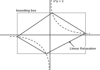
The formula of Figure 6 for multiplication directly follows from the four following trivial inequalities (McCormick, Reference McCormick1976):

Figure 8 shows a slice of the relaxation where Z = 1. Here, the rectangle corresponds to the bounding box of variables X and Y, the dashed curve represents exactly X * Y = 1, while the four solid lines correspond to the inequalities of the relaxation.
Relaxation of multiplication

3.3.3 Dynamic linear relaxation of division, modulo and logical operators
Expressions built on division and modulo can be treated with similar linear relaxation reformulation. The constraint Q = A div B where div denotes the Euclidian division rewrites to

Similarly, R = A mod B where mod denotes the Euclidian remainder rewrites to

We applied the same principle for logical operators by studying the semantics of operators of the C programming language. The constraint Z = X && Y, where && denotes the ‘logical and’ operator rewrites to

The constraint Z = X∥Y, where ∥ denotes ‘logical or’ rewrites to

while Y = ∼X, where ∼ denotes ‘logical not’ rewritesFootnote 6 to

3.3.4 Handling reification
Reified constraints appear in the constraint system as the result of control flow specification (reaching a specific location) or assertion violation. Consider the reified constraint R ⇔ C, where R is the reification variable. Without any loss of generality, let suppose that C is of the form F(X) ⩽ 0 and the function F is bounded, that is there exist ![\[--><$> \underline{F} <$><[[](https://static.cambridge.org/binary/version/id/urn:cambridge.org:id:binary:20151128095935283-0214:S0269888912000252_eqnU14.gif?pub-status=live) and
![\[--><$> \overline{F} <$><[[](https://static.cambridge.org/binary/version/id/urn:cambridge.org:id:binary:20151128095935283-0214:S0269888912000252_eqnU15.gif?pub-status=live) such that
![\[--><$> \forall X \in {{D}_X} \underline{F} \,\leqslant\,F(X)\,\leqslant\,\overline{F} <$><[[](https://static.cambridge.org/binary/version/id/urn:cambridge.org:id:binary:20151128095935283-0214:S0269888912000252_eqnU16.gif?pub-status=live) . Then R ⇔ F(X) ⩽ 0 rewrites to the conjunction

For example, consider the constraint R ⇔ X ⩽ Y, then ![\[--><$> F(X,Y)\, = \,X\,{\rm{ - }}\,Y,\;\underline{F} \, = \,\underline{{X\,}} {\rm{ - }}\,\overline{Y}, \;<$><[[](https://static.cambridge.org/binary/version/id/urn:cambridge.org:id:binary:20151128095935283-0214:S0269888912000252_eqnU18.gif?pub-status=live)
![\[--><$>\overline{F} \, = \,\overline{X} \,{\rm{ - }}\,\underline{Y} <$><[[](https://static.cambridge.org/binary/version/id/urn:cambridge.org:id:binary:20151128095935283-0214:S0269888912000252_eqnU19.gif?pub-status=live) , and the reified constraint rewrites to

Note that these inequations are interpreted over the rationals. Hence, the boolean variable R is interpreted as a rational over the continuous set [0,1] and then the set of solutions of these constraints (over-) approximates only the solutions over integers.
3.3.5 Handling conditionals
We use a special operator called ite for handling conditionals. This operator is implemented as a global constraint, meaning that it can be awoken when the variation domain of at least one of its variables changes. Once awoken, the algorithm of this constraint tries to prove that one of the two disjuncts is unsatisfiable with the rest of the constraints and, thus, replaces the overall disjunction by the other disjunct. When this reasoning fails, the union of domains is computed.
Constraint ite is modeled using four guarded constraints. The former two directly come from the operational semantics of a conditional in a C program: c→F1,¬c→F2. They are used to propagate forward control flow throughout the constraint system. On the contrary, the latter two implement backward reasoning: ![\[--><$> \neg (c \wedge F1)\, \rightarrow \,(\neg c \wedge F2) <$><[[](https://static.cambridge.org/binary/version/id/urn:cambridge.org:id:binary:20151128095935283-0214:S0269888912000252_eqnU21.gif?pub-status=live) and
![\[--><$> \neg (\neg c \wedge F2)\, \rightarrow \,(c \wedge F1) <$><[[](https://static.cambridge.org/binary/version/id/urn:cambridge.org:id:binary:20151128095935283-0214:S0269888912000252_eqnU22.gif?pub-status=live) . Roughly speaking, ite represents exclusive disjunction between two disjuncts and these four guarded constraints come from this declarative view. It is worth noticing that the key behind guarded constraint implementation is constraint entailment. A constraint entailment test permits to evaluate the guard and it can be implemented by adding the negation of the guard to the rest of the constraint store and check whether the resulting system is unsatisfiable. When the system is still satisfiable (or at least partially consistent), the negated constraint must be removed from the store and other constraint entailment tests can be performed. Note also that other ite or function call operators can be nested in a given guarded constraint. To alleviate the potential combinatorial explosion of constraint entailment checks, we set up a bound on the depth of search within the guards. For example, if the bound is set to 1, then no other ite or function calls operators of F2 will be unfolded when the guard
![\[--><$> \neg c \wedge F2 <$><[[](https://static.cambridge.org/binary/version/id/urn:cambridge.org:id:binary:20151128095935283-0214:S0269888912000252_eqnU23.gif?pub-status=live) is explored. In practice, we set up the bound to 2, meaning that every couple of conditionals of the program were explored for finding inconsistencies and then to prune the search space. When both cases within an ite are explored without success, then two join operators are posted: a join operator on FDs to merge the results for each FD variable, and a join on polyhedra.
In the example of Figure 5, suppose for the sake of clarity that the domains of each variable are initailly restricted to −1000..1000. From the first conditional constraint ![\[--><$>ite(X \ast Y\, \leqslant \,4,{{U}_1}\, = \,5,{{U}_1}\, = \,100)<$><[[](https://static.cambridge.org/binary/version/id/urn:cambridge.org:id:binary:20151128095935283-0214:S0269888912000252_eqnU24.gif?pub-status=live) , we get that the domain of U 1 is trivially pruned to 5..100. From the second conditional constraint
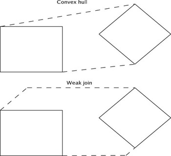
![\[--><$>ite({{U}_1} \leqslant 8,{{Y}_1}\, = \,X\, + \,{{U}_1},{{Y}_1}\, = \,X\,{\rm{ - }}\,{{U}_1})<$><[[](https://static.cambridge.org/binary/version/id/urn:cambridge.org:id:binary:20151128095935283-0214:S0269888912000252_eqnU25.gif?pub-status=live) , the domain of X in the then-part is pruned to −1000..995 and the domain of Y 1 to −995..1000 as U 1 = 5 in this case. In the else-part, the domain of X is pruned to −900..1000 and the domain of Y 1 to −1000..900 as U 1 = 100. Perfoming the domain join on both domains leaves the domains of X and Y 1 unchanged. On the contrary, the polyhedral join offers more precise results. From the second conditional, we get that −100 ⩽ Y 1 − X ⩽ 5. The smallest and then more desirable linear relaxation of the union of of two subsets of linear inequations is the the convex hull of the two corresponding polyhedra. Unfortunately, computing the convex hull of two polyhedra (when they are given under the form of inequations) is exponential in the number of dimensions. By noticing that any over-approximation of the convex hull is suitable in our context, we proposed in Denmat et al. (Reference Denmat, Gotlieb and Ducasse2007b) to use the weak-join operator, originally proposed in the Abstract Interpretation community (Sankaranarayanan et al., Reference Sankaranarayanan, Colòn, Sipma and Manna2006). Roughly speaking, the weak join of two sets of inequations consists in (1) enlarging the first polyhedron without changing the slope of the lines until it encloses the second polyhedron; (2) enlarging the second polyhedron in the same way; and (3) returning the intersection of these two new sets of inequations. Figure 9 shows the difference between the convex hull and the weak join of two polyhedra E and F. Formally, let S = E ∪ F be the set of inequations that appear in E or in F. Let suppose that each inequation in S is of the form Ai.X ⩽ bi, where Ai is a vector of n coefficients, X is a vector of n variables and bi is a rational number. For each inequation in S do

Weak Join vs. Convex Hull

maximize(Ai.X,E) denotes a call to the simplex algorithm that computes the maximum value of expression Ai.X under the linear constraints E. Then, ![\[--><$> joi{{n}_{lin}}(E,F)\, = \,{{\{ {{A}_i}.X \leqslant c\} }_{i \in 1.|S|}} <$><[[](https://static.cambridge.org/binary/version/id/urn:cambridge.org:id:binary:20151128095935283-0214:S0269888912000252_eqnU27.gif?pub-status=live) . Based on the simplex, this algorithm performs well in practice.
3.3.6 Handling function calls
In the TCAS implementation, dealing efficiently with functions is important as there are many function calls, some of them being irrelevant to prove a given safety-critical property. In our framework, function calls are handled with a special operator called rel_call, that can be awoken on domain prunings, as any other constraint. The idea is to use lazy evaluation of function calls by unfolding calls only when necessary. Initially, function calls are simply ignored, and the consistency of the constraint store is evaluated without the constraints of the function calls. If the store is still partially consistent, the constraints issued from one callee are introduced into the propagarion queue and again, the consistency is evaluated. This process is iterated until no more function calls can be considered. This strategy is motivated by our will to minimize the number of constraints used to prove a given assertion. There are many other heuristics to introduce constraints of the callee function, but we did not push this analysis further. We implemented this strategy by a simple breadth first strategy over the call tree of the function under test.
3.3.7 Labeling
As our TCAS problem includes nonlinear constraints over bounded integers, the final step of the resolution process may include a labeling phase to exhibit a solution or prove there is no solution. However, as the number of variables and the variation domain of each variable are both large (TCAS takes 14 global 32-bit variables as input), resorting to enumeration to show unsatisfiability is usually prohibitive. Hence, most of the hard work has to be performed during constraint propagation. Linear relaxation of nonlinear constraint was introduced in our framework to answer this problem, but as it computes over-approximations, there remain cases for which one resorts to labeling. For selecting variable and value to enumerate first, we explored several available heuristics such as first-fail, domain splitting or most-constrained first. We also implemented two other simple labeling heuristics: iterative domain splitting and random labeling. Iterative domain splitting selects a variable X from an (static) input list and a value v in the domain of this variable, makes a non-deterministic choice between X = v, X > v and X < v and iterates over these processes until no more variable remains unassigned. Random labeling does the same except that the value v is chosen at random, using a uniform probability distribution over the domain. Randomization is interesting in the context of test data generation as it introduces uncertainty in the way test data are selected. In average, we found that these two heuristics performed well on the various distinct requests for TCAS. Coming back to the example of Figure 5, using this labeling step, we found that there are counter-examples to the assertion of line 4. For example, (X = 50, Y = 1) is a solution to the (nonlinear) constraint system: ![\[--><$> X,Y \in \,{\rm{ - }}{{2}^{31}} {{.\,.2}^{31}} \,{\rm{ - }}\,1,\;{{U}_1} \in 5.100, <$><[[](https://static.cambridge.org/binary/version/id/urn:cambridge.org:id:binary:20151128095935283-0214:S0269888912000252_eqnU28.gif?pub-status=live)
![\[--><$>ite(X \,\ast\, Y \lt \,4,\,{{U}_1} = \,5,\;{{U}_1} = 100),\;ite({{U}_1} \lt 8,\;{{Y}_1} = X + {{U}_1},\;{{Y}_1} = \,X\,{\rm{ - }}\,{{U}_1}),\;{\rm{ - }}100 \leqslant {{Y}_1}\,{\rm{ - }}\,X \leqslant \hskip 1.4pt 5, <$><[[](https://static.cambridge.org/binary/version/id/urn:cambridge.org:id:binary:20151128095935283-0214:S0269888912000252_eqnU29.gif?pub-status=live)
![\[--><$>{{Z}_1} = \,X \ast {{Y}_1},\;{{Z}_1} \leqslant {\rm{ - }}\,2500 <$><[[](https://static.cambridge.org/binary/version/id/urn:cambridge.org:id:binary:20151128095935283-0214:S0269888912000252_eqnU30.gif?pub-status=live) and then using these values as a test data for program foo yields assertion violation on line 4. It is worth noticing this counter-example has been found without making any choice in the conditionals during initial propagation. Replacing the assertion of line 4 by assert (z > −3000) in the source code of program foo yields ‘fail’ when one tries to find counter-examples, which indicates that the assertion is satisfied by any state.
4 Implementation
The procedure described in this paper has been implemented following the architecture shown in Figure 10. The procedure takes a C file as input, optionally annotated with pre/post-conditions, assertions or reach directives. A directive ‘reach’ specifies a location to reach within the code. Parsing the C file builds an abstract syntax tree and a symbol table. Then, using a normalization and points-to analysis, the syntax tree is transformed into SSA form and then, a constraint intermediate form is produced. From there, constraint solving is launched according to some parameterization through an evaluator component. The solving procedure is based on the combination of two existing solvers through a high-level propagation queue: the clpfd library of SICStus Prolog, which implements FD constraint solving (Carlsson et al., Reference Carlsson, Ottosson and Carlson1997); and the clpq library that implements a LP solver based on Fourier's elimination and simplex over the rationals (Reference Holzbaurclp(q,r) Manual). When a solution is found, it is reported to the user as a test data that satisfies the test objective (reach a given location, violate an assertion or find a counter-example to a post-condition). When the solver outputs ‘fail’, meaning that the constraint system is inconsistent, then this indication is also reported to the user. It indicates that the test objective is unsatisfiable or the assertion is verified.
Implementation

The constraint solving procedure is mainly developed in Prolog (∼10 KLOC) and C (∼0.3 KLOC). The internal components include a backtrackable C parser written with the Definite Clause Grammar of Prolog, a SSA form generator based on the single-pass generation algorithm of Brandis et al. (Reference Brandis and Mössenböck1994), a constraint intermediate form generator and parser, a library of high-level constraints that implements most of the C operations (conditionals, loops, logical operators, function call operator, memory operations,…). To make both constraint solvers cooperate, we exploited the SICStus global constraint interface to define constraints that awakes constraint propagation over FD. One weakness of this approach is that it delegates constraint management to the system and does not allow the order in which the constraints are considered in the queue to be modified easily. Note also that SICStus clpfd combines indistinctly two levels of filtering: domain-consistency and interval-consistency. Moreover, we encountered some limit problems with clpfd as the value of an FD variable is represented on less than 32-bits. Another problem concerns the semantics of integer computations within the constraint solver that does not mimic the semantics of integer computations in a C program, which implements the so-called wrapping effect. In fact, arithmetic operators in C programs implement arithmetic modulo 8, 16, 32 or 64 bits and some programs may use this effect either conscientiously or not. For example, a statement such as z = x + y where x, y, z are 32-bit integers should be interpreted as ![\[--><$> z\, = \,(x\, + \,y)\;mod{{(2}^{32}} ) <$><[[](https://static.cambridge.org/binary/version/id/urn:cambridge.org:id:binary:20151128095935283-0214:S0269888912000252_eqnU31.gif?pub-status=live) . However, using this formulation would have been catastrophic in our context as 32-bit integers cannot be represented in the SICStus FD constraint solverFootnote 7 and bound-consistency on modulo operator is weak in general. As a consequence, our approach implicitly rejects any state of the program that exploits the wrapping effect.
5 Results and analysis
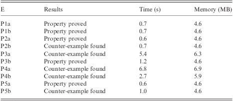
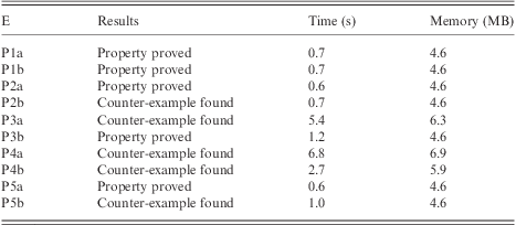
We conducted several experiments on a small software component of the TCAS to evaluate the capabilities of our constraint procedure to serve as an aid for testing and verification. First, we evaluated structural test data generation for the coverage of the all decisions criterion. Covering this criterion is mandatory in the context of a DO-178B B level certification. On an Intel Core Duo 2.4 GHz clocked PC with 2 GB of RAM, Euclide generated a test set covering all the executable decisions of the tcas program in 16.9 seconds, including time spent garbage collecting, stack shifting or in system calls. It also showed that the decision of line 11–12 of Figure 3 was non-executable in less than 0.2 second. Second, we evaluate automatic program verification on the safety properties of Table 1. Results are shown in Table 2.
Verification of safety properties
Finding counter-examples to safety properties is usually dramatic. Hopefully, the software component we used probably corresponds to a preliminary version and it has never been used in operational conditions.
Surprisingly, we found that properties P2B, P3A and P5B were not proved w.r.t. the implementation and counter-examples were exhibited. These counter-examples satisfy the preconditions but they invalidate the post-conditions when they are submitted to the implementation. Therefore, they are realistic counter-examples. All the material of these experiments, including the test data corresponding to counter-examples, is available onlineFootnote 8. We executed the implementation with test data and dynamically checked that properties P2B, P3A and P5B were indeed violated. The counter-examples to properties P5B were not reported in other papers (Coen-Porisini et al., Reference Coen-Porisini, Denaro, Ghezzi and Pezze2001; Clarke et al., Reference Clarke and Kroening2003; Chaki et al., Reference Chaki, Clarke, Groce, Jha and Veith2004). Moreover, these counter-examples and proofs were obtained quickly (all the counter-examples and proofs are generated in less than 20 seconds on our standard machine), which is encouraging for a future comparison with other dedicated tools.
6 Related work
Automatic program verification is a fundamental topic that was recently revamped due to the considerable improvments in SAT- and SMT (SATisfiability Modulo Theories)- solving. Software model checkers such as Save (Coen-Porisini et al., Reference Coen-Porisini, Denaro, Ghezzi and Pezze2001), Blast (Henzinger et al., Reference Henzinger, Jhala, Majumdar and Sutre2003), Magic (Chaki et al., 2003) or Cbmc (Clarke et al., Reference Clarke and Kroening2003) routinely find counter-examples to temporal properties over C programs. These tools explore the paths of a bounded model by decomposing path constraints into SAT-formula. These formula, extracted from C expressions, are checked for satisfiability or unsatisfiability (Brummayer et al., Reference Brummayer and Biere2007). Some of them also exploit predicate abstraction and counter-example refinement to boost the exploration. Our constraint solving contrasts with SAT-based or SMT-based model checkers as it does not abstract the program and does not generate spurious counter-example paths. In particular, it builds a high-level constraint model of C program by capturing error-free semantics without considering a boolean abstraction of the program structure. In addition, our approach exploit LP relaxations to solve nonlinear constraint systems, something which is currently outside the scope of SMT-solvers. Building a constraint solving procedure that makes an FD solver and an LP solver cooperate is not new. In 1995, Beringer and De Backer proposed a global constraint that captures the linear constraints of the problem. This approach was generalized in Milano et al. (Reference Milano, Ottosson, Refalo and Thorsteinsson2002) and Hooker et al. (Reference Hooker, Erlender, Thorsteinsson and Kim2000). Linear relaxations of nonlinear constraints is also an old idea that dates back to the 1970s (McCormick, Reference McCormick1976; Balas, Reference Balas1985) and has been extended to CP by Refalo with the idea of ‘tight cooperation’ (Refalo, Reference Refalo1999). Recently, Lebbah et al. (Reference Lebbah, Michel and Rueher2005) proposed to use similar principles to deal with quadratic constraints over continuous domains. Although there are some similarities, our constraint solving approach distinguishes because it addresses specifically disjunctive nonlinear constraint systems over bounded integers and preserves the correctness of results even when relaxing nonlinear constraint. Our approach has also similarities with the Collavizza and Rueher (Collavizza et al., Reference Collavizza and Rueher2006) approach that calls several constraint solvers in sequence. Recently, they showed that their Cpbpv implementation could outperform usual software model checkers on classical benchmarks (Collavizza et al., Reference Collavizza, Rueher and Van Hentenryck2008). Cpbpv is based on deductive CP techniques that statically combines SAT solving, LP and constraint propagation. However, more experimental work still need to be performed to confirm these results, obtained on a restricted subset of academic programs. According to our knowledge, our application of rational linear relaxations to software verification is original.
Automatic test data generation based on constraint propagation has been early explored in Bicevskis et al. (Reference Bicevskis, Borzovs, Straujums, Zarins and Miller1979), DeMillo et al. (Reference DeMillo and Offut1991) and Offut et al. (Reference Offut, Jin and Pan1999). In this latter work, the dynamic domain reduction procedure that implements constraint propagation with bound-consistency was proposed. PathCrawler (Williams et al., Reference Williams, Marre, Mouy and Roger2005) is a recent path-oriented structural test data generator based on FD constraint solving. It exploits the constraint library Colibri developed by Bruno Marre that implements several powerful pruning techniques such as difference logics and congruence relations in addition to bound-filtering. Dart (Godefroid et al., Reference Godefroid, Klarlund and Sen2005) and CUTE (Sen, Reference Sen, Marinov and Agha2005) are two other popular path-oriented test data generators based on LP over floating-point variables (lpsolve) and concrete execution. Unlike these approaches, our constraint solving procedure preserves correctness by using LP over rationals. It may be less efficient, but preserving correctness is essential in a context where properties over programs must be verified and not only tested.
7 Conclusion
In this paper, we presented a constraint solving procedure dedicated to the verification of safety-critical properties of C programs. As a first validation step, our solver was used on a freely available software component extracted from a real application (TCAS), for which safety-critical properties have been defined. It found that a complete test set covering all the executable decisions of the program could be obtained in less than 20 seconds of runtime. Our approach could also prove that some of the safety-critical properties were satisfied, whereas other were invalidated in a few seconds. Hence, these preliminary results show that using CP techniques for property verification is viable and efficient. However, both foundational and applied research works still need to be undertaken in order to address more realistic implementations that contain hundreds of thousand lines of code. Methods to integrate new verification tools in the development chain should also be proposed. In our framework, we exploited an existing FD solver that manages its own propagation queue and implements its own filtering algorithms. We forecast the development of a dedicated FD solver based on bound-consistency filtering that could be used to check real-sized integer computations. Modeling accurately the wrapping effect would permit to find bugs related to integer representation, which is outside the scope of current test data generators. Another line of research concerns the integration of a safe LP implementation over floating-point computations (Neumaier et al., Reference Neumaier and Shcherbina2004) instead of using less efficient implementation over rationals. As preserving correctness is essential when one wants to prove safety properties, this requires safe over-approximations of the solution set to be computed.
Acknowledgments
I am very grateful to Tristan Denmat who investigated the role of Abstract Interpretation in the ideas presented here. In particular, he provided us with the weak-join idea that comes from this community. Many thanks to David Delmas from Airbus Industries and the anonymous referees for their careful reading of the preliminary versions of the paper.