1 Introduction
In real-world applications, large-scale systems are difficult to optimally configure, often because communication restrictions, organizational structures and/or complicated topologies make it difficult, costly, or impossible to collect all the necessary information at a location where a solution can be computed. This, in turn, motivates the use of distributed methods of optimization in order to find the optimal configuration. In particular, in this paper, we concentrate on multi-agent systems—that is, systems in which control is distributed across a set of autonomous agents—as an important approach to distributed optimization. Within this context, we focus specifically on distributed constraint optimization problems (DCOPs), a broad family of problems that can be brought to bear on many domains, including: disaster response scenarios (e.g. Kitano et al., Reference Kitano, Todokoro, Noda, Matsubara, Takahashi, Shinjou and Shimada1999; Chapman et al., Reference Chapman, Micillo, Kota and Jennings2009), wide-area surveillance and distributed sensor network management (e.g. Hayajneh & Abdallah, Reference Hayajneh and Abdallah2004; Heikkinen, Reference Heikkinen2006; Kho et al., Reference Kho, Rogers and Jennings2009), industrial task allocation and scheduling problems (e.g. Zhang & Xing, Reference Zhang and Xing2002; Stranjak et al., Reference Stranjak, Dutta, Ebden, Rogers and Vytelingum2008), and the management of congested air, road, rail, and information networks (e.g. van Leeuwen et al., Reference van Leeuwen, Hesselink and Rohling2002; Roughgarden, Reference Roughgarden2005).
In more detail, in a constraint satisfaction problem, the aim is to find a configuration of states of variables such that they satisfy a set of constraints. A constraint optimization problem is then given by a utility function that aggregates the payoffs for satisfying each of a set of ‘soft’ constraints (or, conversely, a penalty for violating constraints) over the states of variables in the problem (Schiex et al., Reference Schiex, Fargier and Verfaillie1995). A distributed constraint optimisation problem arises when a number of independent agents each control the state of (a subset of) the variables in the system, with the joint aim of maximizing the global reward for satisfying constraints. A natural way to model DCOPs, then, is as a multi-agent system.
As a consequence of the breadth of applications of DCOPs, many algorithms for solving them have been developed using a number of approaches, which often differ according to the literatures they were first proposed in (e.g. the computer science, game theory, machine learning, or statistical physics literatures). It is our intention, then, to provide a unifying framework for analyzing a broad class of DCOP algorithms. However, here we exclude from our analysis centralized approaches in which all of the information needed to solve the DCOP is directly accessible to, and/or in which all of the variables in a system come under the control of, a single decision maker, as assumed within algorithms such as the breakout algorithm (Morris, Reference Morris1993) and arc consistency (Cooper et al., Reference Cooper, de Givry and Schiex2007), among others (see Apt (Reference Apt2003), for more examples from the broader constraint programming literature). While such approaches are certainly useful in a range of scenarios, we make this exclusion because we are particularly interested in algorithms for multi-agent systems, in which the actors are distributed and can only communicate with their peers. The remaining algorithms are known as distributed algorithms, and, for our purposes, we define three further sub-groupings:
• Distributed complete algorithms, by which we mean algorithms that always find a configuration of variables that maximizes the global objective function (as in finite domains one always exists). This class includes ADOPT (Asynchronous Distributed OPTimization; Modi et al., Reference Modi, Shen, Tambe and Yokoo2005), DPOP (Dynamic Programming OPtimization; Petcu and Faltings, Reference Petcu and Faltings2005), and APO (Asynchronous Partial Overlay; Mailler and Lesser, Reference Mailler and Lesser2006). Due to the inherent computational complexity of DCOPs, complete algorithms always run exponential in some aspect of their operation (i.e. the number or size of messages exchanged, or the computation performed by the agents). Furthermore, distributed complete algorithms usually operate by passing complicated data structures, or run on a highly structured ordering, such as a spanning tree, and often require additional processing of the original constraint graph.
• Local iterative message-passing algorithms, such as max-sum (Aji & McEliece, Reference Aji and McEliece2000) or distributed arc consistency (Cooper et al., Reference Cooper, de Givry and Schiex2007). In these algorithms, neighbouring agents exchange messages comprising a data structure that contains the values of different local variable configurations, and use these values to construct new messages to pass on to other agents.
• Local iterative approximate best-response algorithms, such as the distributed stochastic algorithm (Tel, Reference Tel2000; Fitzpatrick & Meertens, Reference Fitzpatrick and Meertens2003), the maximum-gain messaging algorithm (Yokoo & Hirayama, Reference Yokoo and Hirayama1996; Maheswaran et al., Reference Maheswaran, Pearce and Tambe2005), fictitious play (Brown, Reference Brown1951; Robinson, Reference Robinson1951), adaptive play (Young, Reference Young1993, Reference Young1998), and regret matching (Hart & Mas-Colell, Reference Hart and Mas-Colell2000). In this class, agents exchange messages containing only their state, or can observe the strategies of their neighbours. In game-theoretic parlance, this is known as standard monitoring Footnote 2, and, as the name suggests, is a typical informational assumption implicit in the literature on learning in games.
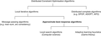
In this paper, we refer to the last two groups together as local iterative algorithms (see the taxonomy in Figure 1), to differentiate them from their complete counterpartsFootnote 3. We group them under this term because both classes operate only at the local level, with messages exchanged between neighbouring agents at each iteration of the algorithm, and without any overarching structure controlling the timing or ordering of messages.
Taxonomy of the categories of algorithms considered in this paper, with the focus, local iterative approximate best-response algorithms, in bold.

In many real distributed systems, we find that local iterative algorithms are often preferred over distributed complete algorithmsFootnote 4. This is because, in such domains, it is necessary and appropriate to trade solution quality off against timeliness or communication overhead. For example, in real-time target tracking it may be more important to produce a good solution quickly, rather than wait for the optimal solution. This is the reasoning Krainin et al. (Reference Krainin, An and Lesser2007) invoke to motivate their use of the local iterative algorithm to coordinate scan schedules in a real meteorological radar network. Similarly, in remote and mobile sensor management, an algorithm that has a low communication overhead may be preferred because of the large drain on a sensor's battery charge caused by communication, as evidenced by the choice of algorithm used in many problems in distributed sensor networks (e.g. Zhang et al., Reference Zhang, Wang, Xing and Wittenburg2005; Farinelli et al., Reference Farinelli, Rogers, Petcu and Jennings2008) and multi-robot cooperative data fusion problems (e.g. Matthews & Durrant-Whyte, Reference Matthews and Durrant-Whyte2006; Stranders et al., Reference Stranders, Farinelli, Rogers and Jennings2009). Furthermore, in some real distributed systems, hardware limitations may outright prohibit the use of distributed complete algorithms. For example, when using DPOP the capacity of the communication buffer of a typical sensor node is quickly exceeded as a problem grows in size, because the message size is exponential in the induced width of the communication tree (e.g. Petcu & Faltings, Reference Petcu and Faltings2005; Rogers et al., Reference Rogers, Corkill and Jennings2009). Similarly, the number of messages exchanged in ADOPT is exponential in the height of the communication tree, and in APO, the mediator agents are required to perform computations, which grow exponentially in the size of the portion of the problem they are responsible for. Such exponential relationships are simply unacceptable in embedded devices that exhibit constrained computation, bandwidth, and memory resources. On the other hand, in these settings, it is clear that local algorithms are more effective, because the quality of the solutions they produce are typically satisfactory (even if they are not optimal), and they perform favourably in terms of the issues of scalability mentioned above.
Now, the characteristics of complete DCOP algorithms are well understood, and the properties of the entire framework of local message-passing algorithms have been extensively analyzed, with guarantees placed on their solutions under a range of assumptions, for example, for tree structured (Aji & McEliece, Reference Aji and McEliece2000) or single-looped constraint graphs (Weiss, Reference Weiss2000). In contrast, no such unifying and categorizing framework has existed for local iterative algorithms until now. One reason for this is because, broadly speaking, these algorithms originate from two different literatures; either they are learning or adaptive processes taken from game theory or they are distributed versions of centralized procedures developed for traditional constraint optimization problems or heuristic search methods taken from computer science. In more detail (centralized), constraint optimization problems evolved, in part, as a method for analyzing over-constrained constraint satisfaction problems. As such, traditional computer science approaches to such problems include the breakout algorithm, arc consistency, dynamic programming, and stochastic optimization techniques. Consequently, a traditional computer science approach to solving DCOPs, which includes many local approximate best-response algorithms, starts by developing distributed versions of these centralized algorithms. For example, distributed breakout (Hirayama & Yokoo, Reference Hirayama and Yokoo2005) and maximum-gain messaging (Maheswaran et al., Reference Maheswaran, Pearce and Tambe2005) are two local approximate best-response algorithms that descend from the breakout algorithm, and distributed versions of simulated annealing have been developed for DCOPs (Fitzpatrick & Meertens, Reference Fitzpatrick and Meertens2003; Arshad & Silaghi, Reference Arshad and Silaghi2003), which also fall into the category of local approximate best-response algorithms. On the other hand, from a game-theoretic perspective, in a DCOP, each autonomous agent's aim is to maximize its own private utility function through its independent choice of state. From this point of view, each agent's optimal choice is strategically dependent on the actions of its neighbouring agents (a perspective on DCOPs first adopted by Maheswaran et al., Reference Maheswaran, Pearce and Tambe2004), and distributed algorithms for solving such problems is the focus of the literature of learning in games (e.g. Fudenberg & Levine, Reference Fudenberg and Levine1998). However, what is common to both of these literatures is that the techniques used are all local, iterative, approximate best-response algorithms, in which agents exchange messages containing only their state, and which typically converge to local optima (or Nash equilibria); and it is game theory that has the tools and terminology to analyze algorithms that operate in such settings. In particular, we stress that, in giving up global optimality, we consider the set of local optima, or equivalently, Nash equilibria, to be the appropriate solution concept for this class of algorithm. This is because this set represents the stable configurations of variables that can be reached by exchanging messages that contain only an agent's state (i.e. the information in the messages circulated in all of the algorithms in this class defines the appropriate solution concept).
Against this background, the main contribution of this paper is the first unifying analytical framework for studying iterative approximate best-response algorithms that are used to solve both DCOPs and potential games. Our framework is based on a problem formulation known as a hypergraphical game (Papadimitriou & Roughgarden, Reference Papadimitriou and Roughgarden2008) and convergence results regarding the class of potential games (Monderer & Shapley, Reference Monderer and Shapley1996b). Specifically, we show that a hypergraphical game is a potential game if every local interaction can be represented as a local potential game, and this is the case for all DCOPs. We then use this framework to develop a novel parameterization of iterative approximate best-response DCOP algorithms. In order to populate this parameterization, we decompose algorithms proposed in both the game theory and computer science literatures in such a way so as to identify categories of substitutable components. We then analyze how these components affect the convergence properties of an algorithm employing them, using convergence analysis techniques developed specifically for potential games. As such, our framework can be applied to potential games generally. However, due to the fact that we are considering these algorithms as distributed optimization tools, we restrict the larger part of our discussion to the specific case of DCOP games.
In more detail, in this paper, we advance the state of the art in the following ways:
1. We derive a general result regarding hypergraphical potential games, which states that a hypergraphical game is a potential game if each of the local games is a potential game.
2. Building upon a game-theoretic formulation of DCOPs (introduced by Maheswaran et al., Reference Maheswaran, Pearce and Tambe2004), we show that, as a consequence of the above result, DCOP games form a subset of potential games. This allows us to apply established methods for analyzing algorithms from game theory to existing algorithms produced by the computer science community, employing the Nash equilibrium condition as the relevant solution concept.
3. We develop an overarching framework that encompasses many local approximate best-response DCOP algorithms, in which we decompose the algorithms into three components: (i) a state evaluation, in the form of a target function; (ii) a decision rule, mapping from target function to a choice of state; and (iii) an adjustment schedule, controlling which agent updates its state when. This framework allows us to elucidate, for the first time, the relationships between the various algorithms in the form of a parameterization of the local iterative DCOP algorithm design space. At present, various algorithms from the different disciplines use different terms for the same concepts, and are largely developed without awareness of the many similarities between themFootnote 5.
4. By constructing such a unified view, we are able to uncover synergies that arise as a result of combining various approaches (e.g. using a particular target function and decision rule in order to reduce the communication requirement of an algorithm), and identify trade-offs in the behaviour produced by different components (e.g. choosing between adjustment schedules to produce either a slower, but anytime, algorithm, or one that converges quicker on average).
The analysis described above gives a multi-agent system designer the information needed to tailor a DCOP algorithm to their particular requirements, whether they be high quality solutions, rapid convergence, asynchronous execution, or low communication costs. Moreover, such a unified approach to analyzing local approximate best-response DCOP algorithms is valuable in itself, because it makes the pros and cons of the various algorithm configurations clear. Now, while this is our primary motivation, a secondary motivation is that, by stating different approaches in terms of a common framework, we can reconcile the differences in terminology that exist across the various disciplines investigating DCOPs. This, we believe, is a significant hindrance to progress in this field, and one which a unified approach can start to remove. Furthermore, we believe that our framework provides an important step towards greater use of a common specification of other problems that are examined by both the computer science and game theory communities, such as multi-agent resource and task allocation problems or the management of congested networks.
The paper progresses as follows: we begin the next section by describing DCOPs. We then introduce the notation of non-cooperative games, state the Nash equilibrium solution concept for games, describe hypergraphical games, and characterize the class of potential games and their associated properties. Then, as a first step in developing our framework of the local approximate best-response DCOP algorithm design space, we show that DCOPs are potential games. Using this result, in Section 3 we populate our parameterization of the algorithm design space with components of algorithms taken from the literatures on local search for DCOPs and learning in games. In Section 4 we discuss the connections between, and overlapping features of, game-theoretic algorithms and local approximate best-response algorithms developed by computer scientists specifically for solving DCOPs. In more detail, by characterizing DCOPs as potential games, convergence to Nash equilibrium of the game-theoretic algorithms considered here is guaranteed. Moreover, by drawing correspondences between the game-theoretic algorithms and those developed specifically for DCOPs, these guarantees may be applied to the convergence of DCOP algorithms. Finally, Section 5 summarizes our findings and discusses directions for future work.
2 Distributed constraint optimization problems as potential games
In this section we show that DCOPs, when viewed from a game theory perspective (as introduced by Maheswaran et al., Reference Maheswaran, Pearce and Tambe2004), form a subset of the class of potential games, a useful class of games with several properties desirable to the designer of a multi-agent system. Given this insight, we can bring together the two sets of algorithms—taken from game theory and computer science—and analyze them under a single framework, using results regarding the class of potential games. To this end, we begin this section with an overview of DCOPs. We then introduce non-cooperative games and the hypergraphical game representation, in which a large game is reduced to a bipartite graph composed of agents connected to smaller local games. In the specific context of DCOPs, these local games correspond to constraints. We then focus on potential games, and in particular, we show that a necessary and sufficient condition for a hypergraphical game to be a potential game is that each of its local games are potential games. Now, the natural way to express constraints in a DCOP is as team games, which are a specific type of potential game. An important consequence of this is that DCOP games form a subset of potential games. Thus, game-theoretic techniques used to analyze algorithms in potential games can be used to analyze DCOP algorithms. This insight is used in subsequent sections, where components of our algorithm parameterization are analyzed using such techniques.
2.1 Constraint optimization problems
A constraint optimization problem is represented by a set of variables V = {v 1, v 2, …}, each of which may take one of a finite number of states or values, sj ∈ Sj, a set of constraints C = {c 1, c 2, …}, and a global utility function, ug, that specifies preferences over configurations of states of variables in the system. A constraint c = 〈Vc, Rc〉 is defined over a set of variables Vc ⊂ V and a relation between those variables, Rc, which is a subset of the Cartesian product of the domains of each variable involved in the constraint,  . A simple example is a binary constraint of the type typically invoked in graph colouring problems, where the relation between the two variables involved, j and k, is given by the rule that if vj = s then vk ≠ s. A function that specifies the reward for satisfying, or penalty for violating, a constraint is written
 , where
 is the configuration of states of the variables
 .
Using this, the global utility function aggregating the utilities from satisfying or violating constraints takes the form:

where ⊕ is a commutative and associative binary operator. Now, as we are trying to generate a preference ordering over outcomes, we would like to ensure that an increase in the number of satisfied constraints results in an increase in the global utility. That is, the aggregation operator should be strictly monotonic: for any values a, b, c, if a < b then c⊕a < c⊕b. Consequently, the choice of operator affects the range of values that the ui can take. For example, if ⊕ is multiplication, the values of ui must be elements of  , or if ⊕ is addition, the values of ui may be elements of
 . Either approach will generate a suitable ordering, however, from here on we will take the common approach of using additive aggregation functions:
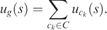
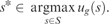
Constraints may be ascribed different levels of importance by simply weighting the rewards for satisfying them, or by using a positive monotonic transform of constraint reward (Schiex et al., Reference Schiex, Fargier and Verfaillie1995). The objective is then to find a global configuration of variable states, s*, such that
It is also possible to include hard constraints in this formalization of DCOPs. This is achieved by augmenting the additive global utility function with a multiplicative element that captures the hard constraints:

where HC and SC are the set of hard and soft constraints, respectively, and where the payoff for satisfying each hard constraint is 1, and 0 if the hard constraint is violated. The consequence is that if any of the hard constraints are violated the global utility is 0, while if all of the hard constraints are satisfied the global utility increases with the number of soft constraints satisfied. One downside to including hard constraints in this manner is that the strict monotonicity of ug(s) is lost, meaning that a change in a variable's state may satisfy additional constraints, but not increase the global utility. If this is the case, it implies that the global utility possesses many local, sub-optimal stable points that are only quasi-local maxima.
2.2 Distributed constraint optimization problems
A DCOP is produced when a set of autonomous agents each independently control the state of a subset of the variables of a constraint optimization problem, but share the goal of maximizing the rewards for satisfying constraints (i.e. they aim to jointly maximize ug(s)). For pedagogical value, and without loss of generality, we consider the case where each agent controls only one variable. We notate the set of agents involved in a constraint by Nc, and the set of constraints in which i is involved is Ci. Each agent has a private utility function, ui(s), which is dependent on both its own state and the state of all agents that are linked to any constraint c ∈ Ci. We call these agents i's neighbours, notated v(i), and notate those neighbours involved in a specific constraint ck as  . The simplest and, arguably, most natural, choice of utility function in DCOP is to set each agent i's utility to the sum of the payoffs for constraints that it is involved in:
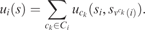
Now, each agent's choice of strategy is guided by its desire to maximize its private utility, but this utility is strategically dependent on the strategies of its neighbours. In order to analyze such a system, we use the tools and terminology of non-cooperative game theory.
2.3 Non-cooperative games
A non-cooperative game, Γ = 〈N, {Si, ui}i ∈N〉, is comprised of a set of agents N = 1, …, n, and for each agent i ∈ N, a set of strategies Si, with  , and a utility function
 . Note that, in the context of DCOPs, we can use si to represent the ‘state of a variable’ and ‘strategy of an agent’ interchangeably. A joint-strategy profile s ∈ S is referred to as an outcome of the game, where S is the set of all possible outcomes, and each agent's utility function specifies the payoff they receive for an outcome by the condition that, if and only if the agent prefers outcome s to outcome s′, then ui(s) > ui(s′). That is, each agent's utility function ranks their preferences over outcomes. We will often use the notation s = {si, s −i}, where s −i is the complimentary set of si.
In non-cooperative games, it is assumed that an agent's goal is to maximize its own payoff, conditional on the choices of its opponents. A best-response correspondence, βi(s −i), is the set of agent i's optimal strategies, given the strategy profile of its opponents,  . Stable points in such a system are characterized by the set of Nash equilibria.
Definition 1 A joint-strategy profile, s*, such that no individual agent has an incentive to change to a different strategy, is a Nash equilibrium:

In a Nash equilibrium, each agent plays a best response:  for all i ∈ N. As such, in a game where agents independently choose which strategy to adopt, a Nash equilibrium is a stable point where no individual agent has an incentive to change their strategy.
We can also define a strict Nash equilibrium, which is a necessary component of many proofs of convergence in game theory, by replacing the inequality in Equation (3) with a strict inequality. The implication of this substitution is that in a strict Nash equilibrium, no agent is indifferent between their equilibrium strategy and another strategy, which is not the case in a Nash equilibrium. This also leads us to a definition of non-degenerate games. In general, a non-degenerate game is one for which in every mixed-strategy Nash equilibrium, all agents mix over the same number of pure strategies. When considering pure-strategy Nash equilibria, non-degeneracy means that for any pure-strategy equilibrium profile of its opponents, an agent's best-response correspondence contains only one strategy. Consequently, all pure-strategy Nash equilibria in non-degenerate games are strict. Note that this condition does not exclude the possibility of a game possessing multiple Nash equilibria. Rather, it ensures that at most one equilibrium exists for each of an agent's pure strategies.
2.4 Hypergraphical games
In DCOPs, an agent's utility is a function of the constraints in which it is involved, and is only dependent on its own and its neighbours’ states: that is, ui(si, sv (i )). Therefore, we can model a DCOP game using a compact representation known as a hypergraphical game. In more detail, hypergraphical games are a model used to represent non-cooperative games that have strict independences between players’ utility functions (Papadimitriou & Roughgarden, Reference Papadimitriou and Roughgarden2008). In this model, the independences in the agents’ utility functions are used to decompose an n-player global game into local games, each involving fewer players. This decomposition can be thought of as a bipartite graph, in which one set of nodes corresponds to the set of players and the other represents the games played between them. Then, any agent i whose strategy affects others players’ payoffs in a particular local game is connected to that local game node. This representation is more compact than the standard normal form whenever the global game can be factored into sufficiently many local games, and when the maximum number of neighbours an agent has, k, can be bounded k ⪡ n, it is exponentially smaller than the standard form (Papadimitriou & Roughgarden, Reference Papadimitriou and Roughgarden2008).
Formally, a hypergraphical game comprises a set of local games: Γ = {γ 1, γ 2, …, γm}. Each local game is a tuple  , where N γ ⊆ N is the set of agents playing γ and
 is the payoff to i from its involvement in γ. For each player, Si is identical for each game, and player i chooses one strategy to play in all of the local games it is involved in (i.e. i plays the same strategy in each local game). As in DCOPs, agent i's neighbours, v(i), are the agents with whom agent i shares a local game node, with those neighbours involved in a specific local game γ notated v γ(i). Agents are usually involved in more than one local game, with the set of local games in which i is involved denoted Γi. Agent i's total payoff for each strategy is given by the sum of payoffs from each local game it is involved in:

In the context of DCOPs, each constraint is modelled by a local game, and agents are linked to the local games corresponding to their constraints. Each agent's utility then is given by the sum of the utilities from constraints that it is involved in (as in Equation 2).
More generally, the hypergraphical game model generalizes the model of factor graphs (Kschischang et al., Reference Kschischang, Frey and Loeliger2001). Factor graphs can be used to represent DCOPs, as well as graphical probability models such as Bayesian networks and Markov random fields. In both the factor graph and hypergraphical game models, each variable node comes under the control of an agent, and, typically, the global utility to be optimized is the sum or product of each agent's utilityFootnote 6. The difference between the models lies in what the hyperedges represent. In factor graphs, a hyperedge (factor node) represents a single valued function, which is its contribution to the utility of the agents it contains. In contrast, each hyperedge in a hypergraphical game represents an arbitrary non-cooperative game, in which agents’ payoffs may differ. In other words, a factor graph is a special case of a hypergraphical game in which each local game gives an identical payoff to all the agents involvedFootnote 7: that is, local games in a DCOP are team games, which are a subclass of potential games.
2.5 Potential games
The class of potential games is characterized as those games that admit a function specifying the participant's joint preference over outcomes (Monderer & Shapley, Reference Monderer and Shapley1996b). This function is known as a potential function and, generally, it is a real-valued function on the joint-strategy space (the Cartesian product of all agents’ strategy spaces), defined such that the change in a unilaterally deviating players utility is matched by the change in the potential function. A potential function has a natural interpretation as representing opportunities for improvement to a player defecting from any given strategy profile. As the potential function incorporates the strategic possibilities of all players simultaneously, the local optima of the potential function are Nash equilibria of the game; that is, the potential function is maximized by self-interested agents in a system. Importantly, we will show that the global utility function acts as a potential for a DCOP game. We now formalize some of the key concepts related to potential games.
Definition 2 (Potential Games). A function  is a potential for a game if

A game is called a potential game if it admits a potential.
Intuitively, a potential is a function of action profiles such that the difference induced by a unilateral deviation equals the change in the deviator's payoff.
The usefulness of potential games lies in the fact that the existence of a potential function for a game implies a strict joint preference ordering over game outcomes. This, in turn, ensures that the game possesses a number of particularly desirable properties, which we will use to analyze the behaviour of various algorithms in the coming sections.
Theorem 3 (Monderer & Shapley, Reference Monderer and Shapley1996b). Every finite potential game possesses at least one pure-strategy equilibrium.
Proof. Let P be a potential for a game Γ. Then the equilibrium set of Γ corresponds to the set of local maxima of P. That is, s is an equilibrium point for Γ if and only if for every i ∈ N,

Consequently, if P admits a maximal value in S (which is true by definition for a finite S), then P possesses a pure-strategy Nash equilibrium. □
Now, pure-strategy Nash equilibria are particularly desirable in decentralized agent-based systems, as they imply a stable, unique outcome. Additionally, strict Nash equilibria must be pure by definition. Mixed-strategy equilibria, on the other hand, imply a stationary, probabilistically variable equilibrium strategy profile. Also note that it is likely that more than one Nash equilibrium exists, and that some of those Nash equilibria will be sub-optimal.
Building on this, a step in a game Γ is a change in one player's strategy. An improvement step in Γ is a change in one player's strategy such that its utility is improved. A path in Γ is a sequence of steps, φ = (s 0, s 1, …, s t …), in which exactly one player changes their strategy at each step t. A path has an initial point, s 0, and if it is of finite length T, a terminal point s T. A path φ is an improvement path in Γ if for all t, ui(s t−1) < ui(s t) for the deviating player i at step t. A game Γ is said to have the finite improvement property if every improvement path is finite.
Theorem 4 (Monderer & Shapley, Reference Monderer and Shapley1996b). Every improvement path in an ordinal potential game is finite.
Proof. For every improvement path φ = (s 0, s 1, s 2, …) we have, by Equation (2):

Then, as S is a finite set, the sequence φ must be finite. □
The finite improvement property ensures that the behaviour of agents who play ‘better responses’ in each period of the repeated game converges to a Nash equilibrium in finite time. Taken together, these properties ensure that a number of simple adaptive processes converge to a pure-strategy Nash equilibrium in the game (as discussed further for specific algorithms in Section 4).
Using the definitions above, we can construct a mapping between potential and hypergraphical games. To begin with, we note that Young (Reference Young1998) shows that if every pairwise utility dependency corresponds to a bimatrix potential game between two agents, then the entire game is a potential game. Building on this, we generalize Young's result to hypergraphical potential games comprising several n-player games, a result upon which the rest of the paper hinges.
Theorem 5 A hypergraphical game Γ is a potential game if every local game γ is a potential game.
Proof. Sufficiency is shown by constructing a potential function for the hypergraphical game Γ. Each local game γ has a potential P γ(s), so a potential for the entire game, P, can be constructed by aggregating the potentials of the local games:

Now, given a strategy profile s, a change in a deviating player i's payoff is captured by changes in the values of potential functions, P γ(s), of the local games i is involved in, Γi, so the following statements hold:
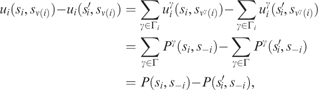
where the second line flows from the first because the potential function between independent agents is a constant value, and the third line flows from the second by definition. □
Therefore, if every local game has a potential, the global hypergraphical game also has a potential. In Section 2.6 we will use a specific instance of Theorem 5 to show that DCOP games are potential games. This result uses the fact that team games are a subclass of potential games. Formally, a team game is a game in which all agents share a common payoff function, and this common payoff function is a potential for the game: that is,  ∀ i ∈ N.
2.6 Distributed constraint optimization problems as graphical potential games
In Equation (2), we defined agents’ utilities such that all agents involved in a constraint receive the same reward from that constraint; in other words, each constraint game is a team game. Consequently, we can make the following remark, which is a corollary of Theorem 5.
Corollary 6 Every DCOP game in which the agents’ private utilities are the sum of their constraint utilities is a potential game.
As per Theorem 5, a potential for such a DCOP game can be constructed by aggregating the local (team) games’ potential functions. Of course, this is exactly the global utility function ug, specified in Equation (1). Now, for completeness, observe that, because a change in i's strategy only affects the neighbours of i, v(i), the following statements hold:
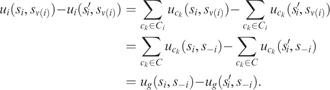
Thus, any change in state that increases an agent's private utility also increases the global utility of the systemFootnote 8.
Now, when the scenario requires employing a local approximate best-response algorithm, the solution to a DCOP game is produced by the independent actions of the agents in the system. These solutions are located at stable points in the game; that is, for this class of algorithms, the Nash equilibria of the DCOP game characterize the set of solutions to the constraint optimization problem. We have shown that DCOP games are potential games, so we are assured that at least one pure-strategy Nash equilibrium exists. Furthermore, the globally optimal strategy profile corresponds to a pure-strategy Nash equilibrium, because it is a maximum of the potential. We emphasize that in most DCOPs many Nash equilibria exist, and furthermore, many of those will be sub-optimal. This is particularly the case when hard constraints are incorporated, because, as noted earlier, the global utility function is likely to have many local quasi-maxima wherever a hard constraint is violated.
Recently, however, quality guarantees on worst-case Nash equilibria and k-optima for DCOP games have been derived for certain classes of DCOP games (Pearce & Tambe, Reference Pearce and Tambe2007; Bowring et al., Reference Bowring, Pearce, Portway, Jain and Tambe2008). In more detail, k-optima are a generalization of Nash equilibria, applicable only to DCOPs, that are stable in the face of deviations of all teams of size k and less. The payoff to a team, x is defined as

where Cx = ∪i ∈xCi; that is, the team utility is the sum of all constraint utilities any member of x is involved in, counting each constraint only once. Nash equilibria are k-optima with k = 1, and every (k + 1)-optimum is also a k-optimum, so every k-optima is a Nash equilibriumFootnote 9. The key result is that the worst-case k-optimal solution improves as the value of k increases (i.e. as the maximum size of the deviating coalitions considered increases). Given this, the worst-case k-optimum results can be used to guarantee lower bounds on the solutions produced by some DCOP algorithms. However, bounds only exist for k greater than or equal to the constraint arity of the problem, so bounds do not exist for Nash equilibria in problems involving anything other than unary constraints.
We now present an example DCOP—a graph colouring game. We give this example because it is often used as a canonical example in this domain, and it shows that complicated payoff structures may be constructed by combining simple constraint games.
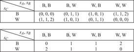
Example 1 In graph colouring, neighbouring nodes share constraints, which are satisfied if the nodes are in differing states. Consider the following graph colouring problem, where each node can be either black or white, that is, Si = {B, W}, and the associated 2 × 2 constraint game:
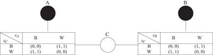
Now, in this example, agents A and B each effectively play the game above with agent C, while agent C plays the composite game below, constructed by combining the constraint games it is playing with each neighbour. In the tables below, A and B are column players and C is the row player. The top table contains the payoffs (uA, uB, uC), and a potential for the game is given in the lower table:
In the above we have described the utility functions that define a DCOP game, the associated solution concepts, and some important properties of DCOP games that flow from their classification as potential games. However, what is not specified in the above formulation are the processes by which agents adjust their states in order to arrive at a solution. These are the algorithms used to solve the game, and are the topic of the next section. Before continuing, however, we make one general comment regarding both the interpretation of the repeated game and the strategy adaptation process. We interpret the agents as being involved in several rounds of negotiation about the joint state of their variables before playing the DCOP game once. Alternatively, we could justify this perspective by assuming that the agents suffer from extreme myopia, so that they do not look beyond the immediate rewards for taking an action, as is standard in much of the literature on learning in repeated games. Either way, the only Nash equilibria that are supported are the Nash equilibria of the one-shot DCOP game; that is, the Folk Theorem for repeated games does not come into consideration.
3 A framework for local approximate best-response distributed constraint optimization problems algorithms
In this section we describe the basic components of the main DCOP algorithms present in the literature, including those developed for solving potential games, those developed for DCOPs generally, and those designed to solve specific problems that may be represented by a DCOP. By doing this, we open a way to investigate synergies that arise by combining seemingly disparate approaches to solving DCOPs using local approximate best-response techniques. This is pursued further in the next section, where we analyze how differences in the algorithms affect their behaviour and the solutions they produce, and propose novel algorithms incorporating the best features of each. However, first of all, an explication of the basic framework we use to analyze all the algorithms and the design space is provided.
As noted above, in all the DCOP algorithms we discuss, agents act myopically, in that they only consider the immediate effects of their actions (or state changes, see the discussion above). Given an appropriate trigger, the individual agents follow the same basic two-stage routine, comprising state evaluation, which produces some measure of the desirability of each state, followed by a decision on which action to take, based on the preceding state evaluations. The system-wide process that triggers an agent's processes is given by an adjustment schedule, that controls which agent adjusts its state at each point in time. In more detail:
State evaluation: Each algorithm has a target function that it uses to evaluate its prospective states. The target functions are typically functions of payoffs, and sometimes take parameters that are set exogenously to the system or updated online. Additionally, some algorithms may make use of information about the past actions of agents to compute the value of the target function.
Decision rule: The decision rule refers to the procedure by which an agent uses its evaluation of states to decide upon an action to take. Typically an algorithm prescribes that an agent selects either the state that maximizes or minimizes the target function (depending on the target function in question), or selects a state probabilistically, in proportion to the value of the target function for that state.
Adjustment schedule: In many algorithms (particularly those addressed in the game theory literature), the scheduling mechanism is often left unspecified, or is implicitly random. However, some algorithms are identified by their use of specific adjustment schedules that allow for preferential adjustment or parallel execution. Furthermore, in some cases the adjustment schedule is embedded in the decision stage of the algorithm.
Note that communication does not figure explicitly in this framework. Information is communicated between agents for two purposes: (i) to calculate the value of their target function, or (ii) to run the adjustment schedule. Given this, the communication requirements of each algorithm depend on the needs of these two stages. For example, algorithms that use random adjustment protocols only transfer information between agents to calculate the value of their target function (usually just their neighbours’ states), whereas in algorithms that use preferential adjustment schedules (such as the maximum-gain messaging algorithm), additional information may be required to run the adjustment schedule.
Given this background, this section examines the forms that each of the three algorithm stages can take. In doing so, we make clear, for the first time, the many connections between the various algorithms. During this section we will be referring to many algorithms from the literature on DCOP algorithms and learning in games, the most important being:
• Best response and smooth best response (Fudenberg & Levine, Reference Fudenberg and Levine1998);
• Better-reply dynamics (Mezzetti & Friedman, Reference Mezzetti and Friedman2001);
• DSA (Tel, Reference Tel2000; Fitzpatrick & Meertens, Reference Fitzpatrick and Meertens2003);
• Maximum-gain messaging algorithm (Yokoo & Hirayama, Reference Yokoo and Hirayama1996; Maheswaran et al., Reference Maheswaran, Pearce and Tambe2005);
• Adaptive play (Young, Reference Young1993) and spatial adaptive play (Young, Reference Young1998);
• Distributed simulated annealing (Arshad & Silaghi, Reference Arshad and Silaghi2003);
• Fictitious play (Brown, Reference Brown1951; Robinson, Reference Robinson1951) and smooth fictitious play (Fudenberg & Kreps, Reference Fudenberg and Kreps1993; Fudenberg & Levine, Reference Fudenberg and Levine1998);
• Joint-strategy fictitious play (JSFP; Marden et al., Reference Marden, Arslan and Shamma2009b);
• Regret matching (Hart & Mas-Colell, Reference Hart and Mas-Colell2000) and variants of regret monitoring (Arslan et al., Reference Arslan, Marden and Shamma2007);
• Stochastic coordination-2 algorithm and maximum-gain messaging-2 algorithm (Maheswaran et al., Reference Maheswaran, Pearce and Tambe2005).
We now discuss the various target functions that are used in DCOP algorithms, and then examine different decision rules and adjustment schedules used in DCOP algorithms.
3.1 State evaluations
The way in which a local iterative approximate best-response algorithm searches the solution space is, in the largest part, guided by the target function used by agents to evaluate their choice of state. The most straightforward approach is to directly use the payoffs given by the utility functions to evaluate states. Some shortcomings of this approach, such as slow convergence, poor search and sub-optimal solutions, are addressed by more sophisticated specifications of the algorithm's target function. These include using measures of expected payoff, average regret, and aggregated utilities. The next subsection addresses using immediate payoffs as a target function, while subsequent ones examine the more sophisticated target functions.
3.1.1 Immediate payoff and change in payoff
As noted above, the simplest target function that a DCOP algorithm can use to evaluate its strategy is to directly use its private utility function, ui(si, s −i), producing typical ‘hill-climbing’ or ‘greedy’ behaviour. This leads the system to a Nash equilibrium, which corresponds to a local potential-maximizing point. The best-response dynamics is the most well-known example of such an approach.
Furthermore, many algorithms, including the DSA, the distributed breakout algorithm and the maximum-gain messaging algorithms, use the amount to be gained by changing strategy as a target function. This is a simple perturbation of the utility function achieved by finding the difference between the current state's value and the value of all other possible states. For many decision rules, using either the gain or the raw utility function as an input will produce the same result. However, when it is useful to differentiate between those states that improve payoff and those that do not, or when the decision rule used can only take non-negative values as inputs, gain in payoff is the appropriate target function.
Agents using this target function to update their evaluation of states only need to observe the current state of their neighbours to run the algorithm, and do not need to communicate any further information. However, the use of such a target function can often result in slow convergence.
3.1.2 Expected payoff over historical frequencies
In order to speed up convergence, an algorithm can use the expected payoff for each state over historical frequencies of state profiles as a target function. These can be constructed in at least two different ways, either by maintaining an infinite memory of past actions, as in the fictitious play algorithms, or a finite memory, as in variants of adaptive play.
First, we consider the infinite memory case, and the fictitious play target function in particular. Let agent j's historical frequency of playing  , be defined as
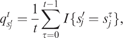
where  is an indicator function equal to one if
 is the strategy played by j at time τ, and zero otherwise. This may be stated recursively as

Now,  may be interpreted as i's belief that its opponent, j, will play strategy
 at time t. Agent i's belief over each of its opponents’ actions as a vector of historical frequencies of play for each j ≠ i is

and i's belief over all of its opponents’ actions is the set of vectors  . Following this, i's expected payoff for playing
 , given
 , is then:

where, in general, S −i = ∪j ≠i ∈NSj. However, note that in any hypergraphical game, such as a DCOP game, q −i and S −i may be replaced with qv (i ) and Sv (i ), respectively.
The classical fictitious play and smooth fictitious play algorithms use this measure of expected payoff as a target function. Variations of fictitious play that use other methods to update the agent's belief state have been suggested, many of which are contained in the broad family of generalized weakened fictitious play processes (Leslie & Collins, Reference Leslie and Collins2006). For example, in situations where an agent can only observe its payoff and has no knowledge of its neighbours’ actions, the expected payoff may be calculated as the average received payoff to each action. This is known as cautious or utility-based fictitious play (Fudenberg & Levine, Reference Fudenberg and Levine1995), and, as noted by Arslan et al. (Reference Arslan, Marden and Shamma2007), is effectively a payoff-based reinforcement learning algorithm. Additionally, Crawford (Reference Crawford1995) suggests a weighted fictitious play process for highly variable environments, in which the contribution of past observations to an agent's belief are exponentially discounted.
A similar infinite memory process, called JSFP, was introduced by Marden et al. (Reference Marden, Arslan and Shamma2009b). In this process, each agent keeps track of the frequency with which its opponents play each joint strategy s −i, rather than their individual strategy frequencies. In this case, let i's belief over its opponents’ joint-strategy profiles,  , be given by the fraction of times it observes each joint profile. Each agent's expected payoff given this belief is then:

This can be expressed more simply as
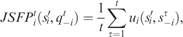
where  is the strategy profile of the agent's opponents at time τ. Furthermore, this target function can be specified recursively, which only requires agents to maintain a measure of the expected payoff for each state, rather than the full action history:

where  is the fictitious payoff to i for each element of Si given its opponents’ profile at t.
Marden et al. (Reference Marden, Arslan and Shamma2009b) show that the classical fictitious play and the JSFP target functions coincide in all two-player games. As an example of the usefulness of the hypergraphical game representation, we now show that the classical fictitious play and the JSFP target functions are identical in all binary hypergraphical games (i.e. every local game is a two-player game). To begin with, in any hypergraphical game, Equation (6) can be expressed in terms of the sum of utilities from local games:

Now, in a binary hypergraphical game, the product term is redundant because an agent has only one opponent in each local game, so using  , we can rewrite the above as

where j γ is i's opponent in γ. The expression above can be simplified because the combination of summing over all  and the indicator function can be replaced by taking the average of the payoffs actually received in each local game over time. This gives
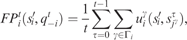
which, like the JSFP target function, admits a recursive specification:
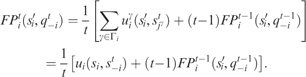
This form of classical fictitious play for binary hypergraphical games is identical to the definition of the JSFP target function stated in Equation (7).
We now consider a class of processes that evaluate the expected payoff for each state over historical frequencies of state profiles computed from samples taken from a finite memory, called adaptive play (Young, Reference Young1993). In adaptive play, agents maintain a finite history over their opponents’ actions, and construct an estimate of their mixed strategies by sampling from this history. Each individual only has a finite memory, of length m, and recalls the previous m actions taken by opponents. On each play of the game, each individual takes a sample of size k ≤ m from this memory, and computes an estimate of its opponents’ actions from this sample. That is, i's belief over j's actions, q(sj)i,t , is given by the proportion of times that j has played strategy sj in the sample of size k. Then, as in fictitious play, i's expected payoff for playing  , given
 , is given by

All of the adaptive play variants use this type of state evaluation, with various constraints on the relative values of m and k. In particular, spatial adaptive play was described in Young (Reference Young1998) as a variation of adaptive play in which both the memory m and the sample size k are 1, and in which only a single agent updates its strategy each time step.
The fictitious play, JSFP and adaptive play target functions have the same communication requirements as algorithms that use the immediate payoff for an action as a target function, because at each point in time each agent only needs to know the values of s −i in order to update its evaluation of each of its states.
3.1.3 Average regret for past actions
Another approach that can be used to speed up convergence is to measure the average ‘regret’ for not taking an action, where the regret measure for a particular strategy at a particular time is the difference between the payoff that would have been received for playing that strategy at time τ and the strategy that was actually chosen at τ. The average of these differences over the history of repeated play is the average regret for not adopting that particular strategy consistently over the entire history of play:

This target function is also known as external regret. Like the measure of expected payoff based on joint strategies discussed above, the average regret target function can be specified recursively, only requiring the agents to maintain a measure of average regret for each state:

Hart and Mas-Colell (Reference Hart and Mas-Colell2000) use this target function to construct their regret matching algorithm, and use it to characterize an entire class of adaptive strategies (Hart & Mas-Colell, Reference Hart and Mas-Colell2001a). It is also used as the target function for a distributed simulated annealing method for finding the Nash equilibria of games (La Mura & Pearson, Reference La Mura and Pearson2002). Like fictitious play, many variants of the method of updating regrets have been suggested. For example, a variation of average regret for situations where an agent can only observe its own payoff is known as internal regret (Blum & Mansour, Reference Blum and Mansour2007). This method calculates regret as the difference between the average payoff for choosing each state in the past and the received payoff for the state selected at a particular time. In this way it is analogous to cautious fictitious play.
Another example, proposed by Arslan et al. (Reference Arslan, Marden and Shamma2007), is a regret-based target function in which past regrets are weighted by a constant value. In other words, past regrets are exponentially discounted, or the agents have ‘fading memory’:

where (1−ρ) is the discount factor, 0 < ρ ≤ 1.
Again, this target function uses the same observations as algorithms that use the immediate payoff, fictitious play, JSFP and adaptive play target functions payoff for an action as a target function, because at each time step, an agent only needs to know the values of s −i in order to update its regret for each of its states.
3.1.4 Aggregated immediate payoffs
One inconvenient aspect of the above target function specifications is that they are prone to converging to sub-optimal equilibria (in the absence of some ergodic process such as a random perturbation to payoffs, as will be discussed in Section 3.2). A number of algorithms avoid this problem by using aggregated payoffs to evaluate states. However, these algorithms have significantly increased communication requirements, as agents pass information regarding the value of each state, rather than just indicating their current state.
The maximum-gain messaging-2 algorithm and stochastic coordination-2 algorithm both use a pairwise aggregate of local utility functions to evaluate the joint state of any two agents, i and j:

where the final term adjusts for the double counting of any constraints shared by the agents. This target function allows the agents to evaluate synchronized state changes, and can be used to avoid the worst Nash equilibria in the system by converging only to 2-optima. As mentioned in Section 2.2, Pearce and Tambe (Reference Pearce and Tambe2007) show that the worst-case 2-optimum solution to a DCOP game is greater than that for a Nash equilibrium, or 1-optimum. Thus, this result implies that an algorithm that uses a pairwise aggregated target function has a higher lower bound solution than any algorithm that only converges to a Nash equilibrium.
Furthermore, Maheswaran et al. (Reference Maheswaran, Pearce and Tambe2005) propose two families of k-coordinated algorithms—the maximum-gain messaging-k and stochastic coordination-k algorithms—that use locally aggregated utilities for coalitions of k agents, which each converge to an element of their respective set of k-optima. However, although the number of messages communicated at each step to calculate the aggregated utilities increase linearly with the number of neighbours each agent has, the size of each message increases exponentially with the size of the coalitions. These factors make constructing algorithms that aggregate the utilities of large coalitions of agents infeasible.
3.2 Decision rules
A decision rule is the procedure that an agent uses to map the output of its target function to its choice of strategy. The decision rule used by most DCOP algorithms is either the argmax or argmin functions, or probabilistic choice functions. The choice between these two serves an important purpose, as it determines whether the algorithm follows a hill-climbing trajectory or is stochastic. In the former case, the algorithm produced may converge quickly—or may even be anytime—but it may not be able to escape from the basin of attraction of a local maximum.
On the other hand, adding ergodicity allows the algorithm to escape from the basin of attraction of a sub-optimal Nash equilibrium (or local maximum of the potential function), but at the cost of sometimes degrading the solution quality. Proportionally probabilistic decision rules map payoffs through a probabilistic choice function to a mixed strategy (Fudenberg & Levine, Reference Fudenberg and Levine1998). As such, states with a higher-valued target function are chosen with greater probability, but states with lower payoffs than the current state are sometimes chosen. This allows the agents in the system to escape local optima. However, it also means that the algorithm is no longer an anytime optimization algorithm. Two such probabilistic choice functions are the linear and multinomial logit choice models. The simulated annealing decision rules add ergodicity by probabilistically moving to a lower utility state in proportion to its distance from the current state's utility, while always moving to states with higher utility. Finally, the ε-greedy decision rule, commonly used in machine learning, selects a state with the highest valuation with probability (1−ε) and chooses uniformly from the remaining states with probability ε. We now consider these rules in more detail.
3.2.1 Argmax and argmin decision rules
The argmax function (or, equivalently, the argmin function) returns the state with the highest (lowest) valued target function. Two variations of this decision rule are present in the literature, which differ in how they handle multiple situations where multiple states correspond to the highest value of the target function. These two variants of the argmax function are discussed in the context of the DSA in Zhang et al. (Reference Zhang, Wang, Xing and Wittenburg2005), where the algorithms are named DSA-A and DSA-B, respectively. In the first, which we call argmax-A, if the agent's state at t−1 is one of the states that maximizes the target function, then it is the state selected at t. Otherwise, a new state is randomly chosen with equal probability from the set of target function maximizing states. That is, the agent only changes its state if it improves the value of its target function. In the second variant, argmax-B, an agent randomly selects a new state from the set of target function maximizing states, without regard for the state at t−1. Note that in non-degenerate games, every best response is unique, so the two variants of the argmax function behave identically.
A benefit is that using the argmax function in conjunction with an immediate reward target function and a suitable adjustment schedule (such as in the maximum-gain messaging algorithm) is that the resulting algorithm can be ‘anytime’, in that each new solution produced is an improvement on the last. However, one potential drawback of this technique is its dependence on initial conditions, even when the algorithm is not anytime. It is possible that the initial random configuration of states places the system outside the basin of attraction of an optimal Nash equilibrium, meaning that an algorithm using the argmax decision rule can never reach an optimal point. To avoid this scenario, a probabilistic decision rule may be used instead.
3.2.2 Linear probabilistic decision rules
The linear probabilistic decision rule produces a mixed strategy with probabilities in direct proportion to the target value of each state:
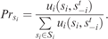
This model is only appropriate when the target function supplies a non-negative input. Although this appears to be quite a substantial limitation, the linear probabilistic choice rule is useful in certain circumstances. For example, the regret matching algorithm uses the linear probabilistic choice function with negative regrets set equal to zero, so that they are chosen with zero probability (Hart & Mas-Colell, Reference Hart and Mas-Colell2000). Another example is the better-reply dynamic, in which an agent randomly chooses a new state from those which (weakly) improve its payoff (Mezzetti & Friedman, Reference Mezzetti and Friedman2001).
3.2.3 Multinomial logit decision rules
One probabilistic decision rule that can accept negative input is the multinomial logit decision rule (Anderson et al., Reference Anderson, de Palma and Thisse1992), known in statistical mechanics as the Boltzmann distribution:
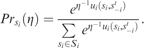
Here states are chosen in proportion to their reward, but their relative probability is controlled by η, a temperature parameter. If η = 0 then the argmax function results, while η = ∞ produces a uniform distribution across strategies, which results in the state of the system following a random walk. Depending on the specifics of the problem at hand, the temperature can be kept constant or may be decreased over time. If an appropriate cooling schedule is followed, the later case is referred to as a ‘greedy in the limit with infinite exploration’ decision rule in the online reinforcement learning literature (Singh et al., Reference Singh, Jaakkola, Littman and Szepesvari2000). The multinomial logit choice function is used in typical specifications of smooth best response, spatial adaptive play (Young, Reference Young1998), and smooth fictitious play (Fudenberg & Levine, Reference Fudenberg and Levine1998; Hofbauer & Sandholm, Reference Hofbauer and Sandholm2002).
3.2.4 Simulated annealing decision rules
The simulated annealing decision rule is a probabilistic decision rule that works by randomly selecting a new candidate state, k, and accepting or rejecting it based on a comparison to the current state (Metropolis et al., Reference Metropolis, Rosenbluth, Rosenbluth, Teller and Teller1953; Kirkpatrick et al., Reference Kirkpatrick, Gelatt and Vecchi1983). All improvements in the target function are accepted, while states that lower the value of the target function are only accepted in proportion to their distance from the current state's value. For example, the case where the target function is given by the agent's private utility function gives the following decision rule:

where ui(k, s −i) and ui(si, s −i) are the candidate and the current state's payoffs, respectively. As with the multinomial logit choice model (Equation 12), η is a temperature parameter. If η = 0 then only states that improve the target function are accepted, while η = ∞ means that all candidate states are accepted, and consequently, as with the multinomial logit function, the state of the system follows a random walk. The temperature may be kept constant, resulting in an analogue of the Metropolis algorithm (Metropolis et al., Reference Metropolis, Rosenbluth, Rosenbluth, Teller and Teller1953), or may be decreased over time as in a standard simulated annealing optimization algorithm (Kirkpatrick et al., Reference Kirkpatrick, Gelatt and Vecchi1983). Distributed simulated annealing has been proposed as a global optimization technique for DCOPs (Arshad & Silaghi, Reference Arshad and Silaghi2003), and a simulated annealing algorithm based on average regret has been suggested as a computational technique for solving the Nash equilibria of general games (La Mura & Pearson, Reference La Mura and Pearson2002).
3.2.5 The ε-greedy decision rule
One particularly common decision rule used in online reinforcement learning is known as ε-greedy. Under this rule, an agent selects a state with maximal expected reward with probability (1−ε), and a random other action with probability ε, that is,

Like the multinomial logit decision rule, the exploration parameter, ε, can be kept constant or may be decreased over time. Under specific conditions on the rate of decrease, the later case is another example of a ‘greedy in the limit with infinite exploration’ decision rule (Singh et al., Reference Singh, Jaakkola, Littman and Szepesvari2000). This decision rule is used in many variations of adaptive play (e.g. Young, Reference Young1993).
3.3 Adjustment schedules
An adjustment schedule is the mechanism that controls which agents adjust their state at each point in time. The simplest schedule is the ‘flood’ schedule, where all agents adjust their strategies at the same time. Beyond this, adjustment schedules can be divided into two groups: random or deterministic. The former are typically run by each agent independently, and can produce sequential or parallel actions by agents. The latter often require agents to communicate information between themselves in order to coordinate which agent adjusts its strategy at a given point in time, with priority usually given to agents that can achieve greater gains or are involved in more conflicts. Other times the ordering is decided upon in a preprocessing stage of the algorithm.
3.3.1 Flood schedule
Under the flood schedule, all agents adjust their strategies at the same time. This schedule is in essence the Jacobi iteration method (Press et al., Reference Press, Flannery, Teukolsky and Vetterling1992). It is frequently used in applications of local greedy algorithms (e.g. Matthews & Durrant-Whyte, Reference Matthews and Durrant-Whyte2006), and in implementations of fictitious play (e.g. Leslie & Collins, Reference Leslie and Collins2006) and some variants of adaptive play (e.g. Young, Reference Young1993).
A problem commonly observed with algorithms using the flood schedule, particularly greedy algorithms, is the presence of ‘thrashing’ or cycling behaviour (Zhang et al., Reference Zhang, Wang, Xing and Wittenburg2005). Thrashing occurs when, as all agents adjust their states at the same time, they inadvertently move their joint state to a globally inferior outcome. Furthermore, it is possible that a set of agents can become stuck in a cycle of adjustments that prevents them from converging to a stable, Nash equilibrium outcome. In theory, the potential for these types of behaviours to occur means that convergence cannot be guaranteed, while in practice they are detrimental to the performance of any algorithm using the flood schedule.
3.3.2 Parallel random schedules and inertia
Parallel random adjustment schedules are simply variations of the flood schedule, in which each agent has some probability p of actually changing its state at any time step. In the computer science literature on DCOPs, p is known as the ‘degree of parallel executions’ (Zhang et al., Reference Zhang, Wang, Xing and Wittenburg2005), whereas in the game theory literature it is commonly referred to as choice ‘inertia’ (e.g. Mezzetti & Friedman, Reference Mezzetti and Friedman2001; Marden et al., Reference Marden, Arslan and Shamma2009b).
Now, this type of adjustment schedule does not ensure that thrashing is entirely eliminated. However by selecting an appropriate value of p, thrashing and cycling behaviour can be minimized, producing an efficient algorithm with parallel execution without increasing the communicational requirements. Furthermore, inertia is essential to the convergence proofs of various processes, such as the better-reply dynamics and JSPF. This is the adjustment schedule used by the DSA, regret matching, and JSFP with inertia.
3.3.3 Sequential random schedules
The group of adjustment schedules that we call sequential random schedules involve randomly giving one agent at a time the opportunity to adjust its strategy, with agents selected by some probabilistic process. The motivation for using this adjustment schedule is grounded in the convergence proofs for many of the adaptive procedures taken from the game theory literature. In particular, the finite improvement property of potential games directly implies that agents that play a sequence of ‘better responses’ converge to a Nash equilibrium in a finite number of steps. This property is used to prove the convergence of spatial adaptive play and a version of Fictitious Play with sequential updating (Berger, Reference Berger2007).
Now, sequential procedures do not allow for the parallel execution of algorithms in independent subgraphs, where thrashing is not a concern, or for the execution of algorithms whose convergence can be guaranteed without asynchronous moves. However, they do ensure that agents do not cycle or thrash, which is a risk with using the flood or parallel random adjustment schedules.
In practice, there are a number of ways to implement this type of schedule. A particularly straightforward approach, which ensures that all agents have an opportunity to adjust their state is given by dividing time into segments, with each agent randomly selecting a point from a uniform distribution over the segment at which to adjust its strategy. Agents then adjust their states sequentially and in a random order, which satisfies the assumptions of the theoretical convergence results. However, such a schedule may depend on an external or synchronized clock. This type of schedule is essentially a form of Gauss–Seidel iteration, in which the order of updating is shuffled each cycle (Press et al., Reference Press, Flannery, Teukolsky and Vetterling1992). We refer to this schedule as a shuffled sequential schedule. Another simple approach would be to give each agent a mechanism that triggers action according to a probabilistic function of time, such as an exponential distribution, which can be run on an internal clock. In this process the probability of any two agents adjusting their state at the same time is zero. This could be called a sequential random exponential schedule. A final suggestion is to use token-passing to maintain sequential updates.
3.3.4 Maximum-gain priority adjustment schedule
The maximum-gain messaging algorithm takes its name from the type of adjustment schedule it uses (Yokoo & Hirayama, Reference Yokoo and Hirayama1996; Maheswaran et al., Reference Maheswaran, Pearce and Tambe2005). This preferential adjustment protocol involves agents exchanging messages regarding the maximum gain they can achieve. If an agent can achieve the greatest gain out of all its neighbours, then it implements that change, otherwise it maintains its current state. The maximum-gain messaging adjustment schedule avoids thrashing or cycling, as no two neighbouring agents will ever move at the same time.
3.3.5 Constraint priority adjustment schedule
A second preferential adjustment schedule, the constraint priority adjustment schedule, works by allocating each agent a priority measure based on the number of violated constraints it is involved with. This is the type of adjustment schedule used by the APO algorithm.
4 Local approximate best-response algorithm parametrization
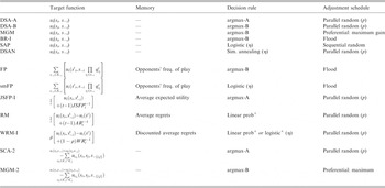
In this section we discuss how the different components of a DCOP algorithm, as identified in Section 3, affect the quality and timeliness of the solutions it produces. As an overview, Table 1 presents the parameterization of the main local approximate best-response DCOP algorithms highlighted in Section 3: two versions of the DSA (DSA-A and DSA-B), the maximum-gain messaging algorithm (MGM), the better-reply dynamic with inertia (BR-I), spatial adaptive play (SAP), distributed simulated annealing (DSAN), fictitious play (FP) and smooth fictitious play (smFP), JSFP with inertia (JSFP-I), adaptive play (AP), regret matching (RM), weighted regret monitoring with inertia (WRM-I), the stochastic coordination-2 algorithm (SCA-2), and the maximum-gain messaging-2 algorithm (MGM-2). In this table, the relationships between the algorithms are clearly shown, in terms of the components used to construct each of them.
Parameterization of the main local approximate best-response DCOP algorithms

DCOP = distributed constraint optimization problem; DSA = distributed stochastic algorithm; MGM = maximum-gain messaging; BR-I = better-reply dynamic with inertia; SAP = spatial adaptive play; DSAN = distributed simulated annealing; FP = fictitious play; smFP = smooth fictitious play; JSFP-I = joint-strategy fictitious play with inertia; RM = regret matching; WRM-I = weighted regret monitoring with inertia; SCA-2 = stochastic coordination-2 algorithm.
Before beginning the detailed discussion, we define some of the terms we use in the analysis. In particular, we say an algorithm converges in finite time if there exists a value T after which the joint state of the agents is guaranteed to be a Nash equilibrium. An algorithm almost surely converges if the probability of the agents’ joint state being a Nash equilibrium converges to 1 as the number of time steps tends to infinity. An algorithm converges in distribution if the distribution over joint states converges to some specified distribution as time tends to infinity. Typically, the specified distribution is the Boltzmann distribution over the joint state with temperature η that maximizes the global utility. Note that almost-sure convergence and convergence in distribution do not prevent the algorithm from moving arbitrarily far from a specified outcome, but only that these moves occur with decreasing probability (Grimmett & Stirzaker, Reference Grimmett and Stirzaker2001). An algorithm is called anytime if at each time step the solution it produces is at least as good as the one produced at the previous time step. Finally, a joint strategy is called absorbing if it is always played after the first time it is played, as is standard in the stochastic processes literature (e.g. Grimmett & Stirzaker, Reference Grimmett and Stirzaker2001).
We now move on to discuss in detail how the algorithms are related and where they differ, and furthermore, how this affects their behaviour and the solutions they produce. In the process, we will sketch several convergence proof techniques, and will extend some existing convergence proofs to cover algorithms with similar structures. First, we analyze those algorithms that use immediate reward or change in payoff as a target function. This allows us to demonstrate clearly how different decision rules and adjustment schedules affect the convergence properties of the algorithms. We then discuss algorithms that use recursive averaging measures, such as expected reward or regret, as target functions.
4.1 Immediate reward and gain-based algorithms
In this section we discuss those algorithms that use immediate payoff, change in payoff, or aggregated measures of either to evaluate states. In so doing, we will demonstrate three techniques of proving the convergence of a DCOP algorithm, which exploit the existence of a potential function in three different ways. Importantly, these techniques can be extended to similar algorithms that comprise common components. As such, we discuss the algorithms in groups based on their convergence proofs, beginning with MGM, which has the anytime property and converges to Nash equilibrium. Second, we consider DSA and BR-I, which rely on almost-sure convergence to Nash equilibrium. Third, we discuss SAP and DSAN, which, by virtue of the particular probabilistic decision rules they employ, can be shown to converge in distribution to the global maximum of the potential function. Finally, we discuss the convergence of the MGM-k and SCA-k to k-optima, and relate their convergence to that of MGM and DSA, respectively.
4.1.1 Anytime convergence of MGM
We begin with MGM. In ordinal potential games, MGM converges to a Nash equilibrium and is an anytime algorithm (Maheswaran et al., Reference Maheswaran, Pearce and Tambe2005). This is because agents act in isolation (i.e. none of their neighbours change strategy at the same time), so their actions only ever improve their utility, which implies an improvement in global utility (by Equation 5). Furthermore, by the same reasoning, the finite improvement property ensures that this algorithm converges to a Nash equilibrium in finite timeFootnote 10.
4.1.2 Almost-sure convergence of DSA and BR-I
Although similar in construction to MGM, neither DSA nor BR-I are anytime, as it is possible that agents who change state at the same time find themselves in a worse global state than they began in. However, using almost-sure convergence, we can show the following: DSA-A (DSA using argmax-A) almost surely converges to a Nash equilibrium, and DSA-B and BR-I almost surely converge to a strict Nash equilibrium. Although similar results have been published (e.g. Young, Reference Young1998; Mezzetti & Friedman, Reference Mezzetti and Friedman2001), for pedagogical value, we present a proof of the convergence of DSA-B to a strict Nash equilibrium, which we use as a template for sketching other convergence proofs. We will refer back to the steps presented in this proof when discussing the convergence of other algorithms in future sections.
Proposition 7 If a strict Nash equilibrium exists, then DSA-B almost surely converges to a strict Nash equilibrium in repeated potential games.
Proof. A strict Nash equilibrium is an absorbing strategy profile under DSA-B's dynamics; that is, once in a strict Nash equilibrium, no agent will change their strategy. Now, for any non-Nash equilibrium outcome, there exists a minimal improvement path, terminating at a Nash equilibrium. Denote the length of the longest minimal improvement path from any outcome to a Nash equilibrium L Γ. The rest of this proof involves showing that as t→∞, the probability that the complete longest minimal improvement path has been traversed goes to 1.
In a game consisting of N agents using DSA-B to adapt their state, for any probability of updating p ∈ (0, 1), the probability that only one agent changes state at a particular time step is given by p(1−p)N−1. Consider the probability that at some time step, the agent selected to change its state is able to improve its utility (i.e. is part of an improvement path). This probability is at least p(1−p)N−1/N, which is its value when at that time step, the improvement step is unique. Thus, at any time, t, the probability of traversing the longest minimal improvement path of length L Γ, is at least:
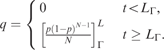
Note that whenever t ≥ L Γ, q is greater than zero, because p ∈ (0, 1) and N and L Γ are finite. Following this, in a sequence of t steps, the probability of traversing the longest minimal improvement path and converging to a Nash equilibrium at time t, pconv(t), simply follows a geometric distribution, with positive probabilities beginning at time step L Γ:

Consequently, we can express the cumulative probability of converging by t, Pconv(t)—the sum of pconv(t)—as
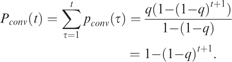
Then, as t→∞, (1−q)t + 1→0, so the probability that a complete longest minimal improvement path is traversed goes to 1 as the number of rounds tends towards infinity. □
The convergence proof for DSA-A follows the same argument, except that all Nash equilibria are absorbing. For BR-I, the proof is identical. This is because the only difference between DSA-B and BR-I is that the former selects the best response while the latter selects a better response, and these cases are treated in the same way with respect to the finite improvement property: That is, the finite improvement property ensures that all improvement paths are finite, whether they be best-response or better-response paths.
We have now described two methods of proving the convergence of a DCOP algorithm. The first shows that an algorithm is anytime, and that it improves until it reaches a Nash equilibrium. The second technique begins by characterizing the absorbing states of an algorithm. Then, by the finite improvement property, at any time in the future there is some non-negative probability of the algorithm entering the absorbing state. Therefore, the algorithm almost surely converges.
The algorithms discussed so far have produced individual best or better responses. However, one common drawback of these approaches is that if these algorithms converge to sub-optimal equilibria, they cannot escape. One technique used to get around this problem is to use stochasticity in the decision rule. A second is to aggregate agents’ utilities and allow coordinated, joint changes in state. These two techniques are discussed in the following two sections.
4.1.3 Convergence of SAP and DSAN to the global optimum
Both SAP and DSAN use a stochastic decision rule to escape from local maxima. Specifically, by using the logistic or simulated annealing decision rules, they can move between basins of attraction of local maxima.
In potential games, SAP is known to converge to a distribution that maximizes the function:

which is given by the Boltzmann distribution with temperature parameter η (Young, Reference Young1998, Chapter 6). By setting η low, this algorithm approximates the optimal joint state, and at any point in time has a high probability of having the optimal configuration.
Furthermore, regarding both SAP and DSAN, when the temperature parameter of these decision rules are decreased over time according to an appropriate annealing schedule (i.e. η∝1/log t), they are known to converge to the Nash equilibrium that maximizes the potential function (Kirkpatrick et al., Reference Kirkpatrick, Gelatt and Vecchi1983; Young, Reference Young1998; Benaim et al., Reference Benaïm, Hofbauer and Sorin2005, Reference Benaïm, Hofbauer and Sorin2006). That is, they converge to the global optimum.
4.1.4 Convergence of MGM-k and SCA-k to k-optima
A second technique used to escape local maxima is to use a target function that aggregates local utilities to evaluate joint-strategy changes by teams of agents. This is the approach used by MGM-2 and SCA-2, which both check for all joint changes in state by pairs of agents (as in Equation 11), and the families of MGM-k and SCA-k algorithms generally.
Similar to MGM, under MGM-2, only isolated pairs of agents act at a given step, so any change only improves the global utility, and the algorithm only terminates when it reaches a 2-optimum, rather than a Nash equilibrium (Maheswaran et al., Reference Maheswaran, Pearce and Tambe2005). The almost-sure convergence of SCA-2 is proven using the same method as DSA, except that the absorbing states are the set of 2-optima. However, note that bounds on worst-case 2-optima only exist for DCOPs containing unary and binary constraints, so the benefits of using MGM-2 in DCOPs with constraint arity greater than 2 are unclear. Nonetheless, these proofs can easily be extended to convergence to k-optima for the corresponding algorithms.
4.2 Algorithms using averaging target functions
In this section, we discuss averaging algorithms that use variations of the expected payoff over historical frequencies of actions and average regret target functions. We begin with the fictitious play family of algorithms, before considering regret-based algorithms.
4.2.1 Fictitious play algorithms
The term ‘fictitious play’ is often used to denote a family of adaptive processes that use the expected payoff over historical frequencies of actions as a target function (Fudenberg & Levine, Reference Fudenberg and Levine1998). Now, all versions of fictitious play that use historical frequencies as a target function and the argmax decision rule (regardless of the adjustment schedule used) have the property that if play converges to a pure-strategy profile, it must be a Nash equilibrium, because if it were not, some agent would eventually change their strategy.
The standard fictitious play algorithm, described in Table 1 as FP, uses the expected payoff over historical frequencies as a target function (Equation 6) and the argmax-B decision rule, and agents follow the flood schedule and adjust their state simultaneously. A proof of the convergence of FP to Nash equilibrium in weighted and exact potential games is given by Monderer and Shapley (Reference Monderer and Shapley1996a). Specifically, in repeated potential games, this algorithm converges in beliefs; that is, each agents’ estimate of its opponents’ strategies, which are used to calculate each of its own strategies’ expected payoffs, converge as time progresses. This process induces some stability in an agent's choice of strategy because an agent's current strategy is based on its opponents’ average past strategies, which means that an agent's belief moves through its belief space with decreasing step size. Consequently thrashing and cycling behaviour is reduced, compared to, say, DSA or the best-response dynamics.
The same target function and adjustment schedule are used in smFP as in FP, but, typically, the multinomial logit decision rule substitutes for the argmax rule. However, unlike SAP or DSAN, this substitution does not imply that the algorithm converges to the global maximum of the potential function. Rather, smFP converges to a Nash equilibrium, in much the same way as FP (Hofbauer & Sandholm, Reference Hofbauer and Sandholm2002). Nonetheless, in practice, using the logit decision rule does, on average, produce better quality solutions than the argmax rule. Leslie and Collins (Reference Leslie and Collins2006) show how to analyze smFP when the temperature parameter reduces over time and smFP approximates FP in the limit.
The dynamics of all versions of JSFP are quite different to that of FP. Specifically, strict Nash equilibria are absorbing for any algorithm that uses the JSFP target function (Equation 7) and argmax-A as a decision rule. This is because if agents have beliefs that induce them to play a strict Nash equilibrium, these beliefs are reinforced each time the strict Nash equilibrium is played.
To date, convergence to Nash equilibrium has not been shown for a version of JSFP that operates on the flood schedule. However, regarding the version that operates on the parallel random schedule, JSFP with inertia (JSFP-I), its proof of convergence to strict Nash equilibria is based on a similar argument to that for the convergence of DSA (Marden et al., Reference Marden, Arslan and Shamma2009b). Given that strict Nash equilibria are absorbing, all that needs to be shown is that at any given time step, JSFP-I has some positive probability of visiting a strict Nash equilibrium. Now, under JSFP-I any unilateral change in strategy climbs the potential. Then, as with DSA, when inertia is added to the agents’ choice of action (i.e. by using the parallel random adjustment schedule), the probability that a sequence of unilateral moves numbering at least the length of the longest improvement path occurs is strictly positive. Therefore, over time, the probability of entering the absorbing state approaches one. As with FP, because agents’ current strategies are based on average past joint strategies, the JSFP-I process produces relative stability in an agent's choice of strategy, and as a consequence thrashing and cycling behaviour is reduced. Additionally, because JSFP-I uses the parallel random schedule, the number of messages required each time step to run the algorithm is less than FP.
4.2.2 Adaptive play algorithms
The AP variants we consider here are all of those in which an agent takes a sample of size k from a finite memory of the previous m plays of the game to evaluate their expected rewards for state (Equation 8) and chooses a state using the ε-greedy choice rule, and all of the agents operate using the flood schedule (note that this excludes SAP). A subset of these algorithms can be shown to converge to a strict Nash equilibrium, using results from perturbed Markov processes (Young, Reference Young1993, Reference Young1998). The key elements of the proof are as follows.
First, call the particular joint memory maintained by the agents at t, the memory configuration. Note that if ε = 0, then the memory configurations containing only strict Nash equilibria are absorbing for any k ≤ m. That is, with no random play, if all agents’ memories contain only a single strict Nash equilibrium, that equilibrium will be played from there on. Second, using a resistance tree argument (Young, Reference Young1993), it can be shown that from any memory configuration, for any 1/|v(i)|ε > 0 (where v(i) are i's neighbours), the probability of moving along an improvement path towards a strict Nash equilibrium is greater than that for a movement away. As such, over time the probability of traversing an entire (finite) improvement path goes to 1. This result holds provided that the sample size k ≤ m/(L Γ + 2), where L Γ is the longest minimal improvement path from any joint-action profile to a strict Nash equilibrium. Building on this, as ε→0, the probability of the memory configuration consisting entirely of one strict Nash equilibrium also goes to 1. Then, in the limit, this strict Nash equilibrium is absorbing.
4.2.3 Regret matching and weighted regret monitoring algorithms
Like the variations of fictitious play, algorithms that use the average regret for past actions to evaluate states also come in many different forms. Here we limit our attention to the regret matching (RM) and weighted regret monitoring with inertia (WRM-I) algorithms, which show contrasting behaviour as a result of a small difference in the target function they employ.
RM uses the average regret for past actions (Equation 9) in conjunction with a linear probabilistic decision rule (which assigns zero probability to strategies with negative regret values) to decide on a strategy, with agents adjusting by the parallel random schedule. RM converges to the set of correlated equilibria (a generalization of Nash equilibria) in all finite games (Hart & Mas-Colell, Reference Hart and Mas-Colell2000), however, it does not necessarily converge to Nash equilibria. Nonetheless, it is easy to see that by using this target function, an agent's worst performing strategies are ruled out earliest, and although the use of a linear probabilistic decision rule does cause some thrashing, the presence of negative regrets lessens these effects.
On the other hand, WRM-I does converge to a pure-strategy Nash equilibrium in potential games (Arslan et al., Reference Arslan, Marden and Shamma2007). This algorithm uses a target function that discounts past regrets by a constant weight (Equation 10) and the parallel random schedule, and may be specified with any probabilistic decision rule that only selects a strategy from those with non-negative average regret (e.g. linear+ or logit+). In the case of the linear+ decision rule, WRM-I differs from RM only in the target function used. The proof of its convergence is similar to DSA and JSFP, and proceeds as follows. First, note that the target function used in WRM-I discounts past regrets (Equation 10). As a consequence, if a given strict Nash equilibrium is played consecutively a sufficient number of times, it will be the only strategy for which any agent has a positive regret. Additionally, the converse also holds: if each agent has only one strategy with non-negative regret, the corresponding joint strategy must be a Nash equilibrium. Second, the decision rules used in WRM-I only select from those strategies with non-negative regret. Therefore, if the joint regret-state is ever at a point where only one joint strategy has a positive regret for every agent, the algorithm will continue to select that joint strategy. Let us call this region in the agents’ joint regret-space an equilibrium's joint regret sink. Third, the final step in the proof is to show that there is some strictly positive probability that the agents’ joint regret enters an equilibrium's joint regret sink. This is achieved via the finite improvement property and the use of inertia, in an argument similar to that used in the proof of convergence of DSA. Note that if past regrets are not discounted, then convergence to a Nash equilibrium cannot be guaranteed, and the algorithm may not even converge to a stationary point (as is the case in RM).
5 Conclusions
In this paper, we focused on local approximate best-response algorithms for DCOPs, for optimization in domains where communication is difficult, costly or impossible, and in which optimality can be traded off against timeliness or computational and communicational burden. Specifically, our key contribution is a framework for analyzing local approximate best-response algorithms for DCOPs—that is, algorithms that operate by having agents exchange messages that contain only their strategy. Our framework captures many algorithms developed in both the computer science and game theory literatures. Moreover, we argue that the appropriate solution concept for the class of local approximate best-response algorithms is the Nash equilibrium condition. Given this, our framework is built on the insight that when formulated as non-cooperative games, DCOPs form a subset of the class of potential games. In turn, this allowed us to apply game-theoretic methods to analyze the convergence properties of local approximate best-response algorithms developed in the computer science literature.
In general, our framework is based on a three-stage decomposition that is common to all local approximate best-response DCOP algorithms. Given an appropriate trigger, an individual agent enters a state evaluation stage, which produces some measure of the desirability of each state. This is followed by a decision on which action to take, based on the preceding state evaluations. Then, the system-wide process that controls which agent adjusts its state at each point is given by an adjustment schedule. We populate our framework with algorithm components, corresponding to the three stages above, that are used in existing algorithms, and which can be used to construct novel algorithms.
Our framework can assist system designers by making the pros and cons of the various DCOP algorithm configurations clear. To illustrate this, we constructed three novel hybrid algorithms from the components identified in our parameterization. We evaluated these hybrids alongside eight existing algorithms taken from both the computer science and game theory literatures. Our experimental results show that an algorithm's behaviour is accurately predicted by identifying its constituent components. For example, algorithms that use fictitious play-like target functions and an argmax decision rule converge to a Nash equilibrium, but by varying the adjustment schedule, a designer may trade off between convergence time and communication use. Thus, a system designer may use our framework to tailor a DCOP algorithm to suit their mix of requirements, whether they be high quality solutions (bute.g. in the presence of bandwidth restrictions), rapid convergence (such as in real-time settings), or low communication costs (e.g. in the presence of resource constraints such as battery life). Furthermore, we expect most of our experimental results to generalize to other problems that fall within the class of hypergraphical potential games.
Generally in field of DCOPs, the main problems requiring attention involve extending the basic, static model with known payoffs and lossless communication to encompass the real-world aspects of typical DCOP application domains. In more detail, the most salient of these aspects can be broken into the following groupings:
Online learning of unknown rewards: online learning of reward functions poses a difficult problem in DCOPs, particularly if coordinated search of the joint-action space is not possible. It is important to consider the differences in approaches to the problem that are needed if the goal is to maximize the long-term reward (as is often addressed in Markov decision processes) or to find a ‘good enough’ solution quickly (as in optimal stopping problems). This problem can be further extended by considering the case were rewards are not just unknown, but observations of them are noisy, or even stochastic.
Dynamic problems: DCOPs have proven to be very useful for describing static problems, but their usefulness for dynamic and stochastic problems is not clear. There is, however, scope for exporting techniques for DCOPs to decentralized Markov decision processes and partially-observable Markov decision processes in order to identify tractable classes of those problems and to, subsequently, develop algorithms based on DCOP solution techniques. Furthermore, if decentralized optimization mechanisms that produce timely solutions are desirable in many static scenarios, then there is an even greater demand for principled decentralized approximation heuristics for real-time sequential decision-making in dynamic scenarios, and we believe the approaches developed here represent a first step in developing such techniques.
Communication: the model of communication adopted in this paper is a natural, although naive one. Communication in real-world applications of DCOPs is lossy, noisy, delayed and otherwise asynchronous, and has not been systematically addressed. Similarly, we assume communication takes place over a network defined by the constraint graph. How relaxing this assumption, to consider cases where agents do not have a direct communication link with all of the agents their utility depends on, affects the efficacy of existing approaches is unknown.
Appendix A
The following pseudocode describes several of the algorithms discussed in this paper. The pseudocode states the computations carried out by an individual agent, and unless otherwise stated, the algorithms (including their various adjustment schedules) are implemented by each agent running the stated procedure at every time step. In all that follows, we drop the sub-script i because the pseudocode refers to an agent's internal processes. We denote an agent's strategy s ∈ S and its target function's value for strategy k as stateValue(k) or stateRegret(k), as appropriate. An agent's neighbours are indexed j ∈ v, with their joint-strategy profile notated sv. Finally, an agent's immediate payoff for a strategy k, given its neighbours’ joint-strategy profile is written u(k, sv). The algorithms listed here are the maximum-gain messaging algorithm (MGM), the DSA using the argmax-B decision rule (DSA-B), better-response with inertia (BR-I), spatial adaptive play (SAP), fictitious play (FP), smooth fictitious play (smFP), joint-strategy fictitious play with inertia (JSFP-I), and weighted regret monitoring with inertia (WRM-I).
Maximum-Gain Messaging (MGM)

Distributed Stochastic Algorithm (DSA-B)

Better-Response with Inertia (BR-I)

In SAP the agents adjust their state in a random sequence. In practice, there are a number of ways to implement this type of schedule, however, the simplest is to randomly select an agent to run the stated procedure. Note this usually means some agents may be given more than one opportunity to adjust their state in a particular time step, while other agents may have none.
Spatial Adaptive Play (SAP)

In FP and smFP, |v| is the number of neighbours an agent has, qj is a vector of the frequencies with which neighbour j has played each strategy kj in the past,  is an indicator vector with an element equal to one for the state kj played by j at time t and zero everywhere else, and
 is the size of the agent's neighours’ joint-strategy space.
Fictitious Play (FP)

Smooth Fictitious Play (smFP)

Joint-Strategy Fictitious Play with Inertia (JSFP-I)

Weighted Regret Matching with Inertia (WRM-I)