

INTRODUCTION
Exawatt (EW, 1018 W) laser will provide the new experimental methods and physical conditions to research inertial confinement fusion (Labaune et al., Reference Labaune, Hulin, Galvanauskas and Mourou2008; Nuckolls et al., Reference Nuckolls, Wood and Thiessen1972; Imasaki & Li Reference Imasaki and Li2007a; Reference Imasaki and Li2007b; Reference Imasaki and Li2008; Reference Imasaki and Li2009), weapons physics, astrophysics, solid-state physics, and so on. In 2007, Japanese researchers, K. Imasaki and D. Li, proposed that nuclear fusion can be induced by an EW laser. In the same year, the extreme light infrastructure European project provided the optical power density of a light field beyond 1025 W/cm2 by focusing ten 375 J/15 fs ultra-short laser pulses on to a small spot (Chambaret et al., Reference Chambaret, Canova, Lopez-Martens, Chériaux and Mourou2007). The High Power laser Energy Research (HiPER) project achieved fast ignition by means of a multi-beam, shot pulse laser with 100 kJ delivered in 15 ps (Dunne, Reference Dunne2006; Garrec et al., Reference Garrec, Atzeni, Batani, Gizzi, Ribeyre, Schurtz, Schiavi, Ertel, Collier, Edwards, Perlado, Honrubia and Rus2011). The focal spot size of the short pulse petawatt (PW) system for fast ignition (Moses, Reference Moses2009; Zuegel et al., Reference Zuegel, Borneis and Barty2006) is a few microns to several tens of microns (Bromage et al., Reference Bromage, Bahk, Irwin, Kwiatkowski, Pruyne, Millecchia, Moore and Zuegel2008; Baker et al., Reference Baker, Homoelle, Utternback, Stappaerts, Siders and Barty2009; Antici et al., Reference Antici, Fuchs, d'Humières, Robiche, Brambrink, Atzeni, Schiavi, Sentoku, Audebert and Pépin2009; Burkhart et al., Reference Burkhart, Bliss, Nicola, Kalantar, Lowe-Webb, McCarville, Nelson, Salmon, Schindler, Villanueva and Wilhelmsen2011; Oades et al., Reference Oades, Evans, Slark, Foster, Eagleton and Clark2004; Schwarz et al., Reference Schwarz, Rambo, Geissel, Edens, Smith, Brambrink, Kimmel and Atherton2007; Yanovsky et al., Reference Yanovsky, Chvykov, Kalinchenko, Rousseau, Planchon, Matsuoka, Maksimchuk, Nees, Cheriaux, Mourou and Krushelnick2008; Bahk et al., Reference Bahk, Rousseau, Planchon, Chvykov, Kalintchenko, Maksimchuk, Mourou and Yanovsky2004). The smaller the focal spot, the higher the required positioning accuracy of spatial coupling between laser and target. Accurate direct detection and location for small-scale focal spot is the key technical difficulties. The measurement accuracy of the small-scale focal spot position is related to the size of charge coupled device (CCD) pixel. When the focal spot is completely covered by more than one pixel, the image subdivision technology can be used to improve the measurement accuracy. When the focal spot size is equal to or smaller than the size of the CCD pixel (4–14 µm), first the focal spot size will be amplified by using defocus technique or focal spot microscope imaging method, then in image processing, which has some limitations. We put forward a high-precision hard subdivision method that can measure the information (centroid position, relative intensity distribution) of the focal spot directly and thus improve the measurement accuracy. The focal profile can be diagnosed through the obtained relative intensity distribution of the focal spot. This method avoids the introduction of aberration and chromatic aberration, which affected the location test results like the image-relaying method and also avoids the short-comings such as the instability through energy, and the small field of view which is introduced by the structural stability of the through-hole method. According to the positioning technical problem of beam-target coupling of the short (ultra-short) pulse laser, we explore the method for precise positioning of the small focal spot of the short (ultra-short) pulse, which provide technical support for short (ultra-short) pulse target systems. The results obtained in this paper can also be applied to the long pulse transmission-mode targeting system.
HIGH-PRECISION MEASUREMENT MODEL AND METHOD
Considering the threshold exposure and the saturate exposure where A/D is N bits, the single CCD pixel response model can be described by the response function f as:
 $$Z=f\lpar I\rpar =f\lpar E \cdot t \rpar =\left\{\matrix{0 {I \in \left[{0\comma \; I_1 } \right]} \cr m {I \in \left({I_m\comma \; I_{m+1} } \right]\comma \; } {m=1\comma \; \cdot \cdot \cdot\comma \; 2^N - 1} \cr {2^N - 1} {I \in \left({I_{2^N }\comma \; \infty } \right)}} \right.\comma$$
where Z is the gray value of the pixel, E is the illumination of the CCD pixel, t is the integration time of the CCD pixel received, exposure I is equal to E × t, and I 1 is the threshold exposure and I 2N −1 is the saturate exposure.
The size of a single CCD pixel is 10 µm × 10 µm and the space between pixels is 2 µm. The measurement range of the gray value is from 0 to 4095 for 12 bits CCD. Take I 1 = 100e−18 J, I m+1 − I m = 10 J, then I 2N −1 = 100e−18 + 40950 J.
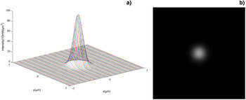
If an ideal Gaussian beam with a radius of 1 µm and the center at the origin is established, then the size is less than a single CCD pixel. The radius of the Gaussian beam spot is defined as the distance between the spot center and the position with 1/e2 of the peak energy. Intensity distribution of the spot can be described as:
 $$I=100 \times e^{ - \lpar x^2+y^2 \rpar \times 2}.$$
The intensity distribution and gray image for ideal Gaussian beam are shown in Figure 1.
(a) The intensity distribution of ideal Gaussian focal spot, where coordinates x and y are positions of each spot point in units of μm, coordinate z is the energy value of the point in units of 10 mW/μm2. (b) The gray image of the ideal Gaussian focal spot.

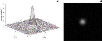
The noise from the fluctuation of the energy exposure to the CCD and from the CCD itself must be added to the ideal Gaussian spot. The intensity distribution and gray image of the ideal Gaussian beam with noise are shown in Figure 2.
(a) The intensity distribution of ideal Gaussian focal spot with noise, where coordinates x and y are positions of each spot point in units of μm, coordinate z is the energy value of the point in units of 10 mW/μm2. (b) The gray image of the ideal Gaussian focal spot with noise.

In this paper, we calculated the centroid position and the relative intensity distribution for the focal spot by obtaining the gray value for each subdivision via two-dimensional fine scanning and detailed CCD cutting (which is smaller than a pixel).
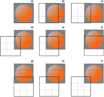
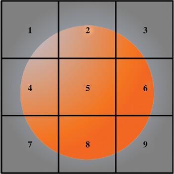
The proposed method is as follows: Adjust the position of the focal spot so that it is located within a particular pixel (assuming the size of the pixel is 10 µm). Since the focal spot is the same size as the CCD pixel, then it is divided into a number of smaller square pieces (subdivisions). Since the position of the focal spot is fixed, we snake-moved the CCD with each step distance to cut and scan the focal spot. We recorded the gray value, which is measured by the particular pixel after each step moving. The moving step is equal to the side length of the focal spot's subdivision. Dividing the focal spot into nine subdivisions, this scanning process is shown in Figure 3. The subdivisions of the original image are numbered 1 to 9 for convenience as shown in Figure 4, z is set as the corresponding gray value for each subdivision, Z is the gray value for each scan state. After scanning, the gray value for subdivision 4 can be obtained directly from the gray value in Figure 3i, where z 7 = Z i. The gray value for the subdivisions of the lower boundary and the left border in the original image can be obtained by subtracting the gray values from the two states. The gray value for subdivision 4 is the difference between the gray value for Figure 3d and Figure 3i, where z 4 = Z d − Z i. The gray value for subdivisions that are not on the lower boundary and the left border can be obtained with addition or subtraction of the gray values for the four known states. In order to get the gray value for subdivision 6, for example, the sum of the gray values for that subdivision and all of the left subdivisions in its row are obtained, the sum of the gray value is Zf − Zg. Similarly, we obtained the sum of gray values for subdivision 5 and all the left subdivisions in its row, the sum gray value is Ze − Zh, while the gray value for subdivision 6 is the difference between the two above gray-scale, namely z6 = (Zf − Zk) − (Ze − Zh). Therefore, the gray values for subdivisions 1 to 9 can be obtained.
CCD scanning process.

The small parts of subdivision.

NUMERICAL SIMULATION RESULTS
The focal spot image with a single CCD pixel size and initial overlap was divided into 101 × 101 small square pieces (subdivision). The side length of the subdivision was equal to the moving step of CCD with 0.1 µm. Set the original location of the 10 µm × 10 µm graphic which contains the focal spot in the range of x = −5–5 µm and y = −5–5 µm in numerical simulation, the initial position of a specific CCD pixel coincides with the above original location. In this paper, we simulated numerically the process of using the method of two-dimensional fine-scanning with CCD cutting a small focal spot to measure the gray distribution of the ideal Gaussian focal spot, the Gaussian focal spot with noises, respectively.
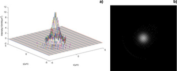
The measurement simulation results for the gray distribution of the ideal Gaussian focal spot with the diameter being less than the size of a CCD pixel is shown in Figure 5.
(a) The intensity distribution of ideal Gaussian focal spot after scanning, where coordinates x and y are positions in units of μm, coordinate z is the gray value. (b) The gray image of the ideal Gaussian focal spot after scanning.

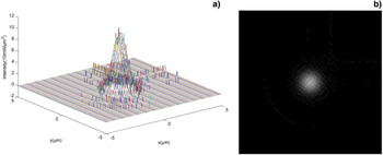
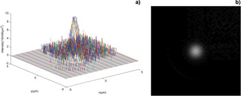
The measurement simulation results for the gray distribution of the relatively low and high noise Gaussian focal spots with the diameter being less than the size of a CCD pixel are shown in Figures 6 and 7, respectively.
(a) The intensity distribution of the relatively low noise ideal Gaussian focal spot after scanning, where coordinates x and y are positions in units of μm, coordinate z is the gray value. (b) The gray image of the ideal Gaussian focal spot with the relatively low noise after scanning.

(a)The intensity distribution of the relatively high noise ideal Gaussian focal spot after scanning, where coordinates x and y are positions in units of μm, coordinate z is the gray value. (b) The gray image of the ideal Gaussian focal spot after scanning.

The gray value for each subdivision in the gray distribution of the focal spot changed with ±1 gray value, which is caused by the data rounding up during the CCD readout process, and the other can not be ignored that optical energy enter into the detection CCD pixel when the is CCD moving. There was a serious distortion of the image after CCD scanning if the noise is too large, so the method was not suitable for high noise situations. Meanwhile, the method can not measure the focal spot that makes the CCD pixel saturated.
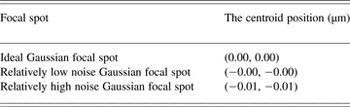
The centroid positions of the three above focal spots are calculated by the gray centroid method through the known gray values of the focal spot's points. The results were shown in Table 1.
The centroid position of the focal spot.

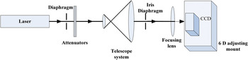
The experimental setup is shown in Figure 8. The laser source is a small-sized He-Ne laser with wavelength of 632.8 nm, which has a maximum output power of 10 mW, the beam diameter of 0.80 mm, beam divergence angle of 1.01 mrad. The CCD's main parameters are as follows: the effective resolution of 1024 × 1024, and the single pixel size of 6.45 µm × 6.45 µm. The CCD scanning control unit is a high precision six-dimensional adjusting mount, the main performance indexes are as follows: the three-dimensional translational adjustment resolution is 7 nm for piezoelectric ceramics (PZT) actuators with feedback, repetitive positioning accuracy is 15 nm RMS[sp1].
Experimental setup.

The laser focal length is 12.5 cm after attenuation, beam expander, and collimation, then focused on the photosensitive surface of the CCD, which is fixed in a high precision six-dimensional adjusting mount. The un-saturation focal spot images are collected by the CCD.
Two-dimensional snake fine scan of the focal spot using the high precision six-dimensional adjusting mount with closed-loop control of PZT, then the centroid position and intensity distribution of the focal spot are calculated. In order to verify the accuracy of the algorithm, select a specific area of 4 × 4 CCD pixels and it is equivalent to a large pixel, which size is about 25.8 µm × 25.8 µm. Set each move step as 2.58 µm, and the range of movement is 25.8 µm × 25.8 µm. The focal spot region was divided into 100 pieces. The gray value of the focal spot can be directly readout by the CCD in the initial moment when the focal spot size is larger. We reduced the gray distribution of the focal spot by two-dimensional fine scanning. The two results were compared to verify the accuracy of the algorithm. In the measurement process, on the purpose of reducing error, collected five consecutive images in each position after moving, took the average of five corresponding matrices after noise removal as the measurement data.
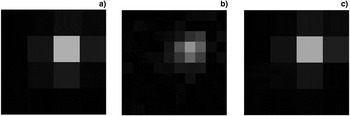
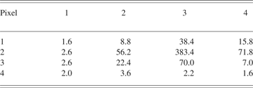
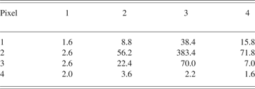
The gray image with 16 pixels of the focal spot from the data directly readout by the CCD (Fig. 9a), the centroid coordinate position of the focal spot (16.0 µm, 15.5 µm) is calculated by the gray weighted centroid algorithm. The gray value data of the focal spot directly measured by the CCD are shown in Table 2, where the gray value of each small piece read by a CCD pixel. The gray image with 100 subdivisions of the reconstruction of the focal spot obtained by the two-dimensional fine scanning with CCD is shown in Figure 9b, the centroid coordinate position of the focal spot is (16.1 µm, 14.5 µm) calculated by the gray weighted centroid algorithm. The gray image with 4 × 4 pixels as the original image of the focal spot restored by the data from scanning is also shown in Figure 9c.
(a) The gray image of the focal spot directly read out by the CCD, (b) The gray image of the focal spot by scanning, (c) The restored gray image of the focal spot.

The gray-scale data of the original spot
The main errors of the experiment are from the error made by the high precision six-dimensional adjusting mount moving and the reading error caused by the CCD readout. We calculated the errors of the x direction as an example. The coordinate x obtained by the gray centroid method has been re-written as Eq. (3).
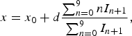 $$x=x_0+d\displaystyle{{\sum\nolimits_{n=0}^9 {nI_{n+1} } } \over {\sum\nolimits_{n=0}^9 {I_{n+1} } }}\comma$$
where x is the abscissa of the centroid of the focal spot, x 0 is the relative coordinate, d is the length of moving step, I n+1 is the sum of the gray values of the subdivisions of the No. n + 1 column of the focal spot.
x 0 is expressed as the difference between the actual coordinate (0,0) and the selected coordinate (0,0) of the bottom left corner subdivisions of the actual image. x 0 is 0 if the selected coordinate of the bottom left corner subdivision of the actual images is (0,0). The numerator and denominator of the second term in Eq. (4) can be rewritten. Let 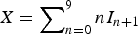 $X = \sum\nolimits_{n = 0}^9 {nI_{n + 1} }$ and
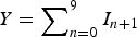 $Y = \sum\nolimits_{n = 0}^9 {I_{n + 1} } $, then we get Eqs.(4) and (5).
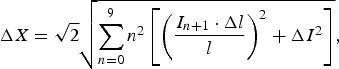 $$\Delta X=\sqrt 2 \sqrt {\sum\limits_{n=0}^9 {n^2 \left[{\left({\displaystyle{{I_{n+1} \cdot \Delta l} \over l}} \right)^2+\Delta I^2 } \right]} }\comma$$
 $$\Delta Y=\Delta I\comma$$
where I is the sum of the gray values of the focal, ΔI is the measurement error of the gray value, l is the length of the small part of subdivision, Δl is the error of each movement.
Δl is about 0.1 µm, which includes stability error and adjustment error of the high precision six-dimensional adjusting mount. The CCD read error ΔI is 5 gray values. The practical step length is 2.58 µm, the length of the subdivision is 2.58 µm. We obtained ΔX which is equal to 235.4 and ΔY is equal to 5 by bringing the data into the Eq. (5).
We only calculated the error in the second term of Eq. (3). Therefore, the error Δx of x can be obtained from Eq. (6). The calculated error of the centroid of the focal spot is 0.9 µm.
 $$\Delta x=d\displaystyle{{\sum\limits_{n=0}^9 {nI_{n+1} } } \over {\sum\limits_{n=0}^9 {I_{n+1} } }}\sqrt {\left({\displaystyle{{\Delta X} \over X}} \right)^2+\left({\displaystyle{{\Delta Y} \over Y}} \right)^2 }\comma$$
 $$\Delta x=2.58 \times \displaystyle{{3966.6} \over {690}}\sqrt {\left({\displaystyle{{235.4} \over {3966.6}}} \right)^2+\left({\displaystyle{5 \over {690}}} \right)^2 } \approx 0.89\rm \mu m.$$
CONCLUSIONS
The measurement of the spatial location of the small-scale focal spot (diameter in microns) is based on CCD hard subdivision method. We calculated the centroid position and the intensity distribution of the small-scale focal spot (diameter in microns less than the size of a CCD pixel) through the gray values of the small parts of subdivision, which are obtained by the method of two-dimensional fine scanning with CCD. The measurement accuracy of the small-scale focal spot position is about 1 µm when the fluctuations of the light energy and background noise are relatively small. The theoretical simulation is consistent with the verification experiment. As a result, we inspect the method theoretically and practically.
ACKNOWLEDGEMENTS
This work is supported by the National Natural Science Foundation of China (Grant No. 61138005 and 61008004), Program for Changjiang Scholars and Innovative Research Team in University, RFDP20102302120034, the Fundamental Research Funds for the Central Universities (Grant No. HIT. KLOF. 2010035).