


1. Introduction
In the aftermath of the global financial crisis and in the midst of the euro area debt crisis, Acharya and others (Acharya et al. Reference Acharya, Drechsler and Schnabl2012, Reference Acharya, Drechsler and Schnabl2014; Acharya and Steffen, Reference Acharya and Steffen2015) published a series of seminal papers on the relationship between banks and their sovereign in terms of risk transmission. Periods of turmoil in sovereign bond markets were judged to have the potential to destabilize banks in their jurisdiction, and across borders (Breckenfelder and Schwaab, Reference Breckenfelder and Schwaab2018; Capasso et al. Reference Capasso, D’Uva, Fiorelli and Napolitano2023). At the same time, large banks could destabilize their own sovereign. The bidirectional and mutually reinforcing nature of the sovereign-bank risk transmission is the cornerstone of this branch of literature.Footnote 1 This paper contributes by quantifying, comparing and explaining both directions of transmission. We believe this is crucial to understand contagion across sectors and for risk management both at the micro and macro levels.
In the first part, we compute Diebold and Yilmaz’s (Reference Diebold and Yilmaz2012) connectedness measures at monthly frequency, through the estimation of a VAR model with time-varying parameters and stochastic volatility à la Koop and Korobilis (Reference Koop and Korobilis2013). In details, we quantify the spillovers from the sovereign to the banking sector, as well as the reverse spillovers from the banking sector to its sovereign. Our dataset contains the 10-year sovereign bond yield spread and bank share prices of the seven largest Italian banks; we use monthly realized volatility as a measure of risk. We focus on Italy because it has a large public debt, which accounts for a large portion of banks’ assets. These are the main elements of the “diabolic loop” described by Brunnermeier et al. (Reference Brunnermeier, Garicano, Lane, Pagano, Reis, Santos, Thesmar, van Nieuwerburgh and Vayanos2011, Reference Brunnermeier, Garicano, Lane, Pagano, Reis, Santos, Thesmar, Van Nieuwerburgh and Vayanos2016), Acharya et al. (Reference Acharya, Drechsler and Schnabl2014) and, more recently for Italy, by Cafiso et al. (Reference Cafiso, Missale and Rivolta2025). Moreover, Italy has a significant number of systemically important banks with sufficiently long historical data. This allows a more detailed analysis of the relationship between sovereign risk and the banking sector, as well as a better exploration of the role of individual bank characteristics.
Contrary to common perception, and some previous conclusions on this topic (Erce, Reference Erce2020), our results show that the sovereign receives more spillover from banks than it transmits to them for most of the sample period. This means that sovereign risk is more often fed by volatility that originates in the banking sector rather than the other way around. The only exception is the period between mid-2011, which marks the beginning of the second phase of the euro area debt crisis, and the end of 2012, after several interventions by the ECB aimed at containing financial market tensions. Additionally, we conduct an event-study analysis that shows how spillovers change in response to key economic events and that policies designed to reduce them can be effective.
In the second part, we investigate some specific factors at the bank level that potentially can amplify or mitigate the observed spillovers. Building on the insight that banks’ balance-sheet structure plays a key role, we relate spillovers from the sovereign to banks, and vice versa, to banks’ balance-sheet data. Overall, our results indicate that capital adequacy acts as a key buffer, limiting both the propagation and the absorption of spillovers. Moreover, the composition of banks’ assets matters: a higher weight of securities is associated with stronger spillovers, while more traditional lending mitigates them.
In short, the contribution of our research to the existing literature is to document both the size and the direction of spillovers between the banking sector and its sovereign by applying a methodology never used in this field with bank-level data. Furthermore, we show how these spillovers evolve in response to major events and we provide evidence that policy measures designed to reduce them can be effective. Most importantly, we demonstrate that the strength of the spillovers is shaped by banks’ idiosyncratic characteristics. By focusing on spillover intensity rather than credit quantities, our findings complement existing evidence on the bank lending channel (e.g. Gennaioli et al. Reference Gennaioli, Martin and Rossi2018; Bottero et al. Reference Bottero, Lenzu and Mezzanotti2020) and provide new insights into how banks’ balance-sheet structure shapes the sovereign–bank nexus.
The rest of the paper is structured as follows. Section 2 reviews the relevant literature. Section 3 describes the methodology and the data used. Section 4 shows the results of the dynamic connectedness analysis. The regression analysis to study how much the transmission of spillovers is related to bank-specific variables is in Section 5. Section 6 concludes.
2. Literature review
Our research draws on two different strands of literature. The first examines the relationship between sovereign risk and the financial sector of the economy, while the second is methodological and relates to the approach of Diebold and Yilmaz (Reference Diebold and Yilmaz2009). The so-called sovereign-bank nexus has been modeled since Acharya et al. (Reference Acharya, Drechsler and Schnabl2012, Reference Acharya, Drechsler and Schnabl2014) and it is the object of a growing literature, which has gradually expanded to identify all transmission channels between sovereigns and banks in both directions. Using a bibliometric analysis, Bajaj et al. (Reference Bajaj, Kumar and Singh2022) show that studies on sovereign credit risk started to pick up in 2005 and, not surprisingly, gained momentum from 2012 onwards. Feyen and Zuccardi Huertas (Reference Feyen and Zuccardi Huertas2019); Kund et al. (Reference Kund, Picarelli and Solé2025) confirm the relevance of this topic by showing that the sovereign-bank nexus is growing since, globally, banks have increased their exposure to sovereigns over the past decade.
The literature has provided several possible explanations for the link between the banking sector and sovereign risk. In their seminal contribution, Acharya et al. (Reference Acharya, Drechsler and Schnabl2014) argue that during periods of financial distress, bank bailouts aimed at stabilizing the economy require substantial public spending, thereby increasing government debt and the perceived risk associated with government liabilities, which are largely held by banks.Footnote 2 Brunnermeier (Reference Brunnermeier, Garicano, Lane, Pagano, Reis, Santos, Thesmar, van Nieuwerburgh and Vayanos2011; Reference Brunnermeier, Garicano, Lane, Pagano, Reis, Santos, Thesmar, Van Nieuwerburgh and Vayanos2016) were among the first to emphasize the “diabolic loop” linking sovereign and bank solvency risks, which arises from balance-sheet effects driven by the substantial exposure of European banks to their own government bonds. Farhi and Tirole (Reference Farhi and Tirole2018) provide a theory for such a “doom loop,” formalizing how sovereign risk increases either because of the budgetary impact of lower growth or because of bailout expectations. Leonello (Reference Leonello2018) builds a model to explore the role of government guarantees in triggering the feedback loop between banking and sovereign debt crises. ECB (2016) notes that rising sovereign credit risk can also affect banks through the funding channel. As a country’s creditworthiness declines, funding conditions tighten and banks, especially those dependent on wholesale markets, face higher funding costs.Footnote 3
The central role of banks’ balance sheet in transmitting sovereign distress to the real economy has been documented empirically by Gennaioli et al. (Reference Gennaioli, Martin and Rossi2018). Using bank-level data for more than 20,000 banks across 191 countries and 20 sovereign default episodes, the authors show that banks with higher exposure to government bonds experience a significantly larger contraction in lending relative to less exposed banks during sovereign default episodes. Focusing on Italy, Bottero et al. (Reference Bottero, Lenzu and Mezzanotti2020) exploit loan-level data around the 2010 Greek bailout and show that banks with higher pre-crisis exposure to sovereign debt reduced credit supply significantly more than less exposed banks. At the macroeconomic level, Palmen (Reference Palmen2020) provides complementary evidence using a structural panel VAR for several euro area countries. The study shows that increases in sovereign default risk lead to persistent declines in bank lending and economic activity. More recently, Cafiso et al. (Reference Cafiso, Missale and Rivolta2025) focus on Italy and show that a spread shock generates valuation losses in banks’ bond portfolios, forcing banks to deleverage and reduce lending. These findings support a credit supply channel that has contractionary effects on output and, in turn, deteriorates public finances, generating a self-reinforcing vicious cycle.
Several contributions provide explanations of why the sovereign-bank nexus has expanded. Altavilla et al. (Reference Altavilla, Pagano and Simonelli2017) analyze the determinants of banks’ sovereign exposures and document that public banks’ purchases of government bonds increased significantly around major ECB liquidity injections, partly reflecting moral suasion by national governments. Related evidence is provided by Becker and Ivashina (Reference Becker and Ivashina2018), who show that during the European sovereign debt crisis governments increasingly relied on domestic banks to absorb public debt. This crowded out corporate lending, particularly in crisis countries, consistent with a form of financial repression and moral suasion. However, Rivolta (Reference Rivolta2014) showed heterogeneous consequences across countries, as she finds that ECB liquidity injections led to an increase in market spreads for lower-rated euro area countries due to flight-to-safety behavior, so that positive effects from the banking sector to sovereign debt only materialized for higher-rated countries.
Several studies document that the transmission of risk between sovereign bonds and the banking sector is also across countries (Popov and Van Horen, Reference Popov and Van Horen2015; Breckenfelder and Schwaab, Reference Breckenfelder and Schwaab2018; Capasso et al. Reference Capasso, D’Uva, Fiorelli and Napolitano2023). More closely to our framework, Fernández-Rodríguez et al. (Reference Fernández-Rodríguez, Gómez-Puig and Sosvilla-Rivero2015) suggest that slightly more than half of the total variance of forecast errors is explained by cross-country shocks rather than idiosyncratic shocks. Antonakakis and Vergos (Reference Antonakakis and Vergos2013) examine the evolution of bond yield spread spillovers in the euro area during the Great Financial Crisis and euro area debt crisis, distinguishing between core and peripheral countries. They show that spillovers within these two groups are larger than spillovers across groups, and that spillovers explain a relevant fraction of the forecast error variance. A wider international perspective is adopted by Bostanci and Yilmaz (Reference Bostanci and Yilmaz2020) who estimate the global network structure of sovereign credit risk.Footnote 4
The methodology we employ was developed by Diebold and Yilmaz (Reference Diebold and Yilmaz2009). In the last decade, it has been applied with different variations to study contagion in different fields, including the link between sovereign risk and the credit sector. The key innovation in the Diebold and Yilmaz (Reference Diebold and Yilmaz2009) approach consists in the design of a connectedness analysis based on the notion of forecast error variance decomposition obtained from a VAR model identified with the Cholesky decomposition. Diebold and Yilmaz (Reference Diebold and Yilmaz2012) improve on Diebold and Yilmaz (Reference Diebold and Yilmaz2009) by making the output independent from the order of the variables through the generalized approach of Koop et al. (Reference Koop, Pesaran and Potter1996) and Pesaran and Shin (Reference Pesaran and Shin1998). Diebold and Yılmaz (Reference Diebold and Yılmaz2014) interpret the connectedness measures of Diebold and Yilmaz (Reference Diebold and Yilmaz2012) as representing a network structure. Along this line, Le et al. (Reference Le, Dickinson and Le2022) have recently used connectedness measures to understanding the global financial network for sovereign debt. Antonakakis et al. (Reference Antonakakis, Chatziantoniou and Gabauer2020), like us, develop a dynamic connectedness analysis by means of a large time-varying parameters VAR estimated with the algorithm of Koop and Korobilis (Reference Koop and Korobilis2013).Footnote 5 Apostolakis et al. (Reference Apostolakis, Floros and Giannellis2022) is close to us both in terms of methodology and objective, as they use conditional correlation analysis and dynamic connected analysis. Their study examines the dynamics of spillovers across G7 countries and identifies which national banking sectors act as primary transmitters and receivers of financial instability. Another work applying Diebold and Yilmaz’s (Reference Diebold and Yilmaz2012) approach in a dynamic way, but to study how financial risk spreads across global stock markets is Yu et al. (Reference Yu, Ouyang, Guan and Lin2024). They investigate the channels of risk contagion combining multiple factors such as financial opening, international trade and cross-border capital flows.
3. Methodology and data
The methodology used to quantify the spillovers between the sovereign spread and banks’ share price is described in this section. Spillovers are calculated using Diebold and Yilmaz’s (Reference Diebold and Yilmaz2012) connectedness analysis (hereafter DY12), which is based on the estimation output of a Bayesian VAR with time-varying parameters and heteroskedasticity. The DY12 approach involves first estimating a VAR to obtain the forecast error variance decomposition (hereafter FEVD). This FEVD is then used to compute the connectedness measures. We underline that the DY12 method is designed and applied solely to quantify connectedness, not to control for or explain its origin. Indeed, we address such a task in a further section (5) of this work through regression analysis. In what follows, we first describe the estimation of the VAR and then briefly review the DY12 connectedness measures.
3.1. VAR estimation
The simplest approach to obtain time-varying connectedness measures is to estimate the VAR model over a rolling window (see Diebold and Yilmaz, Reference Diebold and Yilmaz2012). Rather, we use a large time-varying parameters VAR model (hereafter TVP-VAR) estimated using Bayesian methods. Indeed, it is more robust as the results do not depend on the arbitrarily-chosen size of the rolling window and no observations are lost, the TVP-VAR technique is less sensitive to the presence of outliers than other methods, and Bayesian estimation makes it possible to avoid the curse of dimensionality present in VAR models with many variables.
Our model consists of eight monthly variables, it is estimated over the period 2003–2023, and six lags are included to capture the dynamics in the data.Footnote 6 We estimate it applying the methodology of Koop and Korobilis (Reference Koop and Korobilis2013), who use the Kalman filter with forgetting factors to substantially reduce the computational burden. This approach was first applied to a VAR model by Doan et al. (Reference Doan, Litterman and Sims1984). More recently, Koop and Korobilis (Reference Koop and Korobilis2013) have developed an algorithm to estimate large TVP-VAR models and to perform model selection based on forecasting accuracy. More specifically, forgetting factors can be used to obtain analytical formulae for the posterior of the coefficients, so that no MCMC algorithm is needed. We refer to their paper and the papers cited therein for a detailed discussion of the methodology. In the following, we focus on the main features necessary to describe our setup.
A VAR model with time-varying parameters can be written in state-space form as follows:
 \begin{align} y_{t} & =X_{t}\beta _{t}+\varepsilon _{t},\nonumber \\[3pt] \beta _{t} & =\beta _{t-1}+u_{t}, \end{align}
where
 $y_{t}$
is a
 $\left (N\times 1\right )$
vector of endogenous variables,
 $X_{t}$
is a
 $ (N\times k)$
matrix containing a constant and the lags of the endogenous variables,
 $\beta _{t}$
are the coefficients that evolve over time following an AR(1) process,
 $\varepsilon _{t}$
is i.i.d.
 $N\left (0,\Sigma _{t}\right )$
and
 $u_{t}$
is i.i.d.
 $N\left (0,Q_{t}\right )$
. The matrices
 $\Sigma _{t}$
and
 $Q_{t}$
are time-varying as well and determine, respectively, heteroskedasticity in the residuals of the VAR model and the degree of time variation in the coefficients.
Classical estimation methods are based on the Kalman filter and smoother, and Gibbs sampling to draw recursively from the conditional distributions of the model’s parameters, as explained in Koop and Korobilis (Reference Koop and Korobilis2010). MCMC methods would be necessary as there is no analytical solution for the posterior distribution of the parameters. On the other hand, forgetting factors modify the Kalman filter equations replacing
 $\Sigma _{t}$
and
 $Q_{t}$
with estimates so that analytical formulae for the posterior of
 $\beta _{t}$
exist. More in details, the Kalman filter allows to compute the filtering and the prediction densities of the parameters
 $\beta$
, conditional on the observations through time
 $t$
,
 $y^{t}$
:
 \begin{align*} \beta _{t}|y^{t}\sim & N\left (\beta _{t|t},V_{t|t}\right ),\\[3pt] \beta _{t+1}|y^{t}\sim & N\left (\beta _{t+1|t},V_{t+1|t}\right ). \end{align*}
The standard formula for the variance-covariance matrix of the coefficients in the prediction step is:
 $V_{t+1|t}=V_{t|t}+Q_{t}$
. This equation can be approximated including a forgetting factor
 $\lambda$
(
 $0\lt \lambda \leq 1$
) as follows:
 \begin{equation*} V_{t+1|t}=\frac {1}{\lambda }V_{t|t}. \end{equation*}
The parameter
 $\lambda$
allows to avoid the estimation or simulation of
 $Q_{t}$
and implies that the observation
 $j$
periods in the past has weight
 $\lambda ^{j}$
in the filtered estimate of
 $\beta _{t}$
. The model also considers heteroskedastic error terms by modeling volatility with an Exponentially-Weighted Moving Average as follows:
 \begin{equation*} \hat {\Sigma }_{t}=\kappa \hat {\Sigma }_{t-1}+\left (1-\kappa \right )\hat {\varepsilon }_{t}\hat {\varepsilon }'_{t}. \end{equation*}
This equation stipulates that the covariance matrix of the measurement error is a weighted average of its lags and the residuals of the measurement equation.
In this setup, prior information is required only for the parameters
 $\beta$
. As in Koop and Korobilis (Reference Koop and Korobilis2013), we use a Normal prior that is similar to a Minnesota prior, with mean zero and variance-covariance matrix that depends on only one shrinkage parameter
 $\gamma$
. The hyperparameters of the prior are initialized using a pre-sample of three years of data, from January 2000 until December 2002.
Overall, the estimation requires the selection of the parameters
 $\lambda$
,
 $\kappa$
and
 $\gamma$
. Koop and Korobilis (Reference Koop and Korobilis2013) select optimal values for these parameters and the VAR dimensionality, with a dynamic model selection algorithm that is based on forecasting accuracy. In our application, we do not need to perform model selection across variables and since the dynamic selection procedure increases the computational burden significantly, we rely on a simpler setting: we choose the remaining parameters as in Koop and Korobilis (Reference Koop and Korobilis2012). More specifically, the forgetting factor
 $\lambda$
is set to 0.99, this value introduces a low degree of time-variation in the coefficients as it is close to the constant-coefficient case
 $\lambda =1$
. The decay factor for the volatility
 $\kappa$
is set to 0.96 following Longerstaey and Spencer (Reference Longerstaey and Spencer1996), and the parameter governing the prior shrinkage
 $\gamma$
is set to 0.99 following Raftery et al. (Reference Raftery, Karny and Ettler2010).Footnote
7
3.2. Diebold-Yilmaz connectedness analysis
Diebold and Yilmaz (Diebold and Yilmaz, Reference Diebold and Yilmaz2009, Reference Diebold and Yilmaz2012; Diebold and Yılmaz, Reference Diebold and Yılmaz2014) have proposed several connectedness measures to analyze interdependence across a set of variables. Their methodology has been widely adopted, with recent applications in the study of systemic risk and network analysis (Diebold and Yilmaz, Reference Diebold and Yilmaz2023). We first provide a simple intuition of their technique, more details follow.
Given a set of variables, the DY12 approach allows to evaluate how much a shock to one variable, comparatively, impacts itself and the others, thus creating a hierarchy of effects between the variables considered. Those effects are called spillovers and are quantified with specific connectedness measures. Diebold and Yılmaz (Reference Diebold and Yılmaz2014) interpret the size of the spillovers between two variables as the strength of the connection between two nodes of a network. Importantly, the set of variables is not chosen with the intention of explaining one of the variables with the others and vice versa, but merely to examine their relationship in terms of spillovers. The shocks are not structural as they are identified using the generalized approach of Koop et al. (Reference Koop, Pesaran and Potter1996) and Pesaran and Shin (Reference Pesaran and Shin1998). They are derived from the historical correlations but the contemporaneous relationships are not explicitly modeled. Therefore, no causal interpretation can be ascribed to the spillovers and, as in the original version of DY12 approach, there is no room to disentangle across their possible sources.
The connectedness measures are based on the generalized FEVD obtained from the estimation of a VAR model. This technique quantifies the portion of the forecast error variance of each variable that can be ascribed to shocks to the other variables over different time horizons. The starting point of the analysis is the estimation of a covariance-stationary VAR model:
 \begin{align} y_{t}={\color {magenta}{\color {black}\alpha }}+\sum _{l=1}^{P}B_{l}y_{t-l}+\varepsilon _{t}\quad \varepsilon _{t}\sim N\left (0,\Sigma \right ), \end{align}
where
 $y_{t}$
is a N-variable vector and
 $\color {magenta}{\color {black}\alpha }$
,
 $B$
and
 $\varepsilon _{t}$
are conformable vectors and matrices of coefficients, and i.i.d. shocks, respectively. This model can be inverted to obtain its moving-average representation:
 $y_{t}=\sum _{l=1}^{\infty }A_{l}\varepsilon _{t-l}$
. Here,
 $A_{l}=\sum _{i=1}^{P}B_{i}A_{l-i}$
are the coefficients from which one can derive impulse-response functions, the FEVD and the historical decomposition. In principle, these coefficients can be obtained after identifying the shocks in the system. As above-mentioned, Diebold and Yilmaz (Reference Diebold and Yilmaz2012) propose to overcome the identification problem relying on the generalized VAR framework of Koop et al. (Reference Koop, Pesaran and Potter1996) and Pesaran and Shin (Reference Pesaran and Shin1998). In this framework, the H-step ahead generalized FEVD from variable
 $j$
to variable
 $i$
is:
 \begin{align} \theta _{ij}^{g}\left (H\right )=\frac {\sigma _{jj}^{-1}\sum _{h=0}^{H-1}\left (e'_{i}A_{h}\Sigma e_{j}\right )^{2}}{\sum _{h=0}^{H-1}\left (e'_{i}A_{h}\Sigma A'_{h}e_{j}\right )}, \end{align}
where
 $\sigma _{jj}$
is the standard deviation of the error term for equation
 $j$
and
 $e_{i}$
is a selection vector with one as
 $i$
th element. Since the variance shares do not sum to one, they are normalized as follows:
 \begin{align} C_{i\leftarrow j}^{H}\equiv \widetilde {\theta }_{ij}^{g}\left (H\right )=\frac {\theta _{ij}^{g}\left (H\right )}{\sum _{j=1}^{N}\theta _{ij}^{g}\left (H\right )}. \end{align}
The measures in eq. (4) can be interpreted as percentage shares: they quantify how much each shock contributes to the forecast error variance of all variables in the model, creating a hierarchy of effects. These measures can be summarized in a connectedness table, which shows pairwise connectedness to and from each variable in the model, and total connectedness to and from others, calculated as the sum of the rows and columns (see Table 2). More in details, total connectedness to others and from others are, respectively:
 \begin{align} C_{\cdot \leftarrow j}^{H}=\sum _{i=1,i\neq j}^{N}C_{i\leftarrow j}^{H},\quad C_{i\leftarrow \cdot }^{H}=\sum _{j=1,i\neq j}^{N}C_{i\leftarrow j}^{H}. \end{align}
The index of total connectedness is the average of the off-diagonal elements of the connectedness table:
 \begin{equation} C^{H}=\frac {1}{N}\sum _{i,j=1,i\neq j}^{N}C_{i\leftarrow j}^{H}. \end{equation}
In our analysis, we focus on
 $C_{i\leftarrow j}^{H}$
and on
 $C_{j\leftarrow i}^{H}$
, the connectedness from the sovereign spread to each bank’s shares, and vice versa, to which we refer as spillStB and spillBtS respectively. We also use their directional aggregation,
 $C_{\cdot \leftarrow j}^{H}$
and
 $C_{i\leftarrow \cdot }^{H}$
, to which we refer as TspillStB and TspillBtS respectively. Spillover and connectedness are synonyms in this context. Since all variables enter the VAR in terms of volatility, we study volatility spillovers.
3.3. Data
Our analysis is based on two sets of data. The first consists of daily series: i) the share price of the banks in our sample, ii) the yield to maturity of the 10-year benchmark bond of Italy and Germany. These data come from Datastream. Daily data are aggregated to obtain monthly variables, as explained below. These variables are used for the analysis in the first step, which consists in estimating the VAR model and calculating the DY12 connectedness measures.
The second is a quarterly dataset of balance-sheet variables for the Italian banks object of our investigation. It serves for our regression analysis in the second step, in which we aim to understand how much the spillovers from the sovereign spread to the banks (spillStB), and their opposite (spillBtS), are related to bank-specific characteristics; the source is Standard & Poor’s Capital IQ.
In the following, we first motivate the sample of Italian banks used for the analysis, then describe the variables used to apply the DY12 methodology, and finally list the variables included in the regression analysis in the second step. The period under analysis is 2003–2023, for which we use data starting from 2000. The DY12 analysis in the first step is based on daily data and provides monthly measures of connectedness. These are later averaged quarterly to match the banks’ balance sheet data and to run the regression analysis at a quarterly frequency in the second step.
Sample of banks
We started with the sample of Italian listed banks for which share price series were available since 2000. Among these, we restricted the focus to banks supervised by the ECB, i.e. systemically important institutions. This resulted in eight banks, but we had to exclude Monte dei Paschi di Siena due to serious inconsistencies in its share price series over the period considered.Footnote 8 Eventually, our sample includes: (1) Banca Popolare di Sondrio, (2) Banco BPM, (3) BPER Banca, (4) Credem, (5) Intesa Sanpaolo, (6) Mediobanca, (7) Unicredit. The list of these banks, together with summary statistics of the balance sheet variables taken into account, can be found in Table 1.
Variables for DY12 analysis
We derive the DY12 connectedness measures, i.e. the spillovers, using the realized volatility of returns. As regards shares, returns are computed directly as the logarithmic difference of daily prices
 $P_{t}^{s}$
:
 \begin{equation} r_{t}^{S}=log\left (P_{t}^{S}/P_{t-1}^{S}\right ). \end{equation}
As for government bonds, to ensure consistency across asset classes, we work also with returns computed on prices derived from bond yields. First, we calculate the sovereign spread between the Italian (
 $Y_{t}^{IT}$
) and the German (
 $Y_{t}^{DE}$
) 10-year government bond yields:
 $Y_{t}^{B}=Y_{t}^{IT}-Y_{t}^{DE}$
. Second, we retrieve bond prices applying the well-known formula that links the price of a zero-coupon bond to its yield, using the spread as follows:
 \begin{equation} P_{t}^{B}=\frac {100}{\left (1+Y_{t}^{B}\right )^{n}}, \end{equation}
where
 $Y_{t}^{B}$
is in decimal units and
 $n=10$
since we consider the 10-year benchmark bond. In this way, we obtain the price of a synthetic bond that represents the price of Italian sovereign risk. Then, we use it to compute its return
 $\left (r_{t}^{B}\right )$
with eq. (7), as done for share prices.
Italian banks, summary statistics of balance-sheet ratios

Table 1. Long description
Panel A: Table summarizing balance-sheet ratios for BPER, including CAR, ROA, OEI, NPL, TAD, ISA, GLA, and MKV with mean, median, standard deviation, minimum, maximum, and observations. Panel B: Table summarizing balance-sheet ratios for BP Sondrio, including CAR, ROA, OEI, NPL, TAD, ISA, GLA, and MKV with mean, median, standard deviation, minimum, maximum, and observations. Panel C: Table summarizing balance-sheet ratios for Banco BPM, including CAR, ROA, OEI, NPL, TAD, ISA, GLA, and MKV with mean, median, standard deviation, minimum, maximum, and observations. Panel D: Table summarizing balance-sheet ratios for Credem, including CAR, ROA, OEI, NPL, TAD, ISA, GLA, and MKV with mean, median, standard deviation, minimum, maximum, and observations. Panel E: Table summarizing balance-sheet ratios for Intesa SP, including CAR, ROA, OEI, NPL, TAD, ISA, GLA, and MKV with mean, median, standard deviation, minimum, maximum, and observations. Panel F: Table summarizing balance-sheet ratios for Mediobanca, including CAR, ROA, OEI, NPL, TAD, ISA, GLA, and MKV with mean, median, standard deviation, minimum, maximum, and observations. Panel G: Table summarizing balance-sheet ratios for Unicredit, including CAR, ROA, OEI, NPL, TAD, ISA, GLA, and MKV with mean, median, standard deviation, minimum, maximum, and observations. Panel H: Table summarizing total balance-sheet ratios, including CAR, ROA, OEI, NPL, TAD, ISA, GLA, and MKV with mean, median, standard deviation, minimum, maximum, and observations.
Notes: CAR is the capital-asset ratio, ROA is return on assets, OEI is operating expenses to non-interest income, NPL is the non-performing loans ratio, TAD is total assets to deposits, ISA is investments in securities to total assets, GLA is gross loans to total assets, MKV is market value.
For both asset classes, realized volatility at monthly frequency is computed as the arithmetic average of squared returns:
 \begin{equation} RV_{m}=\frac {1}{D_{m}}\sum _{t=1}^{D_{m}}\left (r_{t}^{i}\right )^{2}, \end{equation}
where
 $r_{t}^{i}$
is the return of shares or bonds (
 $i=S,B$
) and
 $D_{m}$
is the number of days
 $t$
in month
 $m$
. In contrast to daily prices, daily returns provide dynamic information related to price changes over one day. Realized volatility (RV) is a popular statistical measure used in finance to quantify the variability of asset returns over a specific period, based on actual observed data.Footnote
9
Since VAR models are based on normality assumptions, we take the log of realized volatility to normalize its distribution.Footnote
10
The realized volatility of bank and sovereign returns is included as a dependent variable in the VAR model described in the previous subsection.
Bank’s balance-sheet variables for the regression analysis
Our regression analysis in the second part is intended to help to explain the spillover from the sovereign spread to banks, and vice versa. We use balance-sheet variables for the seven banks under investigation and, as mentioned above, the source of data is S&P Capital IQ.Footnote 11 To avoid data inconsistencies related to banks’ mergers and acquisitions, we consider only variables in terms of ratios, plus each bank’s market capitalization.
Our primary focus is on the capital-asset ratio as it is a measure of bank’s resilience to adverse shocks. Overall we use the following variables at a quarterly frequency: (1) the capital-asset ratio, CAR, in which the numerator is Tier 1 capital, as an indicator of capital adequacy; (2) return on assets, ROA, as an indicator of income performance; (3) operating expenses over non-interest income, OEI, to account for operational efficiency; (4) non-performing loans over total loans, NPL, as an indicator of asset quality; (5) total assets over deposits, TAD, as an indicator of the source of financing; (6) investments in securities over total assets, ISA, and (7) gross loans over total assets, GLA, both to account for the portfolio composition; (8) the market value, MKV, as an indicator of size and each bank’s relevance. Table 1 reports summary statistics of these variables for each bank in our sample, a more detailed discussion of their use in the context of our regression analysis is in Section 5.
4. Connectedness analysis: Spillovers between the sovereign and banks
This section presents the results of DY12 connectedness analysis. We focus on measures of connectedness, i.e. volatility spillovers, computed at the 1-month horizon. Although no relevant difference emerges with respect to the 3-month horizon, we believe that spillovers in high-frequency financial markets are particularly relevant in the short run, as their longer-term effects may blend with other events or fade away. To better understand the evolution of the spillovers, and to relate them to key economic events, we examine them also in an event study based on univariate autoregressive models.
Dynamic DY12 output

Table 2. Long description
The table presents dynamic DY12 output measures for various variables, including BPER, BP Sondrio, Banco BPM, Credem, Intesa SP, Mediobanca, and a total. The table has 10 rows and 10 columns, with column headers labeled as CAR, ROA, OEI, NPL, TAD, ISA, GLA, and MKV. Each row provides mean, median, standard deviation, minimum, maximum, and observation counts for these variables. For example, the BPER row shows mean values like 10.823 for CAR, 0.465 for ROA, and so on. The table captures the dynamic output measures and their variations across different variables, providing a detailed comparison of their performance metrics.
4.1. Dynamic connectedness
We start with an overview of the connectedness measures derived from the estimation of the TVP-VAR described in Section 3.1. The TVP-VAR yields connectedness measures at each point in time, we summarize them in Table 2 through their arithmetic average as in Antonakakis et al. (Reference Antonakakis, Chatziantoniou and Gabauer2020); values are for the 1-month horizon of the FEVD. Table 2 is organized in the usual DY12 way: it contains both directional spillover (from
 $i$
to
 $j$
) as well as total-to (from
 $i$
to
 $\sum j$
) and total-from (from
 $\sum j$
to i) by rows and columns. Values in the table are to be read as the percentage of the forecast error variance of variable
 $i$
explained by shocks to variable
 $j$
.
The first important result from the table is that the sovereign spread is a net receiver; meaning that the contagion from banks to the spread (48.32) is on average higher than from the spread to banks (39.65) and the difference is statistically significant.Footnote 12 The largest contributors are major banks, e.g. Intesa Sanpaolo and Unicredit. In general, average connectedness across entities is quite low while self-spillovers are more relevant. These results can be compared for robustness with those from the static connectedness analysis based on the same VAR, but estimated with ordinary least squares; those are in Table A1 in the appendix. The comparison confirms the main findings, i.e. the sovereign spread is a net receiver and the largest banks generate a larger spillover.
The whole point of using a TVP-VAR model for the DY12 connectedness analysis is to have a time series of the connectedness measures and therefore to explore the spillover evolution. Then, we plot the time values of the sum of the spillovers from the spread to each bank (TspillStB), and from each bank to the spread (TspillBtS), as well as their difference, in Figure 1; while the Total Spillover Index is in Figure A1 in the appendix. The Figure shows that the link between the spread and the banking sector volatility was weak until the onset of the global financial crisis. From then on, the size of the spillovers increased up to eight times, reaching values between 70 and 80 during the Euro area debt crisis. Thereafter, the measures of connectedness declined and fluctuated, alternating between decreasing and increasing trends. The last relevant increase in the measures of connectedness can be attributed to the Covid-19 pandemic. Both measures decline significantly in the last part of the sample, signaling a loosening of the link between the banking sector and the sovereign spread.
The plot shows that the sovereign spread is generally a net receiver, as for most of the period TspillBtS exceeds TspillStB. The only exception is the period between mid-2011, i.e. the beginning of the second phase of the euro area debt crisis, and the end of 2012, after several ECB interventions aimed to containing financial market tensions. Overall, this evidence is consistent with the narrative of events and with the findings of Acharya et al. (Reference Acharya, Drechsler and Schnabl2014) and Cafiso et al. (Reference Cafiso, Missale and Rivolta2025), which show that sovereign credit risk and the banking sector were closely linked and that the feedback loop between the two became large in the second half of 2008.
The connectedness measures peak on certain dates. To interpret their variation, we have included lines for major economic and policy events that are widely regarded as turning points, and are therefore particularly relevant for the transmission of spillovers in Italy.Footnote 13 We detect eight major events, which will serve for the event study in Subsection 4.3: the collapse of Lehman Brothers that represents the start of the Global Financial Crisis (September 2008); the emergence of the euro area sovereign debt crisis with the first Greek bailout and the implementation of the Securities Market Programme by the ECB (May 2010); the escalation of the crisis to core euro area countries during the Italian sovereign stress episode (July 2011); the first LTRO of the ECB (December 2011); the announcement of ECB President Mario Draghi’s “whatever it takes” commitment and of the OMT program (July 2012); the introduction of the bail-in regime amid heightened banking-sector stress in Italy (January 2016); the Italian general election resulting in political uncertainty and renewed sovereign stress (May 2018); and the onset of the Covid-19 pandemic and associated lock-down measures (March 2020).
Total directional spillovers.
Notes: Tspill-To stands for TspillStB, Tspill-From is for TspillBtS, Tspill-Net is their difference. Vertical dashed lines, from left to right: Lehman Brothers’ bankruptcy (Sept 2008), first Greek bailout (May 2010), Italian sovereign stress episode (July 2011), first ECB’s LTRO (December 2011), “whatever it takes” statement and announcement of the OMT programme (July 2012), introduction of new bail-in regulation and NPL turmoil (January 2016), Italian general election without a clear majority (May 2018), start of lockdown for COVID-19 pandemic (March 2020). 1-month FEVD used for calculations.

Directional spillovers.
Notes: Tspill-To stands for TspillStB, Tspill-From is for TspillBtS, Tspill-Net is their difference. Vertical dashed lines, from left to right: Lehman Brothers’ bankruptcy (Sept 2008), first Greek bailout (May 2010), Italian sovereign stress episode (July 2011), first ECB’s LTRO (December 2011), “whatever it takes” statement and announcement of the OMT programme (July 2012), introduction of new bail-in regulation and NPL turmoil (January 2016), Italian general election without a clear majority (May 2018), start of lockdown for COVID-19 pandemic (March 2020). 1-month FEVD used for calculations.

Figure 2. Long description
Panel A: The line graph for SpreadIT shows self-spillover values on the vertical axis ranging from 20 to 100, with time on the horizontal axis from 2008 to 2021. The graph indicates fluctuations in self-spillover over time, with notable peaks and troughs. Panel B: The line graph for Intesa displays spill-To, spill-Fm, and spill-Net values on the vertical axis ranging from 0 to 20, with time on the horizontal axis from 2008 to 2021. The graph shows trends for spill-To in blue, spill-Fm in red, and spill-Net in green, with visible interactions and variations over time. Panel C: The line graph for Unicredit presents spill-To, spill-Fm, and spill-Net values on the vertical axis ranging from 0 to 20, with time on the horizontal axis from 2008 to 2021. The graph illustrates the dynamics of spill-To in blue, spill-Fm in red, and spill-Net in green, highlighting different patterns and interactions. Panel D: The line graph for BPER shows spill-To, spill-Fm, and spill-Net values on the vertical axis ranging from 0 to 20, with time on the horizontal axis from 2008 to 2021. The graph depicts trends for spill-To in blue, spill-Fm in red, and spill-Net in green, with notable variations and interactions. Panel E: The line graph for BancoBPM displays spill-To, spill-Fm, and spill-Net values on the vertical axis ranging from 0 to 20, with time on the horizontal axis from 2008 to 2021. The graph shows trends for spill-To in blue, spill-Fm in red, and spill-Net in green, with visible fluctuations and interactions. Panel F: The line graph for BPSondrio presents spill-To, spill-Fm, and spill-Net values on the vertical axis ranging from 0 to 20, with time on the horizontal axis from 2008 to 2021. The graph illustrates trends for spill-To in blue, spill-Fm in red, and spill-Net in green, highlighting different patterns and interactions. Panel G: The line graph for Credem shows spill-To, spill-Fm, and spill-Net values on the vertical axis ranging from 0 to 20, with time on the horizontal axis from 2008 to 2021. The graph depicts trends for spill-To in blue, spill-Fm in red, and spill-Net in green, with notable variations and interactions. Panel H: The line graph for Mediobanca displays spill-To, spill-Fm, and spill-Net values on the vertical axis ranging from 0 to 20, with time on the horizontal axis from 2008 to 2021. The graph shows trends for spill-To in blue, spill-Fm in red, and spill-Net in green, with visible fluctuations and interactions.
Directional spillovers from the sovereign spread to each bank’s shares, and from each bank to the spread, at the 1-month horizon are plotted in Figure 2; the charts include the lines for the eight events mentioned above. Overall, relevant variations in the measures of connectedness are found also at the bank level around those dates. The first chart shows the self-spillover index of the Italian spread, i.e. how much of the spread’s error variance is due to its own shocks. This chart should be read in conjunction with Figure 1. It is interesting to note that this index was very high until September 2008, indicating that the contribution of the banking sector to spread volatility was negligible, and then it declined abruptly as spillovers from banks increased due to the financial and sovereign debt crises. With the easing of the sovereign debt crisis and the improvement in general economic conditions, the link to the banking sector decreased and self-connectedness increased again in 2015–2016. This link became stronger again during the Covid-19 pandemic, as self-connectedness declined. However, the subsequent recovery led to an increase in self-connectedness again. Overall, it seems clear that crisis periods are characterized by a stronger link between volatilities.Footnote 14
The results show some heterogeneity in the dynamics of the connectedness measures across banks. In general, the spillover from each bank to the spread is stronger than the opposite. This relationship is reversed for most banks during the sovereign debt crisis, however, spillStB is only slightly higher than spillBtS for Intesa Sanpaolo, Unicredit and Banco BPM also during the crisis. These are the largest Italian banks, so it is reasonable to interpret this finding as evidence of their systemic importance: their feedback on the spread is strong even in a situation of financial market turmoil. The observed heterogeneity could depend also on bank-specific characteristics and we explore this issue in Section 5.
Table 3 shows the correlation between the different directional spillovers at the bank level plotted in Figure 2. Consistent with Figure 2, the spread self-spillover is strongly and negatively correlated with spillovers from the spread to banks (spillStB), and from banks to the spread (spillBtS). On the other hand, the directional spillovers across banks (to and from) are positively correlated with each other, with coefficients indicating a high degree of co-movement. Likely, the factors discussed in Section 2 determine the strong inverse relationship between banks and the sovereign spread, some others the strong positive relationship across-banks.
Correlations across spillStB and spillBtS

Table 3. Long description
The table presents correlations between various directional spillovers at the bank level. It consists of two main sections: spillStB and spillBtS, each with correlations for Spread IT, Intesa SP, Unicredit, BPER, Banco BPM, BP Sondrio, Credem, and Mediobanca. Each section has 8 rows and 8 columns, with values indicating the correlation coefficients. For spillStB, the correlations range from 0.712 to 0.939, showing varying degrees of positive correlation. For spillBtS, the correlations range from 0.029 to 0.899, indicating both positive and negative correlations. Notable trends include strong positive correlations within the spillStB section and a mix of positive and negative correlations within the spillBtS section.
4.2. Robustness checks of the connectedness analysis
The connectedness analysis discussed in this section has undergone a series of robustness checks to confirm the reliability of our conclusions. First, we have estimated the underlying VAR with both 6 and 12 lags and found no relevant difference. Second, the coefficients from the dynamic analysis, averaged over the entire period (Table 2), have been compared with those from a static analysis based on the same VAR estimated using ordinary least squares; see Table A1 in the appendix. Overall, the magnitude of the effects is similar. Third, we have calculated the spillovers using the 1-month and 3-month horizons as basis for the FEVD. While our benchmark for the analysis is the 1-month horizon for the reasons explained, the conclusions remain the same in both cases.
4.3. Event-study analysis
Figures 1, 2 and A1 suggest that historical events may drive the evolution of the spillovers. Accordingly, to characterize the evolution of spillovers around major episodes of financial stress and policy intervention, we conduct an event-study analysis based on the total directional connectedness measures: TspillStB and TspillBtS as defined in eq. (5). A separate event-study regression is estimated for each event. For an event occurring at time
 $T$
, we define a symmetric event window spanning seven months, from three months before to three months after the event. Then, we include seven dummy variables in each regression.
Table 4 reports nine major event windows that we consider for the event study.Footnote 15 The central event month is highlighted in bold. While the central event represents the main shock of interest, the neighboring months capture closely related market, policy, or institutional developments, which we take into account in the interpretation of the results. This structure allows the event-study framework to capture both anticipation effects and short-run post-event dynamics, and accounting for the presence of other shocks occurring within the same window.
Event windows

Table 4. Long description
The table presents nine major event windows, each associated with specific dates and financial events. The events are grouped into clusters such as the Great financial crisis, Greek crisis, Early EA debt crisis, Second phase of EA debt crisis, Whatever it takes and OMT, Bail-in and banking stress, Italy political crisis, and Covid. Each row lists the cluster, date, and event. For example, the Great financial crisis cluster includes the Lehman-Brothers collapse in September 2008 and Post-Lehman panic & coordinated bailouts in October 2008. The table also includes events like the Greek deficit revelation in October 2009 and the ECB LTROs in December 2011 and February 2012. The central event month is highlighted in bold, indicating the main shock of interest, while neighboring months capture related market, policy, or institutional developments.
For each event, we estimate the following univariate regression model:
 \begin{equation} \Delta z_{t}=\alpha +\sum _{l=1}^{P}\phi _{l}\Delta z_{t-l}+\sum _{w=-3}^{3}\gamma _{w}D_{t}^{\left (w\right )}+v_{t}, \end{equation}
where
 $z_{t}$
denotes the spillover measure under consideration. The spillover measures enter the regressions in first differences, to correct their non-stationary behavior in levels. The coefficients
 $\phi _{l}$
capture the autoregressive dynamics of the series, while
 $\gamma _{w}$
measures deviations from the normal evolution of spillovers at different points in the event window. We include twelve lags of the dependent variable in each specification to account for serial correlation. Inference is based on a variance–covariance matrix that is robust to both heteroskedasticity and autocorrelation (Newey and West, Reference Newey and West1987). The event-time dummy variables
 $D_{t}^{\left (w\right )}$
are defined as:
 \begin{align*} D_{t}^{\left (w\right )}=\begin{cases} 1 & \mathrm{if}\;t=T+w\\ 0 & \mathrm{otherwise} \end{cases} \end{align*}
where
 $T$
denotes the month in which the main event occurs.
For brevity, we discuss only the results based on the 1-month horizon. The estimates for the 3-month horizon are reported in Table A2 in the Appendix and confirm the robustness of our findings to the choice of forecasting horizon.
Overall, the output reveals clear and economically meaningful patterns across the main episodes of financial stress and policy intervention (Table 5). Crisis events are generally associated with sharp increases in spillovers, while policy interventions are associated to a dampening in the volatility transmission across markets. To assess whether the response to an event differs significantly across spillover directions, Table A3 in the appendix complements the analysis with Wald tests of equality between the central-month coefficients estimated for the sovereign-to-bank and bank-to-sovereign spillover measures. A statistically-different effect emerges most of the times.Footnote 16
Event study regressions

Table 5. Long description
A table titled ’Event study regressions’ with five columns and twenty-eight rows, including the header row. The columns are labeled ’Event’, ’Date’, ’TspillStB:h1’, and ’TspillBtS:h1’. The table presents data on various financial events and policy interventions, with corresponding dates and spillover measures. Each row lists an event, its date, and the spillover values for the sovereign-to-bank and bank-to-sovereign measures. Notable events include the Lehman-Brothers collapse, Greek deficit revelation, First Greek bailout & ECB SMP, Italian sovereign debt crisis, LTRO I, Whatever it takes & OMT announcement, Bail-in in force & NPL turmoil, Italian political turmoil, and Global Covid crash & PEPP. The table shows the impact of these events on spillover measures, with significant values marked by asterisks indicating levels of statistical significance.
Notes: TspillStB is total spillover from the sovereign to banks, TspillBtS is total spillover from banks to the sovereign, h1 is for the 1-month horizon at the basis of the FEVD.
The collapse of Lehman Brothers in September 2008 marks a dramatic increase in the spillover measures. The strongest response is in spillovers from banks to the sovereign, consistent with the origin of the crisis in the banking sector and its rapid propagation to the sovereigns; this is confirmed also by the Wald test.
The revelation of the Greek fiscal deficit in October 2009 is associated with a decrease in both directional spillover measures. This pattern may reflect the fact that, at that stage, financial markets still perceived Greece’s fiscal difficulties as largely country-specific rather than as a source of broader systemic risk. However, since our analysis focuses exclusively on Italy, these results should be interpreted with caution. This also applies to the downgrade of Greek debt in December 2009, which is associated to a decline in the spillover measures too.
The early phase of the euro area debt crisis generated a significant increase in the spillovers already in February 2010, but particularly in May 2010 when the Greek bailout occurred and the ECB implemented the Securities Market Programme. The increase in spillovers appears quantitatively larger along the sovereign-to-banks direction (the Wald test confirms) consistently with the nature of the crisis characterized by sovereign debt sustainability concerns.
The July 2011 event represents a turning point in the crisis, as sovereign stress spreads to Italy and other core euro area countries. Spillovers increase sharply across both directions, with particularly strong effects from the sovereign to the banking sector. This reflects the central role of sovereign risk in driving financial instability during this phase. Spillovers from banks to the sovereign rise too, pointing to the emergence of a negative feedback loop. Anticipation effects emerge for this event.
ECB liquidity provision through the LTROs in late 2011 and early 2012 is associated with a non-significant change in directional spillovers. Total spillover from the spread to bank shares has a contrasting evolution in the following months. A generalized decline in spillovers followed the “whatever it takes” commitment in July 2012. This result is consistent with the interpretation of the announcement as a regime-changing intervention that restored confidence and reduced systemic risk transmission.Footnote 17
The January 2016 episode displays a particularly rich dynamic pattern, reflecting the coexistence of anticipation effects and contrasting dynamics. In the months preceding the event, spillovers increase significantly, likely because of the rise of tensions on Italian banks. This is followed by a decoupling in December 2015, which strengthens in January 2016 with the introduction of the bail-in framework.Footnote 18 The following month is associated, again, with an opposite evolution. A tentative interpretation is that spillovers rebounded in February 2016 because, despite the gradual decline in aggregate NPL ratios, market participants remained concerned about the large stock of legacy non-performing loans on banks’ balance sheets and the uncertainty surrounding their resolution.
The Italian political crisis in May 2018 is associated with a renewed increase in spillovers, particularly from sovereign spreads to the banking sector, reflecting heightened political uncertainty, concerns about fiscal sustainability, and fears related to a potential departure from the Euro area. These are partially anticipated in April 2018, when difficulties in forming a stable parliamentary majority had already become apparent, and gradually receded in the subsequent months as political uncertainty eased. The larger response of the sovereign-to-bank channel is statistically significant according to the Wald tests.
Finally, the onset of the Covid-19 pandemic in March 2020 generates a large and highly significant increase in spillovers across both measures. The largest estimated effect is for the sovereign-to-bank direction, consistent with the economy-wide nature of the shock and its direct implications for public finances and financial stability.Footnote 19
Overall, the measures of connectedness appear to evolve in line with the narrative of the major economic events in our sample. This event study highlights the importance of a dynamic perspective when studying spillovers. In the following, we relate their evolution to some bank-specific characteristics.
5. Regression analysis of the spillovers
In this section, we present the regression analysis aimed to study the spillovers from the sovereign spread to each bank (spillStB), and vice versa (spillBtS), as a function of a set of relevant bank-specific characteristics. Overall, the estimated coefficients are interpreted primarily in terms of association rather than causality; some robustness checks about this issue are discussed in Section 5.3.
In the case of spillStB, the coefficients capture the extent to which a given bank characteristic is associated with a greater capacity to shield the bank from incoming spillovers (negative coefficients) or, conversely, with a higher exposure to such spillovers (positive coefficients). By contrast, for spillBtS, the coefficients can be interpreted as measuring the extent to which a specific bank feature is associated with the bank’s soundness, and thus with a lower propensity to transmit shocks to the sovereign.
5.1. Design of the regression analysis
We estimate the importance of some banks’ features using the balance-sheet variables listed in Section 3.3, we provide the rationale for their inclusion in the analysis in what follows.
Capital-adequacy: the Tier 1 capital ratio (CAR), which is the ratio of Tier 1 capital over risk-weighted asset, is our main focus. We expect that banks with higher CARs, being more resilient to shocks, should be less sensitive to market turmoil. For the same reason, the spillovers from these banks could be weaker as they are less risky. Profitability: ROA, it is an indicator of performance, a better performance could be associated with fewer spillovers, as the bank is in a sounder earnings position. However, the shares of more profitable banks could be more volatile, so we have no clear expectation regarding the sign of its effect. Operational Efficiency: we construct the total-operating expenses to non-interest income ratio (OEI) as an indicator of efficiency.Footnote 20 The rationale is that higher costs relative to revenues reflect lower operational efficiency, i.e. less performing banks, so we might expect higher spillovers. Asset quality: to capture asset quality and balance sheet soundness, we use non-performing loans over total loans (NPL), a higher ratio could imply a higher spillover since a bank is less financially sound and weaker in terms of asset quality. If so, it could be more sensitive to spread shocks and, at the same time, could also transmit more risk to the economy. Funding structure: we include total assets over deposits (TAD) because a higher value would suggest that banks finance more their activities with resources other than deposits, to wit, debt. As deposits are the cheapest and safest source of funding, a higher value could signal a riskier balance sheet position and thus be associated with more spillovers to and from the economy. Portfolio composition: we include investments in securities relative to total assets (ISA) and gross loans relative to total assets (GLA).Footnote 21 We consider a portfolio skewed towards securities, compared to loans, more prone to risk transmission because securities are generally more liquid and, except for the share of government bonds, potentially more risky. We therefore view such a portfolio as a stronger vehicle through which spillovers can be transmitted or absorbed. In contrast, a higher GLA value typically signals a lower risk profile and could consequently be associated with a lower spillover. Size: we include market capitalization (MKV) to account for the dimension of each bank. Summary statistics of these variables for our sample of seven Italian banks are in Table 1, we report also their correlation matrix in Table A4 in the appendix to provide a first overview of their relationship.Footnote 22
With the exception of market value, which is included at its first lag, all the above-mentioned regressors are included at their contemporaneous value. Indeed, the first lag is used to avoid potential simultaneity with the dependent variable since market value is a market-based variable that can react almost instantaneously to changes in sovereign risk perceptions and bank stress. In contrast, the other explanatory variables are accounting-based indicators that primarily capture structural balance-sheet characteristics and business model features. Those variables evolve relatively slowly over time and are largely shaped by medium-term managerial decisions, regulatory constraints, and accounting outcomes. Given their persistence and quarterly frequency, they are unlikely to respond contemporaneously to short-term fluctuations in spillovers within the same quarter, making them plausibly exogenous in our specification.Footnote 23
We estimate a panel static regression, the estimator is OLS with two-way fixed-effects and standard errors are robust and clustered by bank. The regression equation is:
 \begin{equation} y_{b,t}=\alpha +\lambda _{b}+\gamma _{t}+\boldsymbol{\beta }\boldsymbol{x}_{b,t}+\varepsilon _{b,t}, \end{equation}
where
 $y_{b,t}$
is the spillover from the sovereign spread to bank
 $b$
, or vice versa,
 $\alpha$
is the constant term,
 $\lambda _{b}$
are the bank fixed-effects,
 $\gamma _{t}$
are the time fixed-effects,
 $\boldsymbol{x}_{b,t}$
and
 $\boldsymbol{\beta }$
are, respectively, the vector of explicatives and the related vector of coefficients to be estimated;
 $t$
stands for the quarterly dimension of the dataset.
The time and bank fixed-effects allow us to control for factors that vary over time but are common across banks (such as global and country-specific determinants that shape the macroeconomic environment), and for unobserved bank characteristics that remain constant over time. In particular, the time fixed-effects are intended to capture major events that have been shown to affect the evolution of spillovers, as from the event study in Section 4.3.
As for the
 $y_{b,t}$
dependent variable, to check the robustness of our results, we include both the directional spillover when the horizon of the FEVD at the basis of the connectedness measures is 1 month (spillStB:1h, spillBtS:1h), which is our benchmark, and 3 months (spillStB:3h, spillBtS:3h). Although we believe that the 1-month horizon is sufficient to capture transmission in financial markets, we cannot rule out the possibility that spillovers extend beyond the first month.
5.2. Regression outputs
Table 6 reports the output of preliminary panel estimations where we insert the regressors one by one
 $\left (\boldsymbol{x}_{b,t}=x_{b,t}\right )$
. These are useful to gain a first insight into the relationship between the dependent variable and the explicatives, particularly for the NPL ratio, which will not be included in the multivariate regressions due to its missing values. Detailed comments on the effect of each variable are for the output of the multivariate regressions in Table 7, here we simply note that only the capital-asset ratio is significant for the spread-to-banks spillover, both at the 1-month and 3-month horizons, and for the spread-from-banks spillover at the 1-month horizon. Then, already in this preliminary exercise, it is apparent that a higher CAR is associated with less spillover as expected. Truly, each variable taken one-by-one suggests a limited role of the balance-sheet characteristics but, since the
 $R^{2}\ within$
is high in all the estimations, we can deduce that much of the spillover variability is captured by bank (time invariant) and time (bank invariant)-specific effects.
Bivariate panel regressions

Table 6. Long description
Table 6 reports the output of preliminary panel estimations where we insert the regressors one by one . These are useful to gain a first insight into the relationship between the dependent variable and the explicatives, particularly for the NPL ratio, which will not be included in the multivariate regressions due to its missing values. Detailed comments on the effect of each variable are for the output of the multivariate regressions in Table 7, here we simply note that only the capital-asset ratio is significant for the spread-to-banks spillover, both at the 1-month and 3-month horizons, and for the spread-from-banks spillover at the 1-month horizon. Then, already in this preliminary exercise, it is apparent that a higher CAR is associated with less spillover as expected. Truly, each variable taken one-by-one suggests a limited role of the balance-sheet characteristics but, since the is high in all the estimations, we can deduce that much of the spillover variability is captured by bank (time invariant) and time (bank invariant)-specific effects. Table 6. Bivariate panel regressions Directional spillovers from the sovereign-spread to banks ITA spillStB:1h spillStB:1h spillStB:1h spillStB:1h spillStB:1h spillStB:1h spillStB:1h spillStB:1h CAR 0.235* ROA 0.064 OEI 0.005 NPL 0.146 TAD 0.098 ISA 0.032* GLA 0.046 L.MKV 0.000 const. 4.154** 0.755 0.801 1.788** 0.959 0.474 3.969** 1.082 obs. 566 573 586 499 587 587 586 581 within 0.819 0.817 0.819 0.84 0.821 0.822 0.824 0.817 spillStB:3h spillStB:3h spillStB:3h spillStB:3h spillStB:3h spillStB:3h spillStB:3h spillStB:3h CAR 0.209* ROA 0.044 OEI 0.002 NPL 0.133 TAD 0.051 ISA 0.023 GLA 0.027 L.MKV 0.000 const. 5.477** 1.606** 1.636** 2.366** 1.717** 1.399 3.530* 2.062** obs. 566 573 586 499 587 587 586 581 within 0.841 0.84 0.842 0.854 0.843 0.844 0.844 0.842 Directional spillovers from banks to the sovereign-spread ITA spillBtS:1h spillBtS:1h spillBtS:1h spillBtS:1h spillBtS:1h spillBtS:1h spillBtS:1h spillBtS:1h CAR 0.289* ROA 0.119 OEI 0.009 NPL 0.187 TAD 0.177 ISA 0.028 GLA 0.043 L.MKV 0.000 cons. 6.901** 1.443 1.516 2.730** 1.797 1.219 4.499 1.976 obs. 566 573 586 499 587 587 586 581 within 0.693 0.701 0.702 0.727 0.707 0.706 0.708 0.7 spillBtS:3h spillBtS:3h spillBtS:3h spillBtS:3h spillBtS:3h spillBtS:3h spillBtS:3h spillBtS:3h CAR 0.327 ROA 0.218 OEI 0.016 NPL 0.22 TAD 0.236 Table 6. Continued Directional spillovers from the sovereign-spread to banks Notes: Panel FE estimations, bank and quarter dummies included. Dependent variables: spillStB stands for the spillover from the sovereign spread to banks, spillBtS stands for the spillover from banks to the sovereign spread, 1h/3h are for the 1-month and 3-month horizons of the FEVD. Explicatives: CAR is the capital-asset ratio, ROA is return on assets, OEI is total operating expenses to non-interest income, TAD is total assets to deposits, ISA is investments in securities to total assets, GLA is gross loans to total assets, L.MKV is the first lag of market value. Significance levels * are based on robust (id-clustered) standard errors; *p < 0.1, **p < 0.05. ISA 0.045 GLA 0.035 L.MKV 0.000 const. 11.467** 2.647* 2.778* 4.689* 3.152** 2.306 5.217 2.772 obs. 566 573 586 499 587 587 586 581 within 0.549 0.544 0.539 0.555 0.546 0.546 0.544 0.535.
Notes: Panel FE estimations, bank and quarter dummies included. Dependent variables: spillStB stands for the spillover from the sovereign spread to banks, spillBtS stands for the spillover from banks to the sovereign spread, 1h/3h are for the 1-month and 3-month horizons of the FEVD. Explicatives: CAR is the capital-asset ratio, ROA is return on assets, OEI is total operating expenses to non-interest income, TAD is total assets to deposits, ISA is investments in securities to total assets, GLA is gross loans to total assets, L.MKV is the first lag of market value. Significance levels * are based on robust (id-clustered) standard errors; * p < 0.1, ** p < 0.05.
Table 7 reports the output of the panel estimations in which we include all the previous regressors at the same time
 $\left (\boldsymbol{x}_{b,t}=x1_{b,t}+x2_{b,t}+\ldots \right )$
. We have excluded the NPL ratio because it has several missing values and, combined with the few of the others, would reduce the estimation sample excessively. All in all, we observe robust results for most of the variables over the two horizons, as they retain the same sign. Again, significance is strong for the capital-assets ratio, but we also find significance for investment in securities relative to total assets, GLA and market value.
Multivariate panel regressions

Table 7. Long description
The table presents bivariate panel regressions analyzing directional spillovers from the sovereign-spread to banks and from banks to the sovereign-spread. It includes eight columns for each spillover type at 1-month and 3-month horizons, with rows for different variables such as CAR, ROA, OEI, NPL, TAD, ISA, GLA, L.MKV, and constants. Each cell contains regression coefficients, significance levels, number of observations, and within R-squared values. Notable trends include the significance of the capital-asset ratio (CAR) for spillovers at different horizons.
Notes: Panel FE estimations, bank and quarter dummies included. Dependent variables: spillStB stands for the spillover from the sovereign spread to banks, spillBtS stands for the spillover from banks to the sovereign spread, 1h/3h are for the 1-month and 3-month horizons of the FEVD. Explicatives: CAR is the capital-asset ratio, ROA is return on assets, OEI is total operating expenses to non-interest income, TAD is total assets to deposits, ISA is investments in securities to total assets, GLA is gross loans to total assets, L.MKV is the first lag of market value. Significance levels * are based on robust (id-clustered) standard errors; * p < 0.1, ** p < 0.05.
Capital-adequacy therefore confirms itself as crucial for banks’ soundness, not just in terms of shock absorption, but also for reduced shock transmission. A portfolio skewed towards comparatively less liquid, and potentially safer assets (lower investments in securities, higher loans) is associated with lower spillovers too, this is in line with our expectations. Moreover, although the magnitude of the effect is small, larger banks are significantly associated with weaker spillovers. A plausible explanation is that their shares could be less volatile. Return on assets, operational efficiency and the funding structure are confirmed as being nonsignificant.Footnote 24
In conclusion, we report the estimates of the time fixed-effects in Figure 3. Unsurprisingly, those turn out significant starting from 2008q4 onwards, and pick in 2011q4 (the period of the EA debt crisis) and in 2020q2 (the period of the Covid-19 pandemic). Such evolution is consistent with the one of the TspillStB and TspillBtS in Figure 1 that we have discussed to be shaped by the events.
Time fixed-effects.
Notes: The blue bars are for the time fixed-effects related to the regression for spillStB, the red dots are for the time fixed-effects related to the regression for spillBtS; both refer to the 1-month horizon estimation. The dashed-vertical line is for 2008q4, the quarter from when the fixed-effects become significant in all the estimations.

5.3. Robustness checks of the regression analysis
The regression analysis in this section has undergone several robustness checks. With respect to the horizon at the basis of the FEVD set to compute the spillovers, we have used both the 1-month and 3-month horizons. The estimation output shows that the conclusions remain similar regardless of the horizon.
Although we do not interpret the regression results in causal terms, concerns about simultaneity and reverse causality may arise. Cafiso et al. (Reference Cafiso, Missale and Rivolta2025) argue that a sovereign shock leads banks to reduce their lending to the economy, thus postulating a specific causal mechanism running from spread shocks to loans. Their analysis, however, differs markedly from ours in both nature and scope since they identify a structural shock to the BTP-Bund spread and observe the dynamic responses of the variables. By contrast, a standard regression framework implicitly assumes a direction of influence from the regressors to the dependent variable. Accordingly, in our setting we posit a relationship running from loans to spillovers (both spillStB and spillBtS) which is the opposite of the direction emphasized in Cafiso et al. (Reference Cafiso, Missale and Rivolta2025).Footnote 25
To assess the plausibility of this assumption, we adopt two complementary approaches. First, to address simultaneity, we have re-estimated the regressions in Table 7 by replacing each variable with its first lag; only the market value entered the regressions with its first lag. The estimation output is in Table A5 in the appendix. It shows that, aside some loss of significance for gross-loans in some cases, our findings remain valid even when the variables are all predetermined, thereby mitigating concerns about simultaneity. Second, we perform Granger-causality tests to assess whether past values of loans contain predictive information for the spillovers beyond that embedded in their own past dynamics. Evidence of this kind would imply that loans Granger-cause spillovers. We also examine the reverse direction, namely whether the spillovers Granger-cause loans. Specifically, we perform the Dumitrescu and Hurlin’s (Reference Dumitrescu and Hurlin2012) Granger-causality test for panel data.Footnote 26 The test results are reported in Table A6 in the appendix. In all cases we reject the null hypothesis that loans do not Granger-cause the spillovers, while we never reject the hypothesis that the spillovers do not Granger-cause the loans. Overall, these findings support the direction of dependence assumed in our regression framework.Footnote 27
6. Conclusions
In this work, we have examined the volatility spillovers between the sovereign spread and the return of bank shares for a sample of Italian banks, with the aim of quantifying the risk transmission between the sovereign and the banking sector. Understanding the intensity and direction of this transmission is crucial for assessing systemic risk and its management at both the bank and macroeconomic levels. The interaction between sovereign risk and banks has long been at the center of the theoretical and empirical literature, which has identified several transmission channels linking public finance and financial stability (Acharya et al. Reference Acharya, Drechsler and Schnabl2014; Gennaioli et al. Reference Gennaioli, Martin and Rossi2014; Brunnermeier et al. Reference Brunnermeier, Garicano, Lane, Pagano, Reis, Santos, Thesmar, Van Nieuwerburgh and Vayanos2016; Cafiso et al. Reference Cafiso, Missale and Rivolta2025).
We implement the connectedness framework of Diebold and Yilmaz (Reference Diebold and Yilmaz2012) in a dynamic setting based on a time-varying parameter vector autoregression. Our results show that, in general, the sovereign receives more spillovers from the banking sector than it transmits to banks, with this pattern reversing only during the euro area sovereign debt crisis. The evolution of the spillovers is largely driven by events, some of which are policy actions that turn out to be effective in reducing spillovers and therefore containing risk transmission.
In the second part, we studied whether bank-specific characteristics help to explain the spillovers by using key balance-sheet indicators. Among those, the capital-asset ratio stands out as a key factor in reducing spillovers, both from the sovereign spread to banks and vice versa. This result reinforces the role of bank capitalization as a stabilizing force, not only in absorbing shocks but also in limiting their propagation across sectors. In addition, the composition of banks’ asset portfolio appears to play a significant role: a less liquid, and potentially less risky portfolio, characterized by a higher share of loans relative to securities, tends to be associated with smaller spillovers.
Overall, our findings provide new evidence on the mechanisms linking sovereign and banking sector risks, complementing existing structural analyses by focusing on the dynamic transmission of volatility. From a policy perspective, our results suggest that macroprudential frameworks aimed at strengthening bank capital buffers, and at discouraging excessive reliance on marketable securities, may contribute not only to individual bank resilience, but also to reducing the intensity of risk spillovers between the sovereign and the financial sector.
Acknowledgements
We thank Andrea Bastianin and the participants to the Macro Lunch Seminars at the Università Cattolica del Sacro Cuore (Milan) for their helpful comments and suggestions. We also acknowledge the useful comments received at the 66th annual conference of the Italian Economic Association.
Appendix
DY output, static (OLS-VAR), horizon 1

Table A1. Long description
Panel A: Line graph depicting the time-varying spillover series from banks to sovereign spreads and vice versa. The x-axis represents time in months, and the y-axis represents the spillover values. The graph includes two lines, one for spillovers from banks to sovereign spreads and another for spillovers from sovereign spreads to banks. Panel B: Bar graph showing the average difference between the two spillover series. The x-axis represents the difference, and the y-axis represents the frequency. The graph highlights that the average difference is statistically significant, indicating that spillovers from banks to sovereign spreads are larger. Panel C: Table listing the largest contributors to spillovers, including major banks such as Intesa Sanpaolo and Unicredit. The table also shows the average connectedness across entities and the relevance of self-spillovers.
Total spillover index.
Notes: Vertical dashed lines, from left to right: Lehman Brothers’ bankruptcy (Sept 2008), first Greek bailout (May 2010), Italian sovereign stress episode (July 2011), first ECB’s LTRO (December 2011), “whatever it takes” statement and announcement of the OMT programme (July 2012), introduction of new bail-in regulation and NPL turmoil (January 2016), Italian general election without a clear majority (May 2018), start of lockdown for COVID-19 pandemic (March 2020). 1-month FEVD used for calculations.

Event study regressions, 3-month horizon based

Table A2. Long description
The table presents data on directional spillovers between the sovereign-spread and banks, with various metrics and time horizons. It includes multiple rows and columns with specific values for each metric. The table is divided into sections showing spillovers from the sovereign-spread to banks and from banks to the sovereign-spread, with different time horizons (1h and 3h). Each section includes columns for different variables such as CAR, ROA, OEI, NPL, TAD, ISA, GLA, and MKV. The values in the table indicate the magnitude of spillovers and their statistical significance. The table also includes notes explaining the estimation methods and significance levels.
Notes: TspillStB is total spillover from the sovereign spread to bank shares, TspillBtS is total spillover from bank shares to the sovereign spread, 1h/3h are for the 1-month and 3-month horizons of the FEVD.
Equality tests between spillStB and spillBtS at central event-months

Table A3. Long description
The table presents event study regressions analyzing spillover effects between sovereign and bank sectors during specific financial events. It includes columns for event dates, spillover from sovereign to bank (TspillStB:h1), and spillover from bank to sovereign (TspillBtS:h1). The table has 10 columns and 55 rows, including headers and row labels. Each row corresponds to a specific month during various financial events, with values indicating the spillover effects. Notable events include the Lehman-Brothers collapse, Greek deficit revelation, First Greek bailout & ECB SMP, Italian sovereign debt crisis, LTRO I, Whatever it takes & OMT announcement, Bail-in in force & NPL turmoil, Italian political turmoil, and Global Covid crash & PEPP. The table captures the impact of these events on spillover effects, with significant values marked by asterisks indicating levels of statistical significance.
Notes: TspillStB is total spillover from the sovereign spread to bank shares, TspillBtS is total spillover from bank shares to the sovereign spread, 1h/3h are for the 1-month and 3-month horizons of the FEVD.
Correlation matrix

Table A4. Long description
A table titled ’Correlation matrix’ with 12 rows and 12 columns. The table includes the correlation values between different banks and other financial metrics. The row labels and column headers are Spread IT, Intesa SP, Unicredit, BPER, Banco BPM, BP Sonrdio, Credem, Mediobanca, FROM OTHS, NET, Background estimation: OLS VAR. Each cell in the table contains a numerical value representing the correlation coefficient between the corresponding row and column. The values range from negative to positive, indicating the strength and direction of the correlation. The table provides a detailed overview of the relationships between the financial metrics of the listed banks.
Notes: spillStB stands for the spillover from the sovereign spread to banks, spillBtS stands for the spillover from banks to the sovereign spread, 1h/3h are for the 1-month and 3-month horizons of the FEVD. CAR is the capital-asset ratio, ROA is return on assets, OEI is operating expenses to non-interest income, NPL is the non-performing loans ratio, TAD is total assets to deposits, ISA is investments in securities to total assets, GLA is gross loans to total assets, MKV is market value.
Multivariate panel regressions, all lagged regressors

Table A5. Long description
Panel A: Table A5 displays the results of multivariate panel regressions with all lagged regressors. The table includes columns for different variables such as market value, gross loans, and other financial metrics. The rows represent different banks or observations. Panel B: Table A6 presents the results of Granger-causality tests. The table includes columns for test statistics, p-values, and lag lengths. The rows represent different pairs of variables being tested for Granger causality.
Notes: Panel FE estimations, bank and quarter dummies included. Dependent variables: spillStB stands for the spillover from the sovereign spread to banks, spillBtS stands for the spillover from banks to the sovereign spread, 1h/3h are for the 1-month and 3-month horizons of the FEVD. Explicatives: CAR is the capital-asset ratio, ROA is return on assets, OEI is total operating expenses to non-interest income, TAD is total assets to deposits, ISA is investments in securities to total assets, GLA is gross loans to total assets, MKV is the market value. All the explicatives are included with their first lag “L.”. Significance levels * are based on robust (id-clustered) standard errors; * p < 0.1, ** p < 0.05.
Dumitrescu & Hurlin (Reference Dumitrescu and Hurlin2012) Granger non-causality tests

Table A6. Long description
The table presents data on various events, their dates, and the corresponding values of TspillSBtBH3 and TspillBtSH3. It includes 58 rows and 4 columns. The columns are labeled ’Event’, ’Date’, ’TspillSBtBH3’, and ’TspillBtSH3’. The ’Event’ column lists specific events such as the Lehman-Brothers collapse, Greek deficit revelation, First Greek bailout & ECB SMP, Italian sovereign debt crisis, Whatever it takes & OMT announcement, Bail-in force & NPL turmoil, Italian political turmoil, and Global Covid crash & PEPP. The ’Date’ column provides the dates associated with these events, ranging from 2008-06 to 2020-06. The ’TspillSBtBH3’ and ’TspillBtSH3’ columns contain numerical values corresponding to each event and date. Notable trends include significant values during the Lehman-Brothers collapse, First Greek bailout & ECB SMP, and Global Covid crash & PEPP events.
Notes: GLA is gross loans to total assets, spillStB is the spillover from the spread to banks.



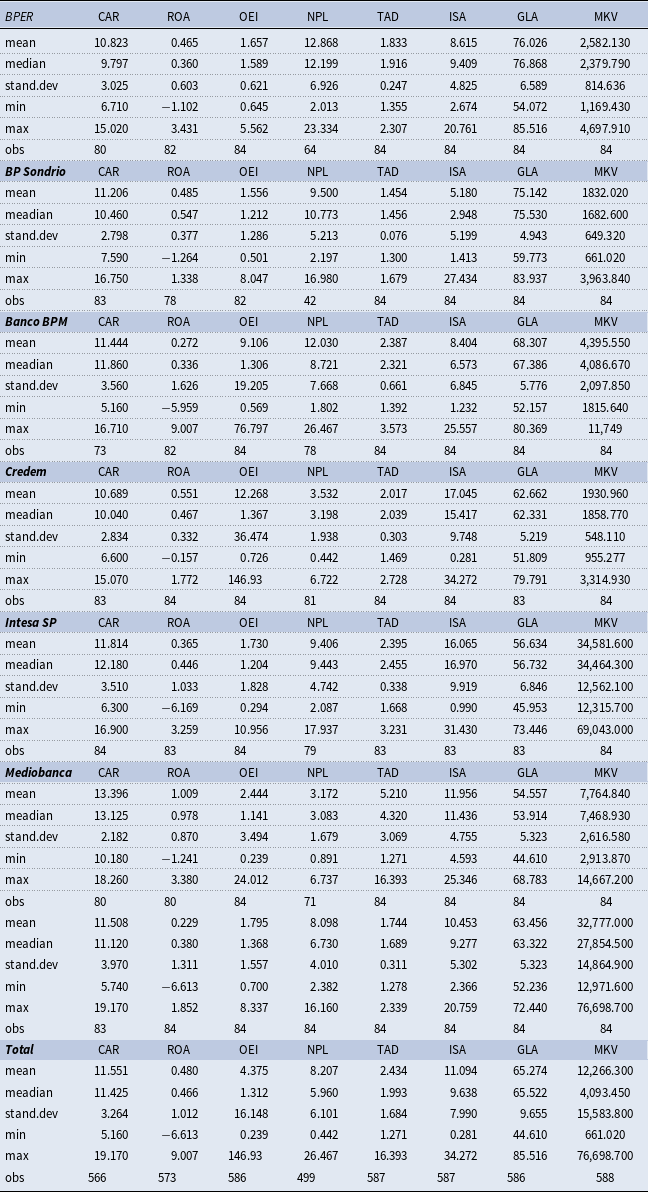
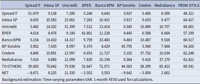


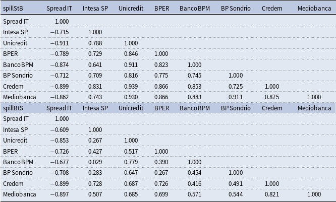
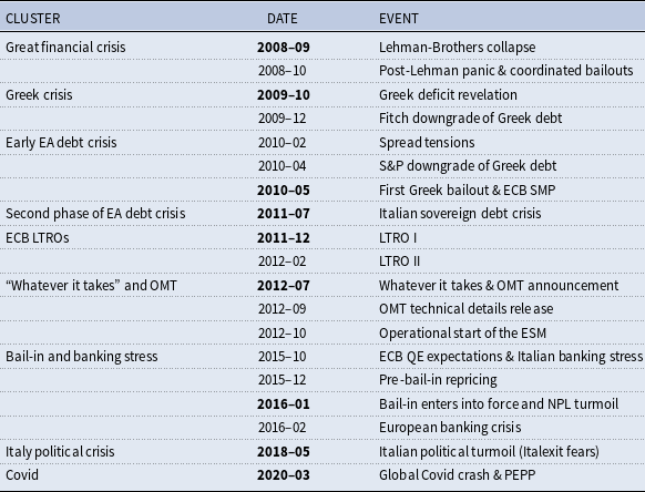
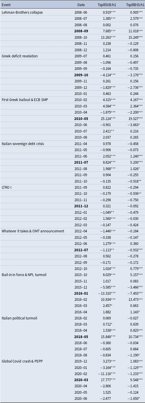
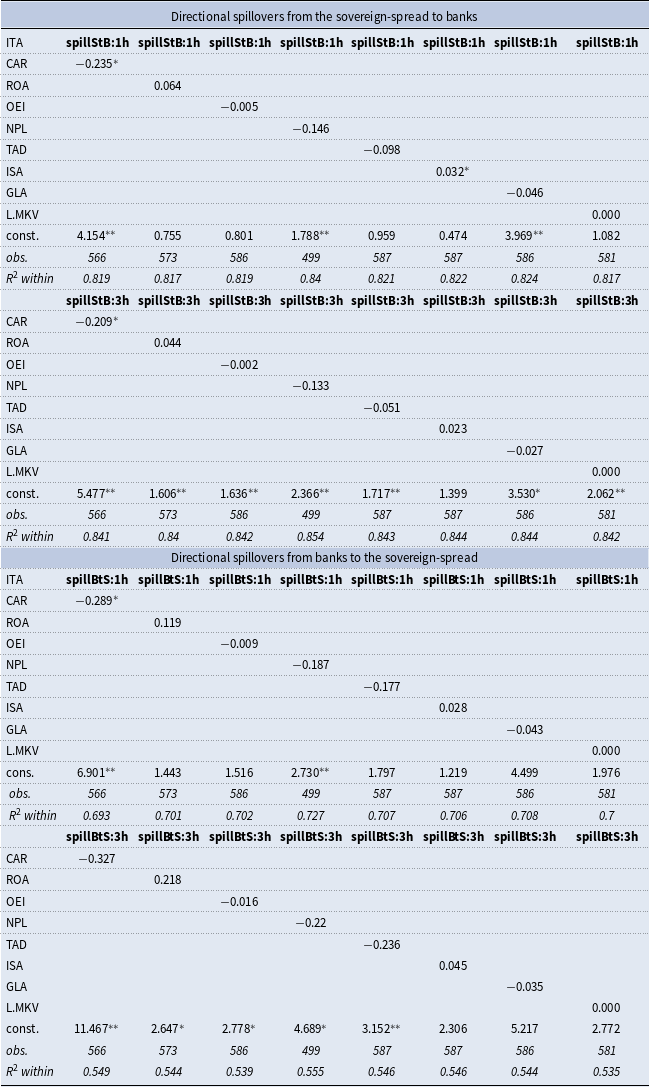
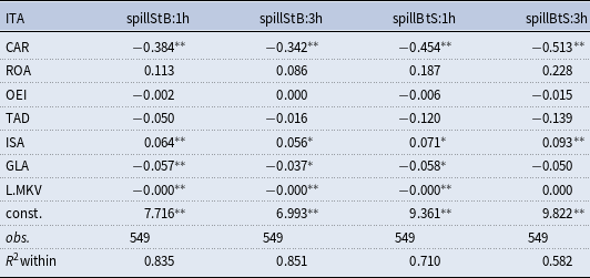

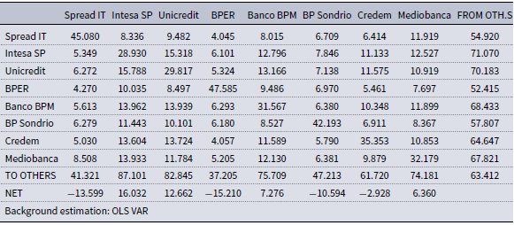

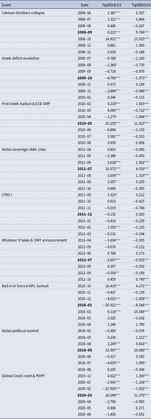
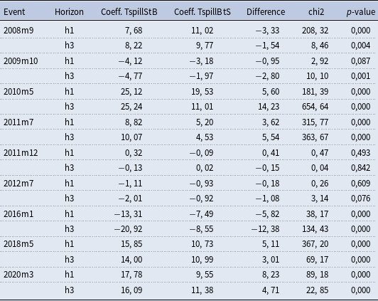
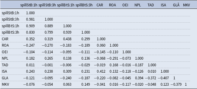
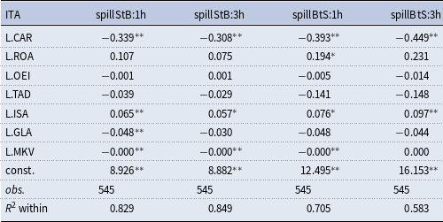
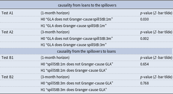

 Open access

