INTRODUCTION
The notion that sectoral productivity shocks underlie the flow of labor from one industry, producer, or region to another is a well-established idea in both the macroeconomics and labor literatures.1
Examples include (among many others) Campbell and Fisher (2000), Davis and Haltiwanger (1999a, 1999b), Caballero et al. (1997), Davis et al. (1996), Caballero and Hammour (1994), Mortensen and Pissarides (1994), Loungani and Rogerson (1989), and Lilien (1982).
To be fair, there is a large empirical literature linking productivity growth to job flows [see, for example, Davis and Haltiwanger (1999b, pp. 2762–2768) for a survey]. Overwhelmingly, however, these studies [e.g. Baily et al. (1992), Baily et al. (1996), Foster et al. (1998)] approach the issue by conducting decompositions of aggregate productivity growth into components accounted for by plants belonging to various categories—for example, expanding (including entering) establishments as opposed to contracting (including exiting) ones. This paper, by contrast, seeks to estimate the direct effects of job creation and destruction on productivity growth, accounting for their joint determination.
There is certainly ample reason to believe that they do. After all, much of the literature studying the determinants of job creation and destruction posit that, in response to some underlying shock (either technology- or demand-related), workers are reallocated across production units. This reallocation, in turn, affects the cross-sectional distribution of productivity across individual workers and producers and, thus, the aggregate productivity they engender.
Although there is some disagreement over the basic mechanisms underlying job destruction, there is a reasonably broad consensus regarding its conjectured impact on aggregate productivity. To be sure, virtually all studies suggest that job destruction takes place primarily among the most inefficient production arrangements in any given cross-section. Merz (1999) and Den Haan et al. (2000), for example, examine models in which producers eliminate jobs in response to negative shocks to firm-worker “match quality.” Caballero and Hammour (1994) study an environment in which decreases in the demand for an industry's output result in the elimination of the most inefficient production units in operation. In each of these instances, the act of destroying jobs serves to increase aggregate productivity by removing the bottom end of the micro-level productivity distribution.
Empirically, this rather straightforward conjecture has a fair amount of support. For example, in the context of firms, Baily et al. (1992), Griliches and Regev (1995), and Olley and Pakes (1996) have found that low productivity does indeed predict a producer's exit from the market. Evidence on the nature of job destruction implied by studies of individual work histories suggests a similar conclusion. Gibbons and Katz (1991), for instance, report that firms tend to target workers from the low end of the productivity distribution for layoffs when reducing total employment. Farber (1993) finds that, between 1982 and 1991, rates of job loss were higher among younger, less educated workers than among older, more educated ones.
The nature of job creation and its impact on productivity, by contrast, is somewhat less clear-cut. Some papers [e.g., Caballero and Hammour (1994), Mortensen and Pissarides (1994), and Hall (2000)] suggest that job creation represents the allocation of workers into new, technologically advanced (and, thus, high-productivity) work arrangements. When combined with the characterization of job destruction described earlier, this line of reasoning suggests that, overall, job flows can be viewed as a manifestation of “creative destruction.”
Evidence on this particular hypothesis, however, is somewhat mixed. Although studies such as Baily et al. (1992) and Foster et al. (1998) find that the reallocation of workers from low- to high-productivity establishments contributes positively to aggregate productivity growth in U.S. manufacturing, Bowlus (1995) and Barlevy (2000) find that, on the whole, workers do not move into more productive positions during recessions, when rates of job destruction (thus, presumably, rates of productive reallocation) are especially high. Consequently, the extent to which job creation involves additions to the upper end of the job-productivity distribution remains uncertain.
In fact, other studies have taken a very different view of the matter, suggesting that job creation may, instead, reduce aggregate productivity. Merz (1999), for instance, explores an environment in which employment variation occurs primarily along a low match-quality margin. That is, when firms experience positive productivity shocks, they expand their employment by hiring predominantly low-wage (i.e., low-productivity) workers, whereas, given negative shocks to productivity, employment falls as these very same workers are laid off. In such an instance, because job creation involves the expansion of the lower tail of the worker productivity distribution, it confers a negative effect on aggregate efficiency.
Evidence reported by Solon et al. (1994), interestingly, is broadly consistent with this characterization of the labor market. Using data from the PSID, they find that the contribution of low-wage labor exhibits greater variation over the business cycle than high-wage labor. Thus, during recessions, low-wage workers are laid off in greater numbers than high-wage workers, whereas in expansionary periods, greater numbers of low-wage workers are hired. Assuming that low wages are indicative of low productivity, this evidence suggests that, by itself, job creation should reduce aggregate efficiency.
This paper attempts to evaluate these competing views of job flows by estimating the impact of job creation and job destruction on the growth of total factor productivity (TFP) using annual data on more than 300 four-digit manufacturing industries in the United States over the period 1974–1993. As a brief summary of the results, I find that, consistent with the consensus view, job destruction does indeed have a positive influence on TFP growth. Thus, on average, there certainly appears to be a cleansing aspect to the job-destruction process. However, contrary to the pure creative-destruction view, I also find that job creation tends to have a negative influence on productivity growth. On balance, then, the evidence favors the view that, on the whole, job creation and destruction represent employment changes along a predominantly low-skill/low-productivity margin rather than productive reallocation.
A more detailed look at the effects of job creation and destruction within continuing plants as opposed to the effects of plant births and deaths using two-digit data generates a similar conclusion. Although the results do not provide complete support for either theory, they do tend to be more consistent with the match-quality view of job flows than the pure creative destruction notion.
The remainder of the paper proceeds as follows. Section 2 presents a simple theoretical framework used to derive the hypothesized statistical relationship between job flows and TFP growth. The data and results from formal estimation of this relationship are then discussed in, respectively, Sections 3 and 4. Section 5 concludes.
THEORETICAL CHARACTERIZATIONS OF TFP AND JOB FLOWS
This section develops a simple framework to explore the connection between job flows and total factor productivity growth. As noted earlier, two general approaches have been taken when examining this nexus. The first—the “job match-quality” view [e.g., Merz (1999)]—suggests that both employment gains and losses involve jobs primarily situated at the bottom end of the productivity distribution. The second—the “vintage capital” approach [e.g., Caballero and Hammour (1994)]—views job creation and destruction as the means by which unproductive work arrangements are replaced by more productive ones. I consider each in turn.
Job Match Quality
Consider an economy comprised of many producers/firms, indexed by j, each of which belongs to an industry, indexed by i. In order to operate in any given time period t, a producer hires some number Nj,i,t>0 of workers (the determination of which is described below) from a pool of available labor. Once assembled, this labor force then generates output, Yj,i,t, given by:

where θj,i,t>0 denotes a producer-specific random technology shock, Kj,i,t>0 is the producer's endowment of physical capital,
is worker w's labor input, and
is worker w's time-invariant index of productivity (or match quality), all at time t. For the sake of simplicity, suppose that the producer's stock of physical capital is constant and that all workers supply the same quantity of labor input, L, inelastically at each point in time.3
Note, these particular assumptions are not crucial since the ultimate object of interest, TFP, takes into account the effects of observable inputs (e.g., capital and labor hours) on output.
Notice, although workers supply the same quantity of labor when hired, they do not all contribute equally to production. In particular, heterogeneity in the match-quality parameters, A—which, in practice, may derive from any of a host of individual characteristics including education, experience, or innate ability with respect to a particular job—implies that some workers are, quite simply, more productive than others. Because I am abstracting from labor market search decisions, I assume that these parameters are perfectly observable so that the producer knows the exact distribution of worker productivities when assembling a labor force. I also assume that the producer may hire any worker that it wants. The producer's problem, then, reduces to the choice of an optimal number of workers to hire at each point in time. To solve such a problem, consider first the specification of payoffs.
Workers in this framework are paid their marginal products, so that, in aggregate, labor receives (1−α)Yj,i,t in each time period t. The producer, who owns the stock of physical capital, K, then receives the remainder, αYj,i,t.4
This payoff scheme is analogous to a Nash bargaining solution, which is common in matching models [e.g., Acemoglu (1996); Den Haan et al. (2000)]. The results derived here hold for general firm-worker splits given by shares π and 1−π, π∈(0, 1).

where g′>0 and g″>0. This second term, g(Nj,i,t), is designed to capture the cost that a producer must, for instance, pay a manager to ensure that production proceeds smoothly. The fact that it is strictly increasing and convex in the number of workers hired reflects the notion that coordination becomes increasingly difficult as more and more workers are assembled [e.g., Williamson (1967); Becker and Murphy (1992)].5
The addition of the coordination cost also makes the producer's problem well defined. Without it, optimal employment and the producer's payoff are both infinite.
The producer's problem, then, consists of choosing Nj,i,t to maximize (2) conditional on knowledge of the technology shock, θj,i,t. Doing so is straightforward. First, notice that the producer will always employ the most productive workers in the economy: for a given Nj,i,t, αYj,i,t strictly increases in the productivity index of each worker hired whereas the coordination cost is constant. As a result, when evaluating the payoff associated with a particular level of employment, Nj,i,t, the producer simply substitutes the Nj,i,t highest values of A into (2). Optimal employment is then given by the value of Nj,i,t that generates the highest quantity.
Based on this setup, we have the following intuitive result linking technology shocks and the producer's optimal employment.
PROPOSITION. Optimal employment is nondecreasing in θ.
Proof. The term αYj,i,t is strictly increasing in the number of workers hired. Therefore, the amount by which an increase in the technology term, θj,i,t, increases αYj,i,t increases in the number of workers hired. As such, the increase in the difference αYj,i,t−g(Nj,i,t) in response to a rise in θj,i,t also increases in Nj,i,t, which implies that the optimal value of Nj,i,t cannot decrease in response to a positive technology shock.
Hence, as producers receive technology shocks, θ, the overall productivity of each worker's match, θA(w), changes, thus inducing potential changes in optimal employment.
Given that the most productive workers in the economy are employed at each point in time, changes in employment are accomplished by altering the number of relatively low match-quality jobs in operation. Thus, in response to a negative technology shock, which reduces optimal employment by, say, P employees, a producer simply eliminates the P least productive matches.
The timing of the shock process and the producer's employment adjustment take the following form. At the beginning of each period, the technology shock is realized, implying an optimal employment level. Over the remainder of the period, the producer begins adjusting employment to meet this optimal level, which may take one or more periods to attain. The presence of certain labor market rigidities, such as contracts requiring producers to give workers notice that they will be fired (given a negative shock) or, if one allows for search considerations, finding and hiring workers that are desired (given a positive shock) may require producers to adjust employment only gradually.6
Note, gradual adjustment would be consistent with the evidence reported by Stevens (1997), who finds that displaced workers suffer significant earnings losses in both the year before and year of displacement.
From this basic characterization of employment and production, producer j's total factor productivity (TFP) can be expressed as follows:

That is, a firm's TFP is calculated by dividing output by the measured capital input, which, conditional on knowledge of α, is just Kα and the measured labor input, which is given by Nj,i,tL1−α (Nj,i,t workers, each of whom supplies L units of labor).7
In formulating this expression for TFP, I assume that the match-quality parameters are not observed and, thus, are not accounted for by the researcher who calculates TFP. Although the distinction between production and nonproduction workers is accounted for in the TFP measure considered here (see Section 3.1), no other labor-quality adjustments are made.

where
.
Because the change in the average match quality over all workers within a firm depends directly on the extent to which the firm is expanding or contracting the number of workers that it employs (employment gains reduce
, employment losses raise
), TFP growth can be reformulated in terms of rates of job creation, POS, and job destruction, NEG:

where the parameters γC<0 and γD>0 represent the influence of creation and destruction on productivity growth. Note, because producers either expand or contract (or neither), only one of the terms, POSj,i,t or NEGj,i,t can be nonzero at a given point in time.
Now, because industry aggregates are merely weighted sums of firm-level measures, industry i's productivity growth follows as:

where ωj,i,t denotes producer j's weight in the industry at t. This expression, of course, can then be written more compactly in terms of industry-level technology growth, job creation, and job destruction:

Vintage Capital
A second line of inquiry suggests that job flows embody creative destruction. That is, simultaneous job creation and destruction act as a mechanism by which inefficient production units are eliminated and more efficient ones established. This idea has been formalized, for example, by Caballero and Hammour (1994), who demonstrate that such a process can explain, among other things, the asymmetric patterns witnessed in the creation and destruction series.
The fundamental idea of that paper can be applied to a setting analogous to the one sketched above in the following manner. Let production of firm j of industry i at time t, Yj,i,t, be given by the product of an efficiency term (TFP), θj,i,t, and some function of a fixed amount of labor and capital. On isolating each producer's index of efficiency, the logarithm of industry i's TFP can be approximated as a weighted sum over its constituent firm-level measures:

where, as before, ωj,i,t is plant j's weight in the industry in period t, and Ωt is the set of plants in operation during this period. Industry-level TFP growth then follows as:

which can be rewritten in a manner analogous to the decomposition considered by Baily et al. (1992):

Notice, the first term in this expression represents the change in the weighted log-productivity sum taken across continuing plants (i.e., those in operation at both t−1 and t); the second, the weighted log-productivity sum over plants entering at t, who (by assumption) utilize the most efficient technologies available; the third, the weighted log-productivity sum across plants exiting the market after period t−1, who (again, by assumption) utilize the least efficient technologies.
Given that all firms in operation employ a constant amount of labor, job creation and destruction in this framework are merely the products of entry and exit. Thus, the three terms on the right-hand- side of (10) can be expressed in a manner analogous to (7):

The underlying source of job flows in Caballero and Hammour's (1994) model, other than purely exogenous rates of technological progress and producer obsolescence, are demand shocks. Increases in the demand for an industry's output result in decreases in the rate at which low-productivity producers are eliminated (as greater numbers of producers are required to accomodate the rise in demand), whereas decreases in demand do just the reverse. Although the magnitude of the response is somewhat smaller, demand shocks have the opposite effect on job creation. Positive (negative) shocks are met with modest increases (decreases) in the rate at which new production units are established.8
For a rigorous characterization of the response of job creation and destruction to demand shocks, see Caballero and Hammour (1994).
More important, consider the influence of job creation and destruction on TFP growth. Job creation in this formulation is clearly a benefit to industry productivity. As new producers are added, a larger share of industry output is accounted for by higher productivity plants. Hence, γC>0. Job destruction, by contrast, also serves a beneficial role as it represents the elimination of the most inefficient producers. Thus, because high rates of destruction also increase the weights assigned to the most efficient producers, γD>0 as well.
Notice, although these particular implications regarding the direct effects of job flows on productivity are straightforward, evaluating the overall effect of a demand shock on an industry's rate of TFP growth is more complicated. That is, whether a positive shock to demand (say, associated with an expansionary period) generates greater or lower productivity growth is not clear-cut. A rise in demand, for instance, may be associated with more job creation but less job destruction, thereby leaving the overall change in TFP ambiguous. Moreover, although the TFP of each continuing plant does not change in Caballero and Hammour's (1994) formulation, permitting it to do so would further complicate the change in productivity emanating from a change in demand.9
Hence, as they carefully note (p. 1365), this formulation does not necessarily imply a particular cyclical pattern for productivity with respect to expansions and recessions.
DATA AND STATISTICAL METHODS
Productivity and Job-Flow Data
The productivity data used in the analysis are taken from the NBER Manufacturing Productivity Database (MPD), which reports annual rates of TFP growth for roughly 450 four-digit industries between 1958 and 1996. The job-creation and destruction data, which are defined as total employment gains and losses, respectively, expressed as percentages of total industry employment, are reported by Davis et al. (1996) over the period 1973 to 1993.10
John Haltiwanger has generously provided these data online at http://www.bsos.umd.edu/econ/haltiwanger.
Because the standard industrial classification (SIC) scheme changed in 1987, I consider two sample time frames. First, I look at the period 1974 to 1993 using 337 industries whose compositions did not change with the SIC revision.11
This is accomplished using the correspondence between the two systems provided by the NBER. I use only those industries whose 1987 composition matches completely with the 1972 composition (i.e., the 1972–1987 and 1987–1972 shares both equal 1). I begin the series at 1974 because the instrumental variables employed in the analysis below begin in 1974.
Two measures of TFP growth are reported by the MPD: a five-factor growth rate (capital, production worker hours, nonproduction workers, nonenergy materials, and energy) and a four-factor growth rate (energy and nonenergy materials are not treated separately).12
For further information about the MPD, see Bartelsman and Gray (1996).
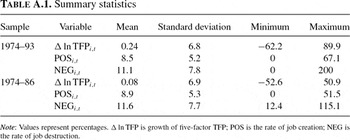
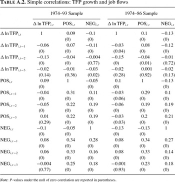
Several basic properties of the data deserve some mention. First, the contemporaneous correlation between job creation and job destruction across four-digit industries is only weakly negative, −0.05 (1974–93) and −0.13 (1974–86). These figures stand in contrast to the one reported by Davis et al. (1996, p. 33) for aggregate manufacturing over the period 1973–1988, −0.75, and to the correlations of the employment-share weighted averages of job creation and destruction in the present samples, −0.63 (1974–1993) and −0.74 (1974–1986). This result seems to suggest that simultaneous increases or decreases in creation and destruction occur more frequently within four-digit industries than within aggregate manufacturing itself. It also indicates that, at this level of aggregation, these two series are relatively independent. Both may, therefore, enter feasibly into a single regression equation.13
That is, identifying the separate effects of creation and destruction on productivity growth should not be impaired by an excessively high degree of collinearity between them.
Second, TFP growth is positively correlated with contemporaneous job creation (POS) but negatively correlated with contemporaneous job destruction (NEG). This feature, of course, can be interpreted in terms of both hypotheses discussed earlier. Positive technology shocks, for instance, may induce producers to expand their payrolls, thus generating an increase in both creation and TFP growth. Similarly, a rise in demand may induce greater job creation, which, in turn, may raise overall productivity as especially productive jobs are established. Although, in both cases, job destruction would decrease, thereby mitigating any increase in productivity growth, it is certainly possible to observe productivity growth moving (on average) with creation but against destruction.
Third, just as Baily et al. (1992) find among individual manufacturing establishments, TFP growth at the four-digit industry level is significantly, negatively autocorrelated. Although Baily et al. (1992) suggest that this mean-reverting tendency can be interpreted in terms of a model in which there are random shocks to productivity levels (i.e., higher-than-average shocks in one period tend to be followed by smaller shocks subsequently), it should be noted that it is also compatible with the job-matching formulation above with persistent shocks to technology.
Suppose that, given a negative technology shock at t, which persists for two periods, producer j adjusts its employment to the new (lower) optimal level in periods t and t+1. Again, various labor market rigidities may necessitate a gradual transition of employment levels over time. In period t, there would be a negative contemporaneous correlation between TFP growth and job destruction as long as the initial decrease in θj,i,t outweighed the increase in the average match quality
as low productivity workers are released. In the following period, however, as job destruction continues, TFP will begin rising.14
The fact that each job-flow series is positively autocorrelated (see Table A2) is certainly compatible with the notion of persistent shocks and gradual adjustment.
For such a scenario to be plausible, naturally, TFP growth and job destruction would have to move together in some periods, whereas TFP growth and job creation would have to move in opposite directions some of the time. As it turns out, the data indicate that both happen roughly half of the time. Using both samples (1974–1993 and 1974–1986) of observations on {Δ ln TFPi,t−Δ ln TFPi,t−1}, {POSi,t−POSi,t−1}, and {NEGi,t−NEGi,t−1}, I find that TFP growth and the rate of job destruction either both increase or decrease roughly 46 percent of the time. TFP growth and job creation move in opposite directions in about 46 percent of the observations.15
Although they study labor productivity, these findings are similar to those of Baily et al. (1996, p. 267), who find that over half of all expanding plants experience productivity declines, whereas over half of all contracting plants experience productivity increases.
In terms of the implied correlations, this example suggests that the contemporaneous correlation between job creation and TFP growth as well as that between job destruction and TFP growth will be given by a mixture of positive and negative values. As mentioned earlier, on net, such a correlation could very well be positive for job creation and negative for job destruction (as in the data). At one lag, however, the implied relationships in this particular instance are clear: job creation (destruction) will be positively (negatively) correlated with lagged TFP growth, whereas TFP growth will be negatively (positively) associated with lagged job creation (destruction). All, as it happens, are borne out empirically.
What is more, TFP growth itself will be negatively autocorrelated as a direct consequence of the job flows that are induced by the underlying (persistent) technology shocks: productivity gains induce job creation, which generates future losses; productivity losses induce job destruction, which generates future gains. Thus, random shocks—as in Baily et al. (1992)—are not necessary for mean reversion.16
Indeed, one also could rationalize mean reversion in TFP growth with persistence in the growth rate of technology, Δ ln θ, as long as job creation and destruction adjust slowly (i.e., an increase in technology growth at t, which persists through t+1, induces a small increase in creation at t but a large increase at t+1).
Although intriguing, none of these casual statistics provide any direct evidence on how either job-flow series influences TFP growth. Hence, at this point, I turn to the formal estimation of the models sketched earlier.
Statistical Model
The theoretical characterization of productivity growth derived in Section 2,

provides the basis for the statistical analysis that follows. I begin by specifying the structure of the average technology growth term Δ ln θi,t as a stationary AR(P) process, designed to capture any autocorrelation in the underlying shocks (i.e., technology or demand shifts):

where the term ξi,t is the sum of two elements: an overall constant, μ, and a white-noise term specific to industry i at time t, εi,t.17
It should be noted that if ln θi,t follows a stationary autoregression in levels, this representation in differences will involve an MA(1) error instead of white noise. However, because none of the estimated specifications reported in Tables 1–3 produced residuals with significant first-order autocorrelation, I proceed under the assumption that (11) is valid.

where L denotes the lag operator, so that the equation describing TFP growth earlier becomes:

So, for example, an AR(1) representation of the technology process results in the following specification:

which involves the estimation of four parameters: μ, ρ1, γC, and γD.
The difficulty associated with estimating this equation, of course, is the endogeneity of the contemporaneous job-flow terms, POSi,t and NEGi,t. Based on the job match-quality formulation, for example, an increase in εi,t signifies a positive shock to (average) industry productivity. Although this shock increases TFP, it also affects the extent to which firms are creating and destroying jobs because εi,t is itself the sum of firm-level technology terms that determine employment changes. Similarly, a shock to demand in the vintage capital formulation influences both the extent of job creation and destruction as well as the term εi,t through its influence on the weights ωj,i,t of the continuing plants. A negative demand shock, for instance, may decrease creation and increase destruction and, simultaneously, increase the weighted average productivity over continuing plants. Simple nonlinear least squares (NLLS) estimation of (13) would, therefore, generate biased estimates of the creation and destruction effects, γC and γD.18
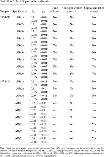
For the purpose of comparison, NLLS estimates of the creation and destruction parameters for each of the specifications considered below appear in Table A.5 of the Appendix.
Consequently, to estimate (13), I turn to the use of instrumental variables. As instruments for the two endogenous job-flow series, I utilize three variables describing an industry's plant-size distribution: the logarithm of the average number of workers per plant, the percentage of all establishments with at least 500 employees, and the percentage of all establishments with fewer than 50 employees, all lagged one period. Hence, these three “average plant-scale” variables at time t instrument for an industry's job creation and destruction between t and t+1.
Annual data on establishment counts by employment size categories for four-digit manufacturing is taken from annual County Business Patterns (CBP) files produced by the Bureau of the Census. From these data, the percentage of plants employing fewer than 50 employees and those employing 500 or more are readily computed.19
The size categories (in terms of employees) reported in the U.S. summary data files include the following: 1–4, 5–9, 10–19, 20–49, 50–99, 100–249, 250–499, 500–999, 1,000 or more. Casual experimentation indicated that the proportions of establishments situated in the (combined) 1–49 and 500 or more groupings were particularly correlated with creation and destruction.
Are these variables plausible as instruments for the two job-flow series? Instrumental variables, of course, must satisfy two criteria. First, they must be exogenous with respect to, in this case, total factor productivity growth. Second, they must be correlated with job creation and destruction.
To begin, lagged features of an industry's establishment size distribution are certainly not determined by subsequent productivity growth. Hence, there are no simultaneity problems associated with these variables. Moreover, existing studies of plant-level productivity indicate that lagged establishment size characteristics are themselves unlikely to be the central determinants of TFP growth. Baily et al. (1992), for example, find that plant size—measured by total employment—is not a significant predictor of TFP growth in their sample of manufacturing establishments. Foster et al. (1998, pp. 10–11) offer a similar conclusion in their survey of the literature studying plant-level productivity, noting that, although productivity levels tend to be higher in large establishments, “it has been more difficult to find correlates of changes in productivity.”20
For example, they note that although Dunne (1994) finds that large plants are more likely to adopt “advanced” technologies (e.g., CAD/CAM), which may help to rationalize their high productivity levels, Doms et al. (1997) find that the growth of average labor productivity is only weakly connected to the adoption of these technologies.
In the data used here, the raw correlations of TFP growth with the logarithm of average plant size, percentage of plants with at least 500 workers, and percentage with fewer than 50 workers (all lagged one period) are small: −0.03, −0.02, and 0.02 (1974–93); −0.02, −0.01, 0.01 (1974–86). Only the first of these values (average employment in the 1974–1993 sample) differs statistically from zero at 10% significance.
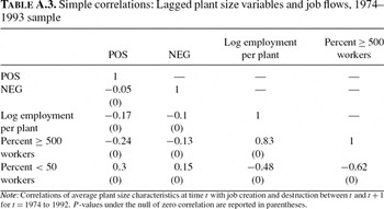
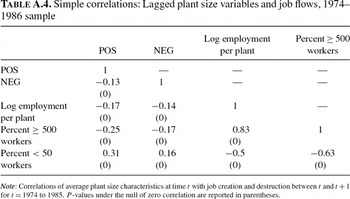
At the same time, measures of average establishment size tend to be highly correlated with rates of job creation and destruction. Davis et al. (1996), for instance, document a strong inverse association between average establishment size—measured directly by employment as well as indirectly through average wage earnings and capital intensity—and both job-flow series. A similar result is shown in Tables A3 and A4 of the Appendix, which report correlations between creation and destruction rates and each of the three lagged plant-scale variables among the industries considered here. Clearly, as industries organize their activity around establishments with greater numbers of employees, average rates of job creation and destruction fall dramatically.
RESULTS
Baseline Estimates
Estimation of (13) is performed in two ways: (nonlinear) two-stage least squares (2SLS) and generalized method-of-moments (GMM).22
This discussion follows Chapters 10 and 11 of Greene (2000).

where ε(·) is an (n×1) vector of residuals associated with parameter vector β, Z is an (n×g) matrix of instrumental variables, n is the number of (industry-year) observations, and g the number of instruments (here, equal to three). GMM, by contrast, selects the vector of parameters to solve a similar, but slightly more general minimization problem:

Here, Σ is an (n×n) covariance matrix of the error terms, εi,t, and (Z′ΣZ) represents the estimated (g×g) covariance matrix of the model's moment conditions Z′ε(β), scaled by n2.
These two objective functions, of course, coincide when Σ is some scalar multiple of the identity matrix—that is, when the errors are mutually uncorrelated and homoskedastic. In practice, however, because I base the GMM estimates on a heteroskedasticity-consistent specification of Σ, they will generally differ from the 2SLS estimates.23
The specification of the error matrix follows that of White (1980), so that (Z′ΣZ) in (16) is estimated as
, where zi is the (g×1) vector of instruments for observation i.
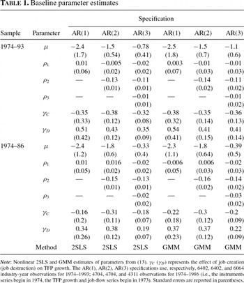
Results for each of three lag lengths describing Δ ln θi,t—AR(1), AR(2), AR(3)—appear in Table 1. Two features are particularly noteworthy. First, many of the estimated autoregressive parameters, ρ, are negative (particularly at two lags), implying that the shock process, Δ ln θi,t (i.e., the “residual” element of TFP growth after removing the effects of job creation and destruction) follows an autocorrelation pattern similar to one characterizing the raw productivity growth levels (Table A2). Although not completely surprising, this result does offer some evidence on the role of employment variation in generating a mean-reverting TFP growth series. In particular, although job creation and destruction may certainly contribute to a negative autocorrelation pattern in productivity growth (as described in Section 3.1), the evidence does not support the idea that job flows themselves provide a complete explanation for this pattern. Independent of the effects of job creation and destruction, TFP growth is negatively autocorrelated.


Second, the estimates reveal a positive influence of job destruction, although a negative influence of job creation, on TFP growth. Statistically, in fact, the majority of the relationships are significant: of the twelve coefficients reported for each sample, only the parameters from the AR(1) specifications are indistinguishable from zero at conventional significance levels. Moreover, the magnitudes of the coefficients also suggest economically significant effects. Based on the point estimates, a 1 standard-deviation increase in job destruction (roughly eight percentage points), for example, is accompanied by a 1.5 to 4 percentage-point increase in TFP growth, on average, whereas a 1 standard-deviation rise in job creation (approximately five percentage points) is associated with one to two percentage-point decrease in TFP growth. Given that the overall standard deviation of the TFP growth series is about 7% in either sample, these estimated effects are substantial.
Of course, one reason for these large magnitudes may be that this first specification of the model does not account for the potential influence of exogenous time effects on productivity growth. In particular, if they are correlated with the two job-flow series, the creation and destruction parameters given in Table 1 may simply be reflecting the influence of these time effects.
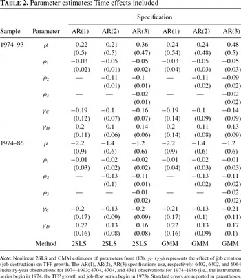
To examine this possibility, I estimate (13) with year dummies included. The resulting parameter estimates appear in Table 2. Notice, although the coefficients in this case are now somewhat smaller—the estimated effects of a 1 standard-deviation change fall between 0.7 and 1.5 percentage points for destruction, 0.5 and 1 percentage points for creation—and, unfortunately, not as consistently significant across all specifications, they still suggest the same qualitative pattern. Job creation serves to reduce productivity growth, job destruction acts to boost it. Given the two characterizations of the job flows-productivity growth nexus described earlier, then, this baseline evidence tends to favor the job-matching perspective over the vintage capital view.24
These results also may offer some insight into why the observed association between establishment size and TFP growth tends to be weak in studies of plant-level data [e.g., Baily et al. (1992)]. Large plants tend to experience lower rates of job destruction (hence slower productivity growth) as well as job creation (hence faster productivity growth). Given a cross-section of expanding and shrinking plants, little overall correlation may emerge between size and productivity growth. This mechanism also would imply that the dispersion of productivity growth is higher in smaller plants (due to higher job-flow rates), which is broadly consistent with the evidence reported by Dunne et al. (1989).
Robustness: Factor Utilization and Intensity
Empirically, TFP has proved to be an elusive concept due to the likely influence of unobserved inputs on measured output. In particular, variations in factor utilization have been shown to play a large role in the dynamic properties of Solow-residual type measures of technological progress, such as those reported in the MPD [e.g., Burnside et al. (1993) and Shapiro (1993)]. Furthermore, because factor utilization is largely unobservable, this concern has plagued studies of productivity dynamics for years.
A recent paper by Basu and Kimball (1997), however, suggests a simple correction that can be performed to account for variable capital and labor utilization. Assuming that firms are cost minimizers and price takers in factor markets and that the only cost of increasing the work-week of capital is the compensation of workers for a shift premium, changes in hours per worker can be used to proxy for changes in the utilization of both capital and labor.25
Basu and Kimball (1997) find that allowing for increased capital utilization to generate a second cost, faster depreciation, does not greatly alter their productivity calculations.
Additionally, Klenow (1998) finds that rates of total factor productivity growth vary significantly with respect to capital and labor intensity. Specifically, capital intensive industries seem to experience faster rates of TFP growth than labor-intensive ones, at least over fairly long time horizons. As a consequence, some correction for the extent of capital and labor intensity across industries may be required.
Following these observations, I include as exogenous regressors into (13) the contemporaneous values of the growth rate of hours per worker among production workers, the share of capital in total output, and the share of labor in total output. These shares are calculated as in Klenow (1998), who defines an industry's labor share as its total payroll divided by its total value of shipments, materials share as total materials cost (including energy) divided by the total value of shipments, and capital share as the residual after subtracting these first two from unity.
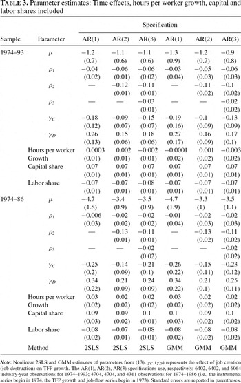
The resulting parameter estimates appear in Table 3. Beginning with the three correction terms, we can see that hours per worker growth appears to play little role, at least after having conditioned on all other variables appearing in the model. Capital and labor shares, by contrast, do enter significantly and [following Klenow's (1998) evidence] with the expected signs: industries with greater capital intensity tend to experience faster TFP growth; those with greater labor intensity tend to experience slower growth.

As for the remainder of the parameters, the estimated values are similar to those reported in Tables 1 and 2. The autoregressive coefficients, for instance, remain negative and display the same pattern with a particularly strong AR(2) term. More important, the job-destruction and creation parameters remain, respectively, positive and negative, exhibiting roughly the same magnitudes as those from Table 2. Although not all of the coefficient estimates are significant in this case (e.g., only one of the job-creation terms, γC, differs statistically from zero at conventional levels in the 1974–1993 sample, two in the 1974–1986 sample), the results certainly appear to reinforce the basic conclusion drawn earlier.
It is worthwhile at this point to compare these instrumental-variables (IV) estimates of the effects of job creation and destruction, given in Tables 1–3, with those derived from the estimation of (13) by nonlinear least squares (NLLS), which are summarized in Table A5 of the Appendix. Looking at the two sets of estimates, the differences are striking. In particular, based on the NLLS coefficients, job creation appears to have a positive impact on TFP growth, whereas job destruction has an apparently detrimental effect.
To the extent that one trusts the 2SLS and GMM results, naturally, this distinction suggests that contemporaneous creation and destruction are, respectively, positively and negatively associated with the stochastic error term. That is, only a positive association between POSi,t and εi,t could produce a positive estimate for a truly negative coefficient (γC), whereas a negative association between NEGi,t and εi,t generates a negative estimate for a truly positive coefficient (γD). Given the two characterizations of job flows and productivity growth sketched earlier, the job-matching framework, I hold, better accounts for this conjectured correlation structure.
Indeed, following the framework of Section 2.1, a positive shock to industry i's average TFP growth (i.e., a rise in εi,t) will generate an increase in contemporaneous job creation, whereas contemporaneous job destruction falls. Hence, the job match-quality formulation implies that NLLS estimate of γC (γD) will be positively (negatively) biased.
The vintage capital notion, by contrast, is somewhat more difficult to reconcile with this presumed correlation pattern. Consider, for example, a negative shock to industry i's demand. Because overall demand is now lower, the extent of job creation should fall, whereas the amount of job destruction should rise. This process, in turn, increases the average TFP taken over continuing establishments, θi,t, because a higher rate of destruction eliminates a larger part of the bottom end of the plant-level productivity distribution. Interpreting this result as an increase in the stochastic term εi,t, the resulting correlations with creation and destruction are, respectively, negative and positive. In such an instance, the IV estimates would possess the same signs as those of the NLLS estimates.
Job Flows in Continuing Plants versus Births and Deaths
One difficulty involved with the interpretation of these results in the context of the job matching and vintage capital theories stems from the fact that these two explanations are targeted at fundamentally different aspects of the creation and destruction process. As described in Section 2, the former involves the variation of employment within continuing establishments, whereas the latter characterizes job flows in terms of entry and exit. Because the data used thus far quantify aggregate job flows—that is, those involving contributions from continuing establishments as well as the influence of births and deaths—the results reported above reflect some average effect across these underlying pieces.
Furthermore, because the majority of employment gains and losses in U.S. manufacturing take place among continuing plants [Davis et al. (1996)], it is logical that the evidence would favor the job-matching framework. As such, the results do not necessarily imply that the vintage capital view of job creation and destruction is invalid. Indeed, it may simply be that, in these aggregate data, the positive effect associated with plant births is outweighed by the negative effect of creation among stayers. In order to explore this possibility, however, data in which creation and destruction have been decomposed into different types (i.e., continuing versus births and deaths) would be required.
Although this information is not available at the four-digit level in the Davis et al. (1996) data, it is available at the two-digit level. Hence, I can provide at least a cursory look at any potential differences in how different types of job creation and destruction influence productivity growth among this coarser grouping of industries. To do so, I consider the following simple exercise. Using 19 sectors26
The data of Davis et al. (1996) combine SIC 20 (Food and Kindred) and SIC 21 (Tobacco) for the vast majority of years. In the analysis, I treat these combined industries as a single sector.
Although strong, the correlations between the two types of creation, 0.29, and the two types of destruction, 0.38, do not seem excessively high for the purposes of estimating the separate effects of each type of job flow series.
Similar results were obtained using value-added weights. All of the additional regressors used earlier were created by aggregating four-digit data in the NBER MPD to the two-digit level.
The primary complication associated with this decomposed version of (13), of course, is that there are now four endogenous regressors rather than two. Because I only use three instrumental variables in the previous analysis, I need to find at least one additional instrument in order to estimate a creation effect from continuing establishments (γCC), a creation effect from births (γCB), a destruction effect from continuing establishments (γDC), and a destruction effect from deaths (γDD). I do so by exploiting a more detailed set of characteristics from the establishment size distributions for each industry. In particular, I use the following seven variables, all of which are lagged one period as before: average plant size and the proportion of plants with 1 to 4, 5 to 9, 10 to 19, 20 to 49, 50 to 99, and 100 to 249 employees.29
Experimentation indicated that this combination of variables produced the most “reasonable” results, at least in the sense that (i) they produced estimates of γC and γD that were similar to what the three instruments used earlier produced and (ii) the estimated values of the parameters on the growth of hours per worker and the capital share were positive, the value of the labor share parameter was negative.
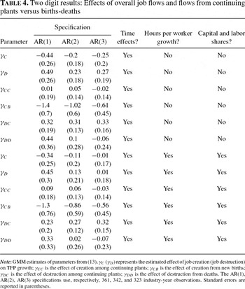
The results of two separate specifications, one that includes time effects and one in which I also add hours per worker growth and the capital and labor shares of total output, appear in Table 4. In an effort to be concise, I have only reported the GMM results. To begin, consider the estimated effects of overall creation and destruction, γC and γD. Although the majority of the estimates are insignificant, the signs and magnitudes of the coefficients are similar to what the four-digit data produced. Hence, at either level of aggregation, creation has an apparently negative effect on productivity growth, whereas destruction has a positive effect.

Looking at the separate influences of creation through continuing establishments as opposed to births, it is apparent that there is a difference between the two.30
Technically, Wald tests only reject the hypothesis that γCC and γCB are equal in two of the six instances.
For destruction, there also appears to be a difference between the effects of the two types of flows.31
Statistically, however, Wald tests do not reject the equality of γDD and γDC in any of the cases.
What do these findings suggest with regard to the vintage capital and job matching theories outlined in Section 2? According to the vintage capital view of job flows, one would expect the birth and death parameters, γCB and γDD, to be positive. Statistically, neither one is. On the contrary, γCB tends to be strongly negative. The implication from the job match-quality view is that the effect of creation among continuers, γCC, should be negative, but the effect of destruction among continuers, γDC, ought to be positive. Although there is little evidence of the former, there is relatively strong evidence of the latter. Thus, between these two theories, the job matching explanation is, again, more consistent with the findings, yet these data are not overwhelmingly supportive of either view.
CONCLUSION
Because job creation and destruction influence the cross-sectional distribution of productivity across existing employment relationships, job flows likely affect the rate at which aggregate productivity changes. This paper has offered evidence in support of this notion.
To recap, the findings indicate that, after accounting for the endogeneity of the job-flow series, TFP growth tends to be positively associated with job destruction, whereas negatively associated with job creation. This relationship holds at both the two- and four-digit levels but is particularly strong among four-digit industries. Between the two theoretical characterizations of employment variation surveyed, such evidence is more consistent with the job match-quality view than with the vintage capital (or pure creative-destruction) perspective.
A cursory look into the effects of different types of job flows offers some mixed results but a similar basic conclusion. Within two-digit manufacturing, job creation through plant births tends to be negatively associated with productivity growth, whereas destruction through deaths is only weakly associated with TFP growth. Neither result provides much evidence in favor of the vintage capital notion. Although the estimated impact of creation in continuing plants is weak, the effect of destruction in existing plants is quite strong. This latter finding, of course, is consistent with the job match-quality view.
Needless to say, these issues require a great deal more research. This paper has only taken a somewhat rudimentary look at the effect of job flows on productivity growth. Given the fundamentally micro-level nature of the theories discussed here, future work examining plant-level data (including data on individual workers at each establishment), rather than industry aggregates as employed here, would be of tremendous importance in gaining additional insight into these matters.
The views expressed herein are those of the author and do not represent the official positions of the Federal Reserve Bank of St. Louis or the Federal Reserve System.
APPENDIX