1. Introduction
China’s shadow banking experienced a boom after the 2008 financial crisis. As shown in Figure 1, the ratio of shadow banking loans to GDP increased from about 10% in 2008 to around 30% in 2013–2017. This dramatic and rapid rise has drawn significant interest both from academic researchers and policymakers. Some have paid close attention to the detailed structures of shadow banking activities and the quantity estimation (Ehlers, et al. Reference Ehlers, Kong and Zhu2018). Some have analyzed the driving forces behind the recent surge in shadow banking (Chen, et al. Reference Chen, Ren and Zha2018; Chen, et al. Reference Chen, He and Liu2020; Hachem and Song, Reference Hachem and Song2021). Some have focused on studying specific shadow banking activities and/or products (Allen, et al. Reference Allen, Qian, Tu and Yu2019; Acharya et al., Reference Acharya, Qian, Su and Yang2024; Allen et al., Reference Allen, Gu, Li, Qian and Qian2023). Additionally, some have presented the recent phenomenon from a historical perspective or through cross-country comparisons (Dang, et al. Reference Dang, Liu, Wang and Yao2019; Zhu, Reference Zhu2021; Allen and Gu, Reference Allen and Gu2021). However, few have directly focused on studying the welfare implications of China’s shadow banking activities from a macroeconomic perspective. This paper fills this gap by building a general equilibrium model that embodies key Chinese characteristics and quantifies the evaluation of shadow banking in the current context of China.
In order to accurately assess the role of shadow banking in China, several features are especially relevant. The first and perhaps the most fundamental feature is the prevalence of financial frictions. Many studies have analyzed the positive effect of financial intermediation on economic development. As extensively surveyed by Levine (Reference Levine and Levine2005), financial development indeed leads to economic growth. It is understandable that the financial sector is far less developed in China, due to the low capacity of financial intermediaries to efficiently channel funds, or partially due to the stringent government restrictions. Thus, it is reasonable and necessary to put the development of Chinese shadow banking in an environment with severe financial constraints. In particular, both Zhu (Reference Zhu2021) and Allen and Gu (Reference Allen and Gu2021) have argued that some shadow banking activities in China are efficiency-enhancing by overcoming these financial constraints. In line with this literature, as a starting point, we introduce a financial friction in terms of funding constraints of financial intermediation, following Gertler and Karadi (Reference Gertler and Karadi2011) and Gertler and Kiyotaki (Reference Gertler, Kiyotaki, Gertler and Kiyotaki2011, Reference Gertler and Kiyotaki2015). Our model thus potentially opens the door for shadow banking activities in China, as a developing country, to improve social welfare.
Growth of regular bank loans and shadow banking loans.

Second, the rise of shadow banking activities has been intensely involving in regulatory arbitrage. This is not surprising at all, since according to the Financial Stability Board, shadow banking by nature is “credit intermediation involving entities and activities outside the regulated banking system”. In the context of China, banking regulation is especially tight given the backgrounds of widespread government controls in the economy. These regulations take many different forms, including the conventional reserve and capital requirements, the unconventional liquidity regulations such as loan-to-deposit caps, and the even more specific and structural regulations that restrict and prohibit banks from lending to various industries or entities. Studies have argued that these regulations in China substantially generate unintended consequences by causing the expansion of shadow banking activities. In particular, Hachem and Song (Reference Hachem and Song2021) show that stricter liquidity regulations push banks to use off-balance-sheet saving instruments that are not subject to liquidity regulations, leading to a credit boom. Chen, et al. (Reference Chen, Ren and Zha2018) provide empirical evidence that contractionary monetary policy generates a rise in shadow banking loans, offsetting the expected decline of traditional bank loans and leading to an unexpected boom in the total credit. We follow this literature by building such a regulation arbitrage feature into the model to partially explain the emergence of shadow banking.
As noted, similar to the argument of Gertler, et al. (Reference Gertler, Kiyotaki, Prestipino, Gertler, Kiyotaki and Prestipino2016), the crucial point is the differentiation between regular banking and shadow banking. It could also be possible that shadow banking is driven by technological advances in intermediation, for instance, in terms of financial engineering such as those emerging in the US. However, both Dang, et al. (Reference Dang, Liu, Wang and Yao2019) and Allen and Gu (Reference Allen and Gu2021) point out that this is less the case in China, where financial engineering plays a minor role. To be more specific, as has been documented by Dang, et al. (Reference Dang, Wang and Yao2014) and Ehlers, et al. (Reference Ehlers, Kong and Zhu2018), the Chinese shadow banking is largely bank-centric, in the sense that banks are the key players of shadow credit intermediation. Banks cooperate with other financial institutions (e.g. trust companies, securities companies, and other financial management companies) and/or operate through the inter-bank markets to move the credit intermediation either off balance sheets, or hide it as non-loan assets on the balance sheet. Thus, through the shadow banking system, banks are able to evade the various regulations imposed on regular banking products. Given this consideration, as a modeling choice, we borrow the structure of financial intermediation of Gertler, et al. (Reference Gertler, Kiyotaki, Prestipino, Gertler, Kiyotaki and Prestipino2016) by placing the regular banks as a hub of funds. These banks raise funds from households and then can either issue regular loans by directly funding projects or channel them to shadow banks. On the other hand, enjoying the regulatory privilege, the shadow banks are not allowed to directly raise funds from households, except for the funds from regular banks.
Given the above discussions that regular banking in China faces financial frictions while the shadow banking helps to overcome such frictions, it is logical to predict that shadow banking shall be efficiency-enhancing. However, we argue that such a prediction is only a part of the whole picture. This leads us to the third feature of the Chinese financial sector, that is, the shadow banking activities in China are associated with more investment risk. It is well known that the Chinese government is especially conservative with respect to financial development. Some financial regulations are directly targeting risk containment, for example, by prohibiting lending to industries or entities that are regarded as “risky” (Zhu, Reference Zhu2021). Moreover, along this line, there is a prevalent phenomenon in the Chinese financial system, that is, the existence of implicit guarantees on returns of shadow banking products. Governments or the distributing banks are typically assumed to provide compensation to the suppliers of funds in case of default, although they have no such legal obligation to do so. Such a financial phenomenon in China has been intensively observed and discussed in the fields of policy and business and has also been formally documented and studied by research papers (Allen and Gu, Reference Allen and Gu2021). For example, Allen et al. (Reference Allen, Gu, Li, Qian and Qian2023) find that the yield spreads of trust products (an important type of shadow banking products) are lower when they are issued by trust companies controlled by state-owned enterprises, or sold by the five largest state-owned banks. They argue that this indicates that the implicit guarantees from the government or state-controlled financial intermediaries lead to a mispricing of risks in shadow banking products. Similar micro evidence from the wealth management products (WMPs) is also presented by Huang, et al. (Reference Huang, Huang and Shao2023). Therefore, in order to comprehensively evaluate the role of shadow banking in China, we explicitly model this dark side by introducing the endogenous choice of risk-taking by the shadow banks. Furthermore, such risk-taking behaviors rest on the existence of government implicit guarantees, that is, the implicit guarantee serves as an insurance compensation to encourage the strategic risk-taking decisions of shadow banks. We do not deny that financial institutions in China could literally provide the implicit guarantees. However, since the majority of the important financial institutions are owned and/or controlled by the governments at various levels, besides the public’s strong beliefs, it is reasonable to interpret that the governments are backing up these financial institutions and thus serve as the fundamental source of such guarantees in China.
Taking these features together, we demonstrate that the evaluation of shadow banking in China rests on three effects. The first effect is called the total capital effect. With the financial constraint on regular banks’ abilities to hold assets, there is an under-supply of capital, leading to a social welfare loss. The rise of shadow banks in the financial intermediary sector, induced either by regulation arbitrage or by insurance compensation in terms of implicit guarantees, improves social welfare by financing more capital production. The second effect is called the financing structure effect. Since the financing cost of shadow banking is higher, the substitution of regular loans with shadow banking products has negative impacts on social welfare by causing resource misallocations. Besides these two common effects, the implicit guarantees have a third effect, namely, the risk-taking effect, which encourages shadow banks to take excessive risks and deteriorates social welfare by wasting resources. We highlight that this risk-taking effect is very crucial in completely evaluating the role of shadow banking. We demonstrate that, without the channel of risk-taking, the expansion of shadow banking leads to an improvement in social welfare, since the total capital effect always dominates the financing structure effect.
With the calibrated model, we focus on the optimal degree of government guarantees to determine the optimal level of shadow banking in China as an illustration. We show that there exists an optimal insurance level that maximizes social welfare. Below this optimal level, providing more generous insurance to increase shadow banking boosts social welfare since the positive total capital effect dominates the negative financing structure effect and risk-taking effect. Beyond the optimal level, a further increase in shadow banking deteriorates social welfare in that the negative financing structure effect and the risk-taking effect dominate. Regarding the current situation of shadow banking in China, our quantitative results conclude that the level of shadow banking is excessively high. This implies that containing shadow banking activities by reducing regulation arbitrage allowance and/or implicit guarantees could improve social welfare. Thus, our quantitative conclusion indeed supports the recent policy movements of the Chinese government to regulate shadow banking.
Recently, there has been a growing literature on China’s shadow banking, and many of them are related to ours. Wang, et al. (Reference Wang, Wang, Wang and Zhou2015) find that shadow banking improves social surplus when the regular banking sector is distorted by a binding deposit rate ceiling and loan quota. While we agree with their evaluation of the positive side of shadow banking, we emphasize that the risk-taking side of shadow banking should not be neglected. Chang, et al. (Reference Chang, Liu, Spiegel and Zhang2019) study the optimal required reserve ratio in an environment that involves a trade-off between efficiency and risk: a higher required reserve ratio reallocates the resources from the state-owned sector to the more efficient private sector through shadow banking, but raises the default risks of the state-owned sector. By contrast, our work focuses on the welfare implications of shadow banking by directly modeling the risk-taking behaviors of financial intermediaries. Although several researchers, as mentioned, have raised concerns about the risks of implicit guarantees on shadow banking, few have studied them with general equilibrium models. Related to our paper, Dang, et al. (Reference Dang, Liu, Wang and Yao2019) build a theoretical model to show that the implicit guarantee is crucial in boosting shadow banking in China. However, unlike ours, they do not systematically study the welfare implications of shadow banking and the relevant optimal policies from a quantitative macroeconomic perspective.
Finally, our paper is certainly not the first one in the literature to have a focus on the dark side of shadow banking. As a matter of fact, there are emerging interests of research to study financial risk, especially after the 2008 financial crisis. However, mostly based on empirical phenomena in the US, more attention has been paid to particular financial stability issues such as rollover risk (Acharya, et al. Reference Acharya, Gale and Yorulmazer2011; Cheng and Milbradt, Reference Cheng and Milbradt2012; He and Xiong, Reference He and Xiong2012b), bank runs (Gertler, et al. Reference Gertler, Kiyotaki, Prestipino, Gertler, Kiyotaki and Prestipino2016) or debt runs (He and Xiong, Reference He and Xiong2012a). Some of the studies also introduce related financial stability frictions to evaluate policy options (Cheng and Milbradt, Reference Cheng and Milbradt2012; Huang, Reference Huang2018; Gertler, et al. Reference Gertler, Kiyotaki and Prestipino2020). Our paper complements them by focusing on the particular moral hazard problem of shadow banking, in terms of risk-taking behaviors induced by government implicit guarantees. We believe such a perspective is especially relevant and valuable for developing countries, for which some people may advocate that the governments should play more developmental roles in the financial sector. In addition, admittedly, the feature of implicit guarantees associated with shadow banking is not unique to China. For instance, Huang (Reference Huang2018) has specifically analyzed a situation that regular banks strategically extend implicit guarantees to shadow banks without a role of governments. We differ from it by emphasizing the governments as a source of implicit guarantees, in line with Dang, et al. (Reference Dang, Liu, Wang and Yao2019).
The rest of the paper is organized as follows. Section 2 presents the institutional background of China’s shadow banking. Section 3 presents the model, and Section 4 discusses the calibration of the model. In Section 5, we study the transition paths of key macroeconomic variables after two counterfactual policy changes. Section 6 examines the welfare implications of regulation arbitrage and implicit guarantees involved in shadow banking. Section 7 concludes the paper.
2. Institutional background
China’s shadow banking experienced a rapid expansion after the 2007–2008 financial crisis. As shown in Figure 1(A), the ratio o shadow banking loansFootnote 1 to GDP increased from about 10% in 2008 to around 30% in 2013–2017. Previous research on shadow banking (Dang, et al. Reference Dang, Wang and Yao2014; Acharya et al., Reference Acharya, Qian, Su and Yang2024; Hachem and Song, Reference Hachem and Song2021; Allen et al., Reference Allen, Gu, Li, Qian and Qian2023) attributes its fast growth to both structural and cyclical factors. Structurally, regulatory arbitrage plays an essential role in driving the growth of shadow banking. In China, banks’ lending through regular loans is subject to various price and quantity restrictions. The regulated lending rate is usually lower than the market-clearing level, so banks tend to ration credit to their preferred customers such as state-owned enterprises and large companies, which are believed to be safer. Meanwhile, the quantity of regular bank loans is constrained by regulatory or macroprudential policies such as requirements on loan-to-deposit ratios, capital ratios, and reserves. Compared to regular bank loans, shadow banking loans are exempt from many credit and macroprudential requirements, and their prices are closer to market-driven levels. On one hand, shadow banking loans meet the credit demand for those firms without access to regular bank loans. On the other hand, shadow banking helps banks extend credit creation beyond what is allowed by existing regulations.
The cyclical factors also contribute to the growth of the shadow banking. To cope with the 2007–2008 financial crisis, the Chinese government launched a large number of infrastructure projects to stimulate the economy, which boosted the demand for credit. However, the banks’ capacity for further expanding regular loans was soon limited by the loan-to-deposit ratio and minimum capital requirements. As a result, banks cooperated with other financial institutions to move the credit intermediation either off balance sheets, or hide it as non-loan assets on the balance sheet. Through these shadow banking activities, banks managed to circumvent the regulatory policies and further extended their lending capacities. As shown in Figure 1(B), both regular bank loans and shadow banking loans experienced a more than 30% growth in 2009. Nevertheless, the growth rate of regular loans dropped to below 20% in 2010, while the growth rate of shadow banking loans jumped to about 70% and remained greater than that of regular loans until 2014. Consequently, the ratio of shadow banking loans to the sum of shadow banking loans and regular bank loans increased from about 10% in 2008 to around 20% in 2014.
The forms and instruments of China’s shadow banking are diverse and constantly evolving. However, the fundamental purpose remains to engage in regulatory arbitrage, no matter how the structure of shadow banking changes. For instance, an early-stage form is called ”bank-trust cooperation.” Specifically, banks raise funds through issuing WMPsFootnote 2 and then channel the funds to trust companiesFootnote 3 that issue trust loans to firms. Since WMPs and the related investments in trust loans are recorded off-balance sheet, this bank-trust cooperation could expand credit without being constrained by the loan-to-deposit ratio and minimum capital requirements. In a more recent form, trust companies follow banks’ instructions to issue loans to banks’ customers, and in turn sell the beneficiary rights to the banks. Banks thereby become entitled to the full participation rights in the gains and losses of the trust loans. The beneficiary rights show up on the bank’s balance sheet as non-loan assets, which are subject to less stringent regulatory restrictions.
A large number of trust (entrusted) loans are channeled to risky borrowers such as real estate developers, local government financing platforms, and small and medium enterprises (Chen, et al. Reference Chen, Ren and Zha2018; Allen, et al. Reference Allen, Qian, Tu and Yu2019; Chen, et al. Reference Chen, He and Liu2020; Allen et al., Reference Allen, Gu, Li, Qian and Qian2023). However, most investors of WMPs care little about the risks involved in the underlying assets financed by the trust (entrusted) loans. Instead, investors pay more attention to the credibility and financial soundness of banks that issue WMPs because of the implicit guarantees perceived by investors (Acharya et al., Reference Acharya, Qian, Su and Yang2024; Allen et al., Reference Allen, Gu, Li, Qian and Qian2023). In fact, Allen et al. (Reference Allen, Gu, Li, Qian and Qian2023) find that 74% of default cases are fully compensated either by trust companies or local governments among the default trust products for which they can obtain loss coverage information between 2002 and 2018, which strengthens the investors’ belief in implicit guarantees.
The extraordinary growth of the shadow banking and the potential risks have prompted the government to tighten regulations. On the one hand, to curb regulatory arbitrage, the new regulations stipulate that trust (entrusted) loans disguised as non-loan assets on banks’ balance sheets should be given the same risk weight as regular loans when calculating the capital to risk-weighted assets ratio. On the other hand, the new regulations reiterate that banks cannot provide explicit or implicit guarantees to WMPs. As shown in Figure 1(B), the growth rate of shadow banking loans has been negative since 2018.
Structure of the model.

3. The model
We construct a general equilibrium model incorporating five distinct types of agents: households, goods producers, capital producers, regular banks, and shadow banks. Households supply labor, engage in consumption activities, and undertake saving behaviors. Goods producers hire labor and rent capital from both regular banks and shadow banks. Regular banks raise funds from households and allocate investments to regular loans, while also channeling funds to shadow banks. Capital producers procure inputs from goods producers, convert these inputs into capital-producing projects, and subsequently sell these projects to banks. In line with Gertler, et al. (Reference Gertler, Kiyotaki, Prestipino, Gertler, Kiyotaki and Prestipino2016), we posit that the ability of regular banks to raise funds is subject to constraints, and investing in shadow banks serves as a means for regular banks to alleviate these fund-raising constraints. Shadow banks in our model can be thought of as special purpose vehicles which manage the shadow banking products for regular banks. They make decisions regarding the capital structure and the project risk level. We rely on a moral hazard problem to model the risk-taking behavior of shadow banks, similar to Abbate and Thaler (Reference Abbate and Thaler2019). Shadow banks exploit the absence of commitment concerning project risks and strategically select risk levels. Ultimately, the liability funds invested in shadow banks may be partially compensated by guarantees provided by the government. Figure 2 illustrates the structure of the model.
In our model, one purpose of shadow banks is to help regular banks manage funds that are not subject to regulations. In reality, regular banks in China usually do not manage these funds by themselves. Instead, they channel funds to other financial intermediaries (e.g., trust companies and financial management companies) and direct these intermediaries to invest. Corresponding to the case that these financial management companies have some degrees of freedom in controlling the funds, we assume that shadow banks choose the risk of projects to maximize the profits earned by the equity funds provided by regular banks. By assuming that shadow banking products are managed by a separate vehicle, we specifically and explicitly model the risk-taking behaviors involved in shadow banking, unlike other papers in the literature (Chen, et al. Reference Chen, Ren and Zha2018; Hachem and Song, Reference Hachem and Song2021). Moreover, we are able to isolate the problem of choosing the risk of shadow banking from the other decisions, which increases the tractability of our model while maintaining a reasonable degree of realism.
3.1 Households
Households provide labor to goods producers, consume, and save. Following Gertler, et al. (Reference Gertler, Kiyotaki, Prestipino, Gertler, Kiyotaki and Prestipino2016), we assume that households provide project management services for regular banks and charge them a competitive price
 $f_{t\text{ }}$
per unit of project, where
 $f_{t\text{ }}$
is set to be equal to the marginal cost of providing the service. Households maximize the expected present value of lifetime utility as given by:
 \begin{equation} E_{0}\sum _{t=0}^{\infty }\beta ^{t}\left \{ \ln C_{t}-\eta \frac {L_{t}^{1+\phi }}{1+\phi }\right \} , \end{equation}
where
 $C_{t}$
is consumption and
 $L_{t}$
is labor supply. The parameter
 $\beta$
is the discount factor,
 $\eta$
denotes the relative importance of labor in utility, and
 $\phi$
denotes the inverse of the elasticity of labor supply.
In every period, households face the following constraints
 \begin{equation} C_{t}+D_{t}\leq W_{t}L_{t}+R_{t-1}D_{t-1}+\Pi _{t}+\Delta _{t}-\Upsilon _{t}, \end{equation}
where
 $D_{t}$
denotes deposits,
 $W_{t}$
stands for the wage rate,
 $R_{t}$
is the deposit rate,
 $\Pi _{t}$
denotes the dividends transferred from regular banks and capital producers,
 $\Delta _{t}$
is the profit obtained from project management services, and
 $\Upsilon _{t}$
represents a lump-sum tax. We assume that households are only able to deposit funds in regular banks since shadow banks do not have the capacity to directly raise funds from households.
3.2 Capital producers
The capital producers procure final goods as inputs, convert them into capital-producing projects and subsequently sell these projects to banks. There exist two distinct types of capital-producing technologies. The first is a risk-free method, through which one unit of project can deterministically generate one unit of capital. The second is a risky method, wherein one unit of project has a probability of
 $q_{t}$
of generating
 $\Theta _{t}(q_{t})$
units of capital and a probability of
 $1-q_{t}$
of yielding nothing. We assume that regular banks exclusively invest in risk-free projects, while shadow banks solely invest in risky projects.Footnote
4
Hence,
 \begin{equation} k_{r,t}^{i}=o_{r,t}^{i}; \end{equation}
and
 \begin{align} k_{s,t}^{\, j} &=o_{s,t}^{\, j}\Theta _{t}(q_{t}^{\, j})=o_{s,t}^{\, j}\left ( \omega _{1}-\frac {\omega _{2}}{2}q_{t}^{\, j}\right ) \text{ with probability of }q_{t}^{\, j}; \end{align}
 \begin{align} k_{s,t}^{\, j} &=0 \text{with a probability of }1-q_{t}^{\, j} \end{align}
where
 $o_{r,t}^{i}$
represents the size of risk-free project acquired by regular bank
 $i$
, and
 $o_{s,t}^{\, j}$
and
 $q_{t}^{\, j}$
, respectively, denote the size and risk level of risky project purchased by shadow bank
 $j$
;
 $k_{r,t}^{i}$
stands for the capital invested by regular banks, hereafter denoted as regular capital and
 $k_{s,t}^{\, j}$
represents the capital invested by shadow banks, hereafter denoted as shadow capital.
 $\Theta _{t}(q_{t})$
is inversely related to the success probability
 $q_{t}$
, indicating a higher return for taking greater risks.
At each period, capital producers purchase
 $I_{x,t}$
(
 $\{x\in r,s\}$
, where
 $r$
denotes the risk-free project and
 $s$
denotes the risky project) units of final goods and transform them into
 $O_{x,t}^{new}$
units of new project, incurring a capital adjustment cost
 $\Gamma$
,
 \begin{equation} O_{x,t}^{new}=(1-\Gamma (I_{x,t}/I_{x,t-1}))I_{x,t} \end{equation}
where
 $\Gamma (I_{x,t}/I_{x,t-1})=\kappa \lbrack (I_{x,t}/I_{x,t-1})-1]^{2}$
, the parameter
 $\kappa$
governs the magnitude of capital adjustment cost. Capital producers maximize their expected discounted profits as follows:
 \begin{equation} \max _{I_{x,t+i}}E_{t}\sum _{i=0}^{\infty }\beta ^{i}\frac {C_{t}}{C_{t+i}}\left [ Q_{x,t+i}(1-\Gamma (I_{x,t+i}/I_{x,t+i-1}))I_{x,t+i}-I_{x,t+i}\right ] \end{equation}
where
 $Q_{x,t}$
represents the price of projects. Additionally, at the beginning of each period, capital producers repurchase the existing projects after depreciation,
 $O_{x,t}^{old}=(1-\delta )K_{x,t-1}$
, from banks at the current market price
 $Q_{x,t}$
and then resell them in the market. Here
 $K_{r,t}$
and
 $K_{s,t}$
denote the aggregate amounts of
 $k_{r,t}^{i}$
and
 $k_{s,t}^{\, j}$
, respectively. Thus, the total quantity of projects available for sale in period
 $t$
is
 $O_{x,t}=$
 $O_{x,t}^{new}+$
 $O_{x,t}^{old}$
.
3.3 Regular banks
We assume that there is a continuum of regular banks indexed by
 $i\in \lbrack 0,1]$
. Each regular bank combines its own net worth,
 $n_{t}^{i}$
, and funds raised from households,
 $d_{t}^{i}$
, to make investments in both regular loans,
 $s_{t}^{i}$
, and shadow banking products,
 $b_{t}^{i}$
. The regular loans are utilized to acquire risk-free capital-producing projects,
 $o_{r,t}^{i}$
. We assume that regular banks purchase project management services from households at a price
 $f_{t}$
per unit of project, as in Gertler, et al. (Reference Gertler, Kiyotaki, Prestipino, Gertler, Kiyotaki and Prestipino2016). The budget constraint for regular banks is presented as follows:
 \begin{equation} s_{t}^{i}+b_{t}^{i}=[Q_{r,t}+f_{t}]o_{r,t}^{i}+b_{t}^{i}=n_{t}^{i}+d_{t}^{i}, \end{equation}
Following Gertler, et al. (Reference Gertler, Kiyotaki, Prestipino, Gertler, Kiyotaki and Prestipino2016), we assume that the capacity of regular banks to raise funds from households is constrained by minimum capital requirements. One interpretation of this financial friction is that regular bankers can divert assets for personal gain rather than operating with integrity. To incentivize regular banks’ investments in shadow banking products, we assume that diverting investments in shadow banking products is more difficult than diverting investments in regular loans. Specifically, we assume that depositors believe banks can divert
 $\theta$
percent of their regular loans, but only
 $\gamma$
percent of their investments in shadow banking products, where
 $\gamma \lt \theta$
. To rationalize this assumption, Gertler, et al. (Reference Gertler, Kiyotaki, Prestipino, Gertler, Kiyotaki and Prestipino2016) argue that interbank loans (an instrument for shadow banking) are less idiosyncratic in nature than non-financial loans and thus more amenable to monitoring by outside depositors. However, we interpret that banking regulatory authorities have their own evaluations of shadow banking products and can align depositors’ beliefs with their own. In this regard,
 $\gamma$
serves as a policy instrument: regulatory authorities can set the values of
 $\gamma$
to adjust the amount of regulatory arbitrage allowance enjoyed by shadow banks.
With the above assumptions, any financial agreement between regular banks and depositors should satisfy the following incentive constraint:
 \begin{equation} v_{t}^{i}\geq \theta (Q_{r,t}+f_{t})o_{r,t}^{i}+\gamma b_{t}^{i}, \end{equation}
which indicates that the franchise value of the bank,
 $v_{t}^{i}$
(to be defined later), should not be less than the gain from diverting funds. Given that the franchise value of a bank,
 $v_{t}^{i}$
, is positively correlated with its net worth,
 $n_{t}^{i}$
, Eq. (9) can be regarded as a minimum capital requirement for regular banks. This requirement stipulates that
 $\theta$
units of regular banks’ capital (net value) are needed for each unit of investment in regular loans and
 $\gamma$
units of regular banks’ capital are required for each unit of investment in shadow banking. When
 $\gamma \lt \theta$
, meaning that investments in shadow banking enjoy regulatory privilege, regular banks can alleviate the constraint imposed by the minimum capital requirement by reallocating investments from regular loans to shadow banking products. This assumption can also be reconciled with the fact that in China, some investments in shadow banking are recorded as interbank loans on commercial banks’ balance sheets and are considered less risky assets than regular loans when calculating the risk-based capital requirement.
According to Eq. (9), the limit on the total assets that a regular bank can hold is contingent upon its net value. If regular banks accumulate sufficient net value such that they no longer require external financing, the constraint ceases to be binding. To preclude this scenario, we assume that regular banks have a probability
 $\sigma$
of surviving until the next period and a probability of
 $1-\sigma$
of exiting the market. To maintain the total number of regular banks, new regular banks will enter each period with an initial endowment
 $w$
, financed by a lump-sum tax. As long as there is a positive probability that the regular banks’ capacity to raise funds may be constrained at some point in the future, it will be optimal for regular banks to defer dividends and accumulate net worth until exit. We assume that regular banks transfer net worth back to households and employ a stochastic discount factor
 $\Lambda _{t+m}=\beta ^{m}(C_{t}/C_{t+m})$
. Consequently, the expected utility of a continuing regular bank at the end of period
 $t$
is given by:
 \begin{equation} v_{t}^{i}=E_{t}\left [ \sum _{m=1}^{\infty }\Lambda _{t+m}(1-\sigma )\sigma ^{m-1}n_{t+m}^{i}\right ] , \end{equation}
where
 $(1-\sigma )\sigma ^{m-1}$
is the probability of exiting at date
 $t+m$
. Equation (10) can be rewritten as a recursive form:
 \begin{equation} v_{t}^{i}=E_{t}\left \{ \Lambda _{t+1}\left [ (1-\sigma )n_{t+1}^{i}+\sigma v_{t+1}^{i}\right ] \right \} =E_{t}\left [ \Omega _{t+1}^{i}n_{t+1}^{i}\right ] , \end{equation}
where
 $\Omega _{t+1}^{i}=\Lambda _{t+1}\left ( 1-\sigma +\sigma \frac {v_{t+1}^{i}}{n_{t+1}^{i}}\right )$
.
At each period, regular banks earn a return rate,
 $R_{k,t}^{r}$
on regular loans and a return rate,
 $R_{b,t}$
, on shadow banking investments. Thus, the net worth of a regular bank at period
 $t+1$
is:
 \begin{equation} n_{t+1}^{i}=R_{k,t+1}^{r}(Q_{r,t}+f_{t})o_{r,t}^{i}+R_{b,t+1}b_{t}^{i}-R_{t+1}d_{t}^{i}, \end{equation}
where
 $R_{k,t+1}^{r}=\frac {Q_{r,t+1}(1-\delta )+Z_{t+1}}{Q_{r,t}+f_{t}}$
. At period
 $t$
, each unit of regular loans can be utilized to acquire
 $1/(Q_{r,t}+f_{t})$
units of risk-free capital-producing projects. At period
 $t+1$
, each unit of capital yields a rental rate of capital
 $Z_{t+1}$
and a resale value
 $Q_{r,t+1}(1-\delta )$
, where
 $\delta$
represents the depreciation rate.
Therefore, the optimization problem for each regular bank is to choose
 $(o_{r,t}^{i},d_{t}^{i},b_{t}^{i})$
in order to maximize the bank value as given by Eq. (11), subject to the budget constraints Eqs. (8) and (12), as well as the incentive constraint specified in Eq. (9).Footnote
5
3.4 Shadow banks
There is a continuum of shadow banks, indexed by
 $j\in \lbrack 0,1]$
. They do not have the ability to directly obtain financing from households. Instead, they can acquire funds from regular banks either through liability funds or equity funds. Specifically, following Abbate and Thaler (Reference Abbate and Thaler2019), we assume that each shadow bank determines its capital structure by raising liability funds, denoted as
 $LF_{t}$
, and equity funds, denoted as
 $EF_{t}$
, from regular banks. The equity ratio of shadow banks is defined as
 $e_{t}^{\, j}=EF_{t}^{\, j}/(LF_{t}^{\, j}+EF_{t}^{\, j})$
. This assumption regarding the capital structure is made to facilitate the explanation of the inefficient risk-taking behavior of shadow banks. Based on this assumption, we further introduce a moral hazard problem associated with debts. We assume that the risk of capital-producing projects cannot be predetermined in the debt contract. Consequently, shadow banks always have an incentive to take on more risks. This is because they can reap all the benefits arising from higher risks while only partially bearing the associated costs. We will show that the implicit guarantees provided by the government have an impact on the optimal capital structure and, thus, affect the risk-taking behavior of shadow banks.
Each shadow bank is only permitted to invest in one risky capital-producing project with a size of
 $o_{s,t}^{\, j}$
at a unit price of
 $Q_{s,t}$
. They are confronted with investment risk: with a probability of
 $q_{t}^{\, j}$
, the project succeeds, and the shadow bank repays the liability funds at a promised return rate of
 $R_{l,t}$
and pays the equity funds a state-contingent return rate of
 $R_{e,t}$
. In the case where the probability is
 $1-q_{t}^{\, j}$
, the equity funds receive nothing, while the liability funds can still obtain some compensation from the government, which is financed by a lump-sum tax. We assume that this compensation amounts to
 $\Psi$
percent of the total assets managed by shadow banks,
 $LF_{t}^{\, j}+EF_{t}^{\, j}$
, indicating that each unit of liability funds can receive an amount of compensation equal to
 $\Psi /(1-e_{t}^{\, j})$
. Assuming that regular banks can fully diversify the idiosyncratic risks through investment in numerous different shadow banks, the no-arbitrage condition requires that:
 \begin{equation} E_{t}\left ( \Lambda _{t+1}R_{b,t}\right ) =E_{t}\left \{ \Lambda _{t+1}\left [ q_{t}^{\, j}R_{l,t}+(1-q_{t}^{\, j})\frac {\Psi }{1-e_{t}^{\, j}}\right ] \right \} =E_{t}\left ( \Lambda _{t+1}q_{t}^{\, j}R_{e,t+1}\right ) , \end{equation}
which implies that the expected payoffs, when discounted by the stochastic discount factor, ought to be identical. The compensation provided to liability funds functions as a subsidy for these liability funds. This, in turn, reduces the required rate of return for liability funds, thereby rendering equity funds relatively more expensive. We refer to
 $R_{b,t}$
as shadow banks’ financing cost thereafter because it determines regular banks’ expected rate of return when they channel funds to shadow banks.
Now, we introduce the moral hazard problem associated with risk-taking. We assume that shadow banks determine the risk level of projects by setting
 $q_{t}^{\, j}$
. However, this risk level cannot be prespecified in the debt contract with liability funds providers. In other words, even if shadow banks were to promise to take a certain risk level, they could easily renege on their promise and choose a different risk level to maximize the profits for equity holders. Shadow banks can do so because liability funds providers lack the ability to observe the actual project risk. Since both liability funds and equity funds are sourced from regular banks, to preserve the information friction, we assume that each regular bank has one department responsible for equity funds and another department responsible for liability funds, with the information sharing between these two departments prohibited. Anticipating this moral hazard problem, liability funds providers must first put themselves in the shoes of shadow banks and conjecture their optimal choice of risk level, and then accordingly determine the required return rate of debts,
 $R_{l,t}$
.
Specifically, with this timing structure, the optimization problem of shadow banks can be characterized as a two-stage problem. At the first stage, shadow banks choose the optimal capital structure,
 $e_{t}^{\, j}$
, while liability funds providers determine the required return rate of debts,
 $R_{l,t}$
, anticipating shadow banks’ risk choice. At the second stage, shadow banks select the optimal risk level,
 $q_{t}^{\, j}$
, given the capital structure
 $e_{t}^{\, j}$
and the return rate of debts,
 $R_{l,t}$
, specified in the first stage.
As a result, the optimization problem of shadow banks can be solved in a backward manner. At the second stage, given the required return rate of debts,
 $R_{l,t}$
, and the capital structure,
 $e_{t}$
, shadow banks select the project risk level,
 $q_{t}^{\, j}$
, in order to maximize the expected profits of equity funds providers:
 \begin{equation} \max _{q_{t}^{\, j}}Q_{s,t}o_{s,t}^{\, j}E_{t}\left \{ \Lambda _{t+1}\left [ q_{t}^{\, j}\left ( \omega _{1}-\frac {\omega _{2}}{2}q_{t}^{\, j}\right ) R_{k,t+1}^{s}-q_{t}^{\, j}R_{l,t}(1-e_{t}^{\, j})\right ] \right \} , \end{equation}
where
 $R_{k,t+1}^{s}=\frac {Z_{t+1}+(1-\delta )Q_{s,t+1}}{Q_{s,t}}$
is the rate of return on shadow capital. The first order condition with respect to
 $q_{t}^{\, j}$
is:
 \begin{equation} q_{t}^{\, j}=\frac {\omega _{1}E_{t}(\Lambda _{t+1}R_{k,t+1}^{s})-E_{t}(R_{l,t}\Lambda _{t+1})(1-e_{t}^{\, j})}{\omega _{2}E_{t}(\Lambda _{t+1}R_{k,t+1}^{s})}. \end{equation}
It is straightforward to demonstrate that
 $\frac {\partial q_{t}^{\, j}}{\partial e_{t}^{\, j}}\gt 0$
and
 $\frac {\partial q_{t}^{\, j}}{\partial R_{k,t+1}^{s}}\gt 0$
. This indicates that a higher leverage (lower
 $e_{t}^{\, j}$
) and a lower rate of return on shadow capital induce shadow banks to take greater risks (lower
 $q_{t}^{\, j}$
).
At the first stage, shadow banks determine the capital structure,
 $e_{t}^{\, j}$
, with the aim of maximizing the expected excess profits (profits net of the opportunity costs of equity), anticipating that
 $q_{t}^{\, j}$
will be selected at the second stage as a function of
 $e_{t}^{\, j}$
. Note that regular banks also anticipate the second-stage risk choice and price equity funds and liability funds accordingly. The shadow banks’ second-stage problem is therefore:
 \begin{equation} \max _{e_{t}^{\, j}}Q_{s,t}o_{s,t}^{\, j}E_{t}\left \{ \Lambda _{t+1}\left [ q_{t}^{\, j}\left ( \omega _{1}-\frac {\omega _{2}}{2}q_{t}^{\, j}\right ) R_{k,t+1}^{s}-q_{t}^{\, j}R_{l,t}(1-e_{t}^{\, j})-q_{t}^{\, j}R_{e,t+1}e_{t}^{\, j}\right ] \right \} , \end{equation}
subject to the constraints implied in Eq. (13),
 \begin{equation} E_{t}(\Lambda _{t+1}R_{l,t})=\frac {E_{t}\left [ \Lambda _{t+1}\left ( R_{b,t}-\frac {1-q_{t}^{\, j}}{1-e_{t}^{\, j}}\Psi \right ) \right ] }{q_{t}^{\, j}}\text{ and }E_{t}(\Lambda _{t+1}R_{e,t+1})=\frac {E_{t}\left ( \Lambda _{t+1}R_{b,t}\right ) }{q_{t}^{\, j}}. \end{equation}
We can substitute Eq. (17) into Eq. (16) and reformulate the shadow banks’ first stage problem as:
 \begin{equation} \max _{e_{t}^{\, j}}Q_{s,t}o_{s,t}^{\, j}E_{t}\left \{ \Lambda _{t+1}\left [ q_{t}^{\, j}\left ( \omega _{1}-\frac {\omega _{2}}{2}q_{t}^{\, j}\right ) R_{k,t+1}^{s}-R_{b,t}+(1-q_{t}^{\, j})\Psi \right ] \right \} . \end{equation}
The first order condition with respect to
 $e_{t}^{\, j}$
is given by
 \begin{equation} E_{t}\left [ \Lambda _{t+1}(\omega _{1}R_{k,t+1}^{s}-\omega _{2}q_{tt}^{\, j}R_{k,t+1}^{s}-\Psi )\right ] \frac {\partial q_{t}^{\, j}}{\partial e_{t}^{\, j}}=0. \end{equation}
Equation (19) demonstrates that shadow banks are faced with the following trade-off when determining the capital structure: increasing the equity ratio could incentivize shadow banks to choose projects with higher probability of success (higher
 $q_{t}^{\, j}$
); a higher probability of success leads to greater expected return from successful projects as long as
 $q_{t}^{\, j}\lt$
 $\omega _{1}/\omega _{2}$
, but results in less compensation from governments once projects fail. The presence of implicit guarantees from governments induces shadow banks to choose higher leverage (lower
 $e_{t}^{\, j}$
) even though they anticipate that a lower equity ratio leads to greater risk taking. Without the implicit guarantees from governments (
 $\Psi =0$
), the optimal condition regarding the choice of equity ratio Eq. (19) requires that
 $q_{t}^{\, j}=$
 $\omega _{1}/\omega _{2}$
, which can be achieved when shadow banks finance only through equity funds (
 $e_{t}^{\, j}=1$
, as shown by Eq. (15)).
Finally, the assumption of free entry into the shadow banking market ensures that the expected excess profit is zero:
 \begin{equation} E_{t}\left \{ \Lambda _{t+1}\left [ q_{t}^{\, j}\left ( \omega _{1}-\frac {\omega _{2}}{2}q_{t}^{\, j}\right ) R_{k,t+1}^{s}-R_{b,t}+(1-q_{t}^{\, j})\Psi \right ] \right \} =0. \end{equation}
Equation (20) indicates that a decline in the shadow banking financing cost
 $R_{b,t}$
or an increase in the level of government guarantees
 $\Psi$
attracts more funds to shadow banking, leading to an increase in the shadow capital and therefore a decrease in the rate of return on shadow capital
 $R_{k,t}^{s}$
.
We then combine Eq. (20) with Eqs. (15) and (19) to solve for the equity ratio
 $e_{t}^{\, j}$
and the project risk level
 $q_{t}^{\, j}$
:
 \begin{align} e_{t}^{\, j} &=\frac {\widetilde {R}_{b,t}-\widetilde {\Psi }}{\widetilde {R}_{b,t}}, \end{align}
 \begin{align} q_{t}^{\, j} &=1-\frac {\widetilde {R}_{b,t}}{\widetilde {\Psi }}+\frac {\sqrt {\omega _{2}(\widetilde {R}_{b,t}-\widetilde {\Psi })\left [ 2\omega _{1}\widetilde {\Psi }+\omega _{2}(\widetilde {R}_{b,t}-\widetilde {\Psi })\right ] }}{\omega _{2}\widetilde {\Psi }}, \end{align}
where
 $\widetilde {R}_{b,t}=E_{t}(\Lambda _{t+1}R_{b,t})$
and
 $\widetilde {\Psi }=E_{t}(\Lambda _{t+1}\Psi )$
.
With all the aforementioned results, we demonstrate that a higher ratio of government guarantees in the event of project failure reduces the required rate of return for liability funds,
 $R_{l,t}$
, making liability funds less costly than equity funds. This encourages the use of higher leverage, exacerbating the moral hazard problem and prompting shadow banks to take on greater risks. In addition, we show that both the equity ratio
 $e_{t}^{\, j}$
and the probability of success
 $q_{t}^{\, j}$
decrease as shadow banks’ financing cost
 $R_{b,t}$
declines. According to the zero-profit condition Eq. (20), a lower financing cost for shadow banks leads to more funds flowing to shadow banks and a decline in the rate of return on shadow capital,
 $R_{k,t}^{s}$
, thereby reducing the benefits of safer projects. This, in turn, induces shadow banks to choose riskier projects. Furthermore, as shown by the no-arbitrage condition Eq. (13), a decline in
 $R_{b,t}$
causes
 $R_{l,t}$
to decrease more than
 $R_{e,t}$
, making liability funds even less expensive relative to equity funds, which also induces a higher level of leverage.
3.5 Goods producers
Goods producers employ labor from households and rent capital from both regular banks and shadow banks. The production function is as follows:
 \begin{equation} Y_{t}=A_{t}L_{t}^{1-\alpha }K_{t-1}^{\alpha }. \end{equation}
where
 $K_{t}=K_{r,t}+K_{s,t}$
,
 $K_{r,t}$
represents the aggregate amount of regular capital and
 $K_{s,t}$
stands for the aggregate amount of shadow capital. We assume that regular capital and shadow capital are perfect substitutes in the process of goods production. Given the capital rental rate
 $Z_{t}$
and the wage rate
 $W_{t}$
, goods producers determine the demand for capital and labor so as to maximize their profits.
3.6 Aggregation and equilibrium
It is straightforward to show that
 $o_{r,t}^{i}/n_{t}^{i}$
,
 $d_{t}^{i}/n_{t}^{i}$
, and
 $b_{t}^{i}/n_{t}^{i}$
are identical for all regular banks provided that the marginal management cost of the risk-free project,
 $f_{t}$
, is independent of individual bank-specific factors. Here, in line with Gertler, et al. (Reference Gertler, Kiyotaki, Prestipino, Gertler, Kiyotaki and Prestipino2016), we assume that the marginal cost of project management service increases with the total project size, namely,
 $f_{t}=\varepsilon O_{r,t}$
(
 $\varepsilon \gt 0$
), where
 $O_{r,t}=\int _{0}^{1}o_{r,t}^{i}\,\text{d}i$
represents the total size of risk-free projects. Consequently, the total management cost is given by
 $F_{t}=\frac {1}{2}\varepsilon O_{r,t}^{2}$
. Under this condition, we can aggregate across banks in order to derive relations among the total net worth of all regular banks, denoted as
 $N_{t}=\int _{0}^{1}n_{t}^{i}\,\text{d}i$
, the sum of all household deposits,
 $D_{t}=\int _{0}^{1}d_{t}^{i}\,\text{d}i$
, the total investments in shadow banks,
 $B_{t}=\int _{0}^{1}b_{t}^{i}\,\text{d}i$
, and the total investments in risk-free projects
 $O_{r,t}$
:
 \begin{equation} (Q_{r,t}+f_{t})O_{r,t}^{{}}+B_{t}^{{}}=N_{t}^{{}}+D_{t}^{{}} \end{equation}
Meanwhile, the effective leverage
 $\Phi _{t}^{i}$
and the franchise value per unit of net worth
 $v_{t}^{i}/n_{t}^{i}$
are the same across all regular banks:
 \begin{align} \Phi _{t}^{i} &=\Phi _{t}=\frac {(Q_{r,t}+f_{t})O_{r,t}^{{}}+(\gamma /\theta )B_{t}^{{}}}{N_{t}^{{}}}, \end{align}
 \begin{align} \frac {v_{t}^{i}}{n_{t}^{i}} &=\frac {v_{t}}{n_{t}}=E_{t}\left \{ \Omega _{t+1}\left [ (R_{k,t+1}^{r}-R_{t+1})\Phi _{t}^{i}+R_{t+1}\right ] \right \} . \end{align}
The aggregate net worth of regular banks, denoted as
 $N_{t}$
, comprises two components. The first component is the accumulated net worth of banks that operated at time
 $t-1$
and survive until time
 $t$
. These surviving banks account for
 $\sigma$
percent of the total number of regular banks. Each of these surviving banks carries forward a net worth of
 $\left [ (R_{k,t}^{r}-R_{t})\Phi _{t-1}^{i}+R_{t}\right ] n_{t-1}^{i}$
. The second component is the endowment of entering banks, which account for
 $1-\sigma$
percent of total number of regular banks. Each entering bank brings forward an initial endowment of
 $w$
. Thus, the evolution of
 $N_{t}$
given by:
 \begin{equation} N_{t}=\sigma \left [ (R_{k,t}^{r}-R_{t})\Phi _{t-1}^{{}}+R_{t}\right ] N_{t-1}^{{}}+(1-\sigma )w \end{equation}
The aggregate capital supplied by regular banks is simply equal to the total size of all risk-free projects:
 $K_{r,t}=O_{r,t}.$
In equilibrium, all shadow banks choose the same capital structure and the same risk level, namely,
 $e_{t}^{\, j}=e_{t}$
and
 $q_{t}^{\, j}=q_{t}$
. Let
 $O_{s,t}=\int _{0}^{1}o_{s,t}^{\, j}dj$
denote the total size of risk projects. Then the aggregate shadow capital is given by
 $K_{s,t}^{{}}=\int _{0}^{1}o_{s,t}^{\, j}q_{t}^{\, j}\left ( \omega _{1}-\frac {\omega _{2}}{2}q_{t}^{\, j}\right )dj = O_{s,t}q_{t}^{{}}\left ( \omega _{1}-\frac {\omega _{2}}{2}q_{t}^{{}}\right ).$
Finally, the goods market clears when the output is equal to the sum of the consumption of households, the investments in risk-free and risky projects, and the management costs of regular bank projects:
 \begin{equation} Y_{t}=C_{t}+I_{r,t}+I_{s,t}+F_{t}. \end{equation}
The inter-bank funds market clears when the total demand for liability funds and equity funds by shadow banks is equal to the supply of funds from regular banks:
 \begin{equation*} \int _{0}^{1}(LF_{t}^{\, j}+EF_{t}^{\, j})dj=LF_{t}+EF_{t}=B_{t}. \end{equation*}
4. Calibration
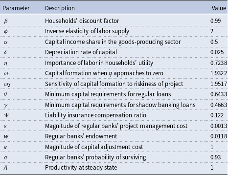
First, for some conventional parameters, we use standard values in the literature. In particular, we set the household’s subjective discount factor,
 $\beta$
, to
 $0.99$
. Following Chang, et al. (Reference Chang, Liu and Spiegel2015), the parameter
 $\phi$
is set to 2, which implies that the elasticity of labor supply is 0.5. We set
 $\alpha$
, the parameter that determines labor’s share of income in the goods-producing sector, to 0.5 as in Bai, et al. (Reference Bai, Hsieh and Qian2006) and Song, et al. (Reference Song, Storesletten and Zilibotti2011). The depreciation rate of capital,
 $\delta$
, is set to 0.025. The magnitude of the capital adjustment cost
 $\kappa$
is set to 1 as in Chang, et al. (Reference Chang, Liu, Spiegel and Zhang2019). The steady-state productivity level
 $A$
is normalized to 1.
Second, we calibrate the values of seven parameters (
 $\eta$
,
 $\omega _{1}$
,
 $\theta$
,
 $\varepsilon$
,
 $w$
,
 $\gamma$
,
 $\Psi$
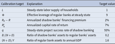
) jointly to hit seven targets at the steady state, which are summarized in Table 1. The labor supply
 $L$
is set to be 1. The leverage of regular banks
 $\Phi$
matches the average leverage ratios of commercial banks between 2009 and 2019, which are calculated based on the tier 1 bank capital. The shadow banks’ financing premium
 $R_{b}-R$
matches the average difference between the one year inter-bank offered rate and the one year deposit rate between 2009 and 2019. The rate of return of regular capital
 $R_{k}^{r}$
is set to match the estimated average capital return rates between 2009 and 2013 by Bai and Zhang (Reference Bai and Zhang2014).Footnote
6
Since small and medium size banks are more intensively involved in shadow banking business, we use the loan non-performing rate of small and medium banks to measure the project success rate of shadow banking
 $q$
. We collect the data on loan categorization of 274 banks in China from 2016 to 2019, and calculate the loan-size weighted average loan non-performing rate of those small and medium size banks.Footnote
7
The ratio of shadow banks’ assets to regular banks’ assets
 $B/(N+D)$
is set to match the average ratio of shadow banking loans (sum of trust loans, entrusted loans and bank acceptances) to the sum of regular loans and shadow banking loans between 2009 and 2019. The ratio of regular banks’ assets to annual GDP
 $(N+D)/Y$
targets the average ratio of the sum of regular loans and shadow banking loans to GDP between 2009 and 2019. In addition, we set
 $\omega _{2}=\omega _{1}/0.99$
so that the project-to-capital conversion rate of shadow banks,
 $t\equiv q_{t}^{{}}\left ( \omega _{1}-\frac {\omega _{2}}{2}q_{t}^{{}}\right )$
, is maximized at
 $q_{t}^{\ast }=0.99$
. In our model,
 $1-\sigma$
percent of regular banks exit and transfer their net value to households each period, and therefore
 $1-\sigma$
measures the aggregate regular banks’ dividends payout ratio. We set
 $\sigma$
to 0.93 to match the average dividends payout ratio for listed commercial banks in China between 2009 and 2019.
Calibration target

The values of all parameters are shown in Table 2. It is interesting to note that the calibrated value of
 $\Psi$
, the percentage of shadow banking losses covered by the government, is 0.122. It can be interpreted in two ways: first, on average 12.2% of losses suffered from defaulted shadow banking products will be covered by the government; second, there is a 12.2% chance that the government will bail out the project in trouble and fully compensate investors. The data on the loss coverage of shadow banking products is scarce. Allen et al. (Reference Allen, Gu, Li, Qian and Qian2023) collect the loss coverage information for 62 defaulted shadow banking products between 2002 and 2020 and find that about 19% of default cases (12 out of 62) are fully or partly compensated by the government.
Parameter values

5. Model simulations
In the model, there are two policy instruments: the regulatory arbitrage allowance of shadow banking, denoted by
 $\gamma$
, and the implicit government guarantees, represented by
 $\Psi$
. In this section, we conduct simulations of the model to examine their effects on the economy. We commence with an experiment in which we reduce
 $\gamma$
from its baseline value of 0.47 to 0.4, a change that can be regarded as a regulatory arbitrage shock. When
 $\gamma \lt \theta$
, investments through shadow banking enjoy regulatory privileges. Regular banks can relax the minimum capital requirements constraint by reallocating assets from regular loans to shadow banking loans. The lower
 $\gamma$
is, the stronger the incentive for regular banks to circumvent the minimum capital requirements. As illustrated in Figure 3, a decline in
 $\gamma$
reduces regular capital and increases shadow capital, which lowers the shadow banks’ financing cost,
 $R_{b,t}$
. According to Eqs. (21) and (22), a decline in financing costs further leads to a drop in the shadow banks’ equity-to-asset ratio (an increase in leverage) and a reduction in the probability of success of risky projects (an increase in risk level). Simultaneously, a decline in
 $\gamma$
and the increased flow of funds into shadow banking prompt regular banks to expand their total assets by attracting more deposits from households. It is the total assets of regular banks that determine the total capital amount. This explains why a decline in
 $\gamma$
leads to an increase in total capital, as shown in Figure 3. In the short run, households consume less; however, in the long run, the increase in output enables households to consume more. Moreover, the rise in total capital increases the marginal product of labor, leading to an increase in working hours.
The transition path of selected variables when
 $ \gamma$
declines.

The transition path of selected variables when
 $\Psi$
increases.

We next consider an experiment in which we increase the degree of implicit government guarantees, as measured by the liability insurance coverage ratio,
 $\Psi$
, from its baseline value of 12.2–14%. According to Eq. (13), this insurance functions as a subsidy for suppliers of liability funds. Consequently, an increase in
 $\Psi$
leads regular banks to reduce the interest rate,
 $R_{l,t}$
, charged on liability funds. This has two effects on shadow banks: firstly, they switch from equity financing to liability financing to capitalize on the relatively lower cost of liability funds compared to equity funds, as illustrated in Figure 4, which exacerbates the moral hazard problem by encouraging shadow banks to undertake greater risks in their projects. Secondly, as demonstrated by Eq. (16), a reduction in
 $R_{l,t}$
generates a positive excess profit, motivating shadow banks to increase their total financing from regular banks and invest in more projects. This accounts for the increase in capital financed by shadow banking, as depicted in Figure 4. In response to the surge in demand for funds from shadow banks, regular banks absorb more deposits from households and reduce their regular loans. The ability of regular banks to absorb more deposits stems from the easing of constraints imposed by the capital requirements, due to increased investments through shadow banking. The influx of deposits allows regular banks to hold more assets, so that the combined total of regular loans and shadow banking loans increases even as regular loans decrease. This explains the overall increase in the capital stock.
6. Welfare analysis
In the baseline model, there are two features associated with shadow banks. First, since regular banks face a constraint on their capacity to absorb deposits and expand asset holdings, shadow banks enjoy a regulatory privilege regarding capital requirements. Second, shadow banks can take advantage of the lack of commitment regarding their risk choices and thus take excessive risks. It would be interesting to examine how these features affect resource allocation and social welfare. Specifically, we analyze how two policy instruments, the degree of regulatory privilege,
 $\gamma$
, and the shadow banking liability insurance coverage ratio,
 $\Psi$
, could be adjusted to improve social welfare. Before conducting this analysis, we first explore an ideal situation in which a social planner can maximize households’ utilities by optimally allocating resources, overcoming all financial frictions and then use this as a criterion to assess the relative welfare losses in the decentralized economy.
6.1 The optimum with social planner
We assume that the social planner can optimally allocate resources without being concerned about the financial constraints. The planner maximizes social welfare by optimally choosing consumptions, hours worked, and investments in capital. There are two ways to produce capital: the first corresponds to the technique of regular banks, which involves management costs, while the second corresponds to the technique of shadow banks, which is characterized by a project-to-capital conversion rate of
 $t$
. We assume that the social planner always chooses the optimal risk level
 $q^{\ast }$
 $=0.99$
to maximize the expected project-to-capital conversion rate, and thus,
 $t^{\ast }=q_{{}}^{\ast }\left ( \omega _{1}-\frac {\omega _{2}}{2}q_{{}}^{\ast }\right ) =0.953$
. Additionally, to simplify the analysis, we ignore the capital adjustment cost.
Thus, the social planner chooses
 $C_{t}$
,
 $K_{t}$
,
 $K_{s,t}$
, and
 $L_{t}$
to maximize the household’s expected present value of lifetime utility:
 \begin{equation} E_{0}\sum _{t=0}^{\infty }\beta ^{t}\left \{ \ln C_{t}-\eta \frac {L_{t}^{1+\phi }}{1+\phi }\right \} , \end{equation}
subject to the following resource constraints:
 \begin{eqnarray*} C_{t}+I_{r,t}+I_{s,t}+F_{t} &\leq &A_{t}L_{t}^{1-\alpha }K_{t-1}^{\alpha }\text{,} \\ K_{r,t} &=&I_{r,t}+(1-\delta )K_{r,t-1}\text{,} \\ K_{s,t} &=&t^{\ast }\left [ I_{s,t}+(1-\delta )K_{s,t-1}\right ] \text{,} \\ K_{t} &=&K_{r,t}+K_{s,t}, \end{eqnarray*}
where
 $K_{r,t}$
and
 $K_{s,t}$
are capital produced using the techniques of regular banks and shadow banks, respectively.
 $F_{t}=\frac {1}{2}\varepsilon K_{r,t}^{2}$
is the management cost of producing regular capital.
The first order conditions with respect to
 $L_{t}$
,
 $K_{t}$
, and
 $K_{s,t}$
are as follows:
 \begin{align} (1-\alpha )A_{t}L_{t}^{-\alpha }K_{t-1}^{\alpha }/C_{t} &=\eta L_{t}^{\phi }, \end{align}
 \begin{align} 1+\varepsilon K_{r,t} &=\beta E_{t}\left \{ \frac {C_{t}}{C_{t+1}}\left [ \alpha A_{t+1}L_{t+1}^{1-\alpha }K_{t}^{\alpha -1}+1-\delta \right ] \right \} , \end{align}
 \begin{align} 1/t^{\ast } &=1+\varepsilon K_{r,t}. \end{align}
Equation (30) is the optimality condition for labor. Equation (31) describes the optimality conditions for the total capital, equating the marginal benefit and cost of acquiring an additional unit of capital. Equation (32) indicates that the marginal cost of producing additional regular capital and shadow capital should be the same. Note that the marginal cost of producing regular capital depends on the project management cost, while the marginal cost of producing shadow capital depends on the project-to-capital conversion rate
 $t$
.
6.2 Obtaining the first best in decentralized economy
We now examine whether the first-best equilibrium can be achieved in the decentralized economy. Specifically, the first-best equilibrium necessarily requires that Eqs. (30)–(32) are satisfied. Since there are no frictions in the labor market, Eq. (30) can always be achieved in the decentralized economy. Thus, we focus on the two optimality conditions governing capital accumulation, namely, Eqs. (31) and (32). The optimality condition Eq. (31) requires that the total capital reach a level such that the marginal benefit of investing an additional unit of capital equals the marginal cost. The optimality condition Eq. (32) requires that resources are appropriately allocated to regular banks and shadow banks so that the marginal cost of acquiring an additional unit of capital is equal regardless of whether it is financed by regular banks or shadow banks. In the online Appendix C, we prove that Eqs. (31) and (32) can only be achieved when the constraint on regular banks’ capacity for asset holding is slack and the shadow banking insurance coverage ratio is zero. In other words, as long as the constraint on regular banks’ capacity for asset holding is binding, it is impossible to satisfy the two optimality conditions simultaneously in the decentralized economy. This is because the capital requirements impose a constraint on regular banks’ capacity to absorb deposits and thus prevents the total capital from reaching the optimal level required by Eq. (31).
To further illustrate the role of the capital requirements, we consider a special case of the baseline model with no regulatory arbitrage (
 $\gamma$
equals
 $\theta$
) and no implicit government guarantees (
 $\Psi$
equals zero). In this special case, according to Eqs. (21) and (15), shadow banks will only use equity funds and choose the optimal level of risk,
 $q=q^{\ast }=0.99$
. Under this circumstance, the only friction preventing us from reaching the first-best resource allocation is the constraint imposed on the regular banks’ capacity to absorb deposits and expand asset holdings, measured by
 $\theta$
. Figure 5 shows how the key variables depend upon
 $\theta$
in the steady state. First of all, as shown by the figure, when
 $\theta$
approaches to zero, the constraint limiting the regular bank’s capacity to absorb deposits and expand asset holdings is relaxed. All the key variables and household utility converges to the first-best level. Meanwhile, as shown in Figure 5(f), both the rate of return on regular capital
 $R_{k}^{r}$
and the rate of return on shadow banking investments
 $R_{b}$
approach to the deposit rate
 $R$
(
 $R=1/\beta =1.01$
),Footnote
8
which is a criterion of obtaining the first best. As
 $\theta$
increases, the constraint on regular banks’ capacity to absorb deposits and expand asset holdings is tightened, causing a decline in the total capital (Figure 5(d)) and an increase in the rate of return
 $R_{k}^{r}$
and
 $R_{b}$
(Figure 5(f)), leading to a drop of the household’s utility (Figure 5(a)).
Particularly, we can identify a critical value
 $\theta ^{\ast }$
denoted by triangles in Figure 5. When
 $\theta \geq \theta ^{\ast }$
, the marginal cost of producing regular capital is lower than that of shadow capital (Figure 5(e)). Consequently, all capital will be intermediated by regular banks. As
 $\theta$
decreases, the increasing amount of regular capital drives up the management cost, eroding the regular banks’ cost advantage. When
 $\theta \lt$
 $\theta ^{\ast }$
, the most cost-effective approach is to maintain regular capital at
 $K_{r}(\theta ^{\ast })$
and let shadow banks finance the remainder, so that the marginal costs of producing regular capital and shadow capital are equal.
The impact of
 $ \theta$
on key variables and social welfare.

6.3 Finding the second best
Taking as given the constraint on regular banks’ capacity to absorb deposits and expand asset holdings, we are left with two policy instruments to utilize. The first policy instrument pertains to the degree of regulatory arbitrage allowance, governed by
 $\gamma$
, and the second instrument pertains to the percentage of shadow banking losses covered by government implicit guarantees, governed by
 $\Psi$
. In the following experiments, we focus on identifying the second best in the decentralized economy by varying these policy instruments, considering that the regular banks’ capacity to absorb deposits and expand asset holdings is always constrained by their net worth. We commence by examining the impact of
 $\gamma$
on resource allocations and welfare, holding
 $\Psi$
constant, and then proceed to explore the impact of
 $\Psi$
, holding
 $\gamma$
constant. In this manner, we investigate under the assumption that different governmental authorities make decisions independently, taking the choices made by others as given. For instance, in the context of China, we could interpret this as the banking regulatory authority governs
 $\gamma$
, while local governments determine the value of
 $\Psi$
. The coordination of these two policy instruments will be studied in the next section.
6.3.1 The impact of
 $ \gamma$
given
$\Psi$


We first explore the impact of the degree of regulatory arbitrage allowance,
 $\gamma$
, on resource allocation and social welfare. In doing so, we assume that the value of
 $\gamma$
is less than
 $\theta$
so that investments in shadow banking enjoy regulatory privilege. Figure 6 shows how the key variables depend on
 $\gamma$
in the steady state. A drop in
 $\gamma$
means that investments in shadow banking can relax the constraint on regular banks’ capacity for asset holdings, thereby boosting the incentive to supply funds to shadow banks.
The solid lines in Figure 6 represent the scenario where there are no government guarantees, i.e.,
 $\Psi =0$
. As shown in Figure 6(f), a decrease in
 $\gamma$
reduces the required rate of return on shadow banking investments for regular banks,
 $R_{b}$
, and consequently lowers the financing cost of shadow banks. However, there exists a critical level of
 $\gamma ^{\ast \text{ }}=0.39$
(triangles in Figure 6(b)); beyond this point, the profit of shadow banks becomes negative, and thus no capital will be intermediated by shadow banks. Only when
 $\gamma \lt$
 $\gamma ^{\ast \text{ }}$
and the financing cost of shadow banks drops to a sufficiently low level can shadow banks break even and begin to finance shadow capital. As
 $\gamma$
continues to decline, more capital is intermediated by shadow banks, partially substituting for the capital originally financed by regular banks. Meanwhile, regular banks attract more deposits and expand their total assets, resulting in an increase in the total capital.
The impact of
 $ \gamma$
on key variables and social welfare.

The household’s steady-state utility continuously increases as
 $\gamma$
declines, attaining its highest level when
 $\gamma$
approaches zero. However, even at this peak level, the household’s steady-state utility remains 0.4% lower than the first-best level. To understand how the household’s utility changes with respect to
 $\gamma$
, we derive the total derivative of the steady-state utility
 $U$
with respect to
 $\gamma$
as follows (see online Appendix D for details):
 \begin{equation} \frac {dU}{d\gamma }=\frac {1}{C}\left \{ \Omega _{K}\frac {\partial K}{\partial \gamma }-\Omega _{K_{s}}\frac {\partial K_{s}}{\partial \gamma }+\Omega _{q}\frac {\partial q}{\partial \gamma }\right \} \end{equation}
where
 $\Omega _{K}=(Z+1-\delta )-(1+\varepsilon K_{r})$
,
 $\Omega _{K_{s}}=1/t-(1+\varepsilon K_{r})$
, and
 $\Omega _{q}=\frac {K_{s}}{t^{2}}\left ( \omega _{1}-\omega _{2}q\right )$
. The term
 $\Omega _{K}$
represents the marginal net benefit of an additional unit of total capital when financed by regular banks.
 $\Omega _{K}$
is positive provided that
 $R_{k}^{r}=\frac {Z+1-\delta }{1+\varepsilon K_{r}}\gt 1$
. The term
 $\Omega _{K_{s}}$
represents the marginal extra cost of financing through shadow banks. This cost is positive when the marginal cost of shadow capital
 $1/t$
exceeds that of regular capital
 $1+\varepsilon K_{r}$
. Meanwhile,
 $\Omega _{q}$
represents the marginal benefit of reducing the shadow banks’ project risk level, and it is always positive. Consequently, we can decompose the impact of
 $\gamma$
on the steady-state household utility
 $U$
into three components. The first component,
 $\Omega _{K}\frac {\partial K}{\partial \gamma }$
, is termed the total capital effect. The second component,
 $\left ( -\Omega _{K_{s}}\frac {\partial K_{s}}{\partial \gamma }\right )$
, is labeled the financing structure effect. And the third component,
 $\Omega _{q}\frac {\partial q}{\partial \gamma }$
, is referred to as the risk-taking effect. As shown in Figure 6(d), an increase in
 $\gamma$
leads to a decline in the total capital, and thus the total capital effect of a rising
 $\gamma$
is negative. Figure 6(b) shows that an increase in
 $\gamma$
results in a decrease in the capital intermediated by shadow banks, and so
 $\frac {\partial K_{s}}{\partial \gamma }\lt 0$
. This means that the financing structure effect of a rising
 $\gamma$
is positive. As shown in Figure 6(g), changes in
 $\gamma$
cause negligible variations in the shadow bank project risk, and consequently, the risk-taking effect is close to zero. Overall, in Figure 6(h), we demonstrate that the marginal utility gain
 $\frac {dU}{d\gamma }$
is negative for
 $\gamma \lt \gamma ^{\ast }$
. On one hand, a decline in
 $\gamma$
increases the total capital amount by relaxing the constraint on regular banks’ capacity for asset holdings, which improves social welfare. On the other hand, as
 $\gamma$
declines, more capital is financed through the more costly shadow banking, having a negative impact on social welfare. When the total capital effect outweighs the financing structure effect, social welfare improves as
 $\gamma$
decreases. This explains why a decline in
 $\gamma$
(for
 $\gamma \lt \gamma ^{\ast }$
) leads to an increase in the household’s steady-state utility level.
We then examine scenarios where the government covers part of the losses of shadow banking products. The dashed lines in Figure 6 illustrate the resource allocation and welfare changes for various values of
 $\gamma$
when
 $\Psi$
is set to the calibrated value of 0.122, while the dash-dotted lines represent the situation where
 $\Psi$
is set to 0.14. Government compensation leads to an increase in shadow capital, a decrease in regular capital, and an increase in total capital for any level of
 $\gamma$
. Meanwhile, it prompts shadow banks to take on more risks, thereby reducing the project-to-capital conversion rate and resulting in a higher extra cost of shadow capital,
 $\Omega _{K_{s}}$
. Regarding the welfare implications, as shown by the dashed line in Figure 6(a), the utility reaches its maximum at
 $\gamma =0.5$
when
 $\Psi = 0.122$
. However, for
 $\Psi = 0.14$
, the utility gain from the financing structure effect consistently outweighs the utility loss due to the total capital effect as
 $\gamma$
increases. The dash-dotted line in Figure 6(a) indicates that the utility is maximized only when
 $\gamma$
equals
 $\theta$
, at which point regulatory arbitrage disappears. Overall, these experimental results suggest that the presence of government compensation modifies the trade-off between the total capital effect and the financing structure effect.
6.3.2 The impact of
$\Psi$
given
$ \gamma$


Next, we analyze the impact of implicit government guarantees, denoted as
 $\Psi$
, on social welfare, while holding the value of
 $\gamma$
constant. The government guarantees serve as insurance for liability funds invested in shadow banking projects, facilitating the shadow banks’ ability to break even.
The impact of
 $\Psi$
on key variables and social welfare.

The solid lines in Figure 7 illustrate how the key variables vary with
 $\Psi$
in the steady state when
 $\gamma$
is set to the baseline value of 0.4663. As depicted in Figure 7(b), when the insurance coverage ratio exceeds a critical value
 $\Psi ^{\ast }$
(marked with triangles in Figure 7), shadow banking projects start to generate non-negative profits, thereby enabling financing through shadow banks. As
 $\Psi$
continues to rise, not only does a larger proportion of the total capital get financed by shadow banks, but also the total capital also increases. More significantly, an increase in
 $\Psi$
leads to a substantial decline in the success probability of shadow banking projects (Figure 7(g)), which rapidly drives up the marginal cost of shadow capital (Figure 7(e)).
Regarding welfare, the solid line in Figure 7(a) shows that the utility attains its maximum level at
 $\Psi ^{\ast \ast }=0.105$
, which remains 0.8% lower than the first-best level. To understand this phenomenon, we derive the total derivative of the steady-state utility
 $U$
with respect to
 $\Psi$
(the derivation is similar to that of
 $\frac {dU}{d\gamma }$
):
 \begin{equation} \frac {dU}{d\Psi }=\frac {1}{C}\left \{ \Omega _{K}\frac {\partial K}{\partial \Psi }-\Omega _{K_{s}}\frac {\partial K_{s}}{\partial \Psi }+\Omega _{q}\frac {\partial q}{\partial \Psi }\right \} \end{equation}
where the definitions of
 $\Omega _{K}$
,
 $\Omega _{K_{s}}$
, and
 $\Omega _{q}$
are the same as in Eq. (33). The impact of
 $\Psi$
on the steady-state utility is decomposed into three parts once again: the total capital effect,
 $\Omega _{K}\frac {\partial K}{\partial \Psi }$
; the financing structure effect,
 $\left ( -\Omega _{K_{s}}\frac {\partial K_{s}}{\partial \Psi }\right )$
; and the risk-taking effect,
 $\Omega _{q}\frac {\partial q}{\partial \Psi }$
. First,
 $\Omega _{K}$
is positive and when
 $\Psi \gt \Psi ^{\ast }$
, an increase in
 $\Psi$
results in an increase in the total capital. Consequently, the total capital effect of a rising
 $\Psi$
is positive. Second, as shown in Figure 7(e), the marginal extra cost of shadow capital,
 $\Omega _{K_{s}}$
, is positive. Meanwhile, Figure 7(e) also shows that an increase in
 $\Psi$
leads to a rise in the capital intermediated by shadow banks. As a result, the financing structure effect of a rising
 $\Psi$
is negative. Third,
 $\Omega _{q}$
is always positive. As indicated by Figure 7(g), an increase in
 $\Psi$
reduces the success probability of shadow banking projects. Thus, the risk-taking effect is negative. The optimal policy choice of the insurance coverage ratio,
 $\Psi$
, hinges on the trade-off among the three aforementioned effects. With regard to the total capital effect, an increase in
 $\Psi$
offers greater incentives to finance capital through shadow banking. This, in turn, drives the total capital closer to the socially optimal level, thereby enhancing social welfare. However, an increase in
 $\Psi$
also exerts negative impacts on social welfare via the risk-taking effect and the financing structure effect. As
 $\Psi$
rises, shadow banks exploit the lack of commitment regarding their risk choices and thus take on excessive risks. Consequently, the capital intermediated by shadow banks becomes even more costly.
For the baseline value of
 $\gamma =0.4663$
, Figure 7(a) indicates that social welfare reaches its maximum at
 $\Psi ^{\ast \ast }=0.105$
. This can be explained by referring to Figure 6(h). The marginal utility gain,
 $\frac {dU}{d\Psi }$
, is positive when
 $\Psi \lt \Psi ^{\ast \ast }$
, implying that the total capital effect dominates the financing structure effect and the risk-taking effect. Conversely, when
 $\Psi \gt \Psi ^{\ast \ast }$
, the marginal utility gain,
 $\frac {dU}{d\Psi }$
, becomes negative, implying that the financing structure effect and the risk-taking effect assume greater significance than the total capital effect. Notably and intriguingly, the value of
 $\Psi =0.122$
in the baseline model surpasses this optimal level. Although a higher
 $\Psi$
yields a total capital amount closer to the first-best level, this advantage cannot compensate for the cost associated with the greater risk-taking of shadow banks and the higher marginal cost of capital intermediated by them. Reducing the degree of implicit guarantees,
 $\Psi$
, from 0.122 to the optimal level would decrease the ratio of shadow capital to regular capital from 24.2% to 15.5%, resulting in a 0.1% improvement in welfare.
Finally, we conduct experiments to demonstrate that the optimal choices of
 $\Psi$
are dependent on the value of
 $\gamma$
. As indicated by the dashed line in Figure 6(a), when
 $\gamma =0$
, the utility reaches its maximum only when the government compensation rate is zero. In this scenario (
 $\gamma =0$
), with regular banks already having a strong incentive to channel funds to shadow banking investments through regulatory arbitrage, total capital is not scarce. The adverse effect of inducing shadow banks to take more risks due to government guarantees dominates, and thus any provision of such insurance would worsen social welfare. In another extreme case, when we eliminate the possibility of regulatory arbitrage by setting
 $\gamma =\theta$
, as shown by the dash-dotted lines in Figure 6, regular banks only have sufficient incentive to invest in shadow banking projects when the government provides a higher loss guarantee compared to the baseline case.
6.4 Coordination of two policy instruments
The above experiments imply that the optimal choices of
 $\gamma$
and
 $\Psi$
are interdependent. In this section, we further investigate the coordination between these two policy instruments by presenting all possible outcomes across different levels of
 $\gamma$
and
 $\Psi$
. Figure 8 presents these results regarding social welfare and total capital. Specifically, in the upper panel of Figure 8, we graph the utility values as elevations above a grid in the
 $\gamma -\Psi$
plane; whereas in the middle and lower panels, we depict the levels of utility and total capital under various combinations of
 $\gamma$
and
 $\Psi$
using distinct colors, with warmer hues indicating higher levels.
The plots in Figure 8 show that the maximum welfare level can be obtained when shadow banks have the largest amount of regulatory arbitrage (
 $\gamma =0$
) and simultaneously, the government provides no guarantees for shadow banking products (
 $\Psi =0$
). However, it is realistic to suspect whether this cooperative outcome could be achieved in the context of China. For instance, if, as interpreted, the banking regulation authority sets the capital requirement, and on the other hand, local governments provide guarantees for shadow banking finance, it is legitimate to expect that local governments have strong incentives to stimulate capital investment, which is a key engine for economic growth. In this case, as shown by the lower panel of Figure 8, local governments always have incentives to increase
 $\Psi$
given any value of
 $\gamma$
, since doing so can expand total capital. With local governments’ distorted incentives, in order to maximize social welfare, the optimal response of the banking regulation authority is to adjust the level of regulatory arbitrage allowance by setting
 $\gamma$
. This non-cooperative equilibrium leads to a lower welfare level than the cooperative equilibrium. For instance, when the level of government guarantees is capped at 15% due to a fiscal constraint, the non-cooperative equilibrium (northeast corner in the middle panel of Figure 8) generates a level of welfare 0.83% lower than that at the cooperative equilibrium.
Welfare and total capital under various combination of
 $ \gamma$
and
 $\Psi$
.

6.5 The optimal policies under different
$ \theta$

In the model, the parameter
 $\theta$
measures the constraint that limits the capacity of regular banks to absorb deposits and expand asset holdings. In reality, the level of this constraint depends on the development of the financial sector and government intervention. Thus, it is reasonable to assume that different countries and/or economies have different values of
 $\theta$
. In order to generalize some implications for cross-country comparisons and investigate the sensitivity of optimal policies to
 $\theta$
, in this section, we conduct experiments to explore the impacts of the parameter
 $\theta$
.
In Figure 9, we plot resource allocations and corresponding welfare levels for a country with a relatively lower bank capital requirement (
 $\theta =0.5$
) and a country with a relatively higher bank capital requirement (
 $\theta =0.8$
), along with the baseline case. As shown in the figure, a higher bank capital requirement for regular loans provides banks with greater incentives to channel funds through shadow banking (Figure 9-b) and results in a lower required return for shadow banking investments (Figure 9-b). Specifically, the lower financing cost makes it easier for shadow banks to break even. Consequently, shadow banking emerges in countries with higher capital requirements for regular loans, even when the government provides no guarantees for losses (
 $\Psi =0$
) from shadow banking investments, as indicated by the solid line in Figure 9(b).
Regarding the roles of government guarantees, the figure illustrates that they can narrow the capital gap (Figure 9-d) and the welfare gap (Figure 9-a) between countries with a high level of constraint and those with a low level of constraint. It is interesting to note that the total capital in a country with a higher banking capital requirement can exceed that in a country with a lower requirement when the level of government guarantees exceeds a threshold, as shown in Figure 9(d). However, even in this case, its social welfare remains lower, as shown in Figure 9(a), because more capital is financed through costly and risky shadow banking. Moreover, we also demonstrate that countries facing more constraints can benefit more from government guarantees. In particular, compared with the case without any support, government guarantees can enhance welfare by up to 0.34% in a country with a higher banking capital requirement (
 $\theta =0.8$
), whereas they only increase welfare by up to 0.26% in a country with a lower banking capital requirement (
 $\theta =0.5$
). This is because, in countries with fewer constraints, regular banks have an incentive to invest in shadow banking projects only when governments provide sufficiently high loss guarantees. Consequently, the welfare gain from shadow banking is limited as the guarantees encourage excessive risk-taking and their negative effects quickly predominate.
The optimal policies under various values of
 $ \theta$
.

The dynamics of welfare during the transition path.

6.6 Dynamic welfare analysis
We have examined the welfare changes at the steady states in the previous experiments. In this section, we further investigate the welfare dynamics associated with policy changes along the entire transition path between the initial steady state and the terminal state.Footnote
9
Figure 10 plots the transition paths of household utility, consumption, hours worked, and total capital when the degree of implicit government guarantees,
 $\Psi$
, is reduced from 0.122 to 0.105 and other parameters are held constant at their baseline values. The vertical axis reports the percentage deviations from the initial steady state, and the horizontal axis shows the time elapsed. As shown in Figure 10, a reduction in implicit guarantees leads to a decline in the capital stock, making more resources available for consumption during the first 100 periods after the policy change. Meanwhile, households work fewer hours and thus enjoy a higher utility. At the peak level, households can enjoy a utility that is 0.38% higher than that in the initial steady state. Nevertheless, households still achieve a gain of about 0.1% in utility at the terminal steady state, even though the consumption level decreases by 0.3%, because the benefit of having more leisure outweighs the cost of reduced consumption. Overall, the results in Figure 10 indicate that households experience an increase in utility throughout the entire transition path following the policy change.
It would be interesting to further quantify the long run benefit of the above policy change by comparing the welfare effect of transition and the welfare effect of staying at the initial steady state. Specifically, we measure the effect of transition by calculating the weighted sum of households’ instantaneous utility over 5000 periods after the policy change:
 \begin{equation*} \text{Wel}_{trans}=\sum _{j=0}^{5000}\beta ^{\, j}\left \{ \ln C_{j}-\eta \frac {L_{j}^{1+\phi }}{1+\phi }\right \} , \end{equation*}
where
 $\left \{ C_{j},L_{j}\right \} _{j=0}^{5000}$
denotes the transition path of variables, and we measure the welfare effect of maintaining status quo as:
 \begin{equation*} \text{Wel}_{ss}=\sum _{j=0}^{5000}\beta ^{\, j}\left \{ \ln C_{0}-\eta \frac {L_{0}^{1+\phi }}{1+\phi }\right \} , \end{equation*}
where
 $C_{0}$
and
 $L_{0\text{ }}$
denote the initial steady state. We find that
 $\text{Wel}_{trans}$
is 0.12% higher than
 $\text{Wel}_{ss}$
, indicating that the policy change of lowering implicit government guarantees from the current level 0.122 to the optimal level 0.105 suggested by our study could benefit the economy in the long run.
7. Conclusion
An essential feature of China’s shadow banking is the prevalence of implicit guarantees on shadow banking products ultimately backed by the government. Although previous researchers have raised concerns about the risks of implicit guarantees on shadow banking, few have studied its welfare implications. This paper examines this problem by constructing a model in which shadow banking is driven by regulatory arbitrage and implicit guarantees. Compared with regular loans, shadow banking loans are subject to fewer regulations, which prompts banks to circumvent the regulations by shifting regular loans to shadow banking loans. Meanwhile, investments in shadow banking could be partially compensated by government guarantees in case of a project failure, which spurs the strategic risk-taking behavior of shadow banks.
We find that shadow banking has the potential to enhance social welfare by alleviating constraints on banks’ ability to expand credit. However, it may also have adverse effects on social welfare owing to its relatively higher costs and the risk-taking behavior induced by implicit guarantees. We demonstrate that increasing the degree of regulatory privilege accorded to shadow banking can consistently lead to an improvement in social welfare, provided that risk-taking behavior is absent. Nevertheless, in the presence of the risk-taking behavior of shadow banks, there exists an optimal level of government guarantees. Beyond this level, the costs associated with excessive risk-taking may exceed the benefits derived from expanding credit. According to our quantitative findings, reducing the current level of government guarantees and curtailing the existing shadow banking sector in China could enhance social welfare. This result validates the recent policy adjustments in China aimed at curbing shadow banking activities.
Supplementary material
The supplementary material for this article can be found at https://doi.org/10.1017/S136510052510062X.