Introduction
Surface plasmon polariton (SPP) provides a physical process to enhance and confine electromagnetic fields in nanoscale regions.[ Reference Gramotnev and Bozhevolnyi 1 – Reference Yee 5 ] With the recent advancements in nanoscience and nanotechnology, plasmonic arrays made of graded-pattern elements are of great interest for compact light manipulation. The elements are usually in the subwavelength scale with gradient change of dimensions. The challenge of modeling such structure lies in the large array size, small and fine feature sizes, and the non-periodic configuration. In this context, an efficient numerical scheme is proposed for characterizing such complex structures to assist achieving optimized designs for electromagnetic engineering. Among kinds of computational electromagnetic algorithms, researchers have used some very popular numerical methods, like finite-difference time-domain method[ Reference Jin 6 ] or finite-element method,[ Reference Harrington and Harrington 7 ] to predict the optical response from complex systems. These differential methods are very flexible. However, to satisfy radiation conditions, special attentions must be paid for truncating the computational domain. Further those methods will suffer from inaccuracy in modeling propagation latency, due to numerical dispersion effect. Integral equation (IE) methods[ Reference Chew, Michielssen, Song and Jin 8 ] have received great attention in the electrical and electromagnetic community due to their accuracy in modeling wave problems since only the discretization of the scatterer is necessary and boundary conditions are rigorously included in the calculations. Also, the interest in IE methods has been boosted by the introduction of acceleration techniques such as fast multipole methods, FFT-based accelerators and H-matrix methods.[ Reference Ergül and Gürel 9 – Reference Börm, Grasedyck and Hackbusch 11 ]
Despite the great progress achieved to date, the modeling of large array non-periodic plasmonic systems is still a challenging task for conventional IE approaches. A major issue is the large number of building blocks and the complexity of the geometry, which makes the obtained system-equations considerably large. Adding to this complexity will be substrate, frequency dispersion of plasmonic material, and complex patterned configuration. A viable approach to address such issues is the formulation of a recently developed domain decomposition method (DDM),[ Reference Peng, Rawat and Lee 12 – Reference Jiang, Hu, Tian, Zhao, Wei and Nie 15 ] which employs a breakaway from conventional IE approaches in order to address such a strenuous challenge with a good degree of success. The DDM decomposes the original problem domain into smaller discrete sub-domains, in which local sub-problems are to be solved. Each subdomain is described by a closed surface and the continuities of tangential fields on the touching interfaces between sub-domains are enforced. Most importantly, coupling between sub-domains can be accelerated via fast algorithms and preconditioners. For the large nanostructures made of complex building blocks with millions of unknowns, we can decompose the structure into thousands of subdomains. In each subdomain there can be one to tens of building blocks with only thousands of unknowns. Special attention must be given in DDM implementation for substrates and of plasmonic materials with negative permittivity. This is mainly due to the stronger couplings between the domains leading one to consider more sub-domains as one DDM block.
In this paper, we will apply DDM to large array plasmonic structures on substrate to break the computational domain into small regions. Then we will implement IEs to solve the Maxwell's equation in each domain and apply proper boundary conditions to connect the sub-domains. Array integral equation fast Fourier transform (IE-FFT) is used to speed up matrix–vector product. Core formulations are described in Section II. In Section III, different plasmonic arrays are numerically modeled and solved successfully. In Section III.A, we consider a crystal structure composed of assembly of highly coupled dielectric and plasmonic spheres. An array made of 30 × 30 building blocks with and without defects are considered and compared. This is to show the power of our technique in solving large array non-periodic where no substrate is involved. The configurations can enable creation of electric modes and coupled. Section III.B devotes to modeling substrate-based plasmonic arrays by considering the structure of large-array SiC nanorods on an SiC substrate. Such array may find applications for various wave-front engineering by tailoring the aspect ratio of the rod in a gradient way. In Section III.C, a more complicated problem is explored, which is an array of plasmonic patches on a two-layer substrate. The substrate has inhomogeneous permittivity changing from one element to another, which can be achievable by gate-tunable or temperature-tunable materials. Such configuration may provide large flexibility and dynamic tunability for beam engineering.[ Reference Esquius-Morote, Gomez-Diaz and Perruisseau-Carrier 16 , Reference Jun, Gonzales, Reno, Shaner, Gabbay and Brener 17 ]
Theory and formulation
Surface IE
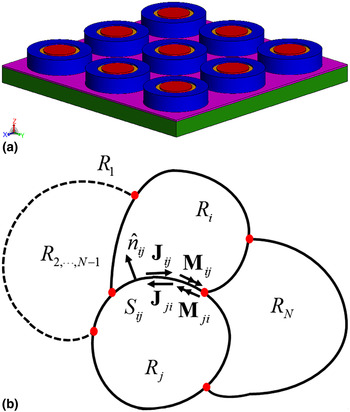
Figure 1(a) illustrates the partial view of a typical functional plasmonic array structure. It is composed of complex building blocks on a layered substrate. Different types of materials with and without dispersion are involved. The array is large and not periodic in general. To solve such substrate-supported plasmonic array problem we consider the configuration as an arbitrary structure consists of many piecewise homogeneous penetrable objects in a homogeneous medium. These piecewise homogeneous regions are denoted by R i , i = 1, …, N, and excited by the time harmonic electromagnetic waves with time factor e jωt , as shown in Fig. 1(b). The material permittivity and permeability parameters of each region are denoted by ε i and μ i .
(a) A general model of substrate-supported plasmonic array, different types of materials are distinguished with different colors. (b) An electromagnetic model of arbitrary shaped substrate-supported plasmonic array consists of N piecewise homogeneous penetrable objects, denoted by R
i
, i = 1, …, N. S
ij
is the boundary surface of regions R
i
and R
j
,
 ${\hat n_{ij}}$
is the unit normal vector of S
ij
.
 ${\bf J}$
and
 ${\bf M}$
are the equivalent surface electric and magnetic currents on the boundaries.

In each region, the electric and magnetic current combined field integral equation (JMCFIE)[ Reference Ansari-Oghol-Beig and Mosalaei 18 ] is applied for these homogeneous penetrable objects. We denote S ij the interface between regions R i and R j , the JMCFIE can specify the total field balance on this surface as
 $${\rm EFI}{{\rm E}_i} + {\eta _i}{\hat n_{ij}} \times {\rm MFI}{{\rm E}_i} + {\rm EFI}{{\rm E}_j} + {\eta _j}{\hat n_{\,ji}} \times {\rm MFI}{{\rm E}_j}{\rm,} $$
 $${\hat n_{ij}} \times {\rm EFI}{{\rm E}_i} + {\eta _i}{\rm MFI}{{\rm E}_i} + {\hat n_{ji}} \times {\rm EFI}{{\rm E}_j} + {\eta _j}{\rm MFI}{{\rm E}_j}{\rm,} $$
where the electric field integral equation (EFIE i ) and the magnetic field integral equation (MFIE i ) can be written as follows:
 $$\eqalign{& \sum\limits_{k \in {C_i}} {{{({\eta _i}{L_i} ({{\bf J}_{ik}}{\rm )} - {K_i} ({{\bf M}_{ik}}{\rm ))}}_{{\rm tan}}}} \cr & \quad + \displaystyle{1 \over 2}{{\hat n}_{ij}} \times {{\bf M}_{ij}} ({\bf r}{\rm )} = {\left( {{\bf E}_i^{{\rm inc}} ({\bf r}{\rm )}} \right)_{{\rm tan}}}{\rm,} \,{\rm} {\bf r} \in {S_{ij}}{\rm,}} $$
 $$\eqalign{& \sum\limits_{k \in {C_i}} {{{\left( {{K_i} ({{\bf J}_{ik}}{\rm )} + \displaystyle{1 \over {{\eta _i}}}{L_i} ({{\bf M}_{ik}}{\rm )}} \right)}_{{\rm tan}}}} \cr & \quad - \displaystyle{1 \over 2}{{\hat n}_{ij}} \times {{\bf J}_{ij}} ({\bf r}{\rm )} = {\left( {{\bf H}_i^{{\rm inc}} ({\bf r}{\rm )}} \right)_{{\rm tan}}}{\rm,} \quad {\bf r} \in {S_{ij}}{\rm.}} $$
Here
 ${\hat n_{ij}}$
is the unit normal vector of S
ij
pointing toward region R
i
, η
i
denotes the wave impedance, and C
i
represents the collection of regions sharing common boundaries with R
i
.
 ${\bf E}_i^{{\rm inc}} ({\bf r}{\rm )}$
and
 ${\bf H}_i^{{\rm inc}} ({\bf r}{\rm )}$
are the corresponding incident electric and magnetic fields. The operators L
i
and K
i
in region R
i
are defined as
 $$\eqalign{ {L_i}({{\bf X}_i})&=j{k_i}\int\limits_S {{{\bf X}_i}({{\bf r}^{\prime}}){G_i}({\bf r},{{\bf r}^{\prime}})d{S^{\prime}}} \cr & \quad - \displaystyle{1 \over {\,j{k_i}}}\nabla \int\limits_S {{\nabla ^{\prime}} \cdot {{\bf X}_i}({{\bf r}^{\prime}}){G_i}({\bf r},{{\bf r}^{\prime}})d{S^{\prime}}},} $$
 $${K_i} ({{\bf X}_i}{\rm )} = PV\int\limits_S {{{\bf X}_i} ({\bf r^{\prime}}{\rm )} \times \nabla {G_i} ({\bf r},{\bf r^{\prime}}{\rm )}dS^{\prime}} {\rm,} $$
where
 ${\bf X}$
represents the unknown
 ${\bf J}$
and
 ${\bf M}$
, K
i
is the wave number, and G
i
is the Green's function in region R
i
with the definition of,
 $${G_i} = \displaystyle{{{e^{ - j{k_i}\left \vert {{\bf r} - {\bf r^{\prime}}} \right \vert}}} \over {4\pi \left \vert {{\bf r} - {\bf r^{\prime}}} \right \vert}} {\rm.} $$
In a similar way, we can get EFIE
j
and MFIE
j
in region R
j
. For the sources
 ${{\bf X}_{ij}} ({\bf r'}{\rm )}$
or
 ${{\bf X}_{\,ji}} ({\bf r'}{\rm )}$
on the interface S
ij
, the boundary conditions enforce the continuity for the tangential components of the fields and imply that
 ${{\bf X}_{ij}} ({\bf r'}{\rm )} = - {{\bf X}_{\,ji}} ({\bf r'}{\rm )}$
.
In this paper, we use curvilinear biquadratic quad elements for the geometry discretization, which substantially reduce number of unknowns in the problem.[ Reference Ansari-Oghol-Beig and Mosalaei 18 ] On these biquadratic quad elements, surface basis functions of order p are defined in the form of
 $${\bf X} = \displaystyle{1 \over {\left \vert {\rm J} \right \vert}} \left( {{{\bf X}_u} (u{\rm,} \;v{\rm )}\displaystyle{{\partial {\bf r}} \over {\partial u}} + {{\bf X}_v} (u{\rm,} \;v{\rm )}\displaystyle{{\partial {\bf r}} \over {\partial v}}} \right){\rm,} $$
where
 ${{\bf X}_u}$
and
 ${{\bf X}_v}$
are order p Legendre and integrated Legendre polynomials, |J| is the determinant value of the Jacobian matrix associated with space mapping between reference and physical elements. It is worth mentioning that the rotated div-conforming basis functions are used in the Garlerkin's test, due to the presence of the
 $\hat n \times $
terms in the JMCFIE in Eqs. (1) and (2). After testing we can get the final system equation Ax = b, A is the impedance matrix, b is the excitation vector, and x is the unknown coefficients vector to be solved.
Domain decomposition method
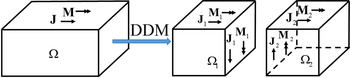
The core idea of DDM is decomposing an original problem into numbers of smaller subdomains, in which the subdomains are solved independently by considering the coupling between subdomains. The concept of DDM is shown in Fig. 2, where the object is partitioned into two subdomains for simplicity.
The illustration of DDM, the object is partitioned into two subdomains for simplicity. After applying the DDM, new unknowns are introduced on the cutting surface, the boundary condition
 ${{\bf X}_{ij}} = - {{\bf X}_{\,ji}}$
is forced to create a powerful transmission condition between adjacent subdomains.

After the whole structure is divided into subdomains, new cutting surfaces appear, and the new unknown electric and magnetic currents should be taken into consideration. Although these subdomains are solved independently, in order to create a powerful transmission condition between adjacent subdomains, the unknown sources
 ${{\bf X}_{ij}}$
(electric or magnetic current) on the interface of subdomains Ω
i
and Ω
j
are forced by the boundary equations
 ${{\bf X}_{ij}} = - {{\bf X}_{\,ji}}$
. This ensures the continuity of the currents around the adjacent surfaces.[
Reference Li and Chew
19
] After applying the DDM, for an N-subdomains system the original system equations Ax = b will be changed into the following form:
 $$\left[ {\matrix{ {{{\rm A}_{11}}} & {{{\rm A}_{12}}} & \cdots & {{{\rm A}_{1N}}} \cr {{{\rm A}_{21}}} & {{{\rm A}_{22}}} & \cdots & {{{\rm A}_{2N}}} \cr \vdots & \vdots & {{{\rm A}_{ij}}} & \vdots \cr {{{\rm A}_{N1}}} & {{{\rm A}_{N2}}} & \cdots & {{{\rm A}_{NN}}} \cr}} \right] \times \left[ \matrix{{x_1} \hfill \cr {x_2} \hfill \cr \vdots \hfill \cr {x_N} \hfill} \right] = \left[ \matrix{{b_1} \hfill \cr {b_2} \hfill \cr \vdots \hfill \cr {b_N} \hfill} \right],$$
where A ij are subdomain impedance matrices. They are self-subdomain interaction matrices for i = j, and the coupling interaction matrices between subdomains i and j for i ≠ j. x i and b i are the unknown coefficients and excitations of subdomains Ω i , respectively.
Fast algorithms
In this work, an IE-FFT solver is applied to solve such DDM matrix system.[ Reference Ansari-Oghol-Beig and Mosalaei 18 ] Most of the IE acceleration techniques, including the IE-FFT method, have inherent assumptions that divide the impedance matrix A into two parts, near-field (NF) interactions and far-field interactions (FF). In metamaterial array design, the building blocks are often required to be a fraction of wavelength with deep-subwavelength features. Thus, a significant part of the system interactions occurs in the NF region. In this paper, we define self-couplings of each building blocks and couplings between the adjacent building blocks as NF interactions. For each building block in a two-dimensional (2D) array, there are at most 32 = 9 near interactions. All the near interaction matrices A ij in Eq. (9) are subject to the low-frequency condition that allows for efficient compression using hierarchical matrix compressed representation, which can bring great reduction of computational time and memory requirement.[ Reference Börm, Grasedyck and Hackbusch 11 , Reference Ansari-Oghol-Beig and Mosalaei 18 ] The couplings between non-adjacent building blocks are defined as FF interactions. The FFT acceleration is used to reduce the cost associated with handling of matrices arising from IE methods.[ Reference Seo and Lee 10 ] A three-level Toeplitz matrix is often used in the traditional FFT-based accelerative method. However, the traditional IE-FFT method always has the accuracy loss problem for NF interaction. To overcome this problem, a six-level Toeplitz matrix instead of the conventional three-level Toeplitz matrix is used to improve the efficiency of IE-FFT in this paper,[ Reference Ansari-Oghol-Beig and Mosalaei 18 ] as the former one eliminates the need for NF correction.
A validation example
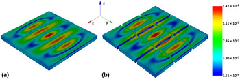
In this subsection, a dielectric slab with the geometric size of 3 × 3 × 0.2 μm3, respectively, along x, y, and z-directions is considered to validate the efficiency of DDM, as shown in Fig. 3(a). A normally incident plane wave with the x-axis polarization at the frequency 100 THz is considered as the excitation, the relative permittivity and permeability of dielectric slab is ε r = 12.5 and μ r = 2.5 (to consider a general case). When DDM is used, we divided this dielectric slab into nine small dielectric slabs with same geometric size, as shown in Fig. 3(b). These nine subdomains are distributed separately in the figure for a better view of each subdomain. It can be observed that the current distributions are the same for the solutions with and without DDM. Also it should be mentioned that 4 min and 1.5 Gb memory are required for the DDM solution, but 2 h and 3.7 Gb memory are required for a direct solution without DDM. This is a speed improvement by a factor of 30. These results are all computed on a personal computer with AMD FX-8120 8-core CPU. Therefore, it can be concluded that the DDM solution can bring a grate reduction both in CPU time and memory requirement without lose any accuracy.
Surface current distribution of a dielectric slab with the geometric size of 3 × 3 × 0.2 μm3 respectively along the x, y, and z-directions, illuminated by a normally incident plane wave at the frequency of 100 THz, (a) without DDM, (b) DDM, the relative permittivity and permeability of dielectric slab is ε r = 12.5 and μ r = 2.5.

Numerical simulation for large plasmonic arrays
In this section, we use surface integral equation (SIE) combined with the IE-FFT accelerative algorithm and DDM to characterize some interesting large plasmonic array platforms. The working scheme of DDM is detailed in the examples by examining the surface current at the subdomain boundaries, and the strategy of dividing subdomains is discussed. The defects with various forms in the large array is easily taken into account and successfully modeled. We start from a geometry which is a large and random hybrid crystal array without substrate, and then we select a rod array with connected substrate to demonstrate the effectiveness of DDM. The third example is a patch antenna array, also with connected substrate, but the substrate permittivity changes from one block to another, where DDM is applied in both vertical and in-plane directions.
The code implementation of the proposed scheme is in C/C++, also the OpenMP parallelization is used for speeding up the computation. All the numerical results are computed on the NEU Discovery cluster.[ 20 ] A Krylov subspace iterative method, Generalized Conjugate Residual[ Reference Carvalho, Gratton, Lago and Vasseur 21 ] with terminate is adopted for the solution of Eq. (9). The iterations terminate upon arrival at a relative residual of < 1 × 10⁻³ and the subspace dimension is assigned as 30.
Hybrid crystal array
Nanocrystal materials can offer interesting optical and electrical features over nanoscales.[
Reference Diroll, Gordon, Gaulding, Klein, Paik, Yun, Goodwin, Damodhar, Kagan and Murray
22
,
Reference Gordon, Cargnello, Paik, Mangolini, Weber, Fornasiero and Murray
23
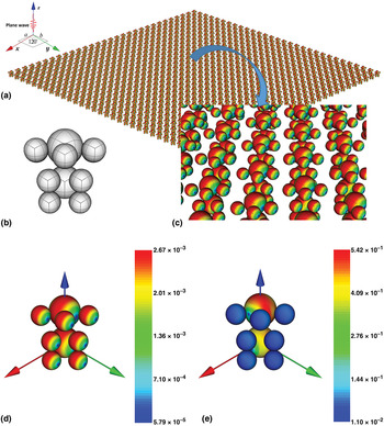
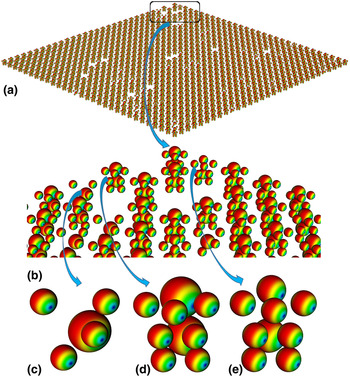
] They are large array and usually made from building blocks of hybrid dielectric and plasmonic elements. Due to fabrication tolerances in size, material and location, the array will not be periodic when it comes to fabrication. Figure 4(a) shows a 30 × 30 crystal array with hexagonal lattice shape. The lattice constants a and b are 30 nm in a xoy −plane with the angle 120°. The building block is composed of two dielectric spheres with diameter 12 nm and seven gold spheres with diameter 7.2 nm, assembling in the shape of hybrid AlB2 and CaCu5 crystal, as shown in Fig. 4(b). Note that the arrangement of the dielectric and plasmonic spheres determines the plasmonic resonances and can be used to engineer the light–matter interaction to our interest. This array is illuminated by a 300 THz plane wave excitation along the minus z-axis direction with the x-axis polarization. The relative permittivity of dielectric and gold spheres at this frequency are ε
rd = 4 and ε
rg = −44.2 − j3.02, respectively, where the relative permittivity of gold is computed based on the Drude model.[
Reference Ashcroft, Mermin and Rodriguez
24
] In Fig. 4(a), the surface electric current densities
 ${\bf J} = \hat n \times {\bf H}$
distribution is shown for the complete crystal array. A zoom in view is given in Fig. 4(c). The high-order curvilinear meshes are shown, in which the high-order basis functions based on Legendre and integrated Legendre polynomials are defined. It is a key of reducing computational cost. Even in single curvilinear patch, we can find the obvious current variation implying that applying high-order basis function brings the inherent benefit of high accuracy. For a better view, the electric current densities
 ${\bf J}$
and magnetic current densities
 ${\bf M} = {\bf E} \times \hat n$
of one building block is shown in Figs. 4(d) and 4(e). We can observe differences in electric and magnetic current densities and for plasmonic and dielectric elements. Such structure provides enough degree of freedom to successfully tailor unique properties by changing the arrangement and the dimensions, for example to create an artificial magnetic current creation, and further to engineer the effective materials parameters.
(a) A 30 × 30 crystal array with lattice constant a = b = 30 nm in a xoy −plane, the angle between a and b is 120°, (b) one building block, consisted of two dielectric spheres with diameter 12 nm and seven gold spheres with diameter 7.2 nm, curvilinear meshes are also shown. (c) A zoom in view of the surface electric current densities
 ${\bf J} = \hat n \times {\bf H}$
, illuminated by a 300 THz plane wave along the minus z-axis direction with the x-axis polarization, also depicting the high-order curvilinear meshes, (d) electric current densities
 ${\bf J} = \hat n \times {\bf H}$
of one building block, and (e) magnetic current densities
 ${\bf M} = {\bf E} \times \hat n$
of one building block.

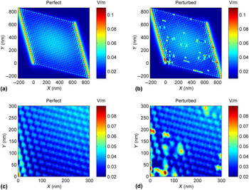
However, the practical fabrication process of the crystal usually leads to imperfections, such as element vacancy, center shift, and deformation. We need to evaluate how these undesired factors may influence the array performance and what is the tolerance of the geometric defects. Thus, it is necessary to take these defects directly into the full-wave simulation. Here 100 building blocks are randomly chosen and changed, in which 35 building blocks have a center shift along the z-axis with 2 nm, 30 building blocks miss parts of the spheres, 20 building blocks are of different sphere radius size and 15 building blocks are completely moved, as shown in Fig. 5. In this paper, we call it perturbed case for the array with defects and perfect case without defects. Figure 6 shows the NF of the perfect and perturbed cases 10 nm away from the top of crystal in a xoy −plane. The comparison in Fig. 6 indicates that the field is obviously changed near the defected building blocks. Strong fields are observed at the vacant lattices due to the cavity-like defect configuration. This information is helpful for designing properly according to the fabrication imperfections.
(a) A perturbed 30 × 30 crystal array, 100 building blocks are randomly chosen and changed, in which 30 building blocks miss parts of the spheres (c), 35 building blocks have a center shift along the z-axis with 2 nm (d), 20 building blocks are of different sphere radius sizes (e), and 15 building blocks are moved, the blank in (b).

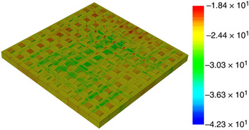
Near electric field distribution 10 nm away from the top of crystal in a xoy −plane, (a, c) the perfect case, (b, d) the perturbed cases, (c, d) are the zoom in view of (a, b) both with the x- and y-coordinate positions between 0 and 300 nm.

The total number of unknowns for the perfect and perturbed crystal array is about 10 and 9.7 million, respectively. Some building blocks are removed or changed in the perturbed case, which explains the different unknown numbers for the two cases. For the perfect case, the total memory and computational time are 36.6 Gb and 2.8 h, respectively, whereas 41.5 Gb and 5.8 h are consumed for the perturbed cases. It is interesting to note that for the perturbed case simulation, though number of unknowns is a little bit less than for the perfect case, the computational cost is actually higher. This is because all the building blocks are the same in the perfect case, an immediate result is that the self-subdomain interaction matrices A ii of Eq. (9) are all the same for each subdomain when DDM is applied and more duplicate information can be used during the matrix setup and solving process. However, comparing with perfect case, more information needs to be computed and stored and this results in higher computational cost for perturbed case. Note that as illustrated with an example in Fig. 3 using a non-DDM for modeling such complex non-periodic configuration will be extremely time-consuming.
Rods array on substrate
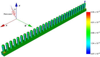
The SiC nanorods can offer surface phonon polaritons with picoseconds lifetime, which is orders of magnitude longer than the scattering time of free carriers in the SPP mode of metals and doped semiconductors.[ Reference Caldwell, Glembock, Francescato, Sharac, Giannini, Bezares, Long, Owrutsky, Vurgaftman, Tischler, Wheeler, Bassim, Shirey, Kasica and Maier 25 ] Figure 7 shows the structure of the second example, SiC nanorod array on top of SiC substrate. Such array may find applications for various wave-front engineering by tailoring the aspect ratio of the rod in a gradient way. The modeling can be challenging as the rods are sitting on a plasmonic substrate, where strong field coupling may happen (and considering the array may not be periodic). Hence, a sophisticated model is needed to solve such large non-periodic highly coupled phenomena.
Electric current distribution on the surface of an SiC array with 30 building blocks, illuminated by a θ-polarized plane wave from θ = 155°, = 90° at the frequency 27 THz.

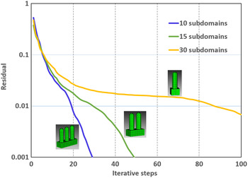
Before simulating the large non-periodic rod array, we would like to show some DDM features for modeling such substrated array structures. An SiC rod array with 30 building blocks along the x-axis direction is taken into consideration, which is illuminated by a plane wave with θ directional polarization from the direction of θ = 155°, φ = 90° at the frequency 27 THz, as shown in Fig. 7. A rod of 800 nm tall and 250 nm diameter on a 400 nm square substrate with the thickness 300 nm is assigned as the building block for this array. Both the rod and the substrate is SiC with the relative permittivity ε r = −5.14 − j0.08. As mentioned in the previous DDM section, the object can be theoretically divided into any number of subdomains. Next we discuss the DDM features for modeling such structure. Three different strategies are used to decompose the 30 building blocks array by putting one, two, and three building blocks in each subdomain, respectively. Thus there are 30, 20, and 10 subdomains for each case. The iterative behaviors of the three different decomposition strategies are summarized in Fig. 8, which imply that the more subdomains we have, the slower the iterative process will be. This means there may be convergence problem for very large-size array if we divide array into too many subdomains. However, the computational statistics in Table I shows that the less memory will be needed if we have more subdomains. This special phenomenon means trade-off relation between iterative steps and memory cost. Therefore some balance between the time and memory cost should be chosen in the DDM design, this is usually determined by the specific simulated structures and hardware computation platforms. It should be mentioned that the substrate has a negative permittivity value and it can support strong NFs, a larger subdomain allows a better performance in DDM. Therefore we put 3 × 3 = 9 building blocks in one subdomain during our following 30 × 30 rod array simulation both considering the computational efficiency and hardware platform limitation.
The iterative behavior of three different decomposition strategies.

Computational statistics for three different decomposition strategies.

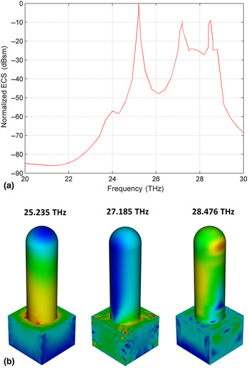
To quickly find the resonance frequency points of the large-scale SiC rod array in the interested band, we compute the extinction cross-section response (ECS) of one SiC rod in the band from 20 to 30 THz in Fig. 9(a). Three resonance frequency points 25.235, 27.185, and 28.476 THz are found. The incident information is the same as the previous case. The dominant resonance happens at 25.235 THz, where the ECS value is very large. The surface electric current density distributions at three resonant frequencies are shown in Fig. 9(b), where strong field coupling is observed at the junctions of the rod and the substrate at the first resonant frequency. This further highlight the capability of the scheme in dealing with highly coupled structures.
(a) The normalized ECS of a single rod with the substrate in the frequency band from 20 to 30 THz, three resonance frequency points 25.235, 27.185, and 28.476 THz are found, (b) surface electric current densities distribution at three deferent frequency points.

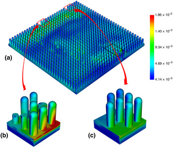
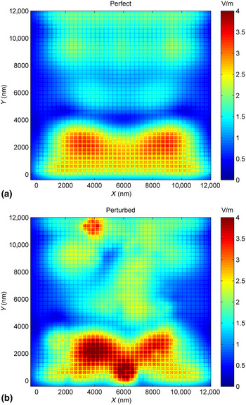
We next perform the defect analysis for the large non-periodic rod array with 30 × 30 building blocks with the similar operation for the hybrid crystal array example. Imagine in the fabrication 50 building blocks have defects and are randomly distributed, among which 30 rods have different heights and radius as shown in Fig. 10(b), the other 20 rods are moved as shown in Fig. 10(c). This is the perturbed case for rod array. Figure 11 shows the NF of the perfect and perturbed cases 100 nm away from the top of rod array in a xoy −plane, in which the fields are obviously changed near the defected building blocks. Due to the randomly changed building blocks, the electric field distribution are not symmetric anymore, also the field intensity have been enhanced in some places.
(a) The surface current distribution on a 30 × 30 rod array (perturbed case), illuminated by a θ-polarized plan wave from θ = 155°, ϕ = 90° at the frequency 25.235 THz, (b, c) surface current distribution on part of the structure, a zoom in view.

Near electric field distribution 100 nm away from the top of rod array in a xoy −plane, (a) the perfect case and (b) the perturbed case.

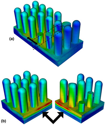
To closely check how DDM works for large substrate-supported array, the black square area in Fig. 10(a) was taken into consideration. We decomposed this area along the dashed square area into two parts, as shown in Fig. 12(a). New cutting surfaces would appear, on which the new electric and magnetic currents emerge. A torn view is shown in Fig. 12(b), where the surface current intensities on the touching surface are the same. This is benefited from the force boundary condition in DDM, also currents are continues on interfaces.
(a) A zoom in view of black square part of in Fig. 10(a), meshes are shown, (b) a torn view when (a) was decomposed along the dashed square area into two parts, new electric and magnetic currents emerged on the cutting surfaces.

The total number of unknowns for the perfect and perturbed rod array is about 4.2 and 4.1 million, respectively. For the perfect case, the total memory and computational time are 155.6 Gb and 26.4 h, respectively, whereas 228.2 Gb and 54.5 h are consumed for the perturbed cases. We can find the same behavior that the computational cost is higher for perturbed case, although the number of unknowns are almost the same or even less. This special behavior has already been analyzed for the crystal array in the last section. It is because more duplicate information is used for the perfect case. Another interesting behavior is that when we compare the computational cost for crystal and rod array, both the computational time and memory requirement for rod array are much higher than for the crystal array, though the number of unknowns is less. This is mainly caused by two factors. The first factor is caused by different decomposition strategies. Both the two arrays have 900 building blocks, but a large subdomain with nine building blocks is employed for the rod array. This results in more subdomains for the crystal arrays and we already get the conclusion that the less memory will be needed if there are more subdomains during the DDM feature testing in the previous section. The other important factor is that the building blocks in the rod array are all touched, so the source and observation elements are not so “well separated”. The efficiency of the hierarchical matrix method strongly relies on low rank compression of matrix blocks associated with simulations.[ Reference Börm, Grasedyck and Hackbusch 11 , Reference Ansari-Oghol-Beig and Mosalaei 18 ] If the source and observation elements are not “well separated”, the compression ratio won't be high, which will increase both CPU time and memory requirement during the computation.
Two-layered substrate patch antenna
A third example we study is the array of gold antennas on the two-layer substrate composed of indium tin oxide (ITO) and SiO2 slabs, where the permittivity of ITO changes from one block to another. This can be achieved by voltage control of the substrate with proper biasing network.[ Reference Esquius-Morote, Gomez-Diaz and Perruisseau-Carrier 16 , Reference Jun, Gonzales, Reno, Shaner, Gabbay and Brener 17 ] This is a promising design idea for application in the area of dynamically tunable array antennas and metasurfaces. Compared with previous structures, the computational difficulty of this design stays in the inhomogeneous permittivity pattern (in a plane). When the DDM is used to model array structures, the whole structure will be divided into many subdomain problems and each domain are solved independently, as shown in Eq. (9), the whole matrix equation is decomposed into numbers of submatrix equations. Therefore for the array with inhomogeneous permittivity pattern, DDM can be applied both for the vertical and in-plane directions, and we can make the permittivity constant in each subdomain. This inherent merit of DDM will greatly reduce the difficulties brought by inhomogeneity.
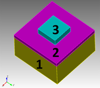
In this section, the plasmonic patch antenna array with the two-layered substrate is considered, one element is shown in Fig. 13, which consists of three different materials denoted as 1, 2, and 3, for the SiO2 substrate, thin-layer ITO with tunable permittivity, and gold antenna. The geometry size of three cuboids are 400 × 400 × 200 nm3, 400 × 400 × 30 nm3, and 160 × 160 × 40 nm3, respectively, along the x, y, and z-directions. A normally incident plane wave with the x-axis polarization at the frequency 167.7 THz (relative permittivity for ITO is −2 − j1.34) is considered as the excitation, the relative permittivity of gold and SiO2 is ε rg = −149 − j 15.8 and ε rd = 3.8. A 10 × 10 plasmonic patch antenna array is simulated, shown in Fig. 14. The relative permittivity of the ITO substrate in each building block is different, varying from ε r = −2 − j 1.34 to ε r = −0.19 − j 0.77, which can be managed for instance with a bias. The number of unknowns in the plasmonic patch antenna array is about 1 million. The total memory and computational time is of 33 Gb and 2.5 h, respectively. One can see despite of the normal incident plane wave the performance of the array is changing from one element to another due to different material substrates. As said earlier our goal here mainly has been to show the power of DDM in solving a in-plane inhomogeneous material, rather than designing a functional system taking all practical aspects into it. It is an obvious extension of this model and to apply to dynamically tunable metasurfaces and antennas,[ Reference Cheng, Wang, Mosallaei and Kaxiras 26 ] which will be the focus of future works.
One plasmonic patch antenna with the two-layer substrate, material 1, 2, and 3 are SiO2, ITO, and gold, respectively. The geometry size of three cuboids are 400 × 400 × 200 nm3, 400 × 400 × 30 nm3, and 160 × 160 × 40 nm3, respectively, along the x, y, and z-directions.

The surface current distribution on a 10 × 10 plasmonic patch antenna array, normally illuminated by an x-axis polarized plane wave at the frequency 167.7 THz.

Conclusion
Despite the great advances achieved to date for the physical concept of efficient wave manipulation in metamaterials and graded plasmonic array systems, it is still a challenging task to model the large plasmonic array platforms without periodicity. In this paper, we proposed a SIE combined with the IE-FFT accelerative algorithm and DDM for solving large substrate-supported plasmonic array problems. Without any periodicity assumptions, results of the surface currents and NF intensity for arrays with hundreds of building blocks and complex element geometry can be computed using the proposed scheme. Three different examples are considered here to show the ability of the model. Large arrays of crystal structure and SiC nanorods on a substrate are numerically modeled. Different types of random defects are introduced based on the fabrication scenario. Without any periodicity assumption, results of the surface currents and NF intensity for large arrays with and without defects are calculated and compared, which can provide valuable guidance for practical fabrication and measurement. Also a plasmonic patch antenna array with a two-layer substrate are designed and presented. Benefited from the features of DDM, we can model the substrate layer with inhomogeneous permittivity distribution changing among subdomains, which can be further implemented by tunable materials. It should be mentioned that all the three structures solved in this paper have large area with millions of unknowns, and such large-size structures can be widely used in practical applications and difficult-time consuming to be modeled with current computational methods. The proposed computational scheme will be of great advantage for fast and accurate modeling of future plasmonic materials and metasystems.
Acknowledgment
This work is supported in part by DARPA award via Grant # N00014-14-1-0850 and in part by AFOSR award Grant # FA9550-14-1-0349. The authors would like to also acknowledge the help of Dr. Davood Ansari-Oghol-Beig and discussion with him during this project.