Parameter selection from thermochemical data

Implementation of parameter selection with only thermochemical data allows the Gibbs-energy models of each phase to be evaluated directly from the data, therefore models for each phase can be generated independently. The construction of the Gibbs energy within the CEF involves the extrapolation of the low order terms in composition into the interaction space, so all endmembers must be fit first, followed by the excess parameters from low order to high order. Interaction parameters are evaluated with candidate models from the zeroth-order to fourth-order interactions, fitting all the temperature dependent terms in a Redlich–Kister polynomial^{[Reference Redlich and Kister23]} for the zeroth-order interaction before fitting all the Redlich–Kister terms for the first-order interaction and so on. ESPEI can currently generate model parameters for binary and ternary systems. Endmember energies and interactions are evaluated in the following sequence, using a hypothetical three sublattice ternary solution phase as a prototype for a phase with v-sublattices and j-components. A three sublattice binary solution phase where A, B, and C can occupy any sublattice is described as (A, B, C) : (A, B, C) : (A, B, C), where each sublattice is separated by a “:”. A “*” is used to denote the presence of any arbitrary component. It should be noted that while cross-sublattice interactions are fit by ESPEI to ensure the generality of the software, it is rare for CALPHAD models to include cross-sublattice interactions.

1. (1) Fit 1-sublattice binary interactions, e.g., (A, B) : * : *

2. (2) Fit binary interactions across two sublattices, e.g., (A, B) : (*, *) : *

3. (3) Fit binary interactions across n sublattices up to the vth sublattice

4. (4) Fit ternary interactions, e.g., (A, B, C) : * : *

5. (5) Fit ternary interactions across two sublattices, e.g., (A, B, C) : (*, *, *) : *

6. (6) Fit ternary interactions across n sublattices up to the vth sublattice

A simple model with few parameters is better than a complex model that describes the same data marginally better. Parameter generation in ESPEI aims to achieve a balance of a simple parameterization and goodness of fit of the model to the data. The polynomial for the Gibbs energy as a function of temperature has the form given in Eq. (1):

(1)$$G = a + b\; T + c\; T\ln T + \mathop \sum \limits_n d_n\; T^n$$

Different parameterization combinations of Eq. (1) are considered, such as a parameterization of only a, only a and b, and so on. The parameters that will be considered are limited by the input thermochemical data and how the derivatives of the Gibbs energy can describe the parameters. In general, candidate models that could not physically describe the underlying Gibbs energy function are not generated. For example, isothermal enthalpy of formation data cannot describe high-order terms of the Gibbs energy, and thus they will not be considered when only enthalpy data are used.

In this polynomial, all the terms are linear with respect to the model coefficients, so the candidate models can be fit to input thermochemical data by a linear least squares optimization under the assumption that the residuals follow a Gaussian distribution. A tunable hyperparameter, α in Eq. (2), controls the weight of the L2 regularization, w ², that penalizes the magnitude of the parameters can be adjusted by the user to prevent overfitting, resulting in the objective function given in Eq. (2), where w is the vector of coefficients, X is the matrix of polynomial terms, and y is the data to be fit.

For each fitting step, the parameters for the candidate models are evaluated by minimizing Eq. (2), then the residual sum of squares (RSS) between the evaluated parameters and the data are used to score and compare the models within the corrected Akaike information criterion (AICc).^{[Reference Cavanaugh24]} The model with the lowest score is the optimal combination of model fitness and complexity. The AICc is a modified version of the AIC^{[Reference Akaike25]} that avoids overparameterization when the data are sparse, which is often the case for thermochemical data. The AICc score is calculated by Eq. (3), where k is the number of parameters, n the number of samples, and RSS is the residual sum of squares between the model predictions and the data. In this way, models for each phase with a reasonable fit/complexity tradeoff can be built up one parameter at a time.

(2)$$O = \lpar {Xw-y} \rpar ^2 + \alpha w^2$$

(3)$${\rm AICc} = {\rm AIC} + \displaystyle{{2k^2 + 2k} \over {n-k-1}} = 2k-n\ln \displaystyle{{{\rm RSS}} \over n} + \displaystyle{{2k^2 + 2k} \over {n-k-1}}$$

Parameter optimization to phase equilibria data

The CEF uses sublattices to describe the chemical behavior of occupancy and substation of elements on sublattices, typically representing the Wyckoff positions in crystalline materials. The endmembers that the CEF introduces into the Gibbs-energy model are often not stable or cannot be characterized completely experimentally due to the high dimensionality of the sublattice composition space that is not directly accessible by experiments. Measurements of the Gibbs energy derivatives in CEF models cannot be obtained completely from experiments in the general case, requiring the use of thermodynamic data indirectly related to the Gibbs energies of the phases to refine the parameters generated from thermochemical data to construct a self-consistent set of parameters that reproduce the known data for a given system. In many practical binary and ternary systems of interest, a typical CALPHAD description might have on the order of tens to hundreds of parameters to assess. Current optimization methods require modelers to restrict the degrees of freedom to only a handful of simultaneous parameters and optimize the restricted sub-problems iteratively.

Bayesian parameter estimation is a method of optimizing model parameters by Bayes theorem,^{[Reference Gelman, Stern, Carlin, Dunson, Vehtari and Rubin18]} obtaining the posterior probability, p(θ|D), of the model parameters, θ, conditioned on the data, D, in Eq. (4). The prior, p(θ), contains the domain knowledge of the modeler in the probability distribution of each parameter. The likelihood, p(D|θ), is the probability that the data are described by a set of parameters, and evidence, p(D), is the probability of the data marginalized over the possible parameters. In CALPHAD databases, evaluating a closed form solution for these quantities over all model parameters is not computationally achievable, so the posterior probability is determined numerically using MCMC:

(4)$$p(\theta \vert D) = \displaystyle{{\,p(\theta )p(D{\rm \vert} \theta )} \over {\,p(D)}}$$

ESPEI uses MCMC to perform Bayesian parameter estimation on all model parameters simultaneously. In principle, MCMC optimization in ESPEI can be performed for arbitrarily sized multicomponent, multiphase systems with any number of degrees of freedom, however this is not computationally feasible in practice and it is expected that the extrapolation of binary and ternary CALPHAD parameters into multicomponent space precludes the need to model all the degrees of freedom in a multicomponent system simultaneously. However, a challenge in applying MCMC to optimize parameters in CALPHAD databases is that most MCMC samplers assume that model parameters are uncorrelated with efficiently explore parameter space.^{[Reference Gelman, Stern, Carlin, Dunson, Vehtari and Rubin18]} The parameters in CALPHAD models for each phase are correlated with each other because increasing the value of one parameter and decreasing that of another can give the same Gibbs energy for any given set of conditions. This challenge is addressed in ESPEI by using an ensemble sampler, as introduced by Goodman and Weare.^{[Reference Goodman and Weare26]} Ensemble samplers use an ensemble of Markov chains to form the proposal distribution for the parameters. This allows the proposals to be invariant under affine transformations, solving the problems of scaling proposal length and differing parameter magnitudes in multidimensional parameter space simultaneously. Proposed parameters are accepted or rejected based on the Metropolis criteria, Eq. (5). The probability of accepting a step is given in Eq. (5), where p _current = p(θ_i)p(D|θ _i) is the probability for the current set of parameters and p _proposed = p(θ_i+1)p(D|θ _i+1) is the probability for the newly proposed parameters. Thus, the Metropolis criteria accepts all proposed parameters that increase the probability, i.e., p _proposed/p_current >1 so p _accept = 1, but there's also a p _proposed/p _current chance of accepting parameters that decrease the probability accepts proposals that decrease the posterior probability. The ability to accept parameters that decrease the probability leads to the convergence of the probability to the true posterior distribution:

(5)$$p_{{\rm accept}} = {\rm min\;} \left( {\displaystyle{{\,p_{{\rm proposed}}} \over {\,p_{{\rm current}}}},{\rm \;} 1} \right)$$

Adding parameters that decrease the posterior probability to the Markov chain systematically constructs the posterior distribution from the point estimates of the probability density. ESPEI uses an ensemble sampler algorithm implemented in the emcee package^{[Reference Foreman-Mackey, Hogg, Lang and Goodman27]} that implements parallelizable ensemble samplers. ESPEI provides emcee with an initial ensemble of chains as Gaussian distributions centered on the parameters generated by single-phase fitting and defines a probability function that calculates point posterior log-probabilities from the prior and likelihood. Log-probabilities are often used in MCMC software to prevent floating point errors when multiplying probabilities. It should be noted that ESPEI can fit parameters for any type of model in a TDB if the individual model parameters can be specified using the FUNCTION command in the TDB format.^[28]

Prior distributions for the parameters are the main way that modelers input domain knowledge into ESPEI's MCMC optimization. Each parameter has a probability density function associated with it that, for a given set of parameters, can be used to evaluate p(θ). Often the same type of prior distribution is used for each parameter, but this is not a requirement. Any function can be used in ESPEI, though there are three prior distribution functions that are easy to use in ESPEI: a uniform, normal, or triangular prior. For convenience, ESPEI provides a method for describing the hyperparameters for these distributions relative to the parameters in the initial database. Uniform priors are uninformative, giving constant probability between upper and lower parameter bounds and are useful when there is low confidence in the initial database parameters. Normal priors follow a Gaussian distribution, usually centered on the parameter. Normal priors are useful for informing a centrality of each parameter in the prior, but not explicitly limiting the parameter bounds. Triangular priors are particularly useful for modeling in ESPEI, as they allow the modeler to inform the centrality of the parameters, e.g., from parameter selection, but also to enforce bounds where the prior probability is zero outside of those bounds, which can be used to ensure that parameters remain with the same sign or within the same order of magnitude, for example. The hyperparameters to generate the prior distributions are specified in ESPEI input files. A detailed example and further explanation are included in the ESPEI software documentation.^{[Reference Bocklund29]}

Three main types of data are considered by the likelihood function defined in ESPEI: single-phase thermochemical data of the temperature derivatives of the Gibbs energy, activity data, and multi-phase equilibria data. All data used in ESPEI are stored as JSON^[30] files with a custom schema defined and validated by ESPEI. For examples of the schema and how data are stored see the supplemental text with the ESPEI manual or the most recent documentation online.^{[Reference Bocklund29]} To ensure consistent weighting of error from different data types, the likelihood for each type of data is normalized by the standard deviation of the error for that data type. For all data types, the error is assumed to follow a normal distribution. ESPEI provides default values for the standard deviations of each type of data, however users can modify the values by adding a weight for each type of data or for each individual dataset. It is important to note that the quality of the standard deviation for each data point is closely linked to the quality of the evaluated uncertainty. Significant effort should be made to use appropriate estimates for uncertainty where the experimental uncertainty is not available. The thermodynamic quantities for each type of data are determined in ESPEI by using pycalphad^{[Reference Otis and Liu17]} as the thermodynamic calculation engine.

The error due to thermochemical data is calculated by comparing the difference between the predicted values and the measured or calculated values. Since these values are calculated or measured directly, the standard deviations of the error are relatively well defined. The default standard deviations for enthalpy, entropy, and heat capacity data are chosen to be 500 J/mol, 0.2 J/K mol, and 0.2 J/K mol, respectively. To fit activity data, the measured activity is converted to chemical potentials as suggested by Lukas et al.^{[Reference Lukas, Fries and Sundman31]} The error is calculated by the difference between calculated and measured chemical potentials. Although activities are not measured directly, the experimental errors are mathematically related to the activity and the experimental errors reported in the literature can be propagated to the chemical potentials, ESPEI chooses a standard deviation in the chemical potential due to measured activity data of 500 J/mol.

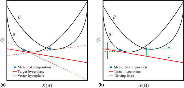
Thermodynamic assessments are judged, to the first order, by the agreement with the measured phase equilibria on the phase diagram, so any complete thermodynamic assessment program must consider optimization of phase equilibria data. The phase equilibria depend on solving for the global minimum energy for many phases and arbitrary models of the Gibbs energy, so a solution mapping the model parameters to the calculated equilibria is not well defined. Several methods exist for determining the error for phase equilibria. The direct approach is to calculate the phase equilibria and determine the error in the phase boundary due to a difference in temperature or composition. However, a drawback of the direct approach is that the phase equilibria of interest are not always stable and a near-optimal solution must already be known to properly calculate the error. Since MCMC optimization considers many degrees of freedom and the initial database may not be close to a globally optimal solution, a more generic approach is warranted. The method implemented by ESPEI is similar to the rough search method implemented in PanOptimizer software.^{[Reference Cao, Chen, Zhang, Wu, Yang, Chang, Schmid-Fetzer and Oates2]} The core concept of this method is to determine driving force of the known stable phase at the measured composition of the zero-phase fraction line, controlling the temperature and pressure. Because the metric used to evaluate the error is the driving force, any method that can measure a zero-phase fraction boundary can be used, such as the transition temperature at a fixed composition measured by, for example, differential scanning calorimetry. The driving force will be zero in the limit of convergence. Given a set of measured phase constitutions in equilibrium (e.g., from EPMA), referred to as tie-line vertices, and a set of candidate parameters for a model the multiphase error can be calculated as follows (illustrated schematically in Fig. 1):

1. (1) Construct the target equilibrium hyperplane as the mean of the equilibrium hyperplane at each tie-line vertex. For each measured tie-line vertex, perform an equilibrium calculation at that set of composition, temperature and pressure conditions with all phases active. The vertex hyperplanes for each tie-line vertex are represented as dashed lines in Fig. 1(a). The target hyperplane is the arithmetic mean of the calculated chemical potentials, shown as a solid line in Fig. 1(a).

2. (2) Compute the single-phase Gibbs energy of each tie vertex, G ^t, with only the desired phase active, shown as the blue points in Fig. 1(b).

3. (3) The residual is the sum of driving forces, calculated as $G^t-\mathop {\sum\nolimits_i {{\bar{\mu}} _ix_i}} \limits_{} $ , where $\bar{\mu} _i$ is the chemical potential of the target hyperplane calculated in step 1.

Figure 1.

Schematic procedure for calculating the error in phase equilibrium data. α and β are Gibbs-energy curves for hypothetical phases. The blue points represent measured phase constitutions projected onto the Gibbs-energy curves. The solid red line represents the target hyperplane as the arithmetic mean of the hyperplanes for the vertex hyperplanes corresponding to each tie-line point [red dashed lines in (a)]. The driving force error (b) is the difference between the target hyperplane and the Gibbs energy at each vertex.

This approach is advantageous because it generalizes well to multicomponent systems and can be used even when the measured phases in equilibrium are not in the calculated stable equilibrium, however there are some special cases that must be considered. It is sometimes the case, especially in binary systems, that the equilibrium phase boundary compositions are unknown for some tie vertices, such as solidus and liquidus boundaries determined by heating and cooling curves. These unknown compositions are excluded from the determination of the target hyperplane. If a stoichiometric compound is found as the only phase in equilibrium when determining the target hyperplane, the chemical potentials must be excluded from determining the target hyperplane because they are not well defined. Using the prior and likelihood functions ESPEI calculates the probabilities for a proposed set of parameters and through MCMC, the posterior probability distributions for each parameter that maximize the probability that the models describe the experimental and calculated data.

Unary reference data

The SR model^{[Reference Roslyakova, Sundman, Dette, Zhang and Steinbach5]} is one of the alternative physically-based formulations to the recently used SGTE description of reference data for pure elements. The SR model has been developed for the description of temperature dependence in the heat capacities down to 0 K considering relevant physical effects and it consists of three terms:

(6)$$ \eqalign{ & C_{\rm P}\lpar {T,{\vector \theta}} \rpar = \displaystyle{{9N_{\rm A}k_{\rm B}} \over {{\lpar {\theta_{\rm D}/T} \rpar }^3}}\int_0^{\theta _{\rm D}/T} {\displaystyle{{x^4{\rm e}^{x}} \over {{(1-{\rm e}^{x})}^2}}{\rm d}x} \cr &+ \left\{ \matrix{ \hskip -6.5pc \beta_1T,{\rm} & T \lt \alpha -\gamma \hfill \cr \beta_1T + \beta_2\displaystyle{{{(T-\alpha + \gamma )}^2} \over {4\gamma}}, & {\rm} \alpha {\rm -} \gamma \le T \le \alpha + \gamma \hfill \cr \hskip -2pc \beta_1T + \beta_2(T-\alpha ), & {\rm} \alpha + \gamma \lt T \hfill} \right. + C_{\rm P}^{{\rm magn}}, $$

where ${\vector \theta} = (\theta _{\rm D},\beta _1,\beta _2,\alpha, \gamma )$ is the vector of unknown model parameters to be estimated from experimental and computational data. Here, the main contribution to the heat capacity due to phonon vibration is represented by the well-known Debye model. The second term in Eq. (6) is a so-called bent-cable model. This term is introduced for the decomposition of linearly-dependent physical effects at low and high temperatures. The last term describes the magnetic contributions to the heat capacity. This term is not considered and equal to zero for non-magnetic elements.

Since the analytical formulation of the Debye model cannot be implemented directly in the TDB format, a non-series approximation of the Debye model base on the weighted linear combination of Einstein functions for heat capacity has been developed to overcome this issue and it has been successfully applied for the thermodynamic re-evaluation of the Cr–Nb system^{[Reference Jiang, Zomorodpoosh, Roslyakova and Zhang39]} and agrees well with available experimental data over the entire temperature range.

The Gibbs energy function for reference data is derived based on the well-known thermodynamic relationship between heat capacity and Gibbs energy:

(7)$$G\lpar T \rpar = \int C_{\rm P}\lpar T \rpar -T\int \displaystyle{{C_{\rm P}\lpar T \rpar } \over T}{\rm d}T\; $$

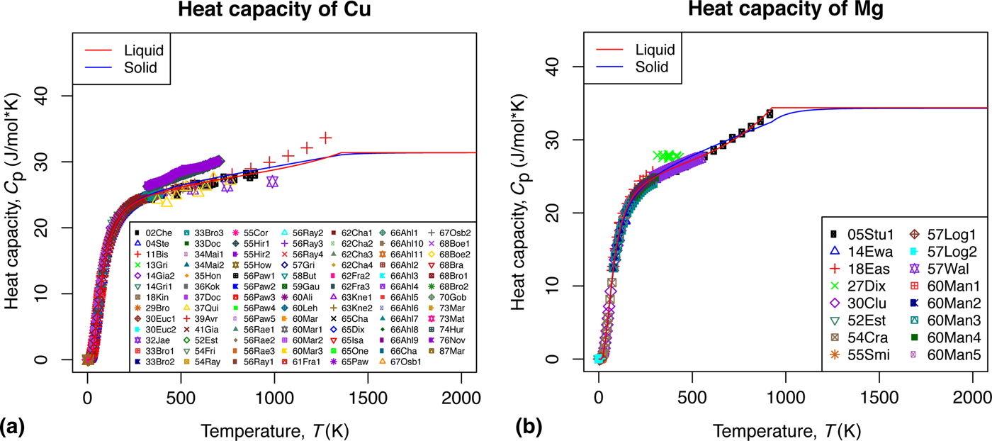
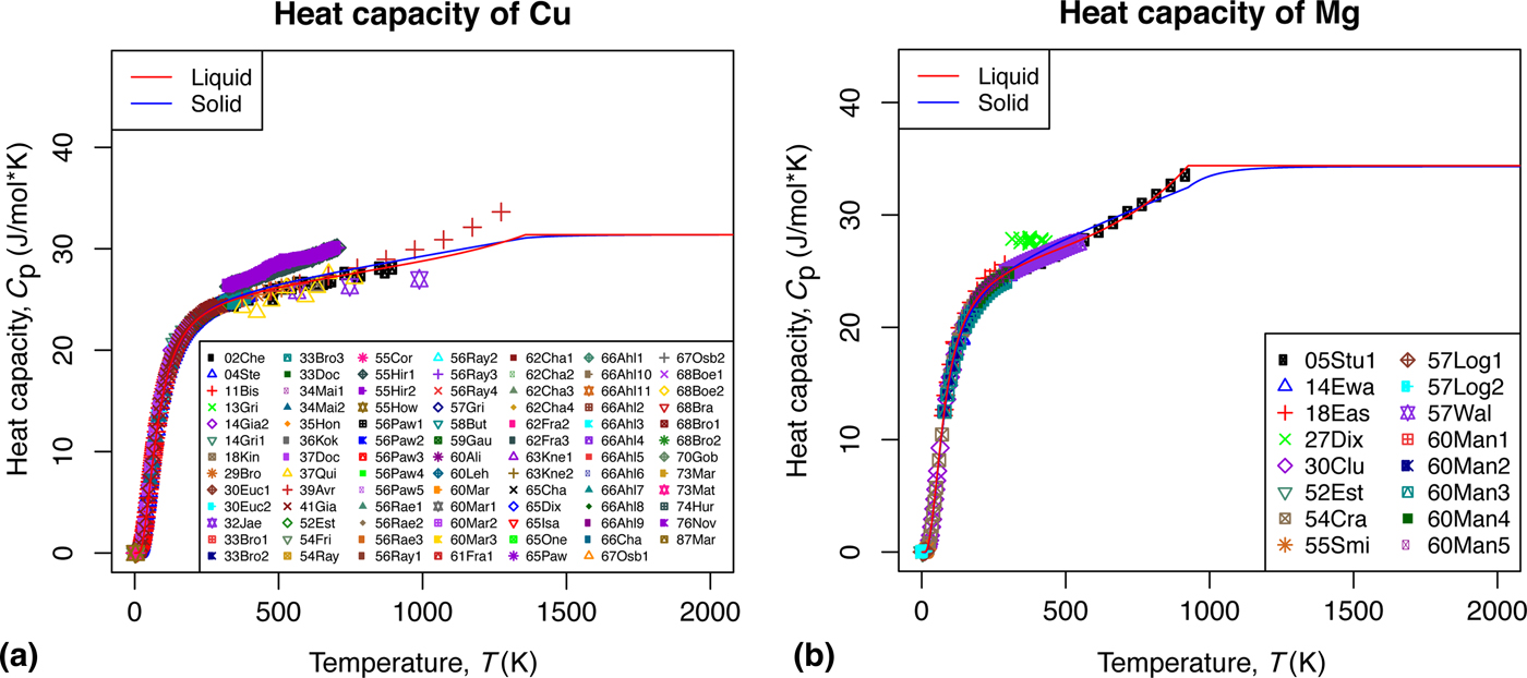
The Gibbs energies were fit for fcc Cu and hcp Mg using this model with the heat capacities for Cu and Mg presented in Figure 2 showing good agreement with experimental data from 0 K up to the melting point. The liquid phase was described using re-assessed coefficients of the SGTE description from room temperature to the melting point. The parameters of the Gibbs energy for the liquid phases were adjusted to have the same relative energy between the solid and liquid phases as the SGTE description. The Gibbs energy below room temperature was extended down to 0 K using a combination of fitted coefficients to the solid phase and three additional polynomial parameters included to guarantee a smooth connection of these two description at room temperature. The lattice stability of the solid phases is the same as the SGTE description for both Cu and Mg. At the time of writing, ESPEI does not support fitting unary descriptions of pure elements and by default does not adjust the unary model parameters in the MCMC optimization. Therefore, the uncertainty in different unary descriptions cannot yet be propagated into the binary and higher order systems that ESPEI assesses.

Figure 2.

Heat capacity of the optimized SR unary models for Cu (a) and Mg (b) compared to the data available in the NIST metals data repository.^{[Reference Wilthan, Pfeif, Diky, Chirico, Kattner and Kroenlein40,Reference Pfeif and Kroenlein41]}

ESPEI optimization

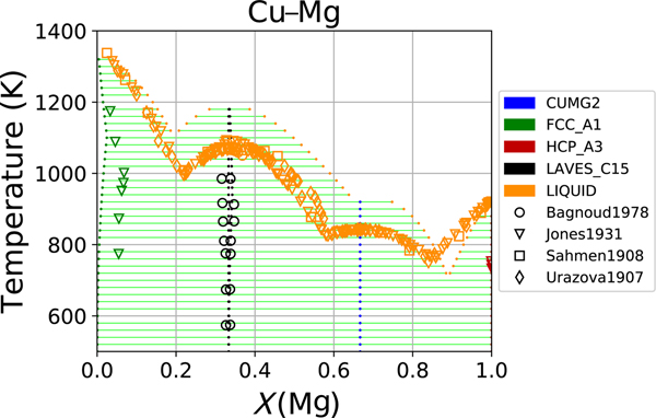
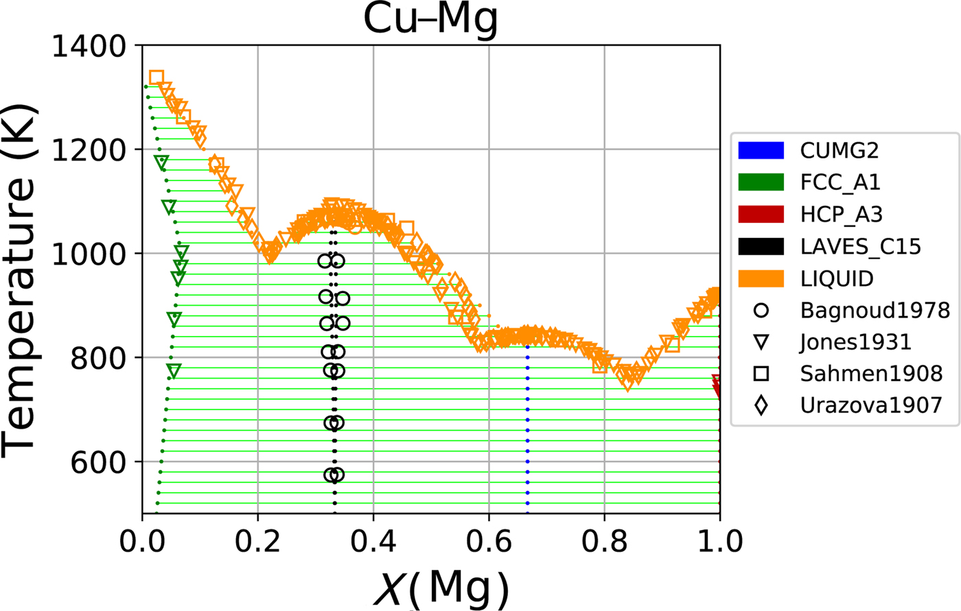
Parameters were generated for the Cu–Mg system based on the measured and calculated single-phase thermochemical data. Experimental enthalpy of formation for the CuMg₂^{[Reference Feufel and Sommer42,Reference King and Kleppa43]} and Laves C15^{[Reference Feufel and Sommer42,Reference King and Kleppa43]} phases and experimental enthalpy mixing for the liquid phase^{[Reference Batalin, Sudavtsova and Mikhailovskaya44]} were used. First-principles calculations for the mixing energies for the FCC_A1 and HCP_A3 phases were calculated by Shin^{[Reference Shin45]} and Gao et al.,^{[Reference Gao, Wang, Shang, Liu, Du and Liu46]} while the endmembers of the Laves phase and CuMg₂ phase were calculated by Zhou et al.^{[Reference Zhou, Wang, Shi, Sommer, Chen, Liu and Napolitano36]} In total, 15 degrees of freedom were generated for the endmembers and binary interactions for the five phases. The resulting phase diagram is shown in Fig. 3. This phase diagram, produced only from the thermochemical data, shows the qualitative behavior of the measured phase equilibria, even though those data were not included in the optimization. The parameters that produced this phase diagram were used as input for the MCMC optimization step with triangular priors that spanned from ± 0.5θ. All the available thermochemical, activity and phase equilibrium data were considered, and all parameters fit to the data simultaneously. Figure 4 shows the phase diagram after 500 MCMC iterations and shows excellent agreement with the phase equilibria data.

Figure 3.

Cu–Mg phase diagram as fit by parameter selection and compared to experimental phase equilibrium data.

Figure 4.

Cu–Mg phase diagram compared to experimental phase equilibrium data after MCMC fitting with all data considered simultaneously.

Uncertainty quantification

CALPHAD-type calculations could consider parameter uncertainty and propagated uncertainty. Parameter uncertainty concerns the distribution of each parameter in a model, while propagated uncertainty is the parameter uncertainty that has been carried through to the uncertainty in different thermodynamic properties that may be calculated. Individual parameter uncertainties are usually not of interest in isolation because the parameters and uncertainties usually are marginalized across several CALPHAD parameters and models as contributions to the Gibbs energy. Parameter uncertainty is evaluated within the MCMC optimization step of ESPEI by quantifying the distribution of the parameter values that make up each Markov chain. To correctly quantify uncertainty, each chain must be converged. MCMC convergence cannot be proved for arbitrary simulations, however several criteria exist that are indicators of convergence. The application of these indicators is the same in ESPEI as any MCMC simulation and is discussed in detail elsewhere.^{[Reference Gelman, Stern, Carlin, Dunson, Vehtari and Rubin18]}

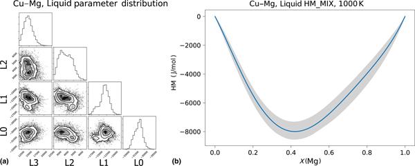
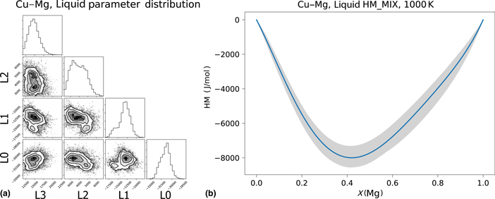
The liquid parameters from the Markov chain constructed in the MCMC optimization are shown in the corner plot in Fig. 5(a). The histograms for each parameter are plotted along the diagonal of the corner plot and the covariance between each pair of parameters is plotted below the diagonal. The histograms of each parameter are not required to follow any distribution because the probability is the product of the likelihood and the prior, which can have varying shape in parameter space. For parameters in CALPHAD models, it is expected that some parameters will exhibit covariance, particularly for parameters in the same phase and between phases in equilibrium. Too many parameters that are correlated are an indication that fewer parameters are required to describe the Gibbs energies that the data require. Uncertainty from the MCMC chains and probabilities were propagated to the enthalpy of mixing in the liquid phase in Fig. 5(b). To propagate the uncertainty, 95% of the parameter values with the highest probability density were used to calculate the target values, forming the 95% highest density intervals (HDI) for each type of data. The mean enthalpy of mixing is plotted as the line, and the 95% HDI is plotted as the shaded region in Fig. 5(b). The uncertainties in the enthalpy of mixing in the liquid region are smaller where liquid is in stable two phase equilibrium on the phase diagram and where the different sets of experiments agree. Near the congruent melting of the Laves phase, there is some disagreement in the data, which leads to a region of relatively larger uncertainty. The maximum uncertainty is on the order of 1 kJ/mol, which is consistent with what would be expected from experiments. Since the unary descriptions are fixed in this optimization, there is no uncertainty bound at either pure Cu or pure Mg will always be 0. Fitting unary parameters in ESPEI would enable the uncertainty quantification. More details on the statistical approach of propagating parameter uncertainty, especially to phase diagrams, is published in a separate article.^{[Reference Paulson, Bocklund, Otis, Liu and Stan47]}

Figure 5.

Corner plot (a) of the parameters in the fcc phase. The diagonal images show the histogram of each parameter in the Markov chain and the off-diagonal images show the covariance between two parameters. Parameter uncertainty propagated to (b) the enthalpy of mixing for the liquid phase. The blue line in (b) is the mean and the gray area is the 95% high density interval.