2.1 Estimating canonical correlations

In practice, the expectations in (1) are replaced by sample-based estimates computed from observation matrices X = [x₁, . . ., x_N] and Y = [y₁, . . ., y_N], resulting in a sample canonical correlation

(2)

Here, C_xy = C_yx^T is a between-sets covariance matrix and C_xx and C_yy are within-sets covariance matrices of the two random variables x and y. Unbiased estimates of the covariance matrices can be obtained by

(3)

where C is the full correlation matrix and N is the sample size.

Since the solution of (2) is not affected by the re-scaling of a or b, the choice of re-scaling is arbitrary, and thus the maximization problem is equal to maximizing the numerator subject to

(4)

As shown by Bach and Jordan (Reference Bach and Jordan2003), CCA reduces to solving the following generalized eigenvalue problem:

(5)

which gives D_x + D_y eigenvalues {ρ₁, −ρ₁, . . ., ρ_D, −ρ_D, 0, . . ., 0}, such that ρ₁ ≥ ρ₂ ≥ . . . ≥ ρ_D. The eigenvectors A = [a₁, . . ., a_D]^T and B = [b₁, . . ., b_D]^T corresponding to D non-zero canonical correlations are the basis vectors for the canonical variates U = [u₁, . . ., u_D]^T = A^TX and V = [v₁, . . ., v_D]^T = B^TY. Furthermore, the canonical variates are orthogonal (UU^T = VV^T = I).

The estimates of canonical correlations depend heavily on the sample size and the dimensionality of random variables. A standard condition in classical CCA is N/(D_x + D_y) ≫ 1. If the ratio is small, the sample covariance matrix C_xy may become ill-conditioned. It leads to a trivial or over-fitted CCA solution with canonical correlation of exactly one. Furthermore, the sample covariance matrices C_xx and C_yy may also be singular or near singular, leading to unreliable estimates of their inverses. One way to solve this issue is to introduce some kind of regularization (Leurgans, Moyeed and Silverman Reference Leurgans, Moyeed and Silverman1993; De Bie and De Moor Reference De Bie and De Moor2003; Hardoon et al. Reference Hardoon, Szedmak and Shawe-Taylor2004) by introducing smoothing to modify the constraints in (4). The regularized variant is solved through the same optimization problem, but a small positive value is added to the diagonal of C_xx and C_yy in the eigenvalue problem.

2.2 Canonical factor loadings

Canonical correlation analysis can be interpreted in terms of canonical factor loadings. In factor analysis, a loading is defined as a simple correlation between a variable and a factor. The square of the loading gives the variance of the variable explained by the factor (Harman Reference Harman1960; Rummel Reference Rummel1970). Canonical factor loadings can be analogously defined as correlations between the original variable (x_j or y_j) and each canonical variate (uuu_i or vvv_i) in both the data sets:

(6)

The loadings measure which variable is involved in which canonical variate and to what extent. Hence, a variable with a large canonical factor loading should be given more weight while deriving the interpretation of respective canonical variate. Moreover, the sum of the squared factor loadings divided by the number of variables in the set is the proportion of variance in the set explained by the given canonical variate. In Section 5.4, we use the factor loadings for manual inspection of the variates.

2.3 CCA's connection to mutual information

There is a simple relationship between canonical correlation and mutual information (MI) for Gaussian random variables (Bach and Jordan Reference Bach and Jordan2003). Given two Gaussian random variables x = [x ₁, . . ., x _{D x}]^T and y = [y ₁, . . ., y _{D y}]^T, the MI, I(x;y) can be written as

(7)

where |.| denotes the determinant of a matrix.

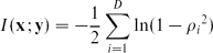
If C_xx and C_yy are invertible, the product of the eigenvalues is equal to the ratio of determinants in (7). Consequently, MI can be written in terms of canonical correlations (Kay Reference Kay1992):

(8)

2.4 Nonlinear extensions to CCA

In many applications, it may not be sufficient to find linear dependence. One way to capture nonlinear dependence using CCA is to allow nonlinear transformations. Several authors (Lai and Fyfe Reference Lai and Fyfe2000; Akaho Reference Akaho2001; Melzer, Reiter and Bischof Reference Melzer, Reiter, Bischof, Dorffner, Bischof and Hornik2001) have presented a CCA extension that enables nonlinear transformations using kernel functions. Kernel canonical correlation analysis (KCCA) has been further studied, for instance, by Bach and Jordan (Reference Bach and Jordan2003) and Hardoon et al. (Reference Hardoon, Szedmak and Shawe-Taylor2004). In KCCA, the correlation matrices are replaced with a kernel function in the dual form. The data are projected into a feature space of high dimensionality H using kernel functions ,

(9)

before computing CCA in the kernel space. Due to the higher dimensionality in the kernel space, KCCA overfits badly. In consequence, proper regularization is crucial for non-trivial learning (Bach and Jordan Reference Bach and Jordan2003; Hardoon et al. Reference Hardoon, Szedmak and Shawe-Taylor2004).

2.5 Applying CCA to language data

Canonical correlation analysis and its variations have already been utilized in many applications of natural language processing. Cross-language IR is one of the applications in which CCA has been applied to a bilingual corpus. Mate retrieval is an IR task in which a document in a source language is used as the query and the corresponding document (‘mate’) in a target language is considered to be the only relevant document to the query. Vinokourov et al. (Reference Vinokourov, Shawe-Taylor and Cristianini2003) use KCCA in mate retrieval task for a sentence-aligned English–French corpus in which the documents are single paragraphs. In their experiments, KCCA performs significantly better than latent semantic indexing. The work is extended by Li and Shawe-Taylor (Reference Li and Shawe-Taylor2007) by applying KCCA to a pair of languages from two language families, Japanese and English, with results that correspond to the results with the English–French corpus. Hardoon and Shawe-Taylor (Reference Hardoon and Shawe-Taylor2007) compare KCCA with linear kernel and a sparse CCA extension that uses sparsity constraints for the projection vectors in mate retrieval tasks for English–French and English–Spanish corpora. When there are many input features (words) and many enough projections, sparse CCA provides as good precision as KCCA, while the canonical variates are more interpretable because of their sparsity.

Another approach using CCA with bilingual corpus is the task to learn bilingual lexicons from two comparative monolingual corpora (Haghighi et al. Reference Haghighi, Liang, Berg-Kirkpatrick and Klein2008). Tripathi, Klami and Kaski (Reference Tripathi, Klami and Kaski2008) independently propose a similar approach to infer matching of objects in two different views. Tripathi, Klami and Virpioja (Reference Tripathi, Klami and Virpioja2010) demonstrate it by matching sentences in two languages. They also extend the method for KCCA and obtain statistically significant improvements to the matching accuracy. Minier, Bodó and Csató (Reference Väyrynen, Lindqvist and Honkela2007) apply KCCA to monolingual text categorization task, in which Wikipedia-based kernels are used to give word distributional representation for English documents. In their experiments, linear kernels perform better than nonlinear kernels.

3.1 Dimensionality reduction

The dimensionality of a feature-context matrix may be very high due to a large number of features M (e.g., words or index terms) or a large number of contexts N (e.g., documents, sentences, or neighboring words). To reduce the computational cost of calculating the similarities in the vector space, it is common to use dimensionality reduction. The methods for reducing the dimensionality can be divided into two families of approaches: feature selection and feature extraction (Schütze, Hull and Pedersen Reference Schütze and Pedersen1995; Sebastiani Reference Sebastiani2002; Alpaydin Reference Alpaydin2010). Sebastiani (Reference Sebastiani2002) gives a comprehensive review on different feature selection and extraction methods for vector space models.

Feature selection. In feature selection, the task is to choose K dimensions out of the M original dimensions that give as much information as possible. The rest M–K dimensions are discarded. Feature selection can be done systematically whenever it is possible to repeatedly evaluate the representation (Alpaydin Reference Alpaydin2010). In vector spaces constructed for language data, it is common to apply heuristic preprocessing, such as stemming, exclusion of too frequent and too rare words, or removal of non-alphabet characters, although more sophisticated methods have also been applied (Sebastiani Reference Sebastiani2002).

Feature extraction. In feature extraction, or reparameterization, the task is to find a new set of K dimensions that are combinations of the original M dimensions. That is, given a data set , where , and a distance or similarity function d(·, ·), the task is to define a projection

(11)

Usually, this is accomplished by finding a linear projection X = R, where a projection matrix.

If the distance function d(·, ·) measures the Euclidean distance, the optimal linear solution for (11) can be found using the singular value decomposition (SVD) of : = UDV^T, where the orthogonal matrices U and V contain the left and right singular vectors of and the diagonal matrix D contains the respective singular values. The projection of into the space spanned by the left singular vectors corresponding to the K largest singular values, X = U_K = DV_K^T, gives the best mean square error solution.

A common application of SVD is to calculate principal component analysis (PCA), that is, the projection of into the space spanned by the orthogonal components of the largest variance. The use of SVD on text document data, dating back to Benzécri (Reference Benzécri1973), is often referred to as latent semantic analysis (LSA) (Deerwester et al. Reference Deerwester, Dumais, Landauer, Furnas and Harshman1990). SVD, as well as probabilistic methods, such as probabilistic latent semantic analysis (PLSA) by Hofmann (Reference Hofmann1999) and latent dirichlet allocation (LDA) by Blei, Ng and Jordan (Reference Blei, Ng and Jordan2003), exploit second-order statistics and generalize the data besides reducing the dimensionality. For instance, the latent space found for documents using LSA often combines the individual terms into more general topics. The methods can also address the problems of polysemy and synonymy (Deerwester et al. Reference Deerwester, Dumais, Landauer, Furnas and Harshman1990).

A computationally light, but non-optimal way of reducing dimensionality is to project the data with random vectors that are nearly orthogonal. If the randomly selected subspace has a sufficiently high dimension, the distances between the data points are approximately preserved (Johnson and Lindenstrauss Reference Johnson and Lindenstrauss1984). This approach has been addressed by several names: random projection (Ritter and Kohonen Reference Ritter and Kohonen1989), random mapping (Kaski Reference Kaski1998), and random indexing (Kanerva, Kristoferson and Holst Reference Kanerva, Kristoferson and Holst2000).

3.2 Weighting and normalization

Plain word document co-occurrence data give much weight to frequent words in the document collection. Different weighting schemes can be utilized to improve performance by giving weight to terms that represent best the semantic content. The schemes can be divided into global and local weighting schemes. Global weights indicate the overall importance of a term in the collection and are applied to each term in all the documents, whereas local weights are applied to each term in one document. The final weight is the product of the global and local weights. In the following, we describe the weighting schemes used in this paper. For a textbook description, cf., for example, Manning and Schütze (Reference Manning and Schütze1999) or Manning, Raghavan Schütze (Reference Manning, Raghavan and Schütze2008).

Local weighting. The term frequency (tf) is an indicator of the saliency of a term, but often the effect of a raw count c(i, j) is too large. Dampening of term frequency with a logarithm is common, yielding to logarithmic term frequency: log(1 + c(i, j)). Further alternative is to use binary weights by simply discarding the term frequencies and using ones for all non-zero entries.

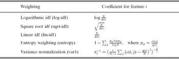
Global weighting. The global weighting schemes used in our experiments are summarized in Table 1. The most commonly used global weighting scheme, inverse of the document frequency (idf), assigns a high weight to terms that occur only in few documents and thus refer to very specific concepts. For term i, idf is the total number of documents N divided by the number of documents in which the word i occurs. In order to dampen the effect of the weight, usually logarithmic idf (log-idf) is applied (Jones Reference Jones1972), but different functions, such as square root (sqrt-idf) and identity (lin-idf), can also be applied. Entropy weighting, based on information theoretic principles, assigns the minimum weight to terms for which the distribution over documents is close to uniform and the maximum weight to terms that are concentrated in a few documents (Dumais Reference Dumais1991). Another method, more common for non-discrete data, is to normalize the variances of the features to one.

Table 1.

Five global weightings of words. N is the number of documents in a document collection, c(i, j) is the term frequency of word i in document j, g(i) = ∑_jc(i, j) is the global frequency of word i in the whole collection, d(i) = |{j:c(i, j)>0}| is the document frequency for word i, and σ_i ² is the sample variance for the term frequencies of word i

Length normalization. The length of the obtained vectors varies across the documents. The length depends on both the number of words present in each document and the applied local and global weightings. The similarities between the documents are often calculated with cosine similarity measure, which neglects the vector lengths (Salton and Buckley Reference Salton and Buckley1988). If some other distance measure is applied, the vectors can be explicitly normalized using, for example, L2 or L1 norms.

3.3 Evaluation methods for vector space models

The methods for measuring the quality of vector representations can be categorized as direct and indirect methods (Sahlgren Reference Sahlgren2006a). The direct methods compare the similarities in a vector space with external data, such as association norms or synonym tests, whereas the indirect methods measure the ability to solve a particular application task.

4.1 Mathematical foundation

Let p(s) be a probability distribution over documents s in one language. We assume that there exists a D_s-dimensional semantic space, denoted by _s, where the meanings of the documents can be encoded, and process _s that generates the instances of s from the instances z_s ∈ _s. Similarly, documents t in another language are generated from D_t-dimensional z_t ∈ _t using process _t. Furthermore, we assume that the semantic spaces for the two languages are subspaces in a global D_z-dimensional semantic space , and z_s and z_t are linearly dependent on instances of z. That is, given a meaning z ∈ , documents s and t are produced as

(12)

where and are rank D_s and rank D_t matrices, respectively. Assuming that _s and _t are independent processes, also s and t are independent when conditioned on z,

(13)

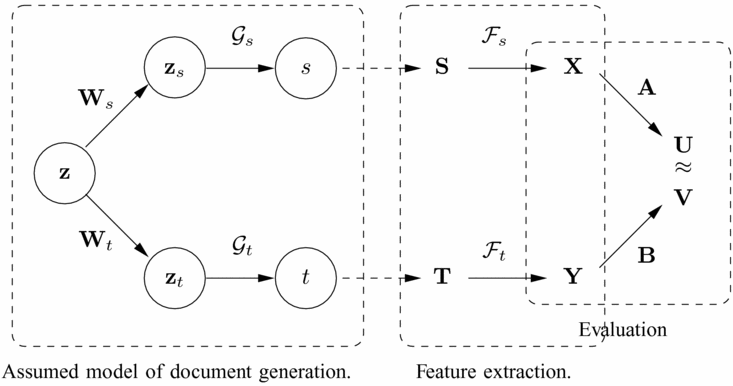
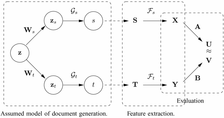
That is, the only thing that they have in common is their meaning, encoded in z. See the left part of Figure 1 for a graphical illustration of the assumed process of generation.

Fig. 1.

On the left: Assumed model for generation of documents s and t. Vector z in the language-independent semantic space is projected onto vectors z_s and z_t in the language-specific subspaces _s and _t. Processes _s and _t generate document pairs from the respective subspaces. On the right: The process of evaluating feature extraction method with CCA. The aligned document collections S and T are reduced to matrices X and Y of feature vectors using . Then X and Y are projected onto a common vector space using CCA.

Let us now consider a feature extraction method for the languages. Given two data sets of N documents S and T so that each s_i and t_i are samples from p(s | z_i) and p(t | z_i), transforms the documents into matrices X and Y:

(14)

If CCA is applied to X and Y, it will find projection matrices A and B that map X and Y to a common vector space as U = A^TX and V = B^TY, respectively, where . As explained in Section 2, CCA provides orthogonal U and V for which the row vectors have the highest correlations ρ_i = u_i v_i^T.

Using the assumed model of document generation with the original semantic document representations Z, we have

(15)

Intuitively, any feature from that does not originate from Z will decrease the correlations. In case the projections W_s and W_t do not lose any information (i.e., D_s = D_t = D_z and the matrices are invertible), we can show that when the feature extraction method is able to transform the documents back into the semantic spaces _s and _t, it provides the highest possible correlations: Inserting and to (15) results in

(16)

As the matrices W_s and W_t are invertible, we can simply set A^T = W_s^⊃1 and B^T = W_t ⁻¹, which gives UV^T = ZZ^T. Trivially, this leads to ρ_i = z_i z_i ^T/z_i z_i ^T = 1 for all i. Even if W_s and W_t are not square or full rank matrices, CCA gives the optimal solution for the corresponding eigenvalue problem. Thus, the evaluation, illustrated on the right part of Figure 1, should give insight on how well the tested methods extract features that correspond to the common meaning of the documents.

4.2 Evaluation setup

In the conventional evaluation setup, the learning algorithm – here a feature extraction method – is evaluated. One data set is needed for training the model (training set) and another for evaluating it (evaluation set). In our case, however, the evaluation method includes learning, i.e., calculating CCA. Learning the parameters of CCA either based on the training set of the feature extraction or the final evaluation set would enable over-fitting. Therefore, the evaluation set is divided into two distinct sets: an evaluation training set (evaltrain) and an evaluation test set (evaltest). The evaltrain set is used for training the parameters of CCA and the evaltest set as a test set for estimating the final correlations.Footnote ⁴

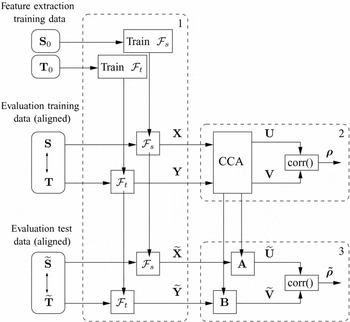
The requirement of the evaluation training set results in a three-stage evaluation setup as illustrated in Figure 2. At the first stage, the feature extraction method is trained for both the languages, using the monolingual training data sets S₀ and T₀. Both the evaltrain data (S, T) and the evaltest data are run through the feature extraction to obtain the aligned sets (X, Y) and .

Fig. 2.

Diagram of the evaluation setup. (1) The feature extraction method is trained on monolingual corpora and then applied to transform the evaluation data sets into vectorial form. (2) CCA is trained on the evaluation training data to find the canonical variates U and V and the respective projection matrices A and B. (3) The evaluation test data are then projected into the same space, and finally the test set correlations are computed.

At the second stage, the evaluation training set is used to calculate CCA as described in Section 2, resulting in the projection matrices A and B, the projected data sets U and V, and the correlations ρ = [ρ₁, . . ., ρ_D]. As a regularization, we add a small positive value ε proportional to the variances of X and Y to the diagonals of the respective covariance matrices C_xx and C_yy:

(17)

where S_x is a diagonal matrix with S _x(ii) = σ_xi², S_y is a diagonal matrix with S _y(ii) = σ_yi², and 0 < ε ≪ 1.

At the third stage we estimate how the learned features and the CCA projections together generalize to new data. Especially if the number of samples in the evaltrain set is low, or the dimensionalities of X and Y are high, the sample estimates of the covariance matrices are not robust. This leads to overlearning of the projection matrices A and B, regardless of the regularization. To find out how the learned projections can generalize outside the evaltrain set, we use them to project the evaltest set into the same common space, and calculate correlations for the resulting matrices. Assuming that and are centered, the test set correlations are calculated as follows:

(18)

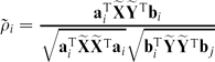
The vector of the test set correlations, , is used to obtain final score for the feature extraction method. The evaluation measures are discussed in the next subsection.

The covariance matrices C_xx, C_yy, and C_xy, which are needed in computing the canonical correlations, are non-sparse and thus the memory usage is of magnitude O(D_x ² + D_y ² + D_xD_y). In consequence, we need to keep the dimensionalities D_x and D_y low. It is convenient, but not necessary, to use representations that have the same dimensionality D for both languages. By performing the evaluation for a range of values for D, one may need to find the optimal dimensionality for the evaluated feature extraction method given the evaluation measure.

4.3 Evaluation measures

Learning the optimal projections with CCA and using them on the evaltest set gives us the correlation estimates . To make the evaluation more straightforward, we prefer to have a single value that measures the quality of a representation.

In the simplest case, we want to compare two vector representations having the same number of features returned by two feature extraction methods. Since the task is not to find a subset of the features, we do not consider only the largest correlation or the sum of few largest correlations. Instead, an intuitive measure is the sum over all the correlations:

(19)

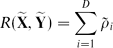
For perfectly correlated sets, R = D, and for uncorrelated sets, R = 0.

Canonical correlation analysis restricts the learned evaltrain correlations to be positive. However, the correlations from the evaltest set can also be negative due to random variation between the evaltrain and evaltest sets. It is justifiable that negative correlation coefficients decrease the score: such a coefficient for the test set indicate that CCA has learned something that does not generalize outside the evaltrain set. Moreover, forcing to be positive, for example, by taking the absolute value, would introduce a bias to its expected value.

Theoretically, MI would be a natural choice for an evaluation measure. However, as a general measure of dependence, MI can be inferred from the correlations only when the data are normally distributed. Still, even when we know that the data do not follow a Gaussian distribution, we can use (8) for MI to obtain a ‘Gaussian–MI’ score G . For uncorrelated sets, G = 0. An evident difference to the sum of correlations is that the Gaussian–MI score will give more weight to the correlations that have absolute values close to one. In fact, already one that is exactly one will set the score to infinity. Because of the squared correlation coefficients, negative values increase the score. However, as high negative values are very improbable, the effect is small in practice.

If the evaluated feature extraction methods return different number of features, the comparison of the vector representations is not straightforward. A problem with both the correlation sum and the Gaussian–MI score is that the scores tend to increase with the number of dimensions. An option would be to consider, for instance, the average correlation R /D. While the average correlation would directly penalize for having uncorrelated features, we find it unintuitive that, for example, the result = [0.9, 0.8] (D = 2) would be worse than = [0.9] (D = 1), as the representation in the former case surely encodes more semantic information than in the latter. Moreover, even a dimension that has a very small positive correlation can be useful if it is weighted according to the strength of the correlation, as shown by Tripathi et al. (Reference Tripathi, Klami and Kaski2008). We compare representations with different number of dimensions, first using an artificial example in Section 4.4 and later when validating the evaluation results with two sentence matching tasks in Section 5.3.

4.4 Examples

We demonstrate the proposed evaluation method on two artificial data sets. The goal is to show the effects of noise and dimensionality on the two evaluation measures, i.e., the sum of correlations and the Gaussian–MI score. In addition, the examples justify the need for separate test data set in the evaluation setup.

Example 1: Examining the effect of noise. Here we show how noise affects the evaluation scores. Consider the following normally distributed data with additive noise:

(20)

(21)

(22)

(23)

(24)

If the proportion of noise α = 1, then x and y are independent and the expected values for the correlation sum and Gaussian–MI scores are zero. If there is no noise at all (α = 0), then x and y have a perfect linear dependence. Using our regularization with coefficient ε, this results in expected correlation coefficients 1/(1 + ε). Thus,

(25)

(26)

R approaches D and G approaches infinity as ε approaches zero.

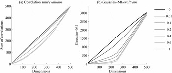
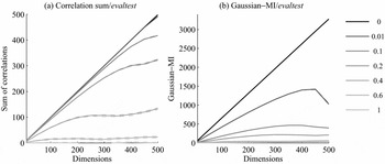
We used 500 samples of z as development data and 500 samples of z as test data. The test data was divided into fifty subsets. As we did not do feature extraction, training data were not needed. The dimensionality D was varied from 0 to 500 and the level of noise α from 0 to 1. In the evaluation, we applied regularization with ε = 10⁻⁶. We computed the sum of correlations and the Gaussian–MI scores for evaluation training and test data. In Figures 3 and 4 we use median (second quartile) and first and third quartiles to indicate the central tendency and variability of the results on the evaltest data.

Fig. 3.

Effect of different noise levels for evaluation training data: (a) Correlation sum R(X, Y), and (b) Gaussian–MI score G(X, Y). Lighter the tone of the curve, higher the noise level.

Fig. 4.

Effect of different noise levels for evaluation test data: (a) Correlation sum R , and (b) Gaussian–MI score G . Medians are drawn with solid lines. For consistency, also the first and third quartiles (dashed lines) are drawn, although these are very close to the median in these figures.

The correlations in the evaltrain data are high even with very noisy data (Figure 3). Especially if D is increased and the number of samples is fixed, the sample covariances become poor estimates for real covariances, and CCA overlearns. The use of the evaltest data for estimating the correlation clearly prevents the problem (Figure 4). As high correlations are obtained only when the learned projections generalize to new data, increasing D cannot improve the scores of the noisy data sets.

Example 2: Discovering the intrinsic dimensionality. Next, we consider data in which the intrinsic dimensionality is lower than those of the observed variables. The idea is to show that the evaluation method is able to detect the correct dimensionality given a suitable dimensionality reduction method. Assume that M-dimensional samples, x and y, are produced from a latent K-dimensional variable z, where K < M is the intrinsic dimensionality, as follows:

(27)

(28)

Again, we use normal distributions with zero mean and unit variance for z, n_x, and n_y. Let the weights in and be uniformly distributed between [−0.5 and 0.5]. Without noise, the maximal correlations for the D-dimensional features are R(x, y) ≈ min(D, K) × (1 − ε) and G(x, y) ≈ −min(D, K)/2 × ln(2ε) and thus remain constant for D > K.

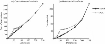
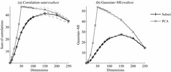
We compare PCA, which is a standard feature extraction method for the Gaussian data, and a trivial feature selection method that selects an arbitrary subset of features in x and y. We used 500 samples of z as a training set (i.e., for calculating the projections of PCA), another 500 samples as an evaluation training set, and once more 500 samples as an evaluation test set. Other parameters were α = 0.5, K = 50, and M = 250. Figure 5 shows the scores for the evaltrain data and Figure 6 for the evaltest data. The results show that PCA (gray line) performs considerably better than the baseline by just selecting a subset of variables (black line) when the dimensionality is near to the number of latent dimensions (50). Due to overlearning, the correlations for the evaltrain data continue to grow with dimensionality. For the evaltest data, however, they slowly start to decrease, thus clearly indicating the correct number of intrinsic dimensions.

Fig. 5.

Evaluation training set results for data with 50 intrinsic dimensions: (a) Correlation sum, and (b) Gaussian–MI score. In subset, a random subset of D dimensions of X and Y are selected. In PCA, the D first principal components are applied.

Fig. 6.

Evaluation test set results for data with 50 intrinsic dimensions: (a) Correlation sum, and (b) Gaussian–MI score. In subset, a random subset of D dimensions of X and Y are selected. In PCA, the D first principal components are applied. Medians are drawn with solid lines and the first and third quartiles with dashed lines.

5.1 Data sets

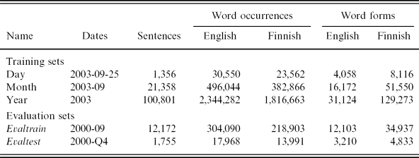
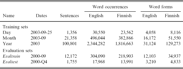
We used the Europarl corpus (version 2) that consists of the proceedings of the European Parliament meetings in eleven European languages (Koehn Reference Koehn2005). We applied standard preprocessing for the data that lowercased all letters and separated punctuation marks from words. The major parts of the experiments were performed with English–Finnish data, but Danish, German, and Swedish were also used. We extracted data sets of three different sizes for training feature extractions: one day of the corpus (2003-09-25), one month (2003-09), and one year (2003). As an evaluation training set, we applied the sentences that contained five to fifteen words in both the languages from the month 2000-09. As an evaluation test set, we used 1,755 sentences extracted by Koehn, Och and Marcu (Reference Koehn, Och and Marcu2003) from the last quarter of year 2000. The sentences contained five to fifteen words that were same for each language in the corpus. We divided the test set into ten parts and used the one-sided right-tailed Wilcoxon signed-rank test with significance level 0.05 to calculate statistical significances. The number of sentences, word occurrences, and different word forms are shown in Table 2. For practical reasons, we used the one-month training set for most of the experiments: It is small enough for fast calculation of different dimensionality reductions, but large enough to keep the out-of-vocabulary rates for the data sets used in the evaluation within reasonable limits.

Table 2.

The number of sentences, word occurrences, and word forms in the English–Finnish data sets

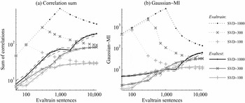
To find out whether the selected evaltrain data set was large enough for learning good correlation estimates, we run one feature extraction, SVD for plain cooccurrence counts, with different target dimensionalities for different sizes of the set. Figure 7 shows the estimated scores both from evaltrain and evaltest sets. The higher the dimensionality, the more data required before the estimates converge. Moreover, the gap between the evaltrain and evaltest results increases, showing that the high-dimensional features are less robust for the variation of the data. The full 12,000-sentence data can be considered large enough for reliable CCA results up to 1,000-dimensional representations.

Fig. 7.

Evaluation test and training set results for 100-, 300-, and 1,000-dimensional SVD features for different sizes of evaltrain set: (a) Correlation sum, and (b) Gaussian–MI score. Solid lines show the evaltest scores and dotted lines the evaltrain scores. The peaks in the evaltrain scores occur when the number of samples equals the number of dimensions.

5.2 Validation with known facts

A plausible evaluation method should be able to re-establish previously known facts concerning vector space models. We therefore consider five hypotheses from the literature and examine whether our evaluation method confirms them.

1. (1) Dimensionality reduction: SVD and PCA should perform better than other dimensionality reduction methods when the target dimensionality is relatively low (Deerwester et al. Reference Deerwester, Dumais, Landauer, Furnas and Harshman1990; Kaski Reference Kaski1998; Bingham and Mannila Reference Bingham and Mannila2001).

2. (2) Weighting: Among different global weighting schemes, entropy weighting and logarithmic idf should give the best improvements when using SVD (Dumais Reference Dumais1991; Nakov, Popova and Mateev Reference Nakov, Popova and Mateev2001).

3. (3) Amount of data: More training data should improve results whenever a reasonable dimensionality reduction method is applied. (Zelikovitz and Hirsh Reference Zelikovitz, Hirsh and Nebel2001; Yarowsky and Florian Reference Yarowsky and Florian2002).

4. (4) Phrases as features: Generally, it does not seem to help if observed phrases (e.g., 2-grams) from the training data are included as features (Lewis Reference Lewis1992; Scott and Matwin Reference Scott and Matwin1999; Caropreso, Matwin and Sebastiani Reference Caropreso, Matwin, Sebastiani and Chin2001; Sebastiani Reference Sebastiani2002; Koster and Seutter Reference Koster and Seutter2003; Coenen et al. Reference Coenen, Leng, Sanderson and Wang2007).

5. (5) Effect of language similarity: Due to morphological and syntactic similarities, closely related languages should have higher correlations than, for example, languages that belong to different language families (Besançon and Rajman Reference Besançon and Rajman2002; Chew and Abdelali Reference Chew and Abdelali2007; Sadeniemi et al. Reference Sadeniemi, Kettunen, Lindh-Knuutila and Honkela2008).

Except for the fourth experiment, in which bag-of-phrases are tested, we used the basic bag-of-words representations for the sentences. All the word forms, including punctuation marks, were collected to form the word–sentence matrix , where _ij is the number of times word i occurred in sentence j. Except for the first experiment, the matrix was weighted according to global and local weightings, and the dimensionality was reduced with SVD. We experimented with a range of dimensionalities D from 10 to 1300.

5.2.1 Dimensionality reduction

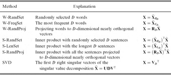
We compared seven dimensionality reduction methods that we summarize in Table 3. Three of them were based on the first-order information (see Section 3). We used two feature selection methods: taking a random subset of words (W-RandSet) and taking the words with the highest sentence frequency (W-FreqSet). We also tested random projection for the words (W-RandProj).

Table 3.

The evaluated dimensionality reduction methods. is the original data matrix and X is the reduced data matrix

As second-order dimensionality reduction, we used the following four methods. The first one is a naive approach, which selects a random subset of sentences (S-RandSet). The next approach is to select sentences that contain the highest number of word types, because intuitively they provide more information (S-LenSet). We also used random projection, where the random vectors are now sampled for each sentence rather than each word (S-RandProj). Finally, we tested SVD.

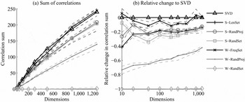
The left side of Figure 8 shows the correlation sum results. Its right side shows same results using relative differences to SVD and a logarithmic scale for dimensionality, making differences more clear. W-FreqSet and SVD clearly outperformed other methods. SVD was significantly better than W-FreqSet for all dimensionalities except for D = 10 (significantly worse), D = 900 (significantly worse), and D = 1, 300 (no statistically significant difference). S-RandProj was usually the best of the other second-order methods, but the difference to S-LenSet was statistically significant only for D ∈ {10, 20, 200, 300}.

Fig. 8.

Results for different dimension reduction methods: (a) Absolute sum of correlations. The dashed lines show the first and third quartiles for the results of each method. (b) Relative change compared to SVD. The reference (SVD) does not have quartile lines, because the relative differences were calculated separately for each subset and the deviation is thus included in the results of the compared methods.

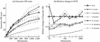
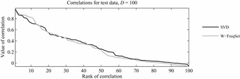
Figure 9 shows the results for the Gaussian–MI score. The results are similar to the sum of correlations except that W-FreqSet is closer to SVD and even outperforms it at D = 100. To illustrate the reason for the conflicting results, Figure 10 gives a closer look at the distribution of test correlations for W-FreqSet and SVD. While SVD has on average higher correlations (as indicated by the higher sum), the first few values ranked from 1 to 13 are higher for W-FreqSet. Since the function −ln(1 − ρ_i ²) gives much emphasis to values close to one and little to those near to zero, this explains why W-FreqSet has better Gaussian–MI score than SVD. In the extreme case if there was a single correlation very close to one and the rest were zeros, the Gaussian–MI score would still be high. We used only correlation sum for the remaining experiments to avoid this problem.

Fig. 9.

Results for the different dimension reduction methods: (a) Absolute Gaussian–MI scores, and (b) relative change compared to SVD. The dashed lines show the first and third quartiles for the results.

Fig. 10.

Individual test correlations for SVD and W-FreqSet dimensionality reductions for D = 100. Values of the correlations are shown in descending order.

To sum up, our evaluation prefers SVD in lower dimensionalities. This is in agreement with previous studies (Deerwester et al. Reference Deerwester, Dumais, Landauer, Furnas and Harshman1990). Moreover, the order of other dimensionality reduction methods was intuitive.

5.2.2 Weighting and normalization

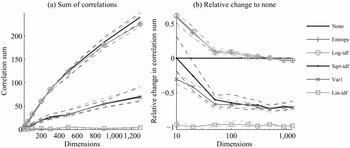
In the previous experiment, no feature weighting was applied. In our second experiment, we use SVD for dimensionality reduction and compare the global term weightings described in Table 1. Figure 11 shows (a) the sum of correlations for the weighting methods, and (b) the relative difference to the baseline without weighting.

Fig. 11.

Results for different global weightings: (a) Absolute sum of correlations, and (b) relative change compared to no weighting. The dashed lines show the first and third quartiles for the results of each method.

Again, the results are in line with the previous findings (Dumais Reference Dumais1991; Nakov et al. Reference Nakov, Popova and Mateev2001). The logarithmic idf and entropy weightings improved the baseline results significantly for the lower dimensionalities (D < 200). Up to D = 500, there was no significant difference, and for D ≥ 1,000, the weighting decreases the result. We did not find significant differences between logarithmic idf and entropy weightings as found by Dumais (Reference Dumais1991). The rest of the weightings gave scores significantly below the baseline. Linear idf was always the worst.

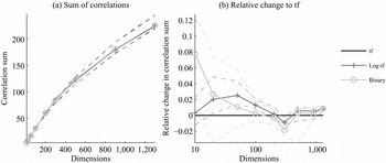
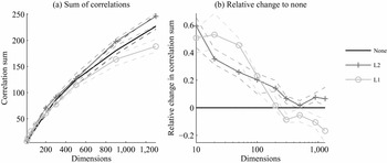
We also tested different local weightings (no, binary, and logarithmic weight) for the term frequencies and length normalizations (no, L1, and L2 normalization) with entropy weighting and SVD. The logarithmic term frequency outperformed plain term frequency significantly for some dimensionalities (D ∈ {20, 50, 100, 1300}) and was never worse, as shown in Figure 12. Using binary values was better than logarithmic term frequency (and term frequency) only for D = 10. With log-term frequency and entropy weighting, L2 normalization was significantly better than no length normalization except for D = 500, where the difference was not significant (Figure 13). L1 was significantly better than L2 for some low dimensionalities (D ∈ {20, 50}). However, it was even worse than no normalization for high dimensionalities (D ≥ 300). Thus, the most robust setting for SVD seems to be the entropy weighting as the global weighting, logarithmic term frequency as the local weighting, and L2 normalization of the lengths. We applied this for the rest of the experiments.

Fig. 12.

Results for different local weightings: (a) Absolute sum of correlations, and (b) relative change compared to no weighting. The dashed lines show the first and third quartiles for the results of each method.

Fig. 13.

Results for different length normalizations: (a) Absolute sum of correlations, and (b) relative change compared to no normalization. The dashed lines show the first and third quartiles for the results of each method.

5.2.3 Amount of data

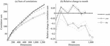
As a third experiment, we studied the effect of the size of the training set for feature extraction methods. Figure 14 shows the absolute correlation sums and the relative difference to the results with the one-month data set. The one-year data set gave significantly better correlation sums than the one-month data set for D ∈ {20, 100, 200} and significantly worse results only for D = 10. The one-day data set gave significantly worse results than the larger sets except for D = 20, where the difference to the one-month set was not significant. Thus, our evaluation method shows that more training data improve results, which conforms with the findings of, for instance, Zelikovitz and Hirsh (Reference Zelikovitz, Hirsh and Nebel2001) and Yarowsky and Florian (Reference Yarowsky and Florian2002). The finding is especially pronounced in higher dimensionalities, which has been already noticed, for example, by Bradford (Reference Bradford2008).

Fig. 14.

Results for different sizes of training data for SVD: (a) Absolute sum of correlations, and (b) relative change compared to the one-month data set. For the year data set, we used dimensionality up to 500 only due to high computational requirements.

5.2.4 Phrases as features

Intuitively, the bag-of-words representation may not always be the optimal representation for sentences, because it discards the information on the word order. A simple extension is to use sequences of multiple words, n-grams, as additional features. However, previous work on the bag-of-phrases models shows that including n-grams does not improve the results in tasks, such as text categorization, unless the n-grams are selected carefully (Lewis Reference Lewis1992; Scott and Matwin Reference Scott and Matwin1999; Caropreso et al. Reference Caropreso, Matwin, Sebastiani and Chin2001; Sebastiani Reference Sebastiani2002; Koster and Seutter Reference Koster and Seutter2003; Coenen et al. Reference Coenen, Leng, Sanderson and Wang2007).

We tested the evaluation for representations in which the n-grams up to a maximum length N that had been observed in the training data at least twice were included as separate features in addition to all the observed word forms. Table 4 shows the number of features in the English–Finnish data for n = 2 and n = 5. Similar to the bag-of-words baseline, we applied SVD, log-term frequency and entropy weightings, and L2 normalization to get final representations.

Table 4.

The amount of n-gram types in the English and Finnish training data. For n > 1, n-grams occurring only once are discarded

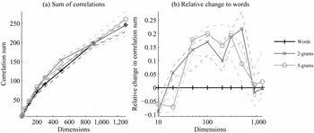
Figure 15 shows (a) the correlation sums for bag-of-words and bag-of-phrases with n = 2 and n = 5, and (b) the relative changes to bag-of-words with logarithmic scale for dimensionality. Bag-of-words outperformed bag-of-phrases only for very low dimensionalities (D = 10 for 2-grams and D ∈ {10, 20} for 5-grams). For D ≥ 1,000, there was no statistically significant differences. Otherwise, both 2-grams and 5-grams provided statistically significant improvements for correlation sum. The order of the two was not clear: sometimes 2-grams were better (D ∈ {20, 500}), sometimes 5-grams (D ∈ {50, 200}), and sometimes there was no significant difference.

Fig. 15.

Correlation sums for test data using n-gram features of different lengths: (a) Absolute sum of correlations, and (b) relative change compared to words.

Our method for selecting the phrases was very simple. Thus, the results are in contrast with the previous studies, in which only sophisticated selection methods, if any, have provided improvements. One reason may be that the word order information is more important for the meaning of single sentences than for longer documents. This would require further study with a different type of data set.

5.2.5

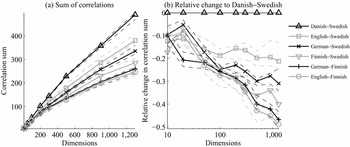
A reasonable hypothesis is that closely related languages will be more correlated than distant languages Besançon and Rajman Reference Besançon and Rajman2002; Chew and Abdelali Reference Chew and Abdelali2007; Sadeniemi et al. Reference Sadeniemi, Kettunen, Lindh-Knuutila and Honkela2008). The results for the test data using similar bag-of-words (entropy weighting, L2 normalization, and dimensionality reduction with SVD) representations for six language pairs are shown in Figure 16. For the highest dimensionalities (D ≥ 500), the order of the scores follow the closeness of the languages: (1) Among the language pairs, the most correlated were Danish and Swedish, two closely related North Germanic languages. (2) The languages in the three least correlated pairs belonged to different language families: one of the languages was always Finnish, which is an Uralic language, and the other was English, German, or Swedish, which are all Indo-European and Germanic languages. (3) Finnish was more correlated with Swedish than any other of the Germanic languages, which may be due to the close cultural proximity of speakers of the two languages.

Fig. 16.

Correlation sums for test data with different language pairs: (a) Absolute sum of correlations, and (b) relative change compared to Danish–Swedish.

5.3 Validation with sentence matching tasks

An indirect way to evaluate the quality of vector representations for bilingual corpus is to check how well the sentences that are translations of each other can be matched based on a vector space model. We compared our proposed direct approach to an indirect approach of using sentence matching for evaluation. The idea is to show that any vector representation that performs well on our evaluation approach also performs well on the sentence matching task.

We considered the task of matching in two different settings. In the first setting, we used the projected sets U and V to find the closest sentence in English for a sentence in Finnish and checked if it was a correct translation. We also searched for a match in the other direction and took the average of two accuracies. This task is similar to the nearest translation test done by Besançon and Rajman (Reference Besançon and Rajman2002). In the second setting, we found one-to-one alignment of sentences using the Hungarian algorithm (Kuhn Reference Kuhn1955), weighting the dimensions of canonical variates with corresponding evaltrain correlations in a similar manner as done by Tripathi, Klami and Virpioja (Reference Tripathi, Klami and Virpioja2010).

We first validated the evaluation scores for 100-dimensional representations obtained from the previous experiments: the different dimensionality reductions without weighting, weighted SVD for the one-day, the one-month, and the one-year data sets, and the two bag-of-phrases representations. The test data were divided into 100 subsets of seventeen to eighteen sentences, and both the correlations and matching accuracies were calculated for each set.

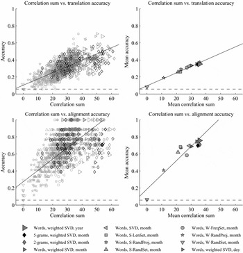
Figure 17 shows scatter plots of accuracy in the nearest translation test (top) and the alignment task (bottom) versus the correlation sum. For the translation task, Spearman's rank correlation coefficient between the correlation sums and accuracies was 0.776 over the subsets and 1.0 over the means. For the alignment task, correlation was 0.633 over the subsets and 0.888 over the means. We also considered how the two related tasks, translation and alignment, could predict each other as indirect evaluations. That is, we compared the translation and alignment accuracy based on the two tasks. The correlation coefficient was 0.627 over the subsets and 0.888 over the means. Hence, indirect evaluations based on two very similar tasks could not predict each other's performance any better than the proposed direct evaluation. This shows that our evaluation method is at least as good as evaluation methods based on a sentence matching task.

Fig. 17.

Translation (top) and alignment (bottom) accuracy versus correlation sum over the test data subsets. The left side shows individual values for each subset and the right side shows the mean values for the different representations. The solid lines show the best linear least squares fit of data points. The dashed horizontal line shows the average baseline result of a random choice.

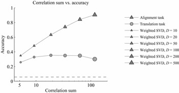
Finally, we calculated the results for representations of different dimensionalities. Figure 18 compares the correlation sums and accuracies of weighted SVD with D ∈ {10, 20, 50, 100, 200, 500} using the translation and alignment tasks. The alignment accuracy grows logarithmically with respect to the correlation sum, indicating that the components that are correlated only slightly are useful if weighted accordingly. In contrast, the translation accuracy starts to decrease already after D = 50. Thus, there seems to be no way to score the representations of different dimensionalities so that the scores would agree with all application evaluations.

Fig. 18.

Translation and alignment accuracies versus correlation sum. The points are mean values for 10, 20, 50, 100, 200, and 500 dimensional SVD representations.

5.4 Validation with manual evaluation of word translations

Our evaluation method based on CCA has an advantage that the canonical variates are interpretable: For a given canonical variate, we can find which original features, for example, words, contribute to it by calculating canonical factor loadings (6). As an example from SVD trained with one-month data, there is a variate that strongly correlates with English words vote, place, take, tomorrow, and noon and Finnish words äänestys (vote in English), toimitetaan (takes place), klo (at [time]), huomenna (tomorrow), and 12.00 (noon). While these are not direct translations, it is easy to see that they come from same sentences in each language. This is a desirable behavior due to the sentence-aligned corpus. We use the correctness of such word translations to compare different representations. A method performing well according to the evaluation method should also provide good translations.

We compared the five most positively and negatively correlated original features for both the languages to see if they refer to the same meaning. For the two sets of words corresponding to a given canonical variate, we counted the number of correct translations. Translations were checked in both the directions and the sum of the correct translations was used in the evaluation. Thus, the maximum score for one canonical variate is (5 + 5) × 2 = 20. We computed the scores for each canonical variate and used the sum as an evaluation measure.

We used the one-month data with four different dimensionality reduction methods: SVD, S-LenSet, W-FreqSet, and W-RandProj with term frequency weighting and no normalization. In addition, two more settings were tested for SVD: entropy weighting together with L2 normalization for both the one-month and one-year data. The dimensionality was reduced to 100, which was then the number of canonical variates to evaluate.

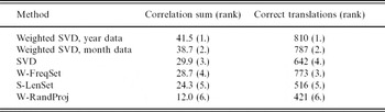
Table 5 shows the correlation sum and the number of correct translations found for different vector representations. It can be clearly seen that the representations with high correlation sum also provided large number of correct translation pairs. Correlation between the two scores was 0.9772. The only difference in the ranks is for SVD and W-FreqSet. They reached almost the same correlation sum, but the evaluated factor loadings for W-FreqSet had more correct translations.

Table 5.

Evaluation results of different dimensionality reduction methods and different settings for SVD using the correlation sum and the number of correct translations