1 Introduction
The distributional similarity methods have proven to be a valuable tool for the induction of semantic similarity. The aggregate of a word's contexts generally provides enough information to compute its meaning, viz. its semantic similarity or relatedness to other words.
Until now, most algorithms use two-way co-occurrence data to compute the meaning of words. A word's meaning might, for example, be computed by looking at
• the various documents that the word appears in (words × documents);
• a bag of words context window around the word (words × context words);
• the dependency relations that the word appears with (words × dependency relations).
The extracted data – representing the co-occurrence frequencies of two different entities – is encoded in a matrix. The co-occurrence frequencies, however, need not be pairwise. One can easily imagine situations where it is desirable to investigate the co-occurrence frequencies of three modes and beyond. In an information retrieval context, one such situation might be the investigation of words × documents × authors. In a Natural Language Processing (nlp) context, one might want to investigate words × dependency relations × bag of word context words, or verbs × subjects × direct objects.
Note that it is not possible to investigate the three-way co-occurrences in a matrix representation form. It is possible to capture the co-occurrence frequencies of a verb with its subjects and its direct objects, but one cannot capture the co-occurrence frequencies of the verb appearing with the subject and the direct object at the same time. When the actual three-way co-occurrence data is ‘matricized’, valuable information is thrown away. To be able to capture the mutual dependencies among the three modes, we will make use of a generalized tensor representation. The two-way co-occurrence models (such as latent semantic analysis) have often been augmented with some form of dimensionality reduction in order to counter noise and overcome data sparseness. We will also make use of dimensionality reduction algorithms appropriate for tensor representations.
In this paper, we will focus on the benefit of three-way methods in the framework of selectional preference induction. Selectional preferences are a useful and versatile resource for a number of applications, such as syntactic disambiguation (Hindle and Rooth Reference Hindle and Rooth1993), semantic role labeling (Gildea and Jurafsky Reference Gildea and Jurafsky2002), and word sense disambiguation (McCarthy and Carroll Reference McCarthy and Carroll2003). The selectional preference of a verb can be defined as the semantic restrictions that the verb imposes on its arguments (and thus the preference it has for particular semantic classes).Footnote 1 A verb like drink, for example, typically prefers animate subjects and drinkable objects. A selectional preference model keeps track of these semantic classes that verbs prefer for their argument slots.
The standard selectional preference models take the form of a mapping σ: (v, r, c) ↦ a, that maps each selectional tuple (v, r, c) to a real number a, representing the degree of preference of a verb v for a class c with respect to role r (Light and Greiff Reference Light and Greiff2002). Keeping track of single relationships, however, is not enough to build a sufficiently rich model of selectional preferences. Compare the following sentences:
(1) The skyscraper is playing coffee.
(2) The turntable is playing the piano.
The first sentence is a clear violation of the selectional preferences of play, both for its subject and object slot: a skyscraper doesn't play, nor is coffee something that can be played. The standard selectional preference models are able to capture this violation, because both (play, su, skyscraper) and (play, obj, coffee) will not be deemed very plausible by these models. The second sentence, however, is more complicated. The sentence still constitutes a violation of the selectional preferences (turntables are not able to play piano's), but the violation is due to the ambiguity of the verb play, and the individual preferences (play, su, turntable) and (play, obj, piano) are perfectly possible. The standard models, therefore, will not be able to capture this violation. By keeping track of the three-way co-occurrence data, we hope to build a richer model of selectional preferences that does justice to preference violations like the one in sentence 1. Moreover, by using a factorization technique suitable for three-way co-occurrences, we hope to build a three-way selectional preference model that is able to generalize to unseen data.
The paper is organized as follows. In the next section, we give an overview of previous work related to this paper; we discuss previous approaches to selectional preferences and verb clustering, and give an overview of factorization algorithms that have been used for language processing. Section 3 discusses the methodology of three-way factorizations, including an overview of tensors and their algebra. In Section 4, we describe the application of the three-way factorization model for the induction of selectional preferences, and illustrate the kind of data the model is able to capture with some examples. Section 5, then, presents a quantitative evaluation of the model using a pseudo-disambiguation task, and compares the results to other approaches. Section 6, finally, wraps up with some conclusions and pointers for future work.
2 Previous work
2.1 Selectional preferences and verb clustering
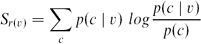
Selectional preferences have been a popular research subject in the nlp community. Research on the subject dates back to the early nineties, with early approaches given in Basili, Pazienza and Velardi (Reference Basili, Pazienza and Velardi1992) and Grishman and Sterling (Reference Grishman and Sterling1992). One of the most influential approaches to the automatic induction of selectional preferences from corpora is the work of Resnik (Reference Resnik1993, Reference Resnik1996). Resnik generalizes among nouns by using WordNet noun synsets as semantic classes. He then calculates the selectional preference strength Sr(v) of a specific verb v in a particular relation r by computing the Kullback–Leibler divergence between the class distribution of the verb p(c | v) and the aggregate class distribution p(c):
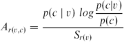
The selectional association Ar(v,c) is then the contribution of a particular semantic class c to the verb's preference strength:
The model's generalization relies entirely on WordNet; there is no generalization among the verbs. Other notable approaches using WordNet for selectional preference induction are given by Abe and Li (Reference Abe and Li1996) and Clark and Weir (Reference Clark and Weir2001).
The research in this paper is related to previous work on clustering. Pereira, Tishby and Lee (1993) use an information-theoretic-based clustering approach, clustering nouns according to their distribution as direct objects among verbs, conditioned on a set of latent semantic classes

Their model is an asymmetric, one-sided clustering model: only the direct objects are clustered, there is no clustering among the verbs.
Rooth et al. (Reference Rooth, Riezler, Prescher, Carroll and Beil1999) use an Expectation-Maximization (em)-based clustering technique to induce a clustering based on the co-occurrence frequencies of verbs with their subjects and direct objects. Their clustering model is the same as the one used by Pereira et al. (Reference Pereira, Tishby and Lee1993), but they have embedded the model in a formal em-clustering framework. Rooth et al.'s (Reference Rooth, Riezler, Prescher, Carroll and Beil1999) clustering is two-sided: the verbs as well as the subjects/direct objects are clustered. We will use a similar model for evaluation purposes.
Recent approaches using distributional similarity methods for the induction of selectional preferences are the ones given by Bhagat, Pantel and Hovy (Reference Bhagat, Pantel and Hovy2007), Basili et al. (Reference Basili, De Cao, Marocco and Pennacchiotti2007) and Erk (Reference Erk2007). Erk (Reference Erk2007) uses corpus-based similarity measures for the induction of selectional preferences. The selectional preference Srv for an argument slot r of a particular verb v and a possible headword w 0 is computed as the weighted sum of similarities between w 0 and the headwords seen as argument fillers for the verb (Seen(rv)); wtrv is an appropriate weighting function

Both Basili et al. (Reference Basili, De Cao, Marocco and Pennacchiotti2007) and Bhagat et al. (Reference Bhagat, Pantel and Hovy2007) investigate the induction of selectional preferences in the context of textual entailment tasks.
This research differs from the above-mentioned approaches by its use of multi-way data: where the above approaches limit themselves to two-way co-occurrences, this research will extend the notion of selectional preferences for multi-way co-occurrences.
2.2 Factorization methods
2.2.1 Two-way factorizations
A number of factorization methods have been employed in natural language processing applications, mainly for the computation of semantic similarity. One of the best-known methods using a two-way factorization is latent semantic analysis (lsa) (Landauer and Dumais Reference Landauer and Dumais1997; Landauer, Foltz and Laham Reference Landauer, Foltz and Laham1998). Latent semantic analysis models the meaning of words and documents by projecting them into a vector space of reduced dimensionality; the reduced vector space is built up by applying the singular value decomposition (svd) – a well-known linear algebraic method – to a term-by-document frequency matrix. The resulting lower dimensional matrix is the best possible fit in a least squares sense. By enforcing a lower number of dimensions, the algorithm is forced to make generalizations over the simple frequency data. The Co-occurring terms are mapped to the same dimensions; terms that do not co-occur are mapped to different dimensions. lsa allegedly finds ‘latent semantic dimensions’, according to which nouns and documents can be represented more efficiently.
While rooted in linear algebra, singular value decomposition has proven to be a useful tool in statistical applications. It is closely akin to statistical methods, such as principal components analysis, and has been used as a versatile dimensionality reduction technique in different scientific fields, such as image recognition, information retrieval and signal processing (Deprettere Reference Deprettere1988). svd stems from a well-known theorem in linear algebra: A rectangular matrix can be decomposed into three other matrices of specific forms, so that the product of these three matrices is equal to the original matrix:

where z = min(m, n).
The singular value decomposition can be interpreted as a method that rotates the axes of the n-dimensional space in such a way that the largest variation is captured by the leading dimensions. The diagonal matrix Σ contains the singular values sorted in descending order. Each singular value represents the amount of variance that is captured by a particular dimension. The left-singular and right-singular vectors linked to the highest singular value represent the most important dimension in the data (i.e. the dimension that explains the most variance of the matrix); the singular vectors linked to the second highest value represent the second most important dimension (orthogonal to the first one) and so on. Typically, one uses only the first k ≪ z dimensions, stripping off the remaining singular values and singular vectors. If one or more of the least significant singular values are omitted, then the reconstructed matrix will be the best possible least-squares approximation of the original matrix in the lower dimensional space. Intuitively, svd is able to transform the original matrix – with an abundance of overlapping dimensions – into a new, many times smaller matrix that is able to describe the data in terms of its principal components. Due to this dimension reduction, a more succinct and more general representation of the data is obtained. Redundancy is filtered out, and data sparseness is reduced.
Latent semantic analysis has been criticized for a number of reasons, one of them being the fact that the factorization contains negative numbers. It is not clear what negativity on a semantic scale should designate. Subsequent methods, such as probabilistic latent semantic analysis (Hofmann Reference Hofmann1999) and non-negative matrix factorization (Lee and Seung Reference Lee and Seung2000), remedy these problems, and indeed get much more clear-cut semantic dimensions. Below, we discuss the latter method in more detail.
The non-negative matrix factorization (nmf) is a method that factorizes a matrix V into two other matrices, W and H:

Typically, r is much smaller than n, m so that both instances and features are expressed in terms of a few components. The nmf enforces the constraint that all three matrices must be non-negative, so that all elements must be greater than or equal to zero. The factorization is carried out by minimizing an objective function, typically the least squares error (7):

Practically, the factorization can be efficiently computed through the iterative application of multiplicative update rules. The set of update rules that minimize the least square errors are given in (8) and (9):
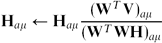
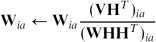
Matrices W and H are randomly initialized, and the update rules are iteratively applied – alternating between them. In each iteration, the matrices W and H are suitably normalized, so that the rows of the matrices sum to 1. The algorithm stops after a fixed number of iterations, or according to some stopping criterion (the change of the objective function drops below a certain threshold). The update rules are guaranteed to converge to a local optimum.
We will use both singular value decomposition and non-negative matrix factorization for reasons of comparison in our evaluation framework.
2.2.2 Three-way factorizations
To be able to cope with three-way data, several algorithms have been developed as multilinear generalizations of the svd. In statistics, the three-way component analysis has been extensively investigated (for an overview, see Kiers and van Mechelen Reference Kiers and van Mechelen2001). The two most popular methods are the parallel factor analysis (parafac) (Carroll and Chang Reference Carroll and Chang1970; Harshman Reference Harshman1970) and the Tucker decomposition (Tucker Reference Tucker1966). Three-way factorizations have been applied in various domains, such as psychometry and image recognition (Vasilescu and Terzopoulos Reference Vasilescu and Terzopoulos2002). In information retrieval, three-way factorizations have been applied to the problem of link analysis (Kolda and Bader Reference Kolda and Bader2006).
One last important method dealing with multi-way data is the non-negative tensor factorization (ntf) (Shashua and Hazan Reference Shashua and Hazan2005). ntf is a generalization of non-negative matrix factorization, and can be considered an extension of the parafac model with the constraint of non-negativity (cfr. infra).
One of the few papers that has investigated the application of tensor factorization for nlp is Turney (Reference Turney2007), in which a three-mode tensor is used to compute the semantic similarity of words. The method achieves 83.75 percent accuracy on the toefl synonym questions.
3 Methodology
3.1 Three-way data
The distributional similarity methods usually treat language data as two-way occurrences, represented in the form of a matrix. The matrix representation is perfectly suited for the representation of two-way co-occurrence phenomena; it allows for the application of algebraic and statistical methods, which in turn allow for the induction of semantic generalizations. The reduction of language to two-way co-occurrence frequencies, however, is a vast oversimplification. Language is a complex system of interrelated words, driven a.o. by grammar rules and subcategorization frames. By keeping track of multi-way co-occurrences, we can attempt to do some more justice to this complexity (although the framework represented here remains a major simplification). Compare the following sentences:
(3)

(4)

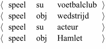
The dependency relations (subject–verb and verb–object) for examples 3.1 and 3.1 are given in Figure 1.
Extracted dependency relations.
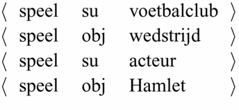
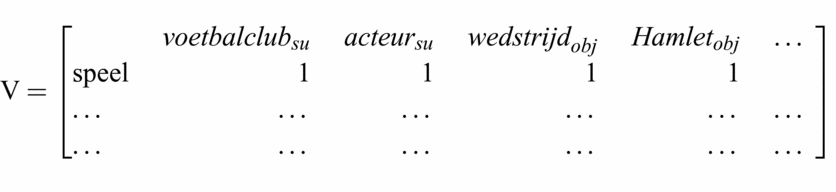
Say, we now want to investigate the semantics of Dutch verbs (like spelen ‘to play’). In our standard two-way framework, we would then take the verbs to be one mode, and combine the syntactic dependencies that the verbs appear with (subjects and direct objects in this case) together in the other mode, yielding a matrix like the one in Figure 2.
Two-way co-occurrence matrix.
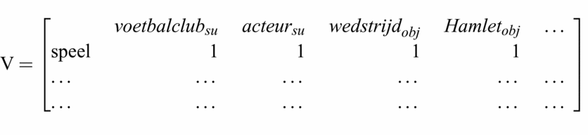
This is a genuine and appropriate way of investigating a verb's semantics, but we do lose some more complex and interesting relations between a verb and its objects. By capturing a verb's co-occurrences in a matrix form, we are able to investigate its co-occurrence with particular subjects and direct objects separately, but we are not able to investigate a verb's co-occurrence with subjects and direct objects at the same time: we lose the three-way relationship that exists between verb, subject and direct object.
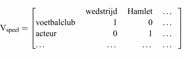
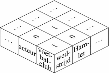
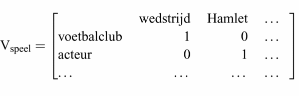
It is possible, however, to capture in a matrix the relationship between subjects and direct objects for one particular verb. For the above examples with spelen, this yields the matrix given in Figure 3. The rows of the matrix represent the subjects, and the columns represent the direct objects. A graphical representation of this matrix is given in Figure 4.
Two-way co-occurrence matrix of subjects and direct objects for the verb spelen ‘to play’.
Graphical representation of the co-occurrence matrix for the verb spelen ‘to play’.

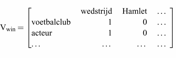
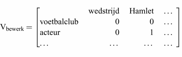
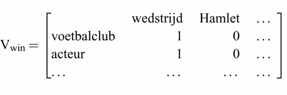
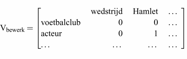
We can now construct similar matrices for each verb that we want to investigate. Say, we want two include two more verbs, winnen ‘to win’, and bewerken ‘to adapt’. The matrices for these verbs are given in Figures 5 and 6. Note that the two matrices Vwin and Vbewerk contain the same instances and features (subjects and direct objects) in their rows and columns as the first matrix Vspeel.
Two-way co-occurrence matrix of subjects and direct objects for the verb winnen ‘to win’.
Two-way co-occurrence matrix of subjects and direct objects for the verb bewerken ‘to adapt’.
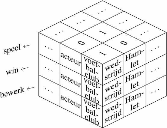
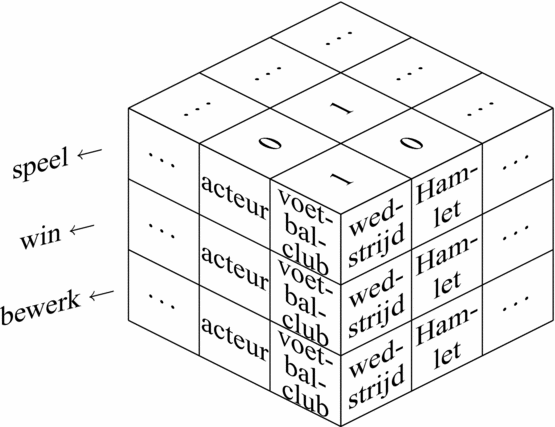
As a last step, we can now stack the three matrices together, which yields a three-dimensional cube like the one shown in Figure 7.
Graphical representation tensor.
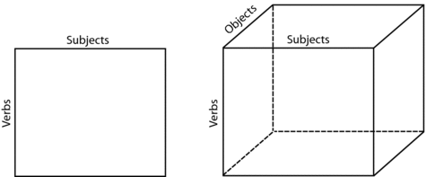
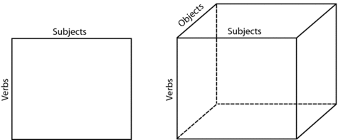
It would be clear by now that we are leaving the familiar domain of two-dimensional matrices. As we have noted before, a matrix is not a suitable form for the representation of multi-way data. For co-occurrence data beyond two modes, we need a more general representation. The generalization of a matrix is called a tensor. A tensor is able to encode co-occurrence data of any n modes. Figure 8 shows a graphical comparison of a matrix and a tensor with three modes – although a tensor can easily be generalized to more than three modes.Footnote 2
Matrix representation versus tensor representation.
We are now leaving the familiar domain of two-dimensional matrix algebra, and enter the realm of higher dimensional tensor algebra. Tensor algebra involves some novel mathematical machinery. The next section provides a succinct introduction to tensor algebra.
3.2 Tensor algebra
In this overview of tensor algebra, we will review some conceptual and notational preliminaries based on Kiers (Reference Kiers2000) and Kolda and Bader (Reference Kolda and Bader2009), and focus on some vital tensor operations required for the tensor-based factorizations explained in the next section.
The order of a tensor is its number of ‘dimensions’.Footnote 3 Vectors (tensors of order one) are denoted by boldface lowercase letters (x). Matrices (tensors of order two) are denoted by boldface capital letters (X). Higher order tensors (order three or higher) are denoted by boldface calligraphic letters ( ). Scalars are denoted by lowercase letters (x).
The ith entry of a vector x is written as xi, element ij of a matrix X is written as xij and element (i, j, k) of a third-order tensor is written as xijk. Indices range from 1 to D, so that i = 1, . . ., D. The nth element in a sequence is written as a superscript in parentheses, so A(n) denotes the nth matrix in a sequence.
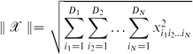
The norm of a tensor ∈ ℝD 1 × D 2 × D 3 – analogous to the Frobenius norm for matrices – is the square root of the sum of squares of all its elements (10):
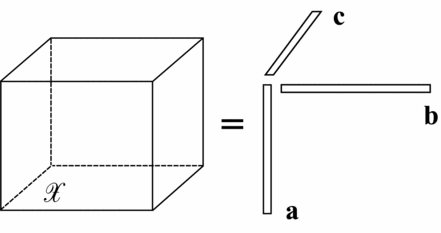
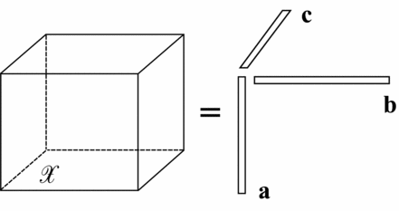
An N-order tensor ∈ ℝD 1 × D 2 × . . . × DN) is of rank one if it can be written as the outer product of N vectors:

The small circle (○) denotes the outer product and is calculated by multiplying for each element of the tensor the corresponding vector elements:

A third-order rank one tensor is given in Figure 9.
A third-order rank one tensor, which can be written as the outer product of three vectors.
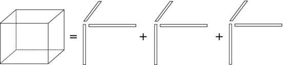
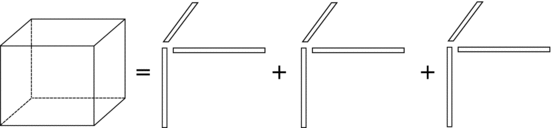
Finally, the rank of a tensor is defined as the smallest number of rank one tensors whose sum is equal to . Figure 10 shows a tensor that can be generated with the sum of three rank one tensors (the sum of three outer products). Therefore, rank()= 3).
A third-order tensor of rank three, which can be written as the sum of three outer products.
3.3 Multi-way factorization algorithms
In the next sections, we will look in some more detail at two different (but related) multi-way factorization algorithms: parallel factor analysis and non-negative tensor factorization. An extensive overview of multi-way data analysis is given in Acar and Yener (Reference Acar and Yener2009) and Kolda and Bader (Reference Kolda and Bader2009).
3.3.1 Parallel factor analysis
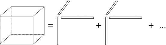
The parallel factor analysis (parafac) is a multilinear analogue of svd used in latent semantic analysis. The key idea is to minimize the sum of squares between the original tensor and the factorized model of the tensor. For the three mode case of a tensor ℐ ∈ ℝD 1 × D 2 × D 3 this gives the objective function in 13, where k is the number of dimensions in the factorized model (recall that ○ denotes the outer product):

The factorization algorithm finds a tensor (as a sum of rank one tensors) that is as similar as possible to the original tensor in the least squares sense, but has a fixed lower rank k: it is the best possible low-rank approximation of the original tensor for rank k.
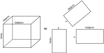
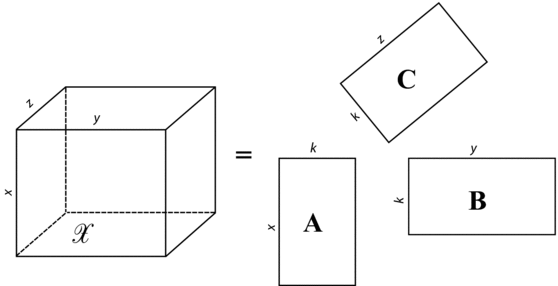
The algorithm results in three matrices, indicating the loadings of each mode on the factorized dimensions. The model is graphically represented in Figure 11, visualizing the fact that the parafac decomposition consists of the summation over the outer products of n (in this case three) vectors.
Graphical representation of parafac as the sum of outer products.
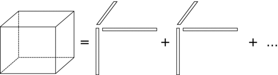
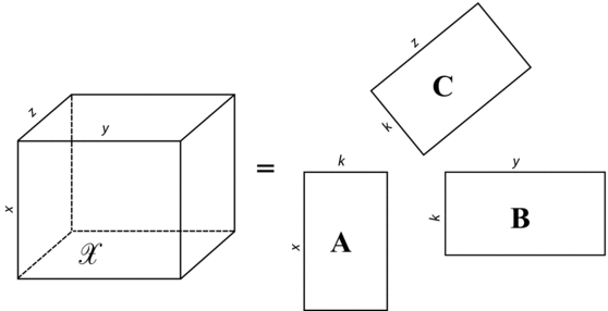
Figure 12 represents the factorization as three loading matrices, containing the loadings on each factor for the three different modes. The representation is equivalent to the representation with the sum of outer products – it differs only conceptually.
Graphical representation of parafac as three loading matrices.
There are a number of algorithms available to calculate the parafac decomposition. The most popular one is the alternating least squares method (als), which was proposed in the original papers by Carroll and Chang (Reference Carroll and Chang1970) and Harshman (Reference Harshman1970). In each iteration, two of the modes are fixed and the third one is fitted in a least squares sense. This calculation is done for each mode in turn, and the process is repeated until convergence.
3.3.2 Non-negative tensor factorization
Our second multi-way factorization is called the non-negative tensor factorization (ntf), it is the generalization of the non-negative matrix factorization for multi-way data. The ntf model is similar to the parafac analysis, with the constraint that all data needs to be non-negative (i.e. ≥ 0). This yields the objective function in (14):

As with the parafac model, the algorithm results in three matrices, indicating the loadings of each mode on the factorized dimensions.
There are again a number of ways to compute the factorization. Bro and Jong (Reference Bro and De Jong1997) use an alternating least squares algorithm similar to the als algorithm for parafac, but with some adaptations to enforce non-negativity. The non-negativity can be enforced by using a non-negative least squares computation, based on Lawson and Hanson (Reference Lawson and Hanson1974).Footnote 4 Another possibility is to use multiplicative update rules – similar to the update rules for non-negative matrix factorization, explained in Section 2.2.1 (Welling and Weber Reference Welling and Weber2001).
4 Application
4.1 Three-way selectional preferences
The model can straightforwardly be applied to language data. In this part, we describe the factorization of verbs × subjects × direct objects co-occurrences, but the example can easily be substituted with other co-occurrence information. Moreover, the model need not be restricted to three modes; it is very well possible to go to four modes and beyond – as long as the computations remain feasible.
The ntf decomposition for the verbs × subjects × direct objects co-occurrences into the three loading matrices is graphically represented in Figure 13. By applying the ntf model to three-way (s, v, o) co-occurrences, we want to extract a generalized selectional preference model, and eventually even induce some kind of frame semantics (in the broad sense of the word).
Graphical representation of ntf for language data.

In the resulting factorization, each verb, subject and direct object get a loading value for each factor dimension in the corresponding loadings matrix. The original value for a particular (s, v, o) triple xsvo can then be reconstructed with (15):
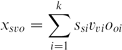
To reconstruct the selectional preference value for the triple (man, bite, dog), for example, we look up the subject vector for man, the verb vector for bite and the direct object vector for dog. Then, for each dimension i in the model, we multiply the ith value of the three vectors. The sum of these values is the final preference value.
4.2 Methodological remarks
The approach described in the previous section has been applied to Dutch, using the Twente Nieuws Corpus (Ordelman Reference Ordelman2002), a 500-million words corpus of Dutch newspaper texts. The corpus has been parsed with the Dutch-dependency parser Alpino (van Noord Reference van Noord, Mertens, Fairon, Dister and Watrin2006),Footnote 5 and three-way co-occurrences of verbs with their respective subject and direct object relations have been extracted. As dimension sizes, the 1kmost frequent verbs were used, together with the 10k most frequent subjects and 10k most frequent direct objects, yielding a tensor of 1k × 10k × 10k. The resulting tensor is very sparse, with only .02 percent (1/5,000 th) of the values being non-zero.
The tensor has been adapted with a straightforward extension of pointwise mutual information (Church and Hanks Reference Church and Hanks1990) for three-way co-occurrences, following (16). Negative values are set to zero.Footnote 6

The resulting matrix has been factorized into k dimensions (varying between 50 and 300) with the ntf algorithm described in Section 3.3.2.
4.3 Examples
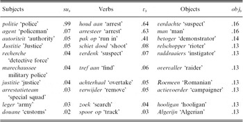
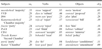
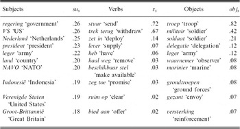
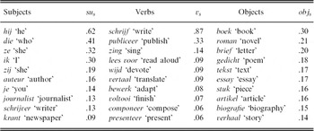
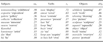
Tables 1 to 5 show example dimensions that have been found by the algorithm with k = 100. Each example gives the top 10 subjects, verbs and direct objects for a particular dimension, together with the score for that particular dimension. These example dimensions are given to illustrate the model's ability to extract an initial form of frame semantics.
Top 10 subjects, verbs and direct objects for the ‘police action’ dimension

Top 10 subjects, verbs and direct objects for the ‘legislation’ dimension

Top 10 subjects, verbs and direct objects for the ‘war movement’ dimension

Top 10 subjects, verbs and direct objects for the ‘publishing’ dimension

Top 10 subjects, verbs and direct objects for the ‘exhibition’ dimension

Table 1 shows the induction of a ‘police action’ frame, with police authorities as subjects, police actions as verbs and patients of the police actions as direct objects.
In Table 2, a legislation dimension is induced, with legislative bodies as subjects,Footnote 7 legislative actions as verbs and mostly law (proposals) as direct objects. Note that some direct objects (e.g. minister) also designate persons that can be the object of a legislative act.
Table 3 depicts a dimension of ‘war deployment’. The dimension contains military powers (countries, military organizations and leaders) that deploy (or remove) some form of military force.
Table 4 shows a ‘publishing’ dimension. The subjects contain writers (persons and bodies), who publish (in a broad sense) textual works.
Table 5, finally, is clearly an exhibition dimension, with verbs describing actions of display and trade that art institutions (subjects) can perform with works of art (objects).
These are not the only sensible dimensions that have been found by the algorithm. A quick qualitative evaluation indicates that about 44 dimensions contain similar, framelike semantics. In another 43 dimensions, the semantics are less clear-cut (single verbs or expressions account for one dimension, or different senses of a verb get mixed up). Thirteen dimensions are not very much based on semantic characteristics, but rather on syntax (e.g. fixed expressions and pronomina).
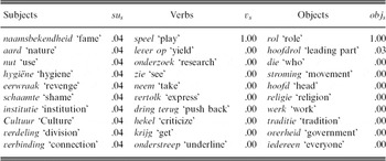
The qualitative evaluation indicates that some dimensions indeed do not contain framelike semantics, but those do contain information that may be useful for selectional preference induction. Such a dimension is shown in Table 6. It shows an example dimension in which practically all of the dimension's mass is attributed to one particular expression: een rol spelen, ‘to play a role’. The subject slot is more spread out: different kind of things might play a role – each with a fairly low probability.
Top 10 subjects, verbs and direct objects for the ‘play a role’ dimension

5 Evaluation
5.1 Evaluation framework
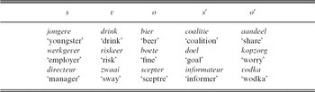
The results of the ntf model have been quantitatively evaluated in a pseudo-disambiguation task, similar to the one used by Rooth et al. (Reference Rooth, Riezler, Prescher, Carroll and Beil1999). It is used to evaluate the generalization capabilities of the algorithm. The task is to judge which subject (s or s′) and direct object (o or o′) is more likely for a particular verb v, where (s, v, o) is a combination drawn from the corpus, and s′ and o′ are a subject and direct object randomly drawn from the corpus. A triple is considered correct if the algorithm prefers both s and o over their counterparts s′ and o′ (so the (s, v, o) triple – that appears in the test corpus – is preferred over the triples (s′, v, o′), (s′, v, o) and (s, v, o′), according to (15)). Table 7 shows three examples from the pseudo-disambiguation task.
Three examples from the pseudo-disambiguation evaluation task's test set

Four different models have been evaluated. The first two models are tensor factorization models. The first model is the ntf model, as described in Section 3.3.2. The second model is the original parafac model, without the non-negativity constraints.
The other two models are matrix factorization models. The third model is the nmf model, and the fourth model is the svd model. For these models, a matrix has been constructed that contains the pairwise co-occurrence frequencies of verbs by subjects as well as direct objects. This gives a matrix of 1k verbs by 10k subjects + 10k direct objects (1k × 20k). The matrix has been adapted with pointwise mutual information.
The models have been evaluated with 10-fold cross-validation. The corpus contains 298,540 different (s, v, o) co-occurrences. Those have been randomly divided into ten equal parts. So in each fold, 268,686 co-occurrences have been used for training, and 29,854 for testing.
5.2 Evaluation results
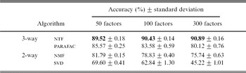
The accuracy results of the evaluation are given in Table 8. The results clearly indicate that the ntf model outperforms all the other models. The model achieves the best result with 300 dimensions, but the differences between the different ntf models are not very large – all attaining scores around 90 percent.
Results of the 10-fold cross-validation for the ntf, parafac, nmf and svd model for 50, 100 and 300 factors (averages and standard deviation)

The parafac results indicate the fitness of tensor factorization for the induction of three-way selectional preferences. Even without the constraint of non-negativity, the model outperforms the matrix factorization models, reaching a score of about 85 percent. The model deteriorates when more dimensions are used.
Both matrix factorization models perform worse than their tensor factorization counterparts. The nmf model still scores reasonably well, indicating the positive effect of the non-negativity constraint. The simple svd model performs worst, reaching a score of about 70 percent with fifty dimensions.
6 Conclusion and future work
This paper has presented a novel method that is able to investigate three-way co-occurrences. Other distributional methods deal almost exclusively with pairwise co-occurrences. The ability to keep track of multi-way co-occurrences opens up new possibilities and brings about interesting results. The three-way factorization methods are able to generalize among the data and overcome data sparseness.
The method has been applied to the problem of selectional preference induction. The results indicate that the algorithm is able to induce selectional preferences, leading to a broad kind of frame semantics. The quantitative evaluation shows that the use of three-way data is clearly beneficial for the induction of three-way selectional preferences. The tensor models outperform the simple matrix models in the pseudo-disambiguation task. The results also indicate the positive effect of the non-negativity constraint: both models with non-negative constraints outperform their non-constrained counterparts.
The results and the evaluation indicate that the method presented here is a promising tool for the investigation of nlp topics, although more research and thorough evaluation are desirable.
There is quite some room for future work. First of all, we want to further investigate the usefulness of the method for selectional preference induction. One of the most important extensions is the inclusion of other dependency relations in our model, apart from subjects and direct objects (thus making use of tensors with more than three modes).
Secondly, there is room for improvement and further research with regard to the tensor factorization model. The model presented here minimizes the sum of squared distance. This is, however, not the only objective function possible. Another possibility is the minimization of the Kullback–Leibler divergence. Minimizing the sum of squared distance normally assumes distributed data, and language phenomena are rarely normally distributed. Other objective functions – such as the minimization of the Kullback–Leibler divergence – might be able to capture the language structures much more adequately. We specifically want to stress this second line of future research as one of the most promising and exciting ones.
Finally, the model presented here is not only suitable for selectional preference induction. There are many problems in nlp that involve three-way co-occurrences. In future work, we want to apply the ntf model presented here to other problems in nlp, the most important one being word sense discrimination.
Acknowledgments
Brett Bader kindly provided his implementation of non-negative tensor factorization for sparse matrices, from which this research has substantially benefited. Anonymous reviewers provided fruitful comments and remarks on this paper, which considerably improved its quality.