, where n
1 Introduction
We present an algorithmic solution to the consistency problem for regular tree languages (i.e. languages recognised by finite tree automata). This inference task was first introduced by Gold (Reference Gold1978) under the name learning from given data. The objective is to identify a language that is known to be realisable by a finite automaton, but the necessary number of states is not known. Only a finite amount of data is available, and as opposed to query learning, the algorithm has no choice about the data. It is therefore impossible to prove that a pair of trees belong to the same congruence class. This means that even under the added restriction that the representation of the unknown language should be minimal with respect to some normal form (e.g. deterministic or residual automata), a given instance may have several nonequivalent solutions.
The inference algorithm in Section 3 takes as input two disjoint finite sets of trees 𝒫 and 𝒩, and outputs a finite tree automaton (FTA) that is consistent with 𝒫 and 𝒩 in that it accepts every tree in 𝒫 and rejects every tree in 𝒩.Footnote 1 To obtain a compact representation, the algorithm uses a heuristics similar to bisimulation minimisation (Buchholz Reference Buchholz2008). The algorithm is randomised, so executing it several times on the same input may yield nonequivalent automata. In this case, each output automaton typically represents a nontrivial generalisation of the examples in 𝒫 and 𝒩. Since the output automata are not restricted to a normal from, the algorithm does not convergence when the input sample is expanded and is therefore not useful for in-the-limit learning.
Owing to the close connection between context-free grammars and finite tree automata, the algorithm may be useful in natural language processing: it is well known that every context-free string language is the yield of a regular tree language. Finite automata usually offer a more succinct form of representation than corpora and are better suited for algorithmic processing. By using domain-specific knowledge to guide the nondeterministic choices made in the algorithm, it may be possible to find interesting generalisations from the input sample. Over-generalisation can be countered by supplying additional negative examples, either online or after termination and then resuming computation.
Whether or not the algorithm of Section 3 works with annotated data depends on the context. Seen as an inference algorithm for regular tree languages, it does not. Seen as an inference algorithm for context-free grammars, it does because from this point of view the input sets contain structurally annotated strings.
1.1 The consistency problem
The notion of learning from given data was introduced to provide insight into the in-the-limit learning model (Gold Reference Gold1967). Because of this historical setting, many algorithmic solutions to the consistency problem are designed to infer a target language in the limit. Our discussion of related work will therefore begin with a brief introduction to the in-the-limit learning model.
An algorithm (henceforth, the learner) is to infer a formal representation of a language . It is known that is a subset of a countable domain 𝒰 and belongs to a class of languages 𝒞. A problem instance builds upon an enumeration of 𝒰. The learner is revealed membership information about the elements in 𝒰 in the order dictated by , and must, after processing each item in the enumeration, guess the identity of . The class 𝒞 is learnable in the limit (from positive and negative data) if there is a learner with the following property. For every in 𝒞 and enumeration of 𝒰, there is a finite index i such that after processing the first i elements with respect to , the learner will always make the same guess, and it will be correct.
An equivalent definition can be made in terms of the consistency problem. The class 𝒞 is learnable in the limit if there is a consistency algorithm 𝔏 and a mapping f 𝔏 : 𝒞 → pow𝒰 such that for every ∈ 𝒞 and finite disjoint sets 𝒫, 𝒩 ⊆ 𝒰 with 𝒫 ⊆ , 𝒩 ∩ = ∅, and f 𝔏() ⊆ 𝒫 ∪ 𝒩, the algorithm 𝔏 returns a representation of on input 𝒫 and 𝒩. In this case, f 𝔏() is a characteristic set for .
It is known that unless P = NP there is no polynomial-time algorithm that finds a minimal deterministic finite automaton (DFA) A that is consistent with 𝒫 and 𝒩. The problem cannot even be efficiently approximated because computing a DFA that is only polynomially larger than A is also NP-hard (Pitt and Warmuth Reference Pitt and Warmuth1989). The difficulty is that to synthesise A, missing data must be guessed, and the hypothesis space is exponential in the size of 𝒫 ∪ 𝒩. On the other hand, computing an arbitrary consistent DFA takes only linear time, but this approach yields unnecessarily large automata and does not allow for identification in the limit.
The above observation is the basis for the timid state characterisation algorithm that infers regular languages in the limit with polynomial time and data (Gold Reference Gold1978). To compute a conjecture for 𝒫 and 𝒩, Gold's algorithm searches for subsets 𝒫0 ⊆ 𝒫 and 𝒩0 ⊆ 𝒩 from which a DFA A can be synthesised without having to guess missing data. If A is consistent with 𝒫 and 𝒩, then it becomes the next conjecture. If no such A can be obtained, then a prefix tree acceptor for 𝒫 is used as a dummy conjecture. In essence, the learner waits for a characteristic set for the target language and disregards data which it cannot use easily (Gold Reference Gold1978).
Gold's work inspired the search for polynomial-time consistency algorithms that produce small automata also when conditions are less than perfect, i.e. when the input data does not contain a characteristic set. Early attempts inferred deterministic automata by building a prefix tree acceptor matching the positive examples, and then merging as many states as possible while still respecting the negative examples. The first algorithm of this kind was given by Trakhtenbrot and Barzdin (Reference Trakhtenbrot, Barzdin and Louvish1973). The state-merge technique for DFA was later refined to obtain the regular positive and negative induction algorithm (Oncina and Garcia Reference Oncina, Garcia, de la Blanca, Sanfeliu and Vidal1991), which was further developed into the control strategy blue-fringe (Lang, Pearlmutter and Price Reference Lang, Pearlmutter, Price, Honavar and Slutzki1998). An extension of the technique to tree automata has been given by Garcia and Oncina (Reference Garcia and Oncina1993).
The question naturally arose whether the ideas used for inference of deterministic automata could be generalised to solve the consistency problem also for nondeterministic automata. A first step in this direction was made possible by the introduction of residual finite state automata by Denis, Lemay and Terlutte (Reference Denis, Lemay, Terlutte, Ferreira and Reichel2001). A residual finite state automata is a restricted type of nondeterministic finite automata that shares many nice algorithmic properties with DFA. For example, every regular language is recognised by a canonical residual finite state automata which has a minimal number of states and a maximal number of transitions. Denis, Lemay and Terlutte (Reference Denis, Lemay, Terlutte and Oliveira2000) have also presented a state-merge algorithm that infers residual finite state automata in the limit. The unambiguous finite automata constitute another class of mildly nondeterministic finite automata that was first studied by Schmidt (Reference Schmidt1978). The class of languages recognisable by unambiguous finite automata can also be learnt from given data, again by merging states in a prefix automaton (Coste and Fredouille Reference Coste, Fredouille, Lavrac, Gamberger, Todorovski and Blockeel2003).
The consistency problem for unrestricted (i.e. fully nondeterministic) finite automata is treated by de Parga, García and Ruiz (Reference de Parga, García, Ruiz, Ibarra and Yen2006). The authors present a family of in-the-limit algorithms that use maximal automata and state merging to infer regular languages. The work is continued by García et al. (Reference García, de Parga, Álvarez, Ruiz, Ibarra and Ravikumar2008) who present two variations on the stochastic order-independent learning algorithm (OIL): Minimal and Voting OIL. Both variations use the fact that OIL returns several output automata for a given input, but whereas Minimal OIL returns the smallest automaton, Voting OIL keeps all of them and uses a voting procedure to classify test samples. The algorithm presented in Section 3 differs from the OIL family in that it is based on partition refinement rather than state merging, and thus intuitively searches the hypothesis space in the opposite direction.
1.2 Learning tree languages and context-free grammars
Several learning algorithms for finite tree automata rely on access to a minimal adequate teacher, as introduced by Angluin (Reference Angluin1987). In this model, the algorithm is informed about the target language by querying a minimal adequate teacher oracle. The oracle is capable of answering membership and equivalence queries. Membership queries are of the form Is the tree t in ? and are answered with a yes or no. Equivalence queries are phrased Does the finite automaton A recognise ? and are answered with an element in the symmetric difference of (A) and , or with an acknowledgement that has been correctly identified if no such tree exists. The learning algorithm can thus use the oracle to sharpen its hypothesis until the right answer has been found. For regular tree languages, the minimal deterministic FTA that recognises can be inferred in polynomial time (Drewes and Högberg Reference Drewes and Högberg2007). There are also algorithms that infer deterministic weighted tree automata (Drewes and Vogler Reference Drewes and Vogler2007; Maletti Reference Maletti, Bozapalidis and Rahonis2007). A minimal adequate teacher algorithm for nondeterministic weighted tree automata over fields has been presented by Habrard and Oncina (Reference Habrard, Oncina, Sakakibara, Kobayashi, Sato, Nishino and Tomita2006). The algorithm uses the nice and somewhat surprising fact that weighted automata over fields have a Myhill-Nerode-like theorem of their own. For further reading, we recommend the survey of minimal adequate teacher algorithms that learn tree automata by Drewes (Reference Drewes2009).
A related learning model, also by Angluin (Reference Angluin1981), is learning from positive examples and membership queries. In this model, the oracle can only answer membership queries, but in addition to the oracle, the learning algorithm has access to a finite set 𝒫 ⊆ . In Besombes and Marion (Reference Besombes and Marion2007), the authors present a learning algorithm for regular tree languages that produces the unique minimal deterministic FTA A that recognises in polynomial time, provided that 𝒫 is a representative set for . A subset 𝒫 of is a representative set for if, after running A on every tree in 𝒫, every transition in A has been applied at least once.
In syntax-based computational linguistics, human language is processed based on its parse structure with respect to some formal grammar (Knight and May Reference Knight, May, Droste, Kuich and Vogler2009). An important learning task within this subfield is to derive a small context-free grammar that is consistent with a treebank, i.e. a set of labelled phrase-structure trees. This can be done through rule extraction, where the trees are divided into fractions representing productions in the output grammar. As shown by Bod (Reference Bod and Delmonte1999), rule extraction can be used to infer stochastic grammars from treebanks.
A different approach is suggested by Sakakibara and Muramatsu (Reference Sakakibara, Muramatsu and Oliveira2000) who present a genetic algorithm for inferring context-free grammars from (partially structured) positive and negative samples. The algorithm organises a maximal set of nonterminals in a table similar to that used in chart parsing and then uses a genetic-algorithm-based technique to merge nonterminals, so as to obtain a small output grammar.
The automatic distillation of structure algorithm derives a language from a positive sample of unannotated sentences by searching for sequential patterns in the data. Whereas automatic distillation of structure uses statistical analysis to structure and generalise from the input sample, our algorithm (in the context of string languages) additionally requires structural annotation and a negative sample to compute a representation that may generalise more strongly from the given input (Edelman et al. Reference Edelman, Solan, Horn, Ruppin, Brugo, Clark-Cotton and Ha2005).
A polynomial time in-the-limit algorithm that infers substitutable context-free languages from positive examples has been presented by Clark and Eyraud (Reference Clark, Eyraud, Jain, Simon and Tomita2005). A context-free string language is substitutable if the existence of strings u, v, l and r such that lvr, lur ∈ implies that l′ur′ ∈ ⇔ l′vr′ ∈ for all strings l′ and r′. This corresponds to Harris' (Reference Harris1951) principle that if a pair of word sequences constitute the same grammatical category, then they can be interchanged in any sentence without altering the grammatical correctness of the sentence. Harris' principle is also the foundation for alignment-based learning, an inference framework for unsupervised learning. Alignment-based learning algorithms typically operate in two phases. In the first phase, sample sentences are aligned to generate a set of hypotheses, each suggesting that a pair of sub-sentences constitute the same grammatical category. In the second phase, the most probable combination of hypothesis is selected through an expectation-maximisation search (van Zaanen Reference van Zaanen2001; Geertzen and van Zaanen Reference Geertzen, van Zaanen, Paliouras and Sakakibara2004).
The algorithm Emile learns a shallow context-free language in the limit from set of positive examples. A context-free language is shallow if it is generated by a grammar G such that every production in G is used in to generate at least one sentence of a length that is logarithmic in the size of G. Emile works by dividing and recombining the sample sentences, so as to discover syntactical categories. For efficiency reasons, some presentations of the algorithm include a membership oracle that can answer whether a given combination of sentence fragments is grammatically correct (Adriaans Reference Adriaans1999; Adriaans, Trautwein and Vervoort Reference Adriaans, Trautwein and Vervoort2000).
2 Preliminaries
This section reviews common notions and notations from tree automata theory. For an introduction to the field, see e.g. the survey by Comon et al. (Reference Comon, Dauchet, Gilleron, Jacquemard, Lugiez, Tison and Tommasi1997).
2.1 Sets and numbers
The set of real numbers is denoted by and the set of natural numbers (including 0) by . The subset {1, 2, . . ., n} of is abbreviated by [n]. Note that [0] = ∅. Let S be a set. The power set of S is denoted as pow(S), and we write S 2 as a short form for S × S. The set of all finite sequences (or strings) over S, including the empty sequence ᵋ, is S*. As usual, we denote the concatenation of strings u and v by the juxtaposition uv. The cardinality of the set S and the length of the string w ∈ S* are denoted by |S| and |w|, respectively.
2.2 Trees
A ranked alphabet is a finite nonempty set  of symbols which is partitioned into pairwise disjoint subsets Σ(k). The symbols in Σ(k) are said to have rank k. We will write f ∈ Σ(k) as f (k) if the rank cannot easily be determined from the context. The set T Σ of all trees over Σ consists of all mappings t:nodes(t)→Σ (called trees) with the following properties:
• The set nodes(t) is a finite prefix-closed subset of *.
• For every v∈nodes(t), if t(v) ∈ Σ(k) then {i∈|vi∈nodes(t)} = [k].
The set nodes(t) is called the nodes of t. The size of t, denoted |t|, is |nodes(t)|.
For a tree t ∈ T Σ and a node v∈nodes(t), the subtree of t rooted at v is denoted by t/v. It is defined by nodes(t/v) = {v′∈*|vv′ ∈ nodes(t)} and, for every v′ ∈ nodes(t/v), (t/v)(v′) = t(vv′). The subtrees of t, denoted subtrees(t), is the set of trees {t/v | v ∈ nodes(t)}. When S is a set of trees, subtrees(S) denotes ∪t ∈ Ssubtrees(t). A leaf of t is a node v such that t(v) is of rank 0. We shall denote a tree t as f[t 1, . . ., tk] if t(ᵋ) = f (k) and t/i = t i for 1≤ i ≤ k. Here, we say that the trees t 1, . . ., tk are direct subtrees of t. In the special case where k = 0 (i.e. nodes(t) = {ᵋ}), the brackets may be omitted, thus denoting t as f. A subset of T Σ is called a tree language.
We also need an operation that lets us replace a direct subtree of a tree with another tree. Given a pair of trees t = f[t 1, . . ., tk], t′ ∈ T Σ and an index i ∈ [k], we denote by t〚i ← t′〚 the tree f[t 1, . . ., t i−1, t′, t i+1, . . ., tk].
2.3 Finite automata
A FTA is a tuple A = (Q,Σ,δ,F) where Q is a finite nonempty set of states, Σ is a ranked alphabet of input symbols, δ = (δf)f ∈ Σ is a Σ-indexed family of mappings δf (k) : Q k → pow(Q), and F ⊆ Q is a set of final states. The FTA A is deterministic if, for every symbol f ∈ Σ(k) and sequence of states q 1, . . ., qk ∈ Q, it holds that |δf(q 1, . . ., qk)| ≤ 1. As usual, we extend δf to a mapping by letting δf pow(Q)f → pow(Q) by letting δf (Q1, . . ., Qk = ∪q1 ∈ Q1, . . . qk ∈ Qk δf(q 1, . . ., qk). We henceforth identify δf with its extension δf. The size of A, written |A|, is the sum of |Q| and the size of a sparse representation of δ.
A run of the FTA A on a tree t ∈ T Σ is a mapping r : nodes(t) → Q, such that r(v) is in the set δt(v)(r(v1) ċ r(vk)) for every node v ∈ nodes(t). The set of all runs of A on t is denoted as runs A(t). A run is accepting if r(ᵋ) ∈ F. The automaton A accepts a tree t if there is an accepting run of A on t. The language recognised by A, denoted (A), is the set of all trees that A accepts. A state q ∈ Q is reachable if there is a tree t ∈ T Σ, a run r ∈ runs A(t) and a node v ∈ nodes(t), such that r(v) = q. If, for some such r, r(ϵ) ∈ F then q is also live. A tree language L is a regular tree language if there is an FTA A such that L = (A).
2.4 Partitions
Let S be a set, and let and ′ be equivalence relations on S. We say that is a refinement of ′ if ⊆ ′, and that is a proper refinement of ′ if ⊂ ′. The equivalence class (or block) of an element s ∈ S with respect to is the set [s] = {s′ |(s,s′) ∈ }. It should be clear that [s] and [s′] are equal if and only if s and s′ are in relation , and disjoint otherwise, so induces a partition (S/) = {[s] | s ∈ S} of S.
3 The inference algorithm
In this section, we present an algorithm that takes as input a pair of disjoint finite nonempty sets of trees 𝒫 and 𝒩 and outputs an FTA A such that 𝒫 ⊆ (A) ⊆ (T Σ \ 𝒩). During its execution, the algorithm iteratively refines an equivalence relation on the set subtrees(𝒫). From each intermediate relation, a hypothesis automaton A 𝒫 is compiled using the construction in Definition 3.1.
Definition 3.1. (Synthesised FTA)Let 𝒫 be a finite subset of T Σand be an equivalence relation on subtrees(𝒫) that refines {(s 1, s 2) | s 1 ∈ 𝒫 ⇔ s 2 ∈ 𝒫}. The FTA synthesised from and 𝒫 is A 𝒫 = (Q, Σ, δ, F), where Q = (subtrees(𝒫)/), F = {q ∈ Q | q ⊆ 𝒫} and

for every symbol f (k) ∈ Σ and sequence of states q 1, . . ., qk ∈ Q. □
By the subtree-closedness of subtrees(𝒫), the state [t] is reachable on t, for every t ∈ subtrees(𝒫). From this property, which is easy to prove by induction, it follows that A 𝒫 is consistent with 𝒫.
Lemma 3.2Let , 𝒫 and A 𝒫be as in Definition 3.1. For every t ∈ subtrees(𝒫), there is a run r ∈ runs A 𝒫(t) such that r(ᵋ) = [t].
Corollary 3.3 𝒫 ⊆ (A 𝒫).
We note that if is the identity relation, then A 𝒫 is a prefix-tree acceptor for 𝒫, i.e. a loop-free deterministic FTA with |subtrees(𝒫) states that accepts precisely the trees in 𝒫. It is clear that a coarser equivalence relation will yield a smaller output automaton, but usually at the cost of a recognising a larger language.
This trade-off between size and precision makes an iterative approach appealing, that also makes use of a set 𝒩 of negative examples. The idea is to start with a very coarse relation that only distinguishes between trees in 𝒫 and trees in subtrees(𝒫) \ 𝒫 (as in Definition 3.1). If A 𝒫 accepts a tree s in 𝒩, then the relation is refined to reduce the number of accepting runs of A 𝒫 on s. This process is repeated until A 𝒫 rejects every tree in 𝒩.
Assume that A 𝒫 has an accepting run r on s ∈ 𝒩. To find an appropriate refinement of , we search r for a transition that is only available in A 𝒫 because has placed a pair of distinct trees in the same equivalence class. A transition of this type is called a generalisation. The easiest way to find a generalisation is to traverse s bottom-up, selecting the first node v in nodes(s) such that s/v = f (k)[t 1, . . ., tk] is not in r(v), but ti is in r(vi) for every i ∈ [k]. Such a v must exist, because otherwise s ∈ r(ᵋ) ⊆ 𝒫 which contradicts the disjointness of 𝒫 and 𝒩.
Since A 𝒫 could assign r(v) to v, we have r(v) ∈ δf(r(v1), . . ., r(vk)). This implies that there are trees t′i ∈ r(vi), i ∈ [k], such that f[t′ 1, . . ., t′k] ∈ r(v). To avoid that the transition from r(v1), . . ., r(vk) to r(v) on f is used to accept s, the relation is refined as follows.
We take the tree f[t′ 1, . . ., t′k] and start to replace the subtrees t′ 1, . . ., t′k with their counterparts in t 1, . . ., tk. The trees are replaced one by one, for as long as the resulting tree remains in r(v). We will not manage to replace all of them because then we would eventually have f[t 1, . . ., tk] ∈ r(v), which we know is not true. Let s″ = f[t″ 1, . . ., t″k] be result of this replacement process, and let i ∈ [k] be the index of one of the subtrees that were never replaced. We now divide r(vi) into two blocks, B 1 = {u ∈ r(vi) | s″〚i ← u〚 ∈ r(v)} and B 2 = {u ∈ r(vi) | s″〚i ← u〚 ∉ ∈ r(v)}. Clearly, t′i ∈ B 1 whereas ti ∈ B 2.
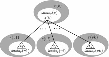
The run r typically contains several generalisations when is coarse. To identify the nodes gen(r) ⊆ nodes(s) at which they occur, we define the mapping basicr: nodes(s) → subtrees(𝒫) through structural induction on s, starting at the leaves. Let v ∈ nodes(s) with s/v = f[t 1, . . ., tk]. Intuitively, basicr(v) contains those trees that justify a transition from basicr(v1), . . ., basicr(vk) to r(v) on the symbol f (see Figure 1 for an illustration). If no such tree exists, then v uses a generalisation and should be added to gen(v). To find further generalisations, we let basicr(v) = r(v) and continue upwards. In the definition of gen and basicr below, we use the mapping basic′r as a technical convenience.
For every v ∈ nodes(s) with s(v) = f (k), the set basicr(v) ⊆ r(v) contains the trees that caused r(v) to be in δf(r(v1), . . ., r(vk)).

Definition 3.4 (Basis and generalisation)Let , 𝒫 and A 𝒫be as in Definition 3.1. Recall that the set of states of A 𝒫is (subtrees(𝒫)/). In addition, let t ∈ T Σand r ∈ runs A 𝒫(t). The mappings basicr, basic′r : nodes (t) → pow(T Σ) are inductively given, for every v ∈ nodes (t) with t(v) = f ∈ Σ(k), by

and

The set of generalisations in the run r, denoted gen(r), is the set of nodes {v ∈ nodes(t) | basic′r(v) = ∅}.
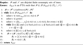
A formal presentation of the inference algorithm is given in Algorithm 1. After constructing an initial partition of subtrees(𝒫), the algorithm enters into the main loop. With each new iteration of the loop, the algorithm synthesises an FTA A 𝒫 from and 𝒫. If A 𝒫 has an accepting run on a tree in the negative corpus 𝒩, then the algorithm refines to cancel this particular run. It does this by identifying a block that is used in a generalisation and then splits the block using a local condition on the transition structure, similar to that of forward bisimulation (Buchholz Reference Buchholz2008). This process continues until A 𝒫 respects 𝒩. In the case when 𝒫 is subtree-closed, the initial relation has a single equivalence class and the algorithm terminates after one iteration.
Derive an FTA from given data

Before we prove that Algorithm 1 is correct, let us step through a run of the algorithm, so as to complement the theoretical presentation with a concrete example.
Example 3.5Suppose that Algorithm 1is invoked with input 𝒫, 𝒩 ⊂ T Σ, where
![\begin{linenomath}
\[
\begin{array}{@{}r@{\,}c@{\,}ll}
\Sigma {=} \{\; a^{(0)},\;\; b^{(0)},\;\; g^{(1)},\;\;\;\; f^{(2)} \; \} ,\\
\possamp {=} \{\, b,\;\,
f[a,a],\;\,
f[g[b],a],\;\,\;\;
f[g[b],g[f[b,a]]] \;\,
\} \textrm{ and }\\
\negsamp {=}
\{\,
g[a],\;\,
f[g[b],g[b]],\;\;\;\;
f[f[f[f[b,a],a],a],a] \,
\} .
\end{array}
\]
\end{linenomath}](https://static.cambridge.org/binary/version/id/urn:cambridge.org:id:binary:20151022070640754-0330:S1351324911000064_eqnU4.gif?pub-status=live)
With this input, the domain of is subtrees(𝒫) = 𝒫 ∪ {a, g[b], f[b,a], g[f[b,a]]}. After the initialisation step at line 1, the relation has the equivalence classes B 1 = 𝒫 and B 2 = subtrees(𝒫) \ 𝒫.
Upon entering the main loop at line 2, the algorithm synthesises an FTA from the partition induced by on its domain (the construction is given in Definition 3.1). The result is the automaton A 1 = ({B 1, B 2}, Σ, δ, {B 1}) with the transition mapping listed below.

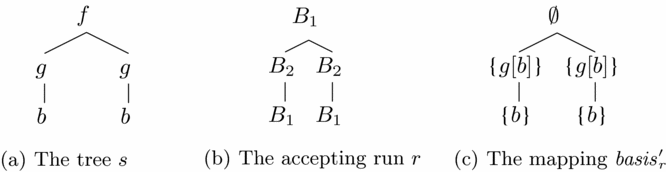
When applied to the trees in 𝒩, the automaton A 1correctly rejects g[a] but accepts the tree s = f[g[b],g[b]] (drawn in Figure 2a). The unique accepting run r of A 1on s is given in Figure 2(b). To find a way to cancel r, the algorithm computes the mappings basic′r and basicr. The mapping basic′r is shown in Figure 2(c); the mapping basicr is identical, except that for every node u ∈ nodes(s) such that basic′r(u) = ∅, we have basicr(u) = r(u). In this particular case, the only difference between basic′r and basicr is that basic′r(ᵋ) = ∅, whereas basicr(ᵋ) = r(ᵋ) = B 1.
The automaton A 1 accepts the tree s ∈ 𝒩 through the run r. To cancel r, Algorithm 1 computes the mapping basic′r.
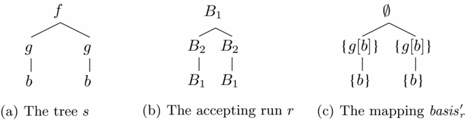
As the reader may recall, gen(r) contains every node u ∈ nodes(s) such that basic′r(u) = ∅. According to the computations in Figure 2(c), this means that gen(r) = {ᵋ}. Hence, Algorithm 1can only select v = ᵋ at line 4. At line 5, the tree t can be selected in more than one way. To continue, we assume that algorithm nondeterministically chooses t = f[a,a] ∈ B 1.
While traversing the loop at lines 6–7, the algorithm nondeterministically decides to replace the left subtree (i.e. t/1 = a) of t. It can only replace a with g[b] because g[b] is the only element in basicr(1). After this operation, the right subtree must be kept as it is because if we replace it with the unique tree g[b] ∈ basicr(2), then the resulting tree f[g[b],g[b]] is no longer in B 1. The inner loop consequently exits, and at line 8 the algorithm must choose i = 2.
By splitting the block r(vi) = r(ᵋ 2) = r(2) = B 2of with respect to t = f[g[b],a] and i = 2 (see lines 9–11 of Algorithm 1), a finer relation is obtained. This relation has the equivalence classes B 21 = {a, g[f[b,a]]}, B 22 = {g[b], f[b,a]} and
![\begin{linenomath}
\[
\bblock_{1} = \{b,\; f[a,a],\; f[g[b],a],\; f[g[b],g[f[b,a]]]\}.
\]
\end{linenomath}](https://static.cambridge.org/binary/version/id/urn:cambridge.org:id:binary:20151022070640754-0330:S1351324911000064_eqnU6.gif?pub-status=live)
The updated FTA A 2 = (B 1, B 21, B 22}, Σ, δ, {B 1}) is such that

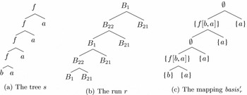
After the first completed iteration of the main loop, the algorithm returns to the head of the loop at line 2, were it runs A 2on the trees in 𝒩. This time, the automaton A 𝒫rejects both g[a] and f[g[b],g[b]], but it accepts the tree f[f[f[f[b,a],a],a],a] ∈ 𝒩 (drawn in Figure 3a) through the accepting run r shown in Figure 3(b). Again, the algorithm computes basicr yielding the function in Figure 3(c). At line 4, the algorithm can either choose v = ᵋ or v = 11 from gen(r). We assume that it chooses v = 11 and that it at line 5 selects t = f[g[b],a]. This is a permissible option since t/1 = g[b] ∈ r(v1) = r(111) = B 22and t/2 = a ∈ r(v2) = r(112) = B 21.
The automaton A 2 accepts the tree s ∈ 𝒩 through the run r. To cancel r, Algorithm 1 computes the mappings basic′r and basicr.

Let us see what these choices mean for the whileloop at line 6. It should be clear that the right subtree of t cannot be replaced because it is already in basicr(v2). The left subtree of t cannot be replaced either because f[g[b],a]〚1 ← f[b,a]〚 = f[f[b,a],a] is not in r(v) = r(11) = B 1. The whileloop thus exits immediately and the algorithm continues to split the block r(vi) = r(111) = B 22of with respect to t = f[g[b],a] and i = 1. This refinement produces a relation with the equivalence classes B 21 = {a, g[f[b,a]]}, B 221 = {g[b]}, B 222 = {f[b,a]} and
![\begin{linenomath}
\[
\bblock_{1} = \{\; b,\; f[a,a], \; f[g[b],a],\; f[g[b],g[f[b,a]]] \; \} .
\]
\end{linenomath}](https://static.cambridge.org/binary/version/id/urn:cambridge.org:id:binary:20151022070640754-0330:S1351324911000064_eqnU8.gif?pub-status=live)
Having completed the second iteration of the main loop, the algorithm re-computes the automaton A 𝒫. The result is the automaton A 3 = (Q, Σ, δ, F), where Q = {B 1, B 21, B 221, B 222}, F = {B 1} and δ is given by

Returning once more to line 2 and the head of the main loop, the algorithm runs A 3on every tree in 𝒩. As A 3rejects all of them, the main loop is exited, A 3is returned, and the algorithm terminates.
The final automaton A 3generalises from 𝒫 to an infinite language. This follows from the fact that A 3contains a loop (that goes through the transitions labelled † and ‡) and that, as we shall see later, every state in A 3is reachable and live.
3.1 Correctness
In preparation for the correctness proof, we demonstrate that certain invariants hold throughout the execution of the algorithm. The first step is to verify that the selections required by the main loop of Algorithm 1 are always feasible.
Lemma 3.6For every tree t ∈ T Σ \ 𝒫 and run r ∈ runs A 𝒫(t) such that r(ᵋ) ⊆ 𝒫, the set of nodes gen(r) is nonempty.
Proof
Assume that the conditions of Lemma 3.6 hold, but that gen(r) = ∅. It then follows that for every v ∈ nodes(t), the set basicr(v) = ′r(v) contains the subtree t/v of t rooted at v. Since basicr(v) ⊆ r(v), we obtain that t/ᵋ = t is in r(ᵋ), which in turn is a subset of 𝒫. Hence, t ∈ 𝒫 which contradicts t ∈ T Σ \ 𝒫. □
Invariant 3.7 The selections at lines 3, 4, 5 and 8 can always be made.
Proof
Since s ∈ (A 𝒫), there is a run r ∈ runs A 𝒫(s) such that r(ᵋ) ⊆ 𝒫. Furthermore, since s ∈ 𝒩, we know that s ∉ ∈ 𝒫, so by Lemma 3.6, gen(r) is nonempty.
The tree t of line 5 must exist since r(v) ∈ δf(r(v1), . . ., r(vk)), for otherwise r would not be in runs A 𝒫(s). After the while loop at lines 6 and 7, there is still at least one subtree ti of t such that ti ∉ ∈ basicr(vi), or else v would not be in gen(r), so the index sought at line 8 is guaranteed to exist. □
We continue to show that the refinement step of line 9 yields a proper refinement of the equivalence relation , thereby removing one source of over-generalisation. This result can then be used to prove that A 𝒫 contains no useless states.
Invariant 3.8The relation is always an equivalence relation on subtrees(𝒫), and in every iteration of the main loop, is properly refined.
Proof
The proof is by induction on the number of times Algorithm 1 iterates over the main loop. After the initialisation step at line 1, = 𝒫2 ∪ (subtrees(𝒫) \ 𝒫)2 is clearly an equivalence relation on subtrees(𝒫).
For the inductive step, we show the refinement step at lines 9–11, (i) preserves reflexivity, transitivity and symmetry; and (ii) divides the block r(vi) into two blocks B 1 = {ti′ ∈ r(vi) | t〚i ← ti′〚 ∈ r(v)} and B 2 = r(vi) \ B 1, such that basicr(vi) ⊆ B 2.
The correctness of Claim (i) follows immediately from the fact that is an equivalence relation and the definitions of B 1 and B 2 at lines 10 and 11.
Let us now verify Claim (ii). By definition, basicr(vi) ⊆ r(vi). If there was a tree ti′ ∈ basicr(vi) such that t〚i ← ti′〚 ∈ r(v), then this would contradict the satisfied termination criterion at line 6 and the choice of i at line 8 of Algorithm 1. It thus follows that basicr(vi) ∩ B 1 = ∅ and basicr(vi) ⊆ B 2.
For every u ∈ nodes(s), the set basicr(u) is nonempty (by Definition 3.4). In particular, basicr(vi) is nonempty and so is B 2 since it includes basicr(vi). Finally, we know that r ∈ runs A 𝒫(s), so there must be a ti′ ∈ r(vi) such that t〚i ← ti′〚 ∈ r(v), which means that also B 1 is nonempty. □
Invariant 3.9Every state in A 𝒫is reachable and live.
Proof
By Invariant 3.8, is an equivalence relation on subtrees(𝒫).
By Definition 3.1, the states Q of A 𝒫 are the equivalence classes of . By Lemma 3.2, every state [t] ∈ Q is reachable on t.
Let us also verify that q = [t] is live. As [t] ⊆ subtrees(𝒫), there is a tree s ∈ 𝒫 and a v ∈ nodes(s) such that s/v = t. It follows that there is a run of A 𝒫 on s such that r(ᵋ) = [s] and r(v) = [t], so r is accepting and [t] is live. □
Lemma 3.10 follows immediately from Invariant 3.8 and the finiteness of 𝒫.
Lemma 3.10Algorithm 1 terminates.
Corollary 3.3 in combination with the termination criterion at line 2 of Algorithm 1 yields Theorem 3.11.
Theorem 3.11Upon termination, 𝒫 ⊆ (A 𝒫) ⊆ (T Σ \ 𝒩).
3.2 Complexity
In the complexity analysis, the size of a set of trees 𝒳 is the sum of the sizes of its constituent trees. The sum ∑t ∈ 𝒳 |t| is denoted by n 𝒳 for 𝒳 ∈ {𝒫, 𝒩}. To obtain a safe upper bound, the nondeterministic algorithm is assumed to persistently make the worst possible choices. We omit average-time calculations as they require a deeper statistical analysis and depend on the distributions that generate 𝒫 and 𝒩.
Theorem 3.12The worst-case time complexity of Algorithm 1is in  .
Proof
An efficient implementation uses a directed acyclic graph representation of the set 𝒫. The directed acyclic graph can be initialised in  computation steps and requires no further maintenance. Each iteration of the main loop properly refines . Thus, after at most n iterations, the algorithm terminates. In each iteration, the algorithm synthesises A 𝒫 from and 𝒫, consuming O(n ) computation steps. By Theorem 1.7.3 of Comon et al. (Reference Comon, Dauchet, Gilleron, Jacquemard, Lugiez, Tison and Tommasi1997), deciding whether there is an accepting run of t in 𝒩 costs O(|A 𝒫| ċ |t|) steps, so finding any tree in 𝒩 with an accepting run r costs O(n 𝒫 ċ n 𝒩) steps. Computing gen(r) is almost equally expensive and is in O(n 𝒫 ċ |t|), which is bounded by O(n 𝒫 ċ n 𝒩), but this includes the selection of v, t and i. Finally, r(vi) can be split with respect to v, t and i in time n 𝒫 by taking advantage of the directed acyclic graph representation. The overall time complexity is thus . □
Theorem 3.12 reveals an asymmetry in the impact of n and n 𝒩 on the time complexity of Algorithm 1. For some applications, a complement automaton may be sufficient, i.e. an automaton that accepts every tree in 𝒩 and rejects every tree in 𝒫. When this is the case, we can find an automaton representation for our samples in O(min(n 𝒩 ċ n 𝒫2,n 𝒫 ċ n 𝒩2)) computation steps by running Algorithm 1 on input (𝒩, 𝒫) rather than (𝒫,𝒩) whenever n 𝒩 is smaller than n .
4 Experiments
To complement the theoretical results of Section 3, we implemented a prototype in Java. The prototype was executed on input samples ranging in size from 0 to 200 nodes, and the size of the output automaton and the total running time were recorded. The samples were obtained as follows: A set of trees was generated at random using a regular tree grammar G, such that (G) = T Σ, where Σ = {a (0), b (0), c (0), f (2), g (2), h (1)}. The set was then divided, again at random, into disjoint sets 𝒫 and 𝒩 (not necessarily of equal size). For each measuring point, 50 test runs were made and the average values computed.
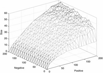
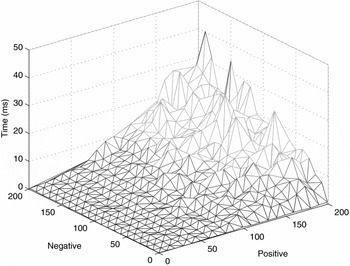
The results of the experiments are reported in Figures 4 and 5. The former shows the size of the output automaton as a function of the size of the input sample. In our tests, the output is typically smaller than the input, so for some applications the algorithm may provide a useful form of compression. Figure 5 shows the execution time of the prototype (when run on a MacBook with a 2.4 GHz Intel Core 2 Duo processor and 4 GB of memory), and the empirical results appear to support the theoretical prediction.
The size of the output automaton as a function of n and n 𝒩.

The running time of the prototype (in milliseconds) as a function of n and n 𝒩.

5 Future work
One direction for future work is to lift the family of algorithms described by de Parga et al. (Reference de Parga, García, Ruiz, Ibarra and Yen2006) to the domain of trees and to compare their performance with that of Algorithm 1. From a theoretical point of view, it would also be nice if Algorithm 1 could be modified to allow identification in the limit. One could of course fall back on the strategy employed by Gold (Reference Gold1978), begin each run of the algorithm by searching for a characteristic sample and, if it exists, generate a minimal deterministic automaton, but this hardly seems satisfying, and a solution based on a canonical form for nondeterministic FTA would be more appealing.
The complexity analysis in Section 3.2 supposes a worst-case scenario, and the experiments in Section 4 are made with randomly generated input sets. To better understand the appropriateness of Algorithm 1 for practical natural language processing applications, it would be useful to estimate the average-case time complexity and to conduct more extensive experiments on real-world data.
Acknowledgments
We thank the referees for their helpful comments and suggestions. We are also grateful to Henrik Björklund, Frank Drewes and Brink van der Merwe for reading and discussing the manuscript.