1 Introduction
This paper presents a unified algorithm for extracting translation correspondences from non-sentence-aligned bilingual data in the area of statistical machine translation (SMT). Originally, such algorithms have been proposed for parallel corpora, which can be aligned largely monotonically with no re-orderings and only limited insertions and deletions between the two sentence collections (Brown et al. Reference Brown, Lai and Mercer1991; Gale and Church Reference Gale and Church1991; Melamed Reference Melamed1999; Moore Reference Moore2002; Zhao and Vogal Reference Zhao and Vogel2002; Utiyama and Isahara Reference Utiyama and Isahara2003; Deng, Kumar and Byrne Reference Deng, Kumar and Byrne2006; Ma Reference Ma2006).
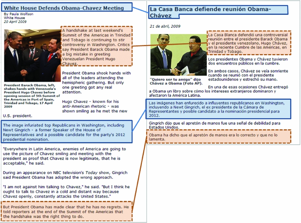
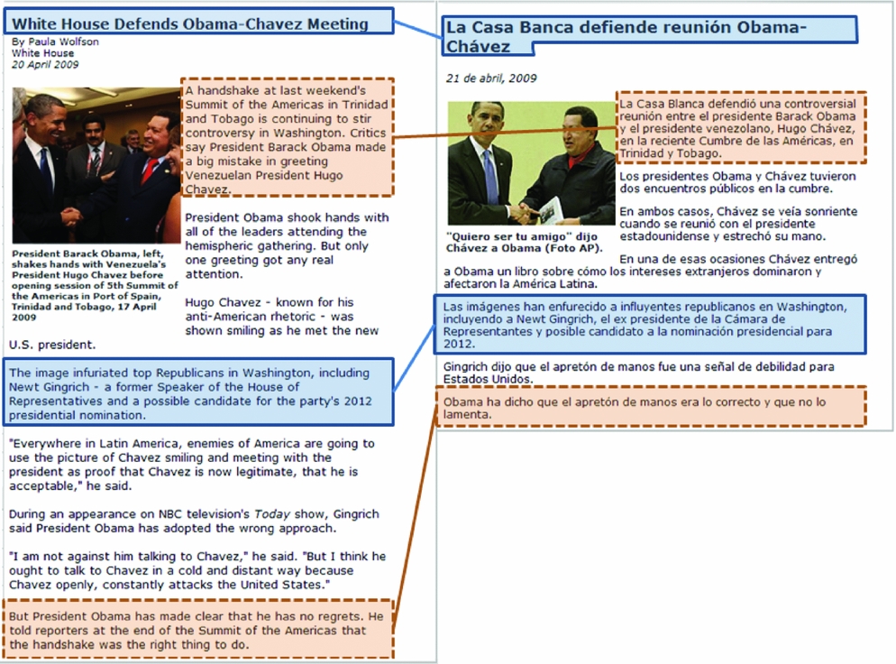
More recent work has focused on extracting parallel data from comparable noisy data. Here, the data might be processed at the document level (Snover, Dorr and Schwartz Reference Snover, Dorr and Schwartz2008), or the document-level processing is used as a pre-filtering step (Utiyama and Isahara Reference Utiyama and Isahara2003; Munteanu and Marcu Reference Munteanu and Marcu2005; Quirk, Udupa and Menezes Reference Quirk, Udupa and Menezes2007). In Munteanu and Marcu (Reference Munteanu and Marcu2005) and Quirk et al. (Reference Quirk, Udupa and Menezes2007), one-to-one sentence-level pairs are then derived from the document-aligned data. This sentence alignment can be further used to extract sub-sentential fragment pairs (Munteanu and Marcu Reference Munteanu and Marcu2006; Quirk et al. Reference Quirk, Udupa and Menezes2007). Figure 1 highlights these different levels of parallelism present in a typical comparable document pair: sentence level as well as sub-sentential translation correspondences. In the current paper, we present a single unified search implementation that can be used on all the different extraction tasks handled by various above-cited algorithms. As the degree of parallelism (e.g. parallel data, noisy parallel, or comparable data as defined by Fung and Cheung Reference Fung and Cheung2004) for given bilingual data might be unknown, the unified algorithm could be applied more flexibly.
Illustration of different levels of parallelism present in an English (left) and Spanish (right) comparable document pair. The sentences marked with solid lines are parallel sentences. The sentences marked with broken lines are not parallel, but contain sub-sentential fragments that are parallel. Both documents are from the Voice of America News (VOA News).
In this paper, translation pair extraction is handled as a chunk-alignment problem: No document-level pre-filtering is used and sentence-level pre-filtering is handled as a novel beam-search pruning step. For comparable data, the extraction of many-to-many translation pairs is included in a straight-forward way. Sub-sentential fragments are extracted with a smaller amount of pre-filtering than previous work. The unified algorithm uses techniques from large-scale dynamic programming (DP) beam-search algorithms in speech recognition (SR) (Ney Reference Ney1984): The search space is dynamically constructed, and just two stacks of active hypotheses or states are used to process the parallel data at word level. This way the algorithm is also similar to SMT decoding algorithms (Koehn Reference Koehn2004; Och and Ney Reference Och and Ney2004; Tillmann Reference Tillmann2006). In order to carry out the sentence alignment, the algorithm uses simple word-based features: lexical scoring features based on the so-called IBM Model-1 (Brown et al. Reference Brown, Della Pietra, Della Pietra and Mercer1993), coverage features, and similarity features based on character matching. These can be computed incrementally to support the beam-search extraction algorithm.
The main contribution of the current paper lies in a combination of techniques from previous work on extracting parallel data, stack-based decoding for SR, alignment algorithms for SMT, and the use of incrementally computed features for phrase-based SMT decoders. As a result, the classifier-based extraction algorithm can explore huge search spaces at an unprecedented scale. The paper is organized as follows: Section 2 presents the extraction task for various data conditions as a so-called link alignment problem, which is classified into different alignment types and link-type sets. The extraction task is formally compared to a pattern recognition formulation of the SR problem. Section 3 describes the feature-based link scoring model used in this paper. Section 4 demonstrates the unified stack-based search, which is the main contribution of this paper. This section presents detailed pseudo-code of the unified search, which depends on a careful stack-based implementation to maintain efficiency while being applicable to different alignment types. Section 5 presents details about the beam-search pruning as well as the efficient incremental feature computation. In Section 6, we show experimental results. Section 7 compares the unified algorithm with previous work in the literature and discusses future work.
2 Link sequence search problem
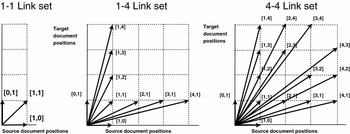
We extract bilingual pairs of text chunks: A chunk consists of a sequence of source or target words (Deng et al. Reference Deng, Kumar and Byrne2006). Chunk pairs are either sub-sentential fragment pairs, one-to-one, or many-to-many sentence-level pairs. We call an interval pair of source and target positions that corresponds to a chunk pair in a bitext a link. A bitext is a parallel text (Melamed Reference Melamed1999), which is indexed at the word level in the current paper. Even though we are interested in the words covered by a link, conceptually our algorithm computes a chunk pair alignment that constitutes a sequence of links. Based on a link, the words can always be recovered after the search has finished. For the experiments in Section 6, we consider 1-to-1, 1-to-4, and 4-to-4-type links at the sentence level as well as 10-to-10-type links at the word level when extracting sub-sentential fragment pairs. Here the numbers refer to the maximum link size in terms of sentences or words in the source or target side. The link concept is illustrated in Figure 2. For the 1-4-type links, a single sentence is aligned to up to four sentences in the other language (this restriction is used by Ma Reference Ma2006), i.e. this link set  contains nine types: = {1-0, 1-1, 1-2, 1-3, 1-4, 0-1, 2-1, 3-1, 4-1}. Here special ‘null’ links for insertions and deletions are included. Similarly, for the 4-to-4-type links up to four source and target sentences are aligned to each other. Here we exclude link types with the same length, i.e. 2-to-2, 3-to-3, and 4-to-4 links, as these can be handled by sequences of 1-to-1 links. Similarly, sub-sentential links consist of up to 10 source and target words. Link types can be handled flexibly at run time: they correspond to state expansions in the dynamically constructed search space.
Illustration of different link sets that are used in this paper. A link corresponds to a pair of text chunks that cover a certain number of sentences or words. During search, link sequences are extracted based on alignment coverage/continuity restrictions (see Figure 3 for an illustration). A link corresponds to a local transition between bitext (sentence or word) positions. A pattern recognition definition for link sequences is given in Section 2.1. 10-to-10-word level transitions for extracting sub-sentential fragments are not shown here.

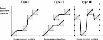
The search algorithm handles different degrees of sentence-level order differences between source and target texts. Different alignment types are handled jointly within a unified implementation. The alignment types are illustrated in Figure 3.
The unified algorithm handles three alignment types. Only one-to-one links are shown, but many-to-many links (see Figure 2) are handled uniformly across all alignment types. The search algorithm finds the shortest path through the bitext space. The path along with start and end point restrictions is shown as bold lines and points. For details, see Section 2.1.

Type I. Monotone search. In Brown et al. (Reference Brown, Lai and Mercer1991), Gale and Church (Reference Gale and Church1991), Chen (Reference Chen1993), Moore (Reference Moore2002), Zhao and Vogel (Reference Zhao and Vogel2002), and Ma (Reference Ma2006), the sentence alignment search is restricted to monotone alignments, which results in an efficient search algorithm. Our current constant memory algorithm carries out a full monotone search without pruning. The memory requirements are constant with respect to the source document length, but linear with respect to the target document length. The monotone search can be carried out at the sentence as well as word levels. The word-level search is used to compute a sub-sentential fragment alignment.
Type II. Sentence-level re-ordering search. A novel restricted sentence level re-ordering search is introduced. It uses a target coverage vector to handle some sentence-order differences in mostly monotone data. The search space is restricted by a local re-ordering window similar to the way a decoder for SMT handles word-level re-ordering. It can also be related to the binary search in Deng et al. (Reference Deng, Kumar and Byrne2006).
Type III. Comparable data search. When searching for sentence-level pairs in comparable data, no monotonicity assumption is made for source and target sentences. Typically, only one-to-one link pairs are extracted (Munteanu and Marcu Reference Munteanu and Marcu2005; Quirk et al. Reference Quirk, Udupa and Menezes2007; Tillmann and Xu Reference Tillmann and Xu2009). The current algorithm is capable of extracting many-to-many links as a straight-forward extension of the one-to-one link search.
If the source and target sentences are from a matching document pair, a monotone search or almost monotone search can be carried out (Type I and Type II defined above). If a document-level alignment is unavailable, e.g. for comparable data, a non-monotone Type III search is carried out. Here the set of target chunks considered as matches is restricted based on a publication date window (Munteanu and Marcu Reference Munteanu and Marcu2005): for a given source sentence S only those target sentences T are considered that have been published within a window of ± 3 days. The link search for sub-sentential fragment pairs is handled as a combination of the search for alignment Types I and III: We pre-match candidates at the sentence-level and carry out a monotone search within the candidate sentences. In comparison, Munteanu and Marcu (Reference Munteanu and Marcu2006) and Quirk et al. (Reference Quirk, Udupa and Menezes2007) extract fragments based on a two-step filtering pipeline: (1) matching document pairs are extracted based on an Information-Retrieval (IR) criterion; (2) from within the matching documents, sentence pairs are extracted based on a sentence-level matching criteria. Finally, sub-sentential fragments are extracted from these sentence pairs. In this paper, we all together skip the document-level pre-filtering, and formulate the sentence-level pre-filtering step as a special pruning step within the unified beam-search algorithm: even sub-sentential fragment extraction is carried out in a single run over the data.
2.1 Link extraction as a pattern recognition problem
In this section we define the link alignment problem in more technical detail. We present a geometrical pattern recognition definition of the chunk alignment problem that paves the way for the formal description of the unified algorithm in Section 4. We are trying to align a collection of source sentences {sm} and target sentences {tn}, where 0 ≤ m ≤  and 0 ≤ n ≤
 . and are the number of source and target sentences. We are searching for the so-called link alignment sequences lN 1 that consists of N links (N is unknown before the search). A link sequence lN 1 is a list of interval pairs that jointly cover the unaligned bitext based on certain alignment coverage and continuity restrictions that depend on the search types. A single link is a interval pair that covers a square in the bitext space:
 \begin{eqnarray}
l = \left[\; [ j_{beg}(l)\;,\; j_{end}(l) ]\;,\; [\; i_{beg}(l)\;,\; i_{end}(l) ]\; \right]\;
\end{eqnarray}
 } and ibeg, iend ∈ {1, . . .
 . Here, and are the number of words in the target document and source document, respectively. The source chunk words that cover the source interval [jbeg(l), jend(l)] are denoted by S(l). The target chunk words T(l) are defined accordingly. Based on the link sequence lN 1, we consider the list of N text chunk pairs [S(li), T(li)]i = Ni = 1 from the unaligned data for extraction.
We now describe different coverage and continuity restrictions for link sequences that are handled jointly by the unified search algorithm. By default, each source text position j is covered by exactly one source link interval [jbeg(l), jend(l)]. Link source interval sequences are restricted with respect to their begin and end positions: jbeg(l) = jend(l−1)+1 as well as jbeg(l 0) = 0 and j end(lN) = . The target coverage varies for different search types. For the Type I search, the link sequence coverage is also monotone over the target text, and link target sequences are restricted as follows: ibeg(l) = iend(l−1)+1 as well as ibeg(l 0) = 0 and i end(lN) = . For the Type II alignments, each target position is covered by at most a single link, and some local chunk re-ordering is allowed. For Type III alignments, only the default source coverage is used. Here, we also allow for overlapping link sequences during the search: A link ends at each source sentence position s and the same source word position j may be covered by several links. Unaligned source and target chunks are handled based on source and target null-coverage links as well. Details depend on different search types and are explained along with the unified search algorithm. In order to process the data at the word level, we maintain the following mapping index uS(m):
 \begin{eqnarray}
m & \rightarrow & (\mbox{start position of $m$-th sentence}, \mbox{end position of $m$-th sentence})
\end{eqnarray}
The unified search algorithm to be defined in Section 4 is a shortest path finding algorithm. Each link sequence corresponds to a path through the bitext space, where a single link is re-presented by its link diagonal. The shortest path is restricted based on the search type restrictions described above. For a single link, the matching cost is computed as the matching score between the pair of text chunks that are covered by that link. Unlike work on word alignment algorithms, transitions between separate links are assigned zero cost, and the cost of a link sequence is defined as
 \begin{eqnarray}
c\big(l_1^N\big) = \sum_{i=1}^N \varrho(S(l_i), T(l_i))
\end{eqnarray}
 \begin{eqnarray}
\hat{l}_1^N = \argmin\limits_{l_1^N} c(l_1^N)
\end{eqnarray}
 $\hat{l}_1^N$ such that
The link alignment search is handled as a pattern recognition problem. The source document is the input pattern that is assumed to be decomposed into chunks. Those source chunks are aligned to reference patterns that are target word chunks. In particular, the search for Type III alignments can be directly compared to a pattern recognition formulation of the SR search problem (Ney Reference Ney1984). The source chunks correspond to words in the acoustic input signal. Each document position within a chunk corresponds to an acoustic time frame in the SR search. Each time frame in the SR search is represented by an acoustic vector that is matched against the reference patterns. Similarly, each source chunk word position together with its target chunk match is re-presented by a partial feature vector, which is used in the Maximum Entropy (ME) classifier in Section 3. A sum of these local feature vectors is used to compute a matching score for the source chunk against a target chunk with which it is aligned. As the chunk alignment problem considers links of different granularity, it is a more general pattern search algorithm than the SR search in Ney (Reference Ney1984) that considers only one-to-one word-level mappings.
3 Link scoring model
In this section, we show how the link scoring function ϱ(S, T) for a parallel link pair (S, T) in (3) is computed based on a Maximum Entropy (ME) classifier (Munteanu and Marcu Reference Munteanu and Marcu2005). We compute an ME-based score for each link pair incrementally at the word level. To facilitate the incremental position-by-position computation, we use a word-based scoring function, which is based on the so-called IBM Model-1 (Brown et al. Reference Brown, Della Pietra, Della Pietra and Mercer1993). Similar approaches that rely on word-to-word translation models have been presented by Chen (Reference Chen1993), Zhao and Vogel (Reference Zhao and Vogel2002), Resnik and Smith (Reference Resnik and Smith2003), and Ma (Reference Ma2006). The Model-1 is trained on some parallel data available for a language pair, i.e. the data used to train the baseline systems in Section 6. The Model-1 scores itself are used as features for the ME classifier along with several coverage-based and fertility features derived from the Model-1 alignment. The Model-1-based scoring function is based on two terms: a target-to-source score, σT→S, and a source-to-target score, σS→T:
 \begin{eqnarray}
\sigma_{T \rightarrow S} (S,T) = \sum_{j=1}^J\; \underbrace{\frac{1}{J} \cdot\; log \left(\; \frac{1}{I} \cdot \sum_{i=1}^I p(s_j|t_i)\right)}_{\sigma(s_j,T)} \label{eq:m1scoreT2S}
\end{eqnarray}
 \begin{eqnarray}
\sigma_{S \rightarrow T} (S,T) = \sum_{i=1}^I\; \underbrace{\frac{1}{I} \cdot\; log \left(\; \frac{1}{J} \cdot \sum_{j=1}^J p(t_i|s_j) \right)}_{\tau(t_i,S)} \label{eq:m1scoreS2T}\;
\end{eqnarray}
 \begin{eqnarray}
p(c|S,T) = \frac{exp \left(w^T \cdot f(c,S,T) \right)}{Z(S,T)}\;
\end{eqnarray}
 \begin{eqnarray}
\varrho(S,T) = - w^T \cdot f(c=1,S,T) = - \sum\limits_{j=1}^J w^T \cdot f_j(c=1,s_j,T)
\end{eqnarray}
 \begin{eqnarray}
\arg\max_{T} Pr(T|S,c=1) = \arg\max_{T} \frac{Pr(S,T,c=1)}{Pr(S,c=1)}
= \arg\max_{T} \frac{Pr(c=1|S,T) \cdot Pr(T|S)}{Pr(S,c=1)} \nonumber
\approx \arg\max_{T} p(c=1|S,T)\; =\; \arg\min_{T} \varrho(S,T)\; \nonumber
\end{eqnarray}
 n is a weight vector obtained during training. f(c, S, T) is a feature vector where the features are co-indexed with respect to the alignment variable c. Finally, Z(S, T) is an appropriately chosen normalization constant, i.e. Z(S, T) = exp(wT·f(c = 0, S, T)) + exp(wT·f(c = 1, S, T)). In the feature vector f(c, S, T), each feature fi occurs twice, once for each class c∈{0, 1}: c = 1 indicating parallelism and c = 0 indicating non-parallelism. In order to apply a scoring function based on a complex feature set over a large set of candidates, we compute the ME score for each link pair incrementally at the word level. The incrementally computed score is then applied in the beam search algorithm in Section 4 in a single pass over the source text. The link scoring function ϱ(S, T) used in the path score computation in (3) is defined as
where the global feature vector computation is split into a sum over the positions j of source chunk S. Note the minus sign in the above definition: in the path cost definition in (3), we are looking to minimize the overall cost. The feature vector fj(·) is an N dimensional vector with N = 2·11 real-valued features. The actual features are based on the IBM Model-1 probability computation and are described in Section 5.3 along with the feature vector definitions fj(c = {0, 1}, ·). We use the binary classifier defined in (7) to define a decision rule for chunk pair selection as follows:
Pr(T|S, c = 1) is the probability to choose a chunk T as a translation of source chunk S. Here we have assumed Pr(T|S) to be a constant. For each chunk pair (Si, Ti) on the final link sequence lN 1, we compute the classifier probability p(c = 1|Si, Ti) separately and apply a selection threshold. As a result, a link on the globally lowest scoring path can still be discarded, i.e. we consider M-N-type non-aligned links. This differs from related work in the literature where only 0-1- and 1-0-type links are used for un-aligned source and target sentence.
In order to train the classifier, we use a manually annotated collection of sentence pairs with varying degree of parallelism. These collections have been obtained as follows. We run the sentence pair extraction algorithm in Tillmann and Xu (Reference Tillmann and Xu2009) on some portion of the comparable data. The sentence pairs are sorted based on the symmetrized Model-1 score, and we sample sentence pairs across the entire score range. This sentence pair collection is passed to a human annotator. A sentence pair is considered parallel if at least 75 per cent of source and target words have a corresponding translation in the other sentence. Otherwise, it is labeled as non-parallel. The weight vector w ∈ N in (8) is obtained using the on-line ME training algorithm in Tillmann and Zhang (Reference Tillmann and Zhang2007). The classifier performance based on the incremental features is demonstrated in Section 6 for three language pairs: Spanish–English, Russian–English, and Arabic–English.
4 Unified search algorithm
This section presents a novel unified search algorithm. The basic processing pipeline proceeds in a single left-to-right run over the source positions of the input document. This kind of sequential processing is common for monotone Type I alignments, but is extended here to Type III comparable data as well: the data are always processed at the word level. As has been shown in Tillmann (Reference Tillmann2009) and Tillmann and Xu (Reference Tillmann and Xu2009), the resulting search space is huge. For a given source chunk, the algorithm searches over up to several hundred thousand target chunk candidates, and the overall number of chunk pairs considered reaches several trillion for the extraction tasks presented in Section 6. Typically, the matching search for a single sentence takes a few seconds, such that a single processor may handle up to 50,000 input sentences per day. For all three alignment types, the algorithm finds a global path that corresponds to a link sequence that covers all source document words. The target coverage varies based on the different alignment types. For a Type I and Type II searches, the algorithm uses DP to search over an exponential number of chunk alignments efficiently. For a Type III alignment, the search must consider all possible links at each source input starting position. This can be handled very efficiently, because of the incremental way the scoring features are computed, and the fact that the feature value computation can be shared across different link types that cover the same bitext chunk positions. Here the unified search handles many-to-many link types in a single run over the data along one-to-one links.
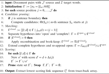
Algorithm 1 processes the source document in a single run over all word positions j, where 1 ≤ j ≤ . It maintains two state lists: the beam of currently active hypotheses or states Γ and the list of newly generated hypotheses Γ′. These will become a future beam in the next round of extension. A search state σ is defined as follows:
 \begin{equation}
\sigma = [\; l\; d ]
\end{equation}
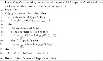
The unified sentence alignment algorithm is a template. Two list processing functions adopt the algorithm to the alignment Types I–III.  (·) specifies how hypotheses are recombined, and
 (·) specifies how a list of hypotheses is extended into new ones. Details are explained in Section 4.

The ‘recombine’ function (·) takes a list of ‘complete’ hypotheses and keeps only the lowest scoring one for all identical states, i.e. for a monotone search we keep the lowest scoring hypothesis for each link end target position i = iend(l). ‘Complete’ states correspond to links whose partial score computation has finished covering all source and target positions for the latest link, i.e. whose link end position equals the current source position j: jend(l) = j. The ‘extension’ function (·) takes a list of recombined hypotheses that correspond to the lowest-scoring partial link sequence ending at a grid-point (j, i) and extends them by a new link l′ covering additional source and target positions, i.e. links for which jbeg(l′) = j+1. The extension function is used to control the links that enter the search space: either sub-sentential or sentence-level links. Similar list-processing functions are used for DP-based SR search (Ney Reference Ney1984) and phrase-based SMT decoding (Och et al. Reference Och2004; Tillmann Reference Tillmann2006) algorithms. An algorithmic definition of the recombination function (·) and the extension function (·) is given in Section 4.1.
Algorithm 1 has three major parts: a candidate pruning step (lines 5–6), a matching step (lines 8–12), and a scoring step (lines 14–17). The candidate pruning step is linked to the extension function (·) in the matching step: the pruning candidate set Θ(S), which is defined in Section 5.1, restricts the possible links that are considered as extensions of a complete partial state. The search starts with a single initial state σ0 in the list Γ (line 2):
 \begin{eqnarray*}
\sigma_0 = [ l_{ini}; 0.0 ]
\end{eqnarray*}
 . It is used to keep track of target sentences that have already been aligned. The use of the target coverage vector is similar to the use of a source word coverage vector in SMT decoders (Koehn, Och and Marcu Reference Koehn, Och and Marcu2003; Och and Ney Reference Och and Ney2004). Here we require that each target sentence is covered at most once (not exactly once), i.e. some target sentences are left uncovered. As target documents may consist of thousands of sentences, the permissible coverage vectors need to be restricted. For each source position j, we compute a restricted target coverage vector: a window of ±10 target positions relative to the so-called coverage focus point is used to compute a restricted coverage vector of length W = 20 (computation of the focus point is explained in Section 5.1).
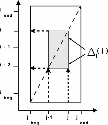
The scoring part of the algorithm is identical for all types of alignments and links. This simplifies the experiments in Section 6. While covering an additional source position j, the target coverage is computed proportionally. Based on the source and target coverage, an incremental matching score Δl(j) = −wT·fj(c = 1, sj, T) is computed (see Figure 4 and (8)). For all search types, the algorithm uses special source null-coverage links for uncovered source chunks. For a monotone search (Type I alignment), target null-coverage links are also needed in order to make sure that a global path that covers an entire document/sentence pair can be computed. Here many-to-many null coverage links are handled as well. The null-coverage score is based on a large null-link constant ϱ(·, ·) = 8.0. Its value is largely compared to the average classifier-based score. As a result, the unified algorithm tries to cover all source and target positions with as few links as possible. Even though the algorithm computes the lowest scoring global link sequence lN 1, each link li is scored separately based on the p(c = 1|S, T) score, e.g. a link l on the global path is only selected if p(c = 1|S, T) > θ, e.g. θ = 0.6. The current two-stack implementation uses only constant memory with respect to the source document length. In comparison, the standard implementation of a full Type I search needs a memory of · . A full Type I sub-sentential fragment monotone search implementation would need · memory. In contrast, the current implementation needs a memory of 2 · and 2 · , respectively (without the candidate pruning).
The partial score computation is based on the link diagonal: the incremental target coverage is computed proportionally to the source coverage. In this example, the link target interval is twice as long as the link source interval. When expanding the source coverage by a single source position j, the partial feature computation is based on the two additional target positions, i−1 and i.

An important component of this memory efficient implementation is the so-called trace-back array. Complete states that pass the recombination step are written into this array. Each state contains the so-called back-pointer, which points to that trace-back array entry (not shown in the state definition in (10)). We can re-cover the partial link sequence corresponding to a state by following the sequence of back-pointers in the trace-back array. The trace-back array is implemented as a linear data structure (Ney Reference Ney1984): A special merge step is used to remove all partial paths that cannot be reached from the states in the set of currently active states Γ. The merge step is important to ensure the constant memory implementation. Once the search is finished, we extract the back-pointer of the lowest scoring state from the final stack at j = . The link sequence is then extracted by running back the trace-back array (line 18). The trace-back array is especially efficient for the Type III search: for each sentence end position at most a single state is written into the trace-back array. Here the trace-back array can be exploited in a novel way to extract an overlapping link sequence. Instead of tracing-back the link sequence of the lowest scoring final state only (this corresponds to the segmentation of source documents into chunks), we extract all the links in the trace-back array, i.e. the lowest scoring link l for each source end position in the document (if it passes the threshold p(l) > θ). Empirically, this improves the utility of the extracted data as shown in Section 6. The handling of overlapping link sequences is similar to the construction of lattice alternatives in SR and statistical MT. The current approach is able to select link alternatives locally that might otherwise not appear in even a large N-best list. In addition, there is only a minimal computational overhead when extracting overlapping links.
4.1 List processing
This section explains how the recombination function (·) and extension function (·) are computed for various alignment and link types. The approach to recombination is explained in detail for the Type I alignment search, where states are defined in (10). We define a lexicographical order on the state set Γ: the states are sorted by the target position i. Within each equivalence class, the hypotheses are then sorted by increasing score. After sorting, states σ that are equivalent to each other, i.e. whose partial link sequences end at the same target position i occur at consecutive array positions. In that list, the lowest scoring states of each such equivalence class occur first. In a single run over the list, whenever we encounter the element of a new equivalence class, we know it is the lowest scoring one, and we just keep this state in the reduced list after recombination. We can formally define the partial hypotheses order as follows:
 \begin{array}{lll}
[i;d]<[i';d'] & {\bf iff} & (i<i')
\end{array}
 \begin{array}{lll}
h' \mbox{eq} h & {\bf iff} & \lnot (h<h') \mbox{and} \lnot (h'<h)
\end{array}
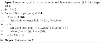
The extension algorithm to compute (·) is illustrated in Algorithm 2. A list of hypotheses Γ is extended by handling each hypothesis σ∈Γ individually and appending the resulting list: (Γ) := ∪σ∈Γ(σ). Algorithm 3 computes an auxiliary function. It generates successor links given the bitext ending position [jend, iend] of the preceding link l. Each state σ∈Γ is extended by L = || possible links, e.g. for a search with the 1-to-4 link set: L = 9 (including null links). For the monotone Type I alignment search, the L successor links start where the previous partial link sequence ends. For the Type II search, new sentence links are generated within a window of W = 20 target sentence positions. At each of these positions, one of the L different links can start. For the Type III alignment search, we search over a large number of candidates: there is no monotone alignment restriction and each of the L alignment types may start at any target sentence position. This search type can only be carried out in connection with the pruning described in Section 5.1, as there might be hundreds of thousands of candidates for a given source sentence. The pruning candidate set is denoted as Θ(Sm), where sm is the m-th sentence in the source document. Here the candidate set Θ(Sm) is computed only once for each sm. The same candidate set pruning is used for the Type I sub-sentential alignment search. Here the length of sub-sentential links is less than ten for both source and target chunks, i.e. the size of the extension set is L = 100. A link l ending at a sentence-internal position is only possible for the sub-sentential search Type I search. These partial sequences are extended monotonically as well. We use the notation l∈Θ to denote a link l whose bitext starting position coincides with the starting position of one of the candidate links. The Type II alignment search extension is handled similarly as the Type III extension and details are given in Section 5.1.
Hypotheses List Extension Function. The function computes the successor states for an hypothesis with link l that ends in bitext position [jend, iend]. The auxiliary function  (·) is defined in Algorithm 3. The link-type set can be defined at run time. λ is a binary variable, where λ = 0 indicates a search for sentence-level and λ=1 for sub-sentential links.

Link extension function (·). The allowable link-type sets are defined in Figure 2. The functions u −1S(j) and u −1T(i) yield the sentence-level position of document word-level source and target position (The indexing functions uS(·) and uT(·) are defined in Section 2.1). As there is no cost for transitions between links, the link score d is just copied into the link extensions.

4.2 Complexity analysis
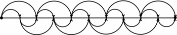
For the Type III alignment search, in analogy to the use of many-to-many links in Type I alignments, we still segment the source document into chunks. There is an exponential number of global paths to be considered as shown in Figure 5. Links that cover neighboring source chunks do not restrict each others' relative target document positions (cf. Figure 3). In particular, we allow the same target chunk to be aligned to several different source chunks ignoring the coverage restrictions of Type I or Type II search. The search is very effective in this case: The list of ‘recombined’ states collapses to just a single active state as the segmentation task focuses on the source chunk segmentation only. A possible disadvantage of the global distance definition as given in (3) is that the global path depends on the path length, and thus shorter paths with fewer links N are favored. Ney (Reference Ney1984) points out a similar disadvantage of a global path length criterion. In the context of sentence alignments, it might lead to locally wrong link boundary decisions. In Section 4, we have presented a simple solution to this problem by allowing links to overlap based on the trace-back array usage. This seems to mitigate the problem in the context of one-to-many links and Type III alignments as shown in Section 6.
Illustration of the number of source document segmentations for a Type III alignment with 2-to-1 links. At each source position two source chunks start (with the exception of path end positions). These are matched against at least a single target chunk and are shown as transition links. Here, there are at least  $2^{({\cal S}-2)/2}$ different segmentation paths where is the number of source sentences.

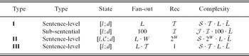
The complexity of different search types is given in Table 1. The corpus parameters , , , and have been defined in Section 2.1. In order to compute the search algorithm complexity for each search type, we count the number of state expansions, i.e. the number of times line 15 in Algorithm 1 is executed. We ignore the complexity for the list processing functions (·) and (·). These operations can be carried out efficiently, whereas the score computation involves expensive probability look-ups based on large data structures. In Table 1, the ‘fan-out’ column gives for each complete search state σ, the maximum number of successor states generated due to the extension function (·). The ‘Rec’ column reports for each search type the maximum number of different hypotheses after the recombination has been carried out for a state list Γ. The complexity given in the last column of Table 1 is derived by multiplying the two preceding ‘fan-out’ and ‘rec’ columns. The factors and take into account that the recombination and extension operations are carried out at sentence boundaries (Types I–III), and possibly all word positions j (Type I sub-sentential alignment). Here,  is the average source chunk length for the L different links. This factor is included as ‘link-internal’ states are extended deterministically in the scoring step in Algorithm 1. For the sub-sentential Type I search, the average source chunk length is = 5 (since the maximum source chunk length is 10). We note that because of the length factor , the complexity is increased more than linearly in the number of link types.
Search complexity for different types along with search state definition, ‘fan-out’ (number of extensions per grid-point), maximum number of hypotheses in the single beam at position j (after recombination), and overall search complexity. is the average number of source words covered by a link. W = 20 is the size of the Type II re-ordering window. The complexity for the sub-sentential search assumes a monotone alignment across the entire document bitext

5 Efficient implementation and pruning
This section presents implementation details that make the sentence-level search efficient. Section 5.1 describes the computation of the beam-search candidate set Θ(S). Section 5.2 presents techniques to efficiently compute the Model-1-based scores in (5) and (6). Finally, Section 5.3 gives details on the computation of the incremental feature vector fj(·) in (8).
5.1 Beam-search pruning
Except for the alignment Type I search, we cannot carry out a full search over the bilingual data. The link sequences lN 1 considered during search must be restricted appropriately. To do so, we modify previous work on extracting one-to-one sentence-level translation pairs from comparable data (Tillmann and Xu Reference Tillmann and Xu2009). During the left-to-right run over the source word-level positions j, whenever we reach the starting position of a sentence S in the source document, we compute the following candidate set of sentence-level 1-to-1-type links li:
 \begin{eqnarray}
\Theta(S) = \{l_i = (S,T_i) |\; T_i\; \mbox{among the lowest scoring}
\;\;\;\;\;\;\;\;\; \mbox{$N$ links with score \varrhov'($S, T_i$)}\; \} \nonumber
\end{eqnarray}
 is the lowest scoring link for the source sentence S, the candidate set contains only those links li for which ρ′(li) ≤ ρ′() + 2.0. The candidate set is also restricted based on the sentence-length ratio introduced by Munteanu and Marcu (Reference Munteanu and Marcu2005): for a sentence pair (S, T) to be considered parallel, the ratio of the lengths of the two sentences has to be smaller than two. In addition, at least half of the words in each sentence have to have a translation in the other sentence based on the Model-1 lexicon and a probability threshold of 5·10−4. For the Arabic–English manually annotated training set used in Section 6, the true translation T for a source sentence S is in Θ(S) for 98 per cent of the source sentences (with all the target sentences Ti as candidates). This candidate set can be computed very efficiently: the early stopping criterion and caching techniques by Tillmann and Xu (Reference Tillmann and Xu2009) are applied appropriately.
For the Type III search, the links considered are restricted based on the candidate set Θ(S) as follows: Only those links l whose bitext start position is identical to one of the links li, i.e. ibeg(l) = ibeg(li) and jbeg(l) = jbeg(li) are considered, i.e. a many-to-many link is considered only if its lower left corner is part of the candidate set. The use of this candidate set in the extension of search hypotheses is shown in Algorithm 2. For the sub-sentential Type I alignment search, the candidate set Θ(S) restricts the number of sub-sentential links that are considered during search: the sub-sentential links l are covered entirely by one of the candidates li, i.e. l⊆li. For the Type II search, we compute the average of all link start positions ibeg(li). This number defines the coverage focus point, which is used to restrict the permissible target coverage vectors in the search states l, ; d. A state σ is extended with links l whose starting position ibeg(l) lies within a window of ±10 positions from that focus point. The target coverage vector ensures that each target sentence is aligned to at most a single source sentence. The candidate pruning step is not applied for the Type I sentence-level search where a full search can be carried out.
The candidate pruning step is related to similar pruning steps in SMT decoders. For a given source segment, i.e. a word or a phrase, only a restricted number of translation candidates are considered in the decoder. Apart from the candidate pruning step, no additional pruning is carried out currently, i.e. there is no global pruning based on the partial scores in the current beam at position j. Due to the candidate set computation, the algorithm's memory usage depends on the average source sentence length in a document. Similar candidate pruning techniques have also been introduced for stack-based DP decoders in SR (Ortmanns, Ney and Eiden Reference Ortmanns, Ney and Eiden1996).
5.2 Efficient lexicalized scoring
In order to make feasible the sentence-level processing pipeline described so-far in this paper, the computation of the Model-1 scoring features in (5) and (6) needs to be very efficient. That efficiency is based on the decomposition of the scoring functions into I+J terms (I τ's and J σ's) where source and target terms are treated differently. While the scoring function computation is symmetrical, the processing is organized according the source language positions. This computational ‘non-symmetry’ is exploited as follows:
• Array access for source term σ(s, T): The computation of the source term σ(s, T) is based on translation probabilities p(s|t). For each source word s, we can retrieve all target words t for which p(s|t) > 0 just once. Those words t along with their probabilities are then stored in an array of the size of the target vocabulary. Words t that do not have an entry in the lexicon have a 0 entry in that array. We keep a separate array for each source position. This way we reduce the probability access to a simple array look-up. Generating the efficient full array data structure requires less than 50 milliseconds per source sentence.
• Caching of target term τ(t, S): For each target word t that occurs in a candidate translation T, the value τ(t, S) can be cached: its value is independent of the other words in T. The same word t in different target sentences is processed with respect to the same source chunk S and τ(t, S) has to be computed only once. Compared with Tillmann and Xu (Reference Tillmann and Xu2009), the cache implementation to account for arbitrary links is extended as follows. We compute the caching function across sentence boundaries and store the following value for each document source position j and target word t:
i.e. we cache a sum of probabilities starting from source position 0. Based on this extended caching function, for any link l, we can compute all the target scores τ(t, S) in the sum σS→T(S, T) in (6) in constant time based on the score difference ct(jend(l))−ct(jbeg(l)). Since a source document may contain hundreds of thousands of words, this caching is carried out on the basis of source language window of 20 sentences. \begin{eqnarray*}
c_t(j)= \sum_{k=0}^j p(t|s_k)
\end{eqnarray*}

The efficient computation of the candidate set Θ(S) also makes use of the caching and array access techniques presented in this section.
5.3 Partial feature vector computation
We select parallel chunk pairs based on the ME classifier defined in (7). It uses the following feature types: coverage, fertility, and intersection. These are computed on the basis of a Model-1 Viterbi alignment where a probability threshold of ε=5·10−4 is used to determine word alignment links. The classifier features are defined such that they can be computed incrementally on a position-by-position basis. To do so, we process the bilingual data one source position at a time. When covering a single source position j, we compute the additional covered target positions incrementally (see Figure 4). Just for this incremental position set, we compute the feature values below: for the single source position, we compute the source lexical, fertility, coverage, and romanization features. For a single target position, we compute target lexical, fertility, and coverage features. If the single source position is mapped to several target positions, their feature values are added. In addition, we compute coverage, length, and intersection features for each source position. Once the algorithm has finished the incremental processing of a given link l, features have been computed that account for exactly |S(l)|+|T(l)| link positions. We use the following eleven features:
Lexical Probability (f1, f2): Two Model-1-based features are derived from the partial sums for the two directions in (5) and (6) : σ(sj, T) and τ(ti, S).
Fertility (f3, f4): We define the fertility of a source word s as the number of target words t∈T for which p(s|t)>ε. A high-fertility word indicates non-parallelism. Target word fertility is defined accordingly.
Consecutive Coverage (f5, f6): A source word s is said to be covered if there is a target word t∈T such that its probability is above a threshold ε:p(s|t)>ε. Consecutive coverage is the number of consecutively covered source word positions to the left of the current source position j. Target coverage is defined accordingly. A long run of covered positions indicates parallelism. In order to compute the coverage features, the search state definition in (10) is modified to keep track of the previous source and target word coverage. In the partial feature vector below, if f 5<3, we use f 5=0 instead. The feature f 6 is handled accordingly.
Coverage (f7): The number of source and target positions covered by the Viterbi path inside a link is used as a feature. High coverage indicates parallelism.
Length (f8, f9): We include the source and target chunk length ratio as ratio ‘penalty’ features: J/I and I/J. These features can be compared to the length penalty in regular SMT decoding (Koehn et al. Reference Koehn, Och and Marcu2003).
Romanization (f10): For each source chunk word s, we compute its Levenshtein distance with respect to all target chunk words ti∈T(l) at the character level. For languages with non-Latin scripts (e.g. Russian and Arabic), the transliteration into Latin is done using an appropriate scheme, e.g. the Buckwalter scheme for Arabic. For the Spanish data, the string itself is used. The transliterated source string s is denoted by tr(s). The following feature value f 10 is computed as
Here, d(t′, ti) is the Levenshtein distance between the transliterated source word t′ and the i-th target word Ti.\begin{eqnarray*}
f_{10} = \left[ 1.0 - \max\limits_{1 \leq i \leq |T|} d(tr(s), t_i) \right]
\end{eqnarray*}Intersection (f11): The intersection feature is defined as the number of alignment points that occur on both Viterbi Model-1 alignments: source to target S→T and target-to-source T→S.

Empirically, we find that normalizing the incremental feature values with respect to source chunk length J or target chunk length I improves classification accuracy. The sentence length normalization has been applied to all the features in our experiments. We define an auxiliary feature vector f j as follows:
 \begin{eqnarray}
\bar{f_j} = (f_1, f_2, f'_3, f_4/I, f'_5, f'_6, f'_7, f'_8, f'_9, f'_{10}, f'_{11})\; \end{eqnarray}
6 Experiments
In this section, we report classification and extraction results for three language pairs: Russian–English, Spanish–English and Arabic–English.
6.1 Data sources and classifier training
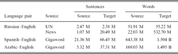
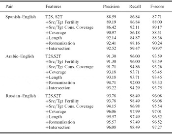
The Russian data come from two sources: United Nations (UN) parallel documents and some news data. The Spanish–English and the Arabic–English data are based on the Gigaword data for these languages (Mendonca, Graff and DiPersio Reference Mendonca, Graff and DiPersio2009; Parker et al. Reference Parker, Graff, Kong, Chen and Maeda2009). The corpus statistics are shown in Table 2. Here, the Russian–English UN data consist of 16, 346 document pairs. For all the languages, the data are tokenized and number-classed (i.e. numbers are replaced with a single tag $num), and the bilingual matching features are computed on this pre-processed data. In addition, if the data does not have sentence-boundary annotation, we use punctuation information to split a text stream into sentences. In Table 3, we present classification results for the ME classifier described in Section 3 in terms of precision, recall, and F-score. The table contains the results for all three language pairs.The size of the annotated data for the Spanish–English, Russian–English, and Arabic–English data is 950, 1, 030, and 1, 600 sentence pairs, respectively. Roughly 80 per cent of the data sets are used to train the classifier and the rest are used for testing. Here the classifier selection threshold θ is set on the training data and lies in a range of [0.6, 0.75] for the different language pairs. The table demonstrates the effect of using different feature sets. The simplest model uses just two lexical probability features, f 1, f 2 from Section 5.3. Each line adds an additional feature, i.e. the final classifier uses all the features, including the Viterbi alignment intersection feature. Including additional features does not always improve classification accuracy. The largest improvements in terms of F-score are reported for the Spanish–English data. In particular, the romanization feature improves accuracy by almost 2 per cent for this European language pair. Another important feature is the intersection feature. For the three language pairs, there is a 0.4 to 0.7 per cent improvement over the classifier results where this feature is not used. For the extraction experiments reported later in this section, we always use the classifier with the full feature set.
Corpus statistics for the three languages pairs on which the extraction algorithm is evaluated

Classifier evaluation in terms of precision/recall/F-score on the manually annotated data for the three languages pairs. The feature functions are defined in Section 5.3

6.2 Translation experiments
We evaluate the performance of the unified search algorithm for different alignment and link types in terms of BLEU (Papineni et al. Reference Papineni, Roukos, Ward and Zhu2002) test set performance. Based on the unified alignment algorithm, chunk pairs are collected from the un-aligned, document-level aligned or comparable data, and this data are added to a baseline system. Using the ME-based extraction algorithm on data with different granularity and types of sentence-level alignments leads to an increased extraction accuracy and/or extraction yield. Only for the Russian–English UN data, there is an alignment at the document level. As the sentence alignment for these document pairs is largely monotone, a search for the alignment Types I and II is used on this data (alignment types have been defined in Section 2). Here, the largest document pair consists of up to 10, 000 source and target sentences. For the Type II alignment search, the beam at a given word position j may contain tens of thousands of states. As the average sentence length is around thirty words for these source sentences, the overall search space reaches billions of states. Processing on such a document pair takes about 1 hour on a single processor. In comparison, for the Russian–English news data, no document boundaries are given and the data can only be processed at the sentence level. For each Russian source sentence, only those target sentences for which the publication date differs less than three days from the publication date of the source sentence, are considered as translation candidates. For the Spanish–English Gigaword data, we also match chunk pairs that have been published from the same news feed, e.g. from a specific news agency like AFP. In addition, the beam-search pruning in Section 5 is used to speed up the search. For this comparable data, even though there is no document alignment, the original sentence order is partially preserved and potentially good many-to-many links can be found. For this data, a sentence-level search for Type III alignments as well as a sub-sentential search for Type I alignments are carried out. Similar experiments are carried out for the comparable English–Spanish and Arabic–English data, which comes from the Gigaword corpora for the years 2003–2008. Again, no document-level alignment is provided for this data. The same three-day publication date filter and sentence-length filter are used. Using a publication date filter of five days increased the number of sentences only slightly.
For the Spanish–English data, already for the one-to-one link search, the search space is huge: link candidates are selected out of 1.08 trillion candidate pairs. There are about 20 million source sentences each of which may have hundreds of thousands of target sentence candidates after the date filter and length filter steps. Since L candidates are considered at each grid point, the overall candidate set of many-to-many links may reach several trillions. Processing the English–Spanish data takes at most two days on a cluster with 300 processors. Processing the Arabic–English data takes less then a single day on the same cluster, while processing the Russian–English UN data takes only a few hours where the un-pruned Type I search runs fastest.
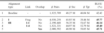
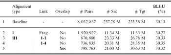
Extraction results are presented for the Russian–English data in Table 4, for the Spanish–English data in Table 5, and for the Arabic–English data in Table 6. The Model-1 probability models used to compute the feature functions in Section 5.3 are trained on the baseline data as well. The Model-1 training has been carried out for two iterations, and the dictionaries are un-pruned and include function words. The Russian–English dictionaries include 97 and 73 million entries, and the Spanish–English dictionaries include 73 and 87 million entries (Source-to-English and English-to-Source, respectively). The use of large un-pruned dictionaries improved extraction recall in preliminary experiments. In the first line of each table we report the number of parallel sentences along with the number of source and target words for the baseline data. On the baseline data, we train a phrase-based system and report its lower cased BLEU score (Papineni et al. Reference Papineni, Roukos, Ward and Zhu2002) on the test sets: for the Russian–English and the Spanish–English data, we use manually collected web news data. The Russian–English data consist of 553 sentences with 20, 602 words and a single reference translation. The Spanish–English data consist of 414 sentences with 13, 474 words and a single reference translation as well. For the Arabic–English data, we use news wire broadcast data collected for the GALE (Olive et al. Reference Olive, Christianson and McCary2011) project. It consists of 683 sentences with 22, 237 words and four reference translations. In terms of parallel data extraction, we have carried out experiments for a combination of different alignment and link types. For each experiment, we report the number of extracted chunk pairs as well as the number of source and target words in the extracted parallel data. The newly extracted data are added to the baseline parallel data (we have not tried to combine the data from different extraction runs). Including the extracted parallel data leads to a significant improvement over the baseline system in all cases. In addition, when searching for Type III sentence-level alignments, we allow many-to-many links to overlap. This novel concept leads to some small improvements in the BLEU score. In Section 4, the use of overlapping link sequences based on the trace-back array has been explained in more detail.
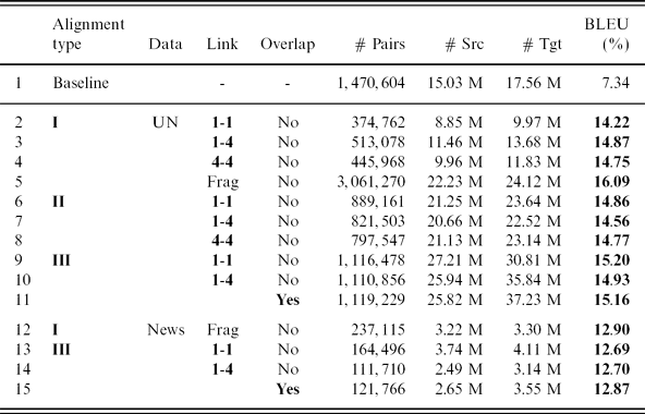
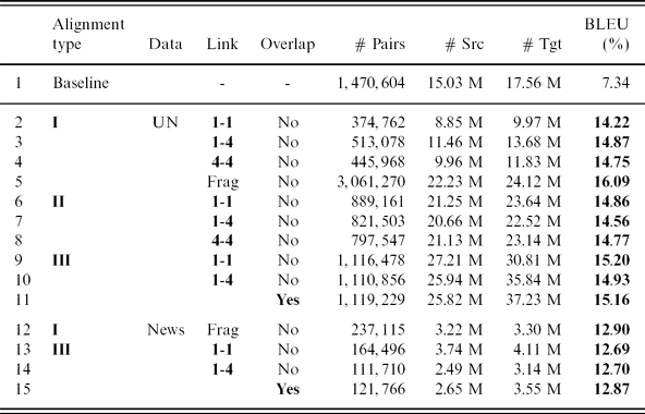
BLEU scores for Russian–English phrase-based SMT systems trained on the baseline data plus some extracted data (UN or news)
BLEU scores for various Spanish–English phrase-based SMT systems trained on the baseline data plus some extracted data (Gigaword)}

BLEU scores for various Arabic–English phrase-based SMT systems trained on the baseline data plus some extracted data (Gigaword)

For the Russian–English results in Table 4, Types I and II alignments are computed for the UN data. Three different link types are extracted: one-to-one, one-to-many, and many-to-many (as shown in Figure 2) where up to four source sentences are aligned to single target sentence and vice versa. Here, the monotone Type I alignment search results are compared with the Type II search results. The Type II search increases the number of chunk pairs significantly. The additional extracted data improve the BLEU score by about 0.6 per cent only for 1-1 link types (line 2 vs. line 6). Even on the largely monotone UN data, the Type III alignment search actually outperforms the monotonic search types: the document pairs are several thousand sentences long, and some sentence re-ordering cannot be handled by the Type II re-ordering window. On this data, the Type I sub-sentential alignment search yields the best BLEU scores (see line 5). For the sub-sentential search, the allowable maximum length ratio has been increased to 4.0 and the coverage threshold has been reduced to 0.33. On the Russian–English news data (results in line 12–15), the sub-sentential search again yields the best extraction results. We carried out pairwise bootstrap re-sampling to determine whether some of the smaller BLEU differences for different search types are statistically significant. The extraction of sub-sentential fragment pairs improved the BLEU score significantly at the 95 per cent level (line 5 vs. line 9 and line 12 vs. line 13). In addition, the extraction of overlapping links improved the BLEU score significantly at the 95 per cent level as well (line 10 vs. line 11 and line 14 vs. line 15). In addition, on the Russian–English news data, we trained an SMT system on the extracted data only. This lead to only a minor drop in translation quality, as the Russian–English test data were taken from the news domain as well.
For the Spanish–English Gigaword experiments in Table 5, the Type III alignment search with 1-1 links performs best (line 3), followed by the sub-sentential search (line 2). Training a phrase-based system on just the extracted data from line 3 leads to lower BLEU performance of 45.45 (down from 46.14). While still yielding a significant BLEU improvement over just using the baseline data, the Type III alignment search with many-to-many links performs worst on this data. Some improvements are obtained by allowing the many-to-many links to overlap (line 4 vs. line 5). In future, we will try to improve translation results by allowing links to overlap for all the link and alignment types, not just the Type III search with many-to-many links. The Arabic–English Gigaword results in Table 6 also show some small improvement over just using the baseline data. Here, already the baseline training data consist of 8 million parallel sentence pairs with more than 200 million words for both source and target language. Consequently, the overall BLEU gains from including the extracted data are small, and the difference between the alignment and link search types are small as well.
7 Comparison and future work
The paper presents a novel one-pass, two-stack beam-search algorithm for extracting parallel text chunk pairs. It unifies several related algorithms into a single framework, and is capable of searching over several trillion link candidates. Here the computation is carried out in parallel over 300 processors. The unified search extends previous work, namely Tillmann (Reference Tillmann2009). In that paper only one-to-one sentence-level links from comparable data are handled, i.e. a special case of the Type III alignment search in this paper. Tillmann (Reference Tillmann2009) presents results that show that avoiding the document-level filtering increases the number of extracted parallel sentence pairs for the Spanish–English Gigaword data. The additional data result in an increased BLEU score as well. The current paper focuses on comparing the effect of different alignment and link types. The beam-search extraction algorithm relies on simple word-based scoring features that can be computed incrementally. In future work, the state definition in (10) can be modified to account for coverage as well as Model-2 or HMM-type distortion model features. In general, the current algorithm is applicable to all extraction methods whose selection features can be computed incrementally. In order to investigate the effect of using incremental features only, the algorithm might also be evaluated in terms of segmentation accuracy on manually annotated data.
It is interesting to compare the size of the extraction classifier search space to the search space that is handled in regular SMT or SR decoding. As is shown in this paper, for a single source sentence the size of the target candidate set might be more than a 100, 000 sentences. In comparison, a SR decoder might have to deal with recognition vocabularies that have up to 100, 000 entries. The number of feature vectors per input pattern is also of the same order of magnitude, i.e. tens of feature vectors. In the current beam-search algorithm, the link-internal matching is deterministic as shown in Figure 4, i.e. this component can not be compared with the word-internal time warping in SR decoders. In future, a ‘fuzzy’ match between source and target sentences could be carried out, e.g. when searching for chunk pairs with gaps. The way the current beam-search decoder computes an alignment score incrementally can be compared with standard phrase-based decoding in SMT. Here, incrementally generated features can obtain close to state-of-the-art performance, which supports their use in this paper. It is also interesting to compare the chunk pair extraction to the extraction of phrase pairs for SMT (Koehn et al. Reference Koehn, Och and Marcu2003). The results in Section 6 show that the lexical Model-1 scoring features defined in Section 3 attain close to the top classification performance. Those lexical scoring features are also commonly used to score phrase pairs in SMT decoding. Likewise, the use of the intersection feature improves classification performance: phrase pairs in SMT are extracted from intersecting word alignments as well. In addition, the paper introduces the following novel concept: In the context of extracting one-to-many sentence pairs on comparable data, the experimental results in Section 6 demonstrate that allowing pairs to overlap in a controlled way actually improves translation results. Again, this method can be related to standard models for phrase-based SMT (Koehn et al. Reference Koehn, Och and Marcu2003; Och et al. Reference Och2004), where the phrase pairs extracted from parallel sentences may overlap based on certain extraction heuristics. In future work, the current chunk-level segmentation algorithm might be improved by allowing overlapping link sequences, in particular when extracting sub-sentential chunk pairs (those could be compared to phrase pairs in SMT with particular long phrases). In addition, the unified algorithm could be extended to search for mixed Types I–III alignment types within a single document pair, which would result in an even more general algorithm.
Similar to Melamed (Reference Melamed1999), the current paper handles the extraction task as a pattern recognition problem. Here our one-pass algorithm is conceptually simpler, since the search in that paper alternates between a generation and a recognition phase. A multi-pass beam-search algorithm (similar to Type I) is presented by Moore (Reference Moore2002). The author uses one-to-one links to bootstrap their lexicon model. Similar bootstrapping techniques might be used in the current work as well. Pike and Melamed (Reference Pike and Melamed2004) present a two-pass algorithm that handles both parallel and comparable data, but it is tested on a small, artificial test set in terms of extraction accuracy. Deng et al. (Reference Deng, Kumar and Byrne2006) describes an approach for segmenting and simultaneously aligning chunks of source and target texts (including sub-sentential chunks). Their paper considers two search strategies: a monotone DP-based search, and an iterative binary search. The iterative binary search is called divisive clustering (DC) search, and it assumes the monotone search as a pre-processing step. It is similar to the Type II search as some non-monotone chunk alignment can be handled. In contrast, the Type II search is based on a coverage vector. Unlike the DC search, it guarantees to find the optimal global segmentation with an appropriately chosen re-ordering window. While Deng et al. (Reference Deng, Kumar and Byrne2006) do not demonstrate any results on comparable data, the current paper focuses on a unified one-stage search algorithm. Brown et al. (Reference Brown, Lai and Mercer1991) also state the use of a constant memory implementation using techniques from Brown et al. (Reference Brown, Spohrer, Hochschild and Baker1982), but no algorithmic details are given. Hewavitharana and Vogel (Reference Hewavitharana and Vogel2011) compare several alignment approaches to extract parallel phrase pairs from sentences that are partially parallel (e.g. sentences marked with red broken lines in Figure 1). In future, we hope that reducing the amount of pre-filtering based on our novel pruning techniques will be especially important for extracting sub-sentential pairs.
8 Acknowledgment
We would like to thank our colleague Young-Suk Lee for suggesting the use of the intersection feature in Section 5.3 and for helpful discussions. We would also like to thank our colleague Yaser Al-Onaizan for his useful comments on our work.