1. Introduction

Bayesian approaches have come to dominate confirmation theory. Most central to these approaches is the concept of probability, typically interpreted subjectively, as indicating a person’s credence (or degree of belief) in a given proposition. Another notion almost as central is that of evidence. We not only believe propositions to differing degrees, but credences can also differ under different suppositions that we might make or can change upon receipt of new information. In the Bayesian paradigm, the notion of evidence has a purely formal definition: E is evidence for H if $p\left(H\right|E)>p(H)$, is evidence against H if $p\left(H\right|E)<p(H)$, and is irrelevant to H if $p\left(H\right|E)=p(H)$, all relative to some person’s credence function p.

There is a third concept, which again builds on the concept of probability, that has not received quite as much attention as probability or evidence but that may have as much theoretical significance as those two. It is what Good (Reference Good1950, Reference Good1983, Reference Good, Bernardo, DeGroot, Lindley and Smith1985) calls the “weight of evidence” and what nowadays is more commonly referred to as the “degree of confirmation.” Good (Reference Good1983, xi) relates that he came to know the notion through his work with Jeffreys and Turing at Bletchley Park and that in his view “it is almost as much an intelligence amplifier as the concept of probability itself.” Psychologists have shown that the notion of degree of confirmation is also deeply rooted in human reasoning, possibly even more deeply than the notion of probability (Tentori, Chater, and Crupi Reference Tentori, Chater and Crupi2016; see also Tentori, Crupi, and Russo Reference Tentori, Crupi and Russo2013).

In the context of developing a new theory of knowledge and building on ideas from Nozick (Reference Nozick1981), Roush (Reference Roush2005, chap. 5) argues that evidence should be a discriminating indicator—it should indicate that a hypothesis is true if it is and only if it is—and that degree of confirmation should measure how well evidence discriminates between a hypothesis being true and its being false. In Roush’s terminology, evidence should track truth, and degree of confirmation should measure how well evidence succeeds in that respect. For Good, Roush, and various other authors (e.g., Eells and Fitelson Reference Eells and Fitelson2002; Hahn, Oaksford, and Bayindir Reference Hahn, Oaksford, Bayindir, Bara, Barsalou and Bucciarelli2005; Fitelson Reference Fitelson2006), the degree to which evidence E confirms hypothesis H is given by the ratio between the likelihoods $p\left(E\right|H)$ and $p\left(E\right|\neg H)$, or at least by a measure ordinally equivalent to it (e.g., one that takes the logarithm of the said ratio). By now, however, many measures of confirmation have been proposed in the literature, besides the aforementioned likelihood ratio measure (see, e.g., Fitelson Reference Fitelson1999; Eells and Fitelson Reference Eells and Fitelson2002; Crupi, Tentori, and Gonzalez Reference Crupi, Tentori and Gonzalez2007; Glass Reference Glass2013).

Authors have been discussing which of those measures is preferable on the basis of vignettes that are supposed to elicit intuitions favoring this measure or militating against that measure. Such vignettes may, for instance, ask readers to imagine a card being drawn from a full deck and then to judge how strongly the finding that the card is a jack confirms the hypothesis that it is a face card (Eells and Fitelson Reference Eells and Fitelson2002). Another approach has been to invoke general principles that supposedly ought to be regarded as general desiderata for measures of confirmation. For instance, Fitelson (Reference Fitelson2006) argues that logicality is one such desideratum, meaning that a measure should reach its maximum when the evidence entails the hypothesis and its minimum when the evidence entails the negation of the hypothesis. Typically, such general principles are also argued for or against by invoking our pretheoretical responses to them.

While this methodological approach is common practice in philosophy, and has also often proved valuable, there are cases in which the back-and-forth between authors appealing to different sets of intuitions has not led to any real progress, let alone to a resolution of a debate. In the debate about measures of confirmation, this methodology may have helped to narrow down the range of plausible candidates, but it has not been able to identify a clear winner. Even if we had strong intuitions favoring a particular measure, one wonders whether the traditional philosophical approach is most appropriate for settling the issue of which measure of confirmation to adopt. If the question is which measure does best at tracking truth, why should we involve our intuitions to begin with? Presumably, the question is empirical: some measures will, as a matter of fact, be better at tracking truth than others. For instance, given two measures of confirmation, a high value of one measure may simply be more frequently associated with the truth of the hypothesis at issue, given the truth of the evidence at issue, than an equally high value of the other measure.

The current article approaches the issue of which measure of confirmation to prefer not quite empirically but quasi-empirically, by turning to computer simulations. The simulations to be presented, while stylized, are realistic enough to offer some insight into the real-world behavior of the various measures of confirmation, specifically, their performance as discriminating indicators. It turns out that some measures do markedly better in this respect than others. If people are sensitive to such differences, then one would expect them to estimate degree of confirmation in a way that is more in accordance with more discriminating measures. This article’s findings will be seen to be in line with empirical results already reported in the literature (Crupi et al. Reference Crupi, Tentori and Gonzalez2007). Indeed, those results are most naturally explained by my findings. The same findings also suggest further empirical work, which could illuminate the question of the broader significance of those findings.

2. Measures of Confirmation

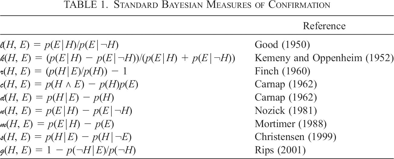
From a Bayesian perspective, it is reasonable to think that the degree to which evidence E confirms hypothesis H must be some function of the credences assigned to E, H, or some of their finite truth-functional combinations. One can construct an almost endless variety of such functions. In practice, only a handful of those have been given serious attention. For many years, philosophers have focused on the measures listed in table 1, which is taken from Crupi et al. (Reference Crupi, Tentori and Gonzalez2007) but extended with the likelihood ratio measure mentioned in the introduction.Footnote ¹

Table 1.

Standard Bayesian Measures of Confirmation

	Reference
𝓁(H, E) = p(E|H)/p(E|¬H)	Good (Reference Good1950)
𝓀(H, E) = (p(E|H) − p(E|¬H))/(p(E|H) + p(E|¬H))	Kemeny and Oppenheim (Reference Kemeny and Oppenheim1952)
𝓇(H, E) = (p(H|E)/p(H)) − 1	Finch (Reference Finch1960)
𝒸(H, E) = p(H ∧ E) − p(H)p(E)	Carnap (Reference Carnap1962)
𝒹(H, E) = p(H|E) − p(H)	Carnap (Reference Carnap1962)
𝓃(H, E) = p(E|H) − p(E|¬H)	Nozick (Reference Nozick1981)
𝓂(H, E) = p(E|H) − p(E)	Mortimer (Reference Mortimer1988)
𝓈(H, E) = p(H|E) − p(H|¬E)	Christensen (Reference Christensen1999)
ℊ(H, E) = 1 − p(¬H|E)/p(¬H)	Rips (Reference Rips2001)

Fitelson (Reference Fitelson1999) was the first to point out that what may appear an embarrassment of riches is in effect just an embarrassment. As he shows, in touting the strengths of Bayesianism, authors have often used the notion of degree of confirmation informally. When their arguments are properly formalized, however, it emerges that they implicitly rely on different measures of confirmation and that an argument that is valid on the assumption of one measure often is not on the assumption of another. While this does not demonstrate that we should come to agree on a unique measure of confirmation, it does show that we should aim to narrow the class of admissible such measures so that we can at least agree on a family of measures that share important characteristics. We can then reevaluate the various arguments for and against Bayesianism in light of the measures that make the cut and see which arguments hold water given any of those measures.

That raises the question of which characteristics measures of confirmation should have. As previously mentioned, Fitelson (Reference Fitelson2006) advocates logicality as one desideratum. This is motivated by the idea that confirmation formalizes a notion of partial entailment, generalizing that of deductive entailment (Kemeny and Oppenheim Reference Kemeny and Oppenheim1952; Carnap Reference Carnap1962). Thus conceived, $E\models H$ and $E\models \neg H$ should emerge as limiting cases on any measure of confirmation, the former constituting the case of maximally strong confirmation of H by E, the latter the case of maximally strong disconfirmation of H by E.

Eells and Fitelson (Reference Eells and Fitelson2002) consider further possible desiderata, focusing especially on symmetries, some of which they regard as desirable properties for a measure of confirmation, others as undesirable properties (see also Fitelson Reference Fitelson2001). For instance, in Eells and Fitelson’s view hypothesis symmetry is a desirable feature, where a measure μ satisfies this feature precisely if $\mu (H,E)=-\mu (\neg H,E)$, for all H, E, and p. By contrast, Eells and Fitelson believe it undesirable for a measure of confirmation to have the property of commutativity symmetry, which holds if and only if (iff) $\mu (H,E)=\mu (E,H)$, for all H, E, and p. They demonstrate that, of the popular measures, 𝒹, 𝓀, and 𝓁 are the only ones to satisfy their desiderata.

Crupi et al. (Reference Crupi, Tentori and Gonzalez2007) propose a more general desideratum, which they state in terms of a function ν that is again fueled by the idea of confirmation as a generalization of entailment. This function is defined as follows: $\nu (H,E)=a$ if $E\models H$, $\nu (H,E)=-a$ if $E\models \neg H$, and $\nu (H,E)=0$ otherwise, given any H and E and with a some positive constant. Crupi et al.’s new desideratum then is that a measure μ should satisfy a symmetry principle σ (such as the principles mentioned in the previous paragraph) in case of confirmation/disconfirmation iff ν satisfies σ in the same case. For example, because $E\models H$ iff $\neg H\models \neg E$, it holds that $\nu (H,E)=\nu (\neg E,\neg H)=a$, regardless of whether E confirms or disconfirms H. It hence follows from Crupi et al.’s desideratum that $\mu (H,E)=\mu (\neg E,\neg H)$ should hold for a measure μ to be acceptable.

One important result reported by Crupi et al. (Reference Crupi, Tentori and Gonzalez2007) is that none of the measures in table 1 satisfies their desideratum. But another is that, from each of those measures, one can easily obtain a measure that does satisfy the desideratum. The trick is to “normalize” the measures via what they reduce to in the limiting cases in which $E\models H$ and $E\models \neg H$. For instance, in the limiting case of confirmation (so if $E\models H$), the measure 𝒹 amounts to $p(\neg H)$, and in the limiting case of disconfirmation (if $E\models \neg H$), 𝒹 amounts to −p(H). These authors then define their new measure 𝓏(H, E) to be $𝒹(H,E)/p(\neg H)$ if $p\left(H\right|E)\ge p(H)$ and $𝒹(H,E)/p\left(H\right)$ otherwise. There is nothing essential to the reference to 𝒹 here; as Crupi et al. show, the parallel construction for any of the other measures yields the same measure 𝓏.

Crupi et al. (Reference Crupi, Tentori and Gonzalez2007) go beyond making a theoretical case for 𝓏. They also present a reanalysis of results of an urn experiment documented in Tentori et al. (Reference Tentori, Crupi, Bonini and Osherson2007). In this reanalysis, they compare 𝓏 and the standard Bayesian measures of confirmation with regard to how strongly predictions based on them correlate with the judgments concerning the impact of new evidence from Tentori et al.’s participants. Tentori and coauthors had found Kemeny and Oppenheim’s (Reference Kemeny and Oppenheim1952) measure 𝓀 to outperform the other standard measures, meaning that the degrees of confirmation predicted by that measure correlated more strongly with registered judgments of confirmational impact than did the degrees of confirmation predicted by any of the other standard measures. However, Crupi et al.’s reanalysis shows that when 𝓏 is included in the comparison, that measure does better still than 𝓀.

Although Crupi and coauthors offer strong theoretical and empirical reasons favoring their 𝓏 measure, these reasons do not entirely clinch the case for that measure (nor do the authors claim otherwise). For one, there is the famous difficulty of arguing from is to ought; for all we know, people’s judgments of evidential impact are subject to a systematic bias, in which case the superiority of 𝓏 in predicting those judgments has little normative significance. For another, the new desideratum Crupi et al. propose, from which the theoretical advantage of 𝓏 is to derive, while not implausible, is also not entirely compelling. Support for it is to come from a vignette involving a rather complicated chance setup about which it is difficult to have strong intuitions. That also explains why later authors have gone on to argue for other measures of confirmation. Most notably, Zalabardo (Reference Zalabardo2009) and Glass and McCartney (Reference Glass and McCartney2015) make different cases for the old likelihood ratio measure, by appeal to different intuitions.

As mentioned in the introduction, though, we are not forced to approach the issue of which measure of confirmation to go with by assessing the various candidates in light of our pretheoretical convictions. For as also mentioned there, Nozick and Roush have proposed to conceive of such measures as instruments for estimating the degree to which evidence succeeds in telling the truth of a hypothesis from its falsity. And conceived that way, these measures are open to empirical scrutiny. Suppose that over a certain period we keep a record of the degrees to which the pieces of information we receive during that period confirm or disconfirm (if either) various hypotheses of interest to us, in which we compute these degrees using all measures of confirmation we deem at least somewhat plausible. At the end of that period, we may not know the truth values of all the hypotheses that were of interest, but we will probably know the truth values of a fair number of them. Insofar as we have registered those truth values, we can check whether, for instance, higher values of a given measure were more strongly associated than lower values with a hypothesis later turning out to be true. More generally, we could ask whether a high degree of confirmation/disconfirmation reliably indicates the truth/falsity of the hypothesis at issue, while less extreme degrees are more weakly associated with truth/falsity. Using standard statistical machinery, we could quantify more finely how accurately degrees of confirmation, given any measure, predict truth values. By doing this for all measures, we could then see which of them is the most discriminating indicator.

While this is straightforward on paper, carrying out this empirical research may be a real challenge in practical terms, if only because our credences are often not accessible to us with a degree of precision that allows us to differentiate among what the confirmational impact of new information is according to different measures of confirmation. To avoid this difficulty, as well as more mundane ones related to consistent bookkeeping, we turn to computer simulations.

3. Tracking Truth

The question before us is which of the measures in the foregoing discussion discriminates most reliably between a hypothesis being true and its being false. All these measures have a “neutral” point, which indicates that the evidence is irrelevant to the hypothesis; a value above that point indicates confirmation, a value below it, disconfirmation.Footnote ² Ideally for these measures, any value above the neutral point indicates truth, and any value below that point indicates falsity, with the indication being stronger, the higher (in the case of truth) or the lower (in the case of falsity) that value is.

Even in this ideal situation, we would not expect all measures to do equally well, qua discriminators. For even then, a high value of μ(H,E) may make it a safer bet to classify H as true if E is known than an equally high value of μ*(H,E), for different measures μ and μ*. And things might not be ideal in the first place: perhaps for a measure μ, values above and below the neutral point are not significantly differently associated with the truth of the hypothesis, meaning that μ would be worthless as a discriminating indicator.

To compare the measures with regard to their discriminatory power, we proceed as follows: $\Omega =\{{\omega }_1,\dots ,{\omega }_n\}$ is a set of possible worlds with a mass function π defined on it, where $\pi \left({\omega }_i\right)>0$ for all i, with $1\le i\le n$ and ${\sum }_i\pi \left({\omega }_i\right)=1$. Propositions are subsets of Ω, and where $1_{\phi }$ is the index set of proposition $\phi \subseteq \Omega$, the probability of φ, p(φ), is given by ${\sum }_{i\in 1_{\phi }}\pi \left({\omega }_i\right)$. Now designate some random world in Ω as the actual one and also randomly pick two propositions from 𝒫(Ω), which we may designate as H and E, making sure only that both are nontrivial (i.e., both are nonempty proper subsets of Ω) and that whichever world we picked as the actual one is a member of E. As the notation suggests, the idea is to interpret H as some hypothesis of interest and E as a potential piece of evidence, where the requirement that the actual world is in E ensures that the evidence is veridical.

Once these choices have been made, we have all the probabilities we need to calculate, for any of our measures, the evidential impact that E has on H, according to the given measure. Furthermore, we can check whether H is true or not: it was picked randomly without any requirement to include the actual world, but of course it may well do so. We can repeat the following steps as often as we like: (i) randomly pick a mass function π on Ω; (ii) pick an actual world, and pick two propositions, subject to the aforementioned requirements; (iii) calculate for each measure the degree to which the proposition that plays the evidence role confirms the proposition that plays the hypothesis role, relative to π; and (iv) register whether the latter is true. The repetitions will output a vector of true/false labels and, for each measure, an associated vector of degrees of support.

What we would like to know, then, is how well the degrees help us to discriminate the labels, that is, how accurately those degrees predict whether the situation was one in which the hypothesis was true or one in which it was false. Given a binary dependent variable (in our case, true/false) and a continuous independent variable (in our case, degree of confirmation), the usual way of determining how helpful the independent variable is for predicting the dependent variable uses the technique of logistic regression. If τ designates the probability that a hypothesis is true, running a logistic regression on data of the kind at issue yields an equation of the form

$\log \frac{\tau }{1-\tau }={\beta }_0+{\beta }_{1}x,$

where x is degree of confirmation (according to a specific measure), and coefficients β₀ and β₁ have been estimated from the data through a maximum likelihood procedure.Footnote ³

Our current interest is not so much in these coefficients but rather in which measure gives rise to the model that best classifies the labels, for that ipso facto answers our question of which measure is the most discriminating indicator. A standard way of evaluating the quality of a logistic regression model, qua binary classifier, is first to convert the output (log odds) to probabilities,Footnote ⁴ next to assume some threshold such that a probability above or equal to that threshold is interpreted as indicating truth and a probability below that threshold is interpreted as indicating falsity, and finally to compare the true positive rate with the false positive rate (i.e., the proportion of true hypotheses correctly identified as such vs. the proportion of false hypotheses incorrectly classified as true). This evaluation makes use of the so-called area under the curve (AUC), which looks at all possible classification thresholds. The AUC value is generally interpreted as a measure of how well a logistic regression model discriminates between the two levels of the dependent variable (see, e.g., Fawcett Reference Fawcett2006).

When we run simulations along these lines, we should reckon with the possibility that the size of Ω matters to how labels relate to degrees. So we should let that size vary within some reasonable range. To model the kind of situation in which we pick two propositions at random, given that these should be nontrivial, we need Ω to have at least four members. In our simulations, we look at numbers of worlds from 5 to 100, in steps of 5. Specifically, for each of those numbers of worlds, we repeat 1,000 times the process of randomly picking an actual world, hypotheses H and E, and weight function π, with each π being drawn anew from the flat Dirichlet distribution for the given number of worlds.Footnote ⁵ We then calculate, for each of those situations and each measure of confirmation, the degree to which E confirms H, and we also register the truth value of H. Next, for each measure of confirmation, we run a logistic regression with registered truth values as the dependent variable and degrees of confirmation (according to the given measure) as the independent variable. And finally we calculate the AUC value of the resulting model. For each number of possible worlds we consider, we repeat these simulations 250 times, to get a sense of the reliability of our results.

Figure 1a shows—for each measure and each number of possible worlds we considered—the AUC score, averaged over the 250 simulations for the given combination. It is immediately evident from that figure that Crupi and colleagues’ 𝓏 measure by far outperforms the competition, at least generally speaking.Footnote ⁶ Even where its performance appears close to Kemeny and Oppenheim’s 𝓀—namely, for 5 worlds—a two-sided t-test conducted on the results of the 250 simulations for that measure and 𝓏 shows that the latter does reliably better, at a level of $\alpha <.0001$; t-tests for the other numbers of worlds came out significant at the same α level.Footnote ⁷

Figure 1.

Mean AUC values of the various measures obtained in simulations for possible worlds from 5 to 100, increasing in steps of 5. a, Simulations in which each world had the same chance of being selected as the actual world; b, simulations in which each world’s chance of being selected as the actual world was equal to the probability mass attributed to it in the simulation.

In the above simulations, each $\omega \in \Omega$ had the same probability $1/\left|\Omega \right|$ of being actual. A variant of these simulations well worth considering lets the probability with which a world ω is picked to be actual in a given simulation depend on the probability mass that is assigned to ω at the start of that simulation. The variant makes particularly good sense if we think of π as determining the objective probability with which the various worlds in Ω are actual and think of our credences as tracking those objective probabilities.Footnote ⁸

Keeping everything else the same, we obtain the results shown in figure 1b. While the picture is a bit more complicated now, it is still the case, from 25 worlds onward, that 𝓏 outperforms the other measures (at $\alpha <.0001$); for 5, 10, and 15 worlds, 𝓀 does slightly although significantly ($\alpha <.0001$) better; and for 5 worlds, 𝓃 does a little better as well, and also significantly so ($\alpha <.0001$).Footnote ⁹

Depending on which of the two sets of simulations we look at, 𝓏 is either always or for the most part a significantly more discriminating indicator than the other measures. While that is an important finding in itself, it also helps to explain what had remained something of a mystery in Crupi et al. (Reference Crupi, Tentori and Gonzalez2007). For, why does 𝓏 predict the judgments gathered for the experiment from Tentori et al. (Reference Tentori, Crupi, Bonini and Osherson2007) more accurately than the other measures? It is difficult to imagine that ordinary people are sensitive to the feature that 𝓏 respects certain supposedly desirable symmetries but violates certain supposedly undesirable ones. None of those symmetries strikes one intuitively as being either so compelling or so misguided that that would be a plausible assumption. Yet, if the notion of evidential impact is psychologically salient in the way some research suggests, then it is imaginable how, through use and trial and error, people have come to implicitly prefer to measure that impact in a way that makes the result as discriminating as possible or at least as discriminating as they could figure out how to make it. In this connection, it is further noteworthy that 𝓀, which came out second best in the empirical part of Crupi et al. (Reference Crupi, Tentori and Gonzalez2007), also emerges as a clear second in our simulations.

4. Can We Do Better?

The methodology applied in the previous section offers a different approach to the question of which measure of confirmation is preferable, an approach that does away with previous reliance on case-based intuitions and that gives full weight to the practical significance of measuring evidential impact. As mentioned, only a handful of all possible functions that we can build from probabilities assigned to a hypothesis H, evidence E, and their finite truth-functional combinations have been probed as measures of confirmation. Among those never seriously considered, there might well be hiding some with greater discriminatory power than 𝓏. Given the sheer number of candidates, however, systematically searching the solution space seems out of reach here. In this kind of case, looking at variants of solutions already known to do well is often a good idea.

Fitelson and Hitchcock (Reference Fitelson, Hitchcock, Illari and Russo2011) point at the closeness between the discussion concerning measures of confirmation and that concerning measures of causal strength. For instance, Lewis (Reference Lewis1986) proposes what is in effect 𝓁 as a measure of causal strength. And the measure 𝓈, which Christensen (Reference Christensen1999) proposes as a measure of confirmation, has also been doing duty as a measure of causal strength in the literature on causality, where it mostly goes by the name of “Δp rule” (Shanks Reference Shanks1995). In her influential paper, Cheng (Reference Cheng1997) argues that this rule is inferior to what she dubs the “power PC [probabilistic contrast] account.”

To my knowledge, the power PC account has not yet been considered as possibly contributing to confirmation theory, but it might be worth doing so, given that, formally, this measure is a relatively minor variant of Crupi et al.’s 𝓏 measure. Using the measure 𝓈 where Cheng uses Δp, her measure of the generative power of E for H is defined to be

$𝒽(H,E)≔\{\begin{array}{cc}\frac{𝓈(H,E)}{p(\neg H|\neg E)}& \text{if}𝓈(H,E)\ge 0\\ \frac{𝓈(H,E)}{p\left(H\right|\neg E)}& \text{otherwise.}\end{array}$

When $𝓈(H,E)<0$, Cheng prefers to speak of the preventive power, or inhibitory power, of E for H and, therefore, takes the negative of the second clause as stated here, but that is just a semantic issue.

In section 2, we defined 𝓏 in terms of 𝒹 but also noted that the former can be defined just as well in terms of any of the other measures in table 1. To facilitate comparison with Cheng’s measure, we restate it here in terms of Christensen’s measure:Footnote ¹⁰

$𝓏(H,E)≔\{\begin{array}{cc}\frac{𝓈(H,E)}{p(\neg H)/p(\neg E)}& \text{if}𝓈(H,E)\ge 0\\ \frac{𝓈(H,E)}{p\left(H\right)/p(\neg E)}& \text{otherwise.}\end{array}$

This makes it easy to see that the only differences between 𝓏 and Cheng’s measure reside in the denominators in both clauses.

Superficially at least, the difference between the measures appears to be small. Is it of any theoretical significance? Crupi and colleagues’ decision to divide by $p(\neg H)/p(\neg E)$ and $p\left(H\right)/p(\neg E)$ in the first and second clauses, respectively, is motivated by their wish to obtain a measure with range [−1 ,1] that reaches its maximum if $E\models H$ and its minimum if $E\models \neg H$ (see also Crupi and Tentori Reference Crupi and Tentori2013). It takes little effort to show that 𝒸𝒽 satisfies not only this condition but also the various constraints that follow from Crupi et al.’s (Reference Crupi, Tentori and Gonzalez2007) main desideratum (see sec. 2 above), an overview of which is provided by table 3 in their paper.

To see that 𝒸𝒽 has the same range as 𝓏, it suffices to note that 𝒸𝒽 can be rewritten as

$\frac{p\left(H\right|E)-p(H|\neg E)}{1-p\left(H\right|\neg E)},$

for the case in which $𝓈(H,E)\ge 0$, and as

$-\frac{p\left(H\right|\neg E)-p(H\left|E\right)}{p\left(H\right|\neg E)},$

for the alternative case. (Note also that $p\left(H\right|\neg E)>p(H\left|E\right)$ in the latter case.)

As for the other conditions, first consider the case in which $𝓈(H,E)\ge 0$. Then we have that

$𝓏(H,E)=\frac{p(\neg E)}{p(\neg H)}\times 𝓈(H,E)$

and also that

$𝒸𝒽(H,E)=\frac{p(\neg E)}{p(\neg H\wedge \neg E)}\times 𝓈(H,E),$

or equivalently

$𝒸𝒽(H,E)=\frac{p(\neg E)}{p(\neg H)p(\neg E|\neg H)}\times 𝓈(H,E),$

or again

$𝒸𝒽(H,E)=\frac{1}{p(\neg E|\neg H)}\times \frac{p(\neg E)}{p(\neg H)}\times 𝓈(H,E),$

or finally

$𝒸𝒽(H,E)=\frac{1}{p(\neg E|\neg H)}\times 𝓏(H,E).$

By parallel reasoning, we find that if $𝓈(H,E)<0$, then 𝒸𝒽(H, E) can be rewritten as $1/p(\neg E|H)\times 𝓏(H,E)$.

From this, it follows that if $E\models H$, then $𝒸𝒽(H,E)=𝓏(H,E)$, given that then $\neg H\models \neg E$ and so $1/p(\neg E|\neg H)=1$; it similarly follows that $𝒸𝒽(H,E)=𝓏(H,E)$ if $E\models \neg H$. It further follows that there is a piecewise-defined function f such that $𝒸𝒽(H,E)=f\left(𝓏\right(H,E\left)\right)$, where f is injective and $f\left(x\right)=-f(-x)$. Because it also holds that $𝒸𝒽(H,E)>/=/<0$ if $p\left(H\right|E)>/=/<p(H)$, all conditions of lemma 3 in Crupi et al. (Reference Crupi, Tentori and Gonzalez2007, 249) are fulfilled for 𝒸𝒽 to enjoy all consequences of the new desideratum proposed by these authors.

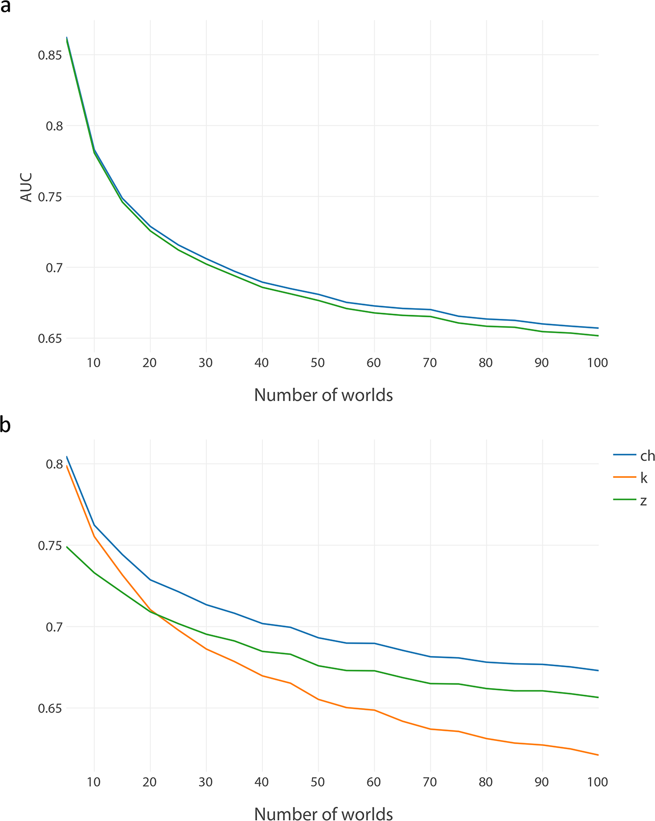
The discussion above also makes it easy to see that, in general, $𝒸𝒽(H,E)>𝓏(H,E)$ if $𝓈(H,E)\ge 0$, and $𝒸𝒽(H,E)<𝓏(H,E)$ if $𝓈(H,E)<0$. Might this at least be of practical significance, even if theoretically the two measures are close cousins? To find out, we apply the methodology from the previous section and rerun the same simulations, now just focusing on 𝓏 and the new measure 𝒸𝒽 in the simulations in which all worlds have the same chance of being actual and on 𝓏, 𝒸𝒽, and 𝓀 in the simulations in which a world’s probability mass determined its chance of being actual. (Here 𝓀 is taken into account as well because it sometimes performed best in the corresponding simulations above.) The results of these simulations are shown in figure 2. We see that, in the first set of simulations, the new measure improves at least a little over 𝓏. The t-tests on the AUC values for the measures show that while the differences between the means are not significant for 5 and 10 worlds, they are from there on: from 15 to 65 worlds at an α level of .05, and above 65 worlds at an α level of .005.Footnote ¹¹ In the second set of simulations, the new measure improves a lot over 𝓏, with all t-tests being significant at $\alpha <.0001$. The new measure also does consistently better than 𝓀, and even for 5 and 10 worlds, where the two are relatively close, the difference is significant at $\alpha =.0001$.Footnote ¹²

Figure 2.

Mean AUC values for 𝒸𝒽 and 𝓏 (a) and 𝒸𝒽, 𝓀, and 𝓏 (b) obtained in simulations for possible worlds from 5 to 100, increasing in steps of 5. a, Simulations in which all worlds had an equal chance of being selected as the actual world; b, simulations in which each world’s chance of being selected as the actual world equaled its probability mass in the simulation.

Admittedly, these are just the outcomes of simulations, and it is another question whether the difference between the measures is big enough to matter in people’s reasoning. One way to check would be by reusing the data set that Crupi and colleagues used to compare the measures discussed in their paper. We might find that 𝒸𝒽 predicts human judgments of evidential impact more accurately than 𝓏. Better still, one could run new experiments more specifically designed to differentiate between 𝓏 and 𝒸𝒽. I am, in fact, hoping that the results reported here will inspire psychologists to undertake this work. For now, I hope to have shown that the new methodology may be fruitfully deployed in a quest for measures of confirmation that are possibly more discriminating than the ones we already have.

5. Conclusion

We started from Roush’s observations that we want our evidence to reliably discriminate between truth and falsity and that a measure of confirmation should quantify how successful a piece of evidence is in this regard. These observations inspired an approach to assessing measures of confirmation that circumvents questions of how intuitively compelling this or that condition is as a desideratum for such measures. Applying the approach to the most prominent measures of confirmation led to the finding that Crupi et al.’s (Reference Crupi, Tentori and Gonzalez2007) measure 𝓏, which already enjoyed considerable backing—theoretical as well as empirical—also outstrips the competition in power to discriminate between truth and falsity. As we saw, however, there is no reason why we should leave matters there. We already discovered one measure that does at least somewhat better than the one proposed by Crupi and colleagues. Others may be out there, possibly some that do quite a bit better. The methodology put forward in this article is easy to implement and thereby facilitates the identification of such measures.