

1 Introduction
A large body of recent research in political science has been devoted to identifying and explaining ideological polarization, especially, but not only in the United States. There is strong evidence that the U.S. Congress has grown progressively more polarized since the 1970s (McCarty, Poole, and Rosenthal Reference McCarty, Poole and Rosenthal2006), as well as some evidence of a polarization trend in presidential platforms (Budge et al. Reference Budge, Klingemann, Volkens, Bara and Tanenbaum2001; Klingemann et al. Reference Klingemann, Volkens, Bara, Budge and McDonald2006). Many empirical studies link this increasing ideological divide between the main American parties to legislative gridlock, elite incivility, income inequality, and voter disengagement (Hetherington Reference Hetherington2001; Layman and Carsey Reference Layman and Carsey2002; Fiorina and Abrams Reference Fiorina and Abrams2008). Across a broader range of countries, polarization is associated with democratic breakdown, corruption, and economic decline (Linz and Stepan Reference Linz and Stepan1978; Frye Reference Frye2002; Brown, Touchton, and Whitford Reference Brown, Touchton and Whitford2011). To complement these empirical findings, many existing models of electoral competition and policymaking show that parties with conflictual preferences are socially suboptimal (Persson and Svensson Reference Persson and Svensson1989; Alesina and Tabellini Reference Alesina and Tabellini1990; Azzimonti Reference Azzimonti2011). However, as we hope to show, these conclusions depend crucially on a number of stylized assumptions about the nature of the disagreement among political actors. While we lack a precise notion of ideological polarization when parties care about multiple dimensions, how we measure this concept crucially affects the conclusions on its welfare consequences.
In this article, we develop a model designed to study the policy consequences of ideological conflict when political actors have preferences over public policies on two separate issues.Footnote 1 We highlight that—when parties and voters care about multiple issues—we can use many different measures to describe the degree of conflict—or polarization—among agents’ preferences in the political arena, and we propose two such measures. The first measure, which we label extremism, is the ideological distance of each party from the decisive voter in the electorate. The second measure, which we call antagonism, is the ideological distance that separates the two parties from each other and summarizes the degree of political competition between policymakers. These two measures coincide in a one-dimensional policy space, where the ideological distance between the two parties can increase only as they move further away from the representative voter.Footnote 2 However, they do not coincide in a two-dimensional setting: here, the two parties can be very close (when they share views on both dimensions) or very different (when they are perfectly opposed in one dimension), without altering their overall distance from the representative voter.
In our model, parties run in the many elections of an infinite horizon and commit to enact the same policy for their entire tenure in office. This incumbent policy persistence reflects politicians’ inability to credibly promise policies different than those implemented while in office. This constraint is well documented and arises for many concurring reasons: internal party politics which generates organizational hysteresis (Miller and Schofield Reference Miller and Schofield2003); voters’ focus on parties’ records and neglect of novel campaign promises (retrospective voting, Fiorina Reference Fiorina1981); the electoral costs of changing policy position and being perceived as flip-floppers (Adams et al. Reference Adams, Clark, Ezrow and Glasgow2006; Tavits Reference Tavits2007; Tomz and Van Houweling Reference Tomz and Van Houweling2008, Reference Tomz and Van Houweling2012; DeBacker Reference DeBacker2015). Not all parties face the same constraints, though. Following an electoral defeat, parties usually replace their leaders. This, together with the fact that their past policy platform has not been enacted and observed by voters, means that challengers are better able to credibly change their policy stance.Footnote 3 We assume that incumbents who remain in office find it too costly to implement policies that differ from those of their previous term. In particular, we model two parties who compete in an election in each of an infinite number of periods; the opposition party proposes a policy platform while the incumbent party, if reelected, enacts the same policy from the previous period. A representative voter picks her favorite candidate. The election winner implements the proposed policy and commits to do so for the duration of its tenure. In this sense, the identity of the incumbent party and its policy represent a dynamic linkage across periods.
There are two main questions that we wish to address with this simple setting. First, what is the impact of ideological disagreement on implemented policies when parties are long-lived and care about present as well as future electoral outcomes? Second, how do electoral competition, ideological disagreement and parties’ dynamic incentives affect the electorate’s welfare?
We fully characterize a Stationary Markov Perfect Equilibrium (SMPE) of the dynamic electoral competition described above and prove it exists for any discount factor, any initial incumbent’s policy, and any degree of antagonism and extremism.Footnote 4 According to the results of our model, parties alternate in power and long-run policies tends to be more moderate, in the sense of being closer to the preferences of the representative voter: (i) the larger is the degree of antagonism between alternating governments; (ii) the smaller is parties’ extremism; (iii) the larger is parties’ patience. Opposition parties’ ability to design a winning policy around the incumbents’ commitment drives alternation in power. The key idea behind moderation is that an opposition party—which knows it is tying its hands with the current policy platform and, hence, will be vulnerable to future electoral defeat—has incentives to behave strategically by offering policies that restrict the set of policies future challengers can win an election with. In particular, the opposition party restricts the future challenger by contesting the election with a platform closer to the median voter’s ideal policy: winning with a more moderate platform today makes the median voter more demanding in the following election. The more the preferences of the challenger depart from the preferences of the current government, that is, the higher antagonism is, the more the challenger will try to restrict the future opposition’s ability to win an election with a platform close to its ideal policy. On the other hand, the degree of conflict between the parties and the representative voter, that is, extremism, does not affect the strategic incentives to moderate: increasing extremism increases both the marginal benefit of moderation (that is, the gain from constraining the future incumbent to more moderate policies) and its marginal cost (that is, the loss from implementing policies further away from the bliss point), leaving their ratio constant. As a consequence, a more extreme party will generally offer a more extreme policy platform.
This analysis suggests that the influence voters exert on policies is a function of the degree of antagonism and extremism of the political system. In particular, polarization can have counter-intuitive welfare implications: the electorate is best served by highly antagonist political elites that are perfectly opposed on one dimension.
2 Related Literature
This paper contributes primarily to the theoretical literature on the relationship between political elites’ polarization and policy outcomes. In a multidimensional and static framework, Krasa and Polborn (Reference Krasa and Polborn2014) study how ideological polarization on one dimension influences the candidates’ positions on a second dimension. In most dynamic models, conflictual political preferences are socially suboptimal (Persson and Svensson Reference Persson and Svensson1989; Alesina and Tabellini Reference Alesina and Tabellini1990; Azzimonti Reference Azzimonti2011; Prato Reference Prato2016). Our paper shares with this literature the idea that forward-looking incumbents have incentives to strategically position current policies to affect future political outcomes, and that these incentives are stronger when the conflict of preferences is starker. On the other hand, in our model disagreement can be over multiple dimensions and the channel to constrain a future incumbent is the demands of the electorate rather than inefficient or misdirected spending. Our novel approach shows that—when the ideological conflict is multidimensional—preference divergence does not necessarily lead to higher inefficiencies and welfare losses for the electorate, but it could have the opposite effect.
More recent studies argued that polarized parties and divergent platforms can be welfare enhancing (Bernhardt, Duggan, and Squintani Reference Bernhardt, Duggan and Squintani2009; Bernhardt et al. Reference Bernhardt, Campuzano, Squintani and Camara2009; Van Weelden Reference Van Weelden2013, Reference Van Weelden2015). In these works, polarization coincides with our notion of extremism and helps the electorate through channels different than the one highlighted in our paper. Van Weelden (Reference Van Weelden2013, Reference Van Weelden2015) shows that, in a more polarized political environment, the incumbent gives up rent extraction for fear of being replaced by a challenger with markedly different policy preferences. Bernhardt, Duggan, and Squintani (Reference Bernhardt, Duggan and Squintani2009) analyze a static and unidimensional electoral competition where more polarized parties propose more extreme electoral platforms; for moderate levels of polarization, this is welfare enhancing because it provides the median voter with a more varied choice. Bernhardt et al. (Reference Bernhardt, Campuzano, Squintani and Camara2009) study repeated elections where candidates’ types are private information and show that the incumbent will compromise more if his potential replacement is drawn from the other side of the political spectrum. In our case, on the other hand, the beneficial effect of antagonism comes from more moderate policies implemented strategically by forward-looking incumbents of known type, and increased extremism is always detrimental to the representative voter.
Our work is related to a growing theoretical literature on dynamic elections with endogenous economic or political state variables (Krusell and Rios-Rull Reference Krusell and Rios-Rull1999; Bai and Lagunoff Reference Bai and Lagunoff2011; Battaglini Reference Battaglini2014). The key assumption in our model, namely, the differential ability of incumbents and challengers to adjust policy platforms, owes to the seminal work of Kramer (Reference Kramer1977) and Wittman (Reference Wittman1977), who pioneered the study of dynamic models of asynchronous policy competition. While Kramer (Reference Kramer1977) and Wittman (Reference Wittman1977) focus on myopic parties, Forand (Reference Forand2014) considers farsighted parties who take into account future opponents’ policy choices and offer policy platforms on a single dimension. With a single dimension, the ideological distance between the two parties coincide with the disagreement between the parties and the median voter. In this framework, the incentive to moderate in order to constrain future incumbents exists but it is unchanged as we increase the ideological distance between the two parties. To the contrary, the parties and voters in our setup care about multiple dimensions. Expanding the policy space beyond a single dimension allows us to explore the different facets of ideological polarization and to highlight the ambiguous impact of parties’ conflict of preferences on the electorates’ welfare.Footnote 5
Less closely related to this paper is the literature on dynamic elections with adverse selection and/or moral hazard (for example Duggan Reference Duggan2000; Bernhardt, Dubey, and Hughson Reference Bernhardt, Dubey and Hughson2004; Banks and Duggan Reference Banks and Duggan2009; Kalandrakis Reference Kalandrakis2009, see Duggan and Martinelli Reference Duggan and Martinelli2015 for comprehensive survey). This literature stresses the link between parties’ policies and their reelection prospects and, typically, features some degree of incumbency advantage due to the electorate’s greater information on the incumbent. In our model, instead, the incumbent’s commitment to a policy and the lack of any uncertainty generate deterministic alternation in power. Therefore, the policy platform chosen by the challenger in a given election only affects the policy with which her opponent will defeat her in the next election.
Finally, our paper is also formally related to models of dynamic legislative bargaining with an endogenous status quo and farsighted players (Baron Reference Baron1996; Kalandrakis Reference Kalandrakis2004; Diermeier and Fong Reference Diermeier and Fong2011; Bowen, Chen, and Eraslan Reference Bowen, Chen and Eraslan2014; Dziuda and Loeper Reference Dziuda and Loeper2016). To view our model as a legislative bargaining model, reinterpret the representative voter as the median legislator, the parties as the only legislators that have the power to set the agendaFootnote 6 , and define the state variable as the status quo policy, that is, the policy implemented by the legislature in the previous period.
3 Model and Equilibrium Notion
We describe here a dynamic model of electoral competition between policy and office motivated parties. In each period of an infinite horizon, two parties,
 $1$
and
 $2$
, compete in an election decided by a representative voter
 $v$
. Each period starts with a party as the incumbent office holder and the other party, the opposition, striving to replace it in power. A key feature of our model is incumbent policy persistence: incumbents cannot distance themselves from their past policies, while opposition parties can put forward new policies more freely.
The electoral process
Elections occur at the beginning of each period. The opposition party contests an election by offering a bidimensional policy
 $\mathbf{p}=(p^{1},p^{2})\in X=\mathbb{R}^{2}$
, or stays out of the race. The incumbent party is committed to the policy
 $\mathbf{q}\in X$
that brought it into office. The representative voterFootnote
7
is, thus, confronted with the choice between
 $\mathbf{p}$
, promised by the opposition party, and
 $\mathbf{q}$
, the continuing policy of the incumbent party. The elected party implements its winning policy and becomes the incumbent at the beginning of the next period. The policy implemented in a period becomes the incumbent’s policy commitment in the next period and, as such, represents a dynamic linkage between periods.
Stage utilities
The stage utility player
 $i\in \{1,2,v\}$
receives from policy
 $\mathbf{p}\in X$
is measured by the squared distance of
 $\mathbf{p}$
from
 $i$
’s bliss point, or ideal policy,
 $\mathbf{b}_{i}=(b_{i}^{1},b_{i}^{2})$
:
 $$\begin{eqnarray}u_{i}(\mathbf{p})=-(p^{1}-b_{i}^{1})^{2}-(p^{2}-b_{i}^{2})^{2}.\end{eqnarray}$$
Denoting by
 $d(\mathbf{x},\mathbf{y})$
the usual Euclidean distance between
 $\mathbf{x}\in X$
and
 $\mathbf{y}\in X$
, we can rewrite equation (1) as
 $u_{i}(\mathbf{p})=-d^{2}(\mathbf{p},\mathbf{b}_{i})$
.Footnote
8
We abuse notation slightly and denote by
 $d(\mathbf{x})=||\mathbf{x}||$
the distance from the origin of
 $\mathbf{x}\in X$
. In addition to policy, parties care about being in office. The party in power in a period receives office rents
 $r\geqslant \bar{r}$
, where
 $\bar{r}$
is determined and its role is discussed in the equilibrium analysis below. Office-holding benefits include patronage positions in government and government-owned companies, public financing of party activities and other office perks that are consumed only by the party in government. The utility
 $i$
derives from a sequence of policies
 $\mathbf{P}=\{\mathbf{p}_{0},\mathbf{p}_{1},\ldots \}$
is the discounted sum of payoffs from each period:
 $$\begin{eqnarray}U_{i}(\mathbf{P})=\mathop{\sum }_{t=0}^{\infty }\unicode[STIX]{x1D6FF}_{i}^{t}\left[u_{i}(\mathbf{p}_{t})+\mathbb{I}_{i,t}\cdot r\right]\end{eqnarray}$$
where
 $\unicode[STIX]{x1D6FF}_{i}\in [0,1)$
is player
 $i$
’s discount factor and
 $\mathbb{I}_{i,t}=1$
when party
 $i$
is in power in period
 $t$
and zero otherwise. The representative voter receives no utility from
 $r$
, hence
 $\mathbb{I}_{v,t}=0$
for any
 $t$
. We assume
 $\unicode[STIX]{x1D6FF}_{1}=\unicode[STIX]{x1D6FF}_{2}\equiv \unicode[STIX]{x1D6FF}$
and
 $\unicode[STIX]{x1D6FF}_{v}=0$
.Footnote
9
Parties’ antagonism and extremism
The model is shift and rotation invariant, so, without loss of generality, we define the representative voter’s bliss point as the origin of the plane,
 $\mathbf{b}_{v}=(0,0)$
, party 1’s bliss point as
 $\mathbf{b}_{1}=(b_{1},0)$
and party 2’s bliss point as
 $\mathbf{b}_{2}=(b_{2}^{1},b_{2}^{2})$
with
 $d(\mathbf{b}_{2})=b_{2}$
. The distance of the bliss point of party
 $i\in \{1,2\}$
from the bliss point of the representative voter is
 $b_{i}$
. The parameter
 $b_{i}$
, thus, captures the ideological distance between the voter and the party. We call this the degree of extremism of party
 $i$
.
A second, separate, measure of ideological divergence is given by the angle
 $\unicode[STIX]{x1D6FC}\in [0,\unicode[STIX]{x1D70B}]$
formed by the two vectors
 $\mathbf{b}_{1}$
and
 $\mathbf{b}_{2}$
.Footnote
10
This parameter captures how different the parties’ bliss points are from each other, regardless of their distance from the representative voter’s ideal policy. When
 $\unicode[STIX]{x1D6FC}=0$
, the parties’ bliss points are on the same ray departing from the origin. When
 $\unicode[STIX]{x1D6FC}\in (0,\unicode[STIX]{x1D70B})$
, the two parties diverge on both dimensions, keeping the distance from the origin of the plane constant. When
 $\unicode[STIX]{x1D6FC}=\unicode[STIX]{x1D70B}$
, the two parties are perfectly opposed on one dimension and share the same ideology on the second dimension. We call
 $\unicode[STIX]{x1D6FC}$
the degree of antagonism of the parties.
While we define antagonism and extremism using a two-dimensional policy space,
 $X$
, our definitions and results would be identical in a similar model with more than two dimensions. In particular, the equilibrium characterized in Proposition 1 survives in a model with
 $X=\mathbb{R}^{n}$
. In this model, the definitions of antagonism and extremism, as well as the equilibrium strategies, will take place on the two-dimensional hyperplane in
 $\mathbb{R}^{n}$
that contains the bliss points of the parties and of the representative voter.
The equilibrium strategies we characterize below depend solely on the distance between the incumbent’s policy and the bliss point of the representative voter, that is, the origin of the plane. We denote with
 $k_{i}(\mathbf{x})=\frac{d(\mathbf{x})}{b_{i}}\geqslant 0$
for
 $i\in \{1,2\}$
the distance of policy
 $\mathbf{x}\in X$
from the origin, relative to
 $b_{i}$
. With this notation,
 $k_{i}(\mathbf{q})\mathbf{b}_{i}$
is a point on the line connecting
 $\mathbf{b}_{v}$
with
 $\mathbf{b}_{i}$
, at the same distance from
 $\mathbf{b}_{v}$
as the incumbent’s policy commitment
 $\mathbf{q}$
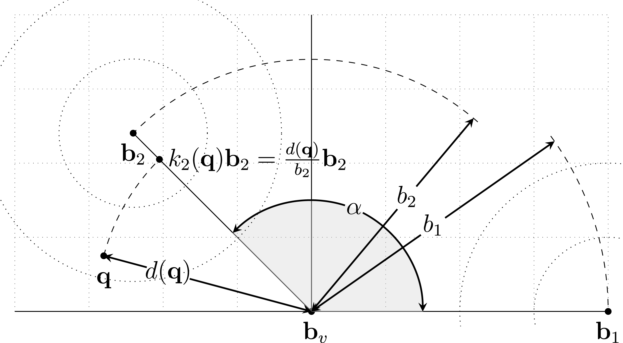
. Figure 1 shows the basic model parameters: a set of arbitrary bliss points for the three players (
 $\mathbf{b}_{v}$
,
 $\mathbf{b}_{1}$
, and
 $\mathbf{b}_{2}$
) and the indifference curves generated by their Euclidean preferences over policies; the corresponding degree of antagonism (
 $\unicode[STIX]{x1D6FC}$
) and extremism (
 $b_{1}$
,
 $b_{2}$
); the incumbent’s policy commitment (
 $\mathbf{q}$
) and its distance from the origin (
 $d(\mathbf{q})$
); and a point on the line connecting
 $\mathbf{b}_{2}$
with the origin, at the same distance from the origin as the incumbent’s policy (
 $k_{2}(\mathbf{q})\mathbf{b}_{2}$
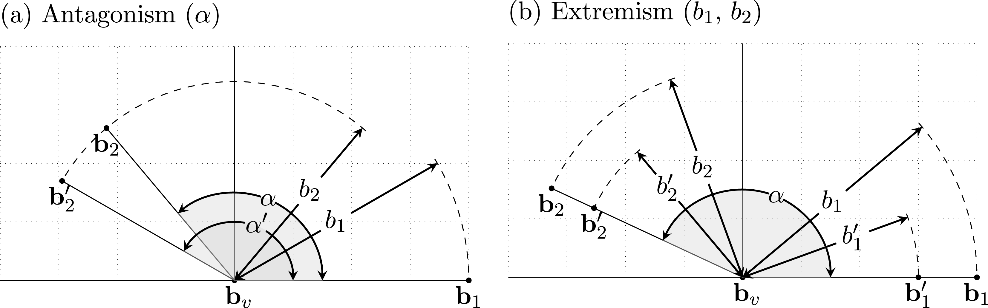
). Figure 2 shows examples of parties’ bliss points for two different degrees of antagonism (
 $\unicode[STIX]{x1D6FC}^{\prime }>\unicode[STIX]{x1D6FC}$
) and two different degrees of extremism (
 $b_{i}^{\prime }>b_{i}$
).
Basic Model Parameters.

Parties Bliss Points for Different Levels of Antagonism and Extremism.

Strategies
We focus on equilibria in pure Markov strategies (Maskin and Tirole Reference Maskin and Tirole2001). We assume that the decision of the opposition party regarding which policy to run with, should it contest the election, depends solely on the incumbent’s identity and the policy it is committed to. Markovian strategies that abstract from the history of play are standard in dynamic models of political economy (Baron Reference Baron1996; Kalandrakis Reference Kalandrakis2004, Reference Kalandrakis2010; Battaglini, Nunnari, and Palfrey Reference Battaglini, Nunnari and Palfrey2012; Duggan and Kalandrakis Reference Duggan and Kalandrakis2012; Duggan and Forand Reference Duggan and Forand2013; Forand Reference Forand2014), capture the simplest form of behavior consistent with rationality, and clearly isolate the underlying strategic motives shaping the competition between the two parties in a dynamic environment, independent of the time horizon. In addition, the two parties interact over a long time horizon and can be represented by different politicians in different points in time. Therefore, strategies that potentially depend on events from the (distant) past and require coordination might be excessively demanding and inappropriate for the context at hand. Given the policies of the two parties in a contested election, we assume the representative voter elects the party running with the policy she prefers and votes for the opposition when indifferent.Footnote 11
Definition 1. A Stationary Markov strategy for the opposition party
 $i\in \{1,2\}$
, given incumbent
 $j=\{1,2\}\setminus \{i\}$
, is a function
 $\unicode[STIX]{x1D70E}_{i}:\{j\}\times X\rightarrow X\cup \{Out\}$
, mapping
 $j$
’s policy commitment
 $\mathbf{q}\in X$
into an electoral platform
 $\mathbf{p}\in X$
or the decision not to contest the election (‘Out’). A Stationary Markov strategy for the representative voter
 $v$
is a function
 $\unicode[STIX]{x1D70E}_{v}:(\{1,2\}\times X)\times X\rightarrow \{\text{Yes},\text{No}\}$
that maps
 $j$
’s policy commitment
 $\mathbf{q}\in X$
and the electoral platform of the opposition
 $\mathbf{p}\in X$
into the decision to elect the opposition.
Dynamic utilities
We denote by
 $V_{i}^{j}(\mathbf{q}|\unicode[STIX]{x1D70E})$
the dynamic utility party
 $i\in \{1,2\}$
derives from the infinite sequence of policies generated by the profile of strategies
 $\unicode[STIX]{x1D70E}=(\unicode[STIX]{x1D70E}_{1},\unicode[STIX]{x1D70E}_{2},\unicode[STIX]{x1D70E}_{v})$
, at the beginning of a period with incumbent party
 $j\in \{1,2\}$
committed to
 $\mathbf{q}$
. Formally, if
 $\mathbf{P}(\,j,\unicode[STIX]{x1D70E},\mathbf{q})=\{\mathbf{p}_{0},\mathbf{p}_{1},\ldots \}$
is a path of policies generated by play according to
 $\unicode[STIX]{x1D70E}$
, starting from an incumbent
 $j$
committed to
 $\mathbf{q}$
, we have:
 $$\begin{eqnarray}V_{i}^{j}(\mathbf{q}|\unicode[STIX]{x1D70E})=U_{i}(\mathbf{P}(\,j,\unicode[STIX]{x1D70E},\mathbf{q}))=\mathop{\sum }_{t=0}^{\infty }\unicode[STIX]{x1D6FF}^{t}\left[u_{i}(\mathbf{p}_{t})+\mathbb{I}_{i,t}\cdot r\right].\end{eqnarray}$$
Equilibrium notion
We look for a stationary Markov perfect equilibrium.
Definition 2. A Stationary Markov Perfect Equilibrium (SMPE) is a profile of Stationary Markov strategies
 $\unicode[STIX]{x1D70E}^{\ast }=(\unicode[STIX]{x1D70E}_{1}^{\ast },\unicode[STIX]{x1D70E}_{2}^{\ast },\unicode[STIX]{x1D70E}_{v}^{\ast })$
such that, for any
 $\mathbf{q}\in X$
,
 $$\begin{eqnarray}\unicode[STIX]{x1D70E}_{i}^{\ast }\in \{_{\unicode[STIX]{x1D70E}_{i}}\,V_{i}^{j}(\mathbf{q}|(\unicode[STIX]{x1D70E}_{i},\unicode[STIX]{x1D70E}_{j}^{\ast },\unicode[STIX]{x1D70E}_{v}^{\ast }))\end{eqnarray}$$
for any
 $i\in \{1,2\}$
and
 $j=\{1,2\}\setminus \{i\}$
, and
 $\unicode[STIX]{x1D70E}_{v}^{\ast }(\,j,\mathbf{q},\mathbf{p})=\text{Yes}$
if and only if
 $$\begin{eqnarray}u_{v}(\mathbf{p})\geqslant u_{v}(\mathbf{q}).\end{eqnarray}$$
An equilibrium, as specified in (5), requires that the representative voter supports the opposition if and only if her expected utility from the incumbent’s policy is not larger than the expected utility from the opposition’s platform. The fact that the opposition optimizes its dynamic utility is ensured by (4).
4 Equilibrium Analysis
4.1 Simple strategies
In the remainder, we focus on a class of SMPE of the dynamic electoral competition game, where the two parties use strategies of a simple form, captured by a single parameter
 $\hat{k}_{i}$
.
Definition 3. A Simple (Stationary Markov) strategy
 $\unicode[STIX]{x1D70E}_{i}$
for
 $i\in \{1,2\}$
, satisfies
 $$\begin{eqnarray}\unicode[STIX]{x1D70E}_{i}(\mathbf{q})\equiv \mathbf{p}_{i}(\mathbf{q})=\left\{\begin{array}{@{}ll@{}}k_{i}(\mathbf{q})\mathbf{b}_{i}\quad & \text{for }k_{i}(\mathbf{q})\leqslant \hat{k}_{i}\\ \hat{k}_{i}\mathbf{b}_{i}\quad & \text{for }k_{i}(\mathbf{q})\geqslant \hat{k}_{i}\end{array}\right.\end{eqnarray}$$
where
 $\hat{k}_{i}$
is a parameter. A Simple Stationary Markov Perfect Equilibrium (SSMPE) is an SMPE where the parties use simple strategies.Footnote
12
As discussed above,
 $k_{i}(\mathbf{q})$
measures the distance of the incumbent’s policy commitment
 $\mathbf{q}$
from the origin of the plane. According to these simple strategies, when
 $\mathbf{q}$
is closer than
 $\hat{k}_{i}$
to the origin, the opposition party
 $i\in \{1,2\}$
contests the election with
 $k_{i}(\mathbf{q})\mathbf{b}_{i}$
. This policy is located on the ray that connects
 $\mathbf{b}_{v}$
with
 $\mathbf{b}_{i}$
, and it is at the same distance from
 $\mathbf{b}_{v}$
as the incumbent’s policy commitment
 $\mathbf{q}$
. When, instead,
 $\mathbf{q}$
is further than
 $\hat{k}_{i}$
from the origin, the opposition party
 $i\in \{1,2\}$
runs with
 $\hat{k}_{i}\mathbf{b}_{i}$
. This policy is on the same ray that connects
 $\mathbf{b}_{v}$
with
 $\mathbf{b}_{i}$
, but it is
 $\hat{k}_{i}$
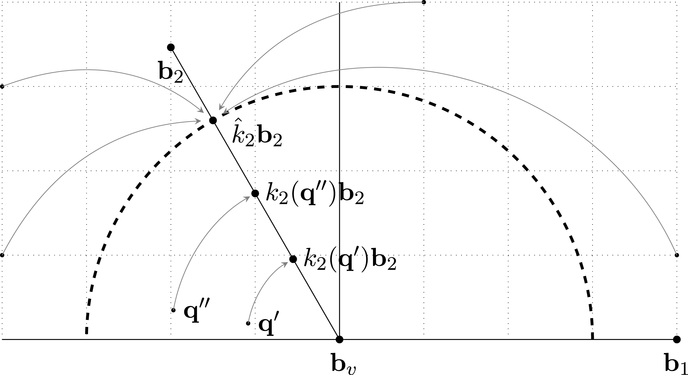
distant from the origin. Figure 3 shows the policies corresponding to these simple strategies: for a number of arbitrary party 1’s policy commitments, the arrow indicates the policy platform chosen by party 2. Consider how the policies evolve as
 $k_{2}(\mathbf{q})=\frac{d(\mathbf{q})}{b_{2}}$
increases, that is, as party 1’s policy commitment moves further away from the origin: for low values of
 $k_{2}(\mathbf{q})$
, the policy
 $\mathbf{p}_{2}(\mathbf{q})$
increases linearly—that is, it gets further away from the origin—as
 $k_{2}(\mathbf{q})$
increases; once
 $k_{2}(\mathbf{q})$
reaches
 $\hat{k}_{2}$
,
 $\mathbf{p}_{2}(\mathbf{q})$
stays constant and it is not affected by a further increase of
 $k_{2}(\mathbf{q})$
.
Simple Stationary Markov Proposal Strategy.

4.2 Results
Proposition 1 below shows that an SSMPE of the dynamic electoral competition game exists and is generally unique, and it fully characterizes it.
Proposition 1 (SSMPE of Dynamic Electoral Competition Game).
Assume, without loss of generality, that
 $b_{1}\geqslant b_{2}$
. Then:
1.
 $\hat{k}_{1}=1$
and
$\hat{k}_{2}=\frac{1+\unicode[STIX]{x1D6FF}\cos \unicode[STIX]{x1D6FC}}{1+\unicode[STIX]{x1D6FF}}$
characterize a SSMPE;
2. if
$b_{1}>b_{2}$
, this SSMPE is unique; if
$b_{1}=b_{2}$
, there exists exactly one additional ‘mirror’ SSMPE where
$\hat{k}_{1}$
and
$\hat{k}_{2}$
are reversed;3. in any SSMPE, elections are contested and incumbents always defeated;
4. starting from
$\mathbf{q}^{0}$
, SSMPE policies converge to alternation between(a)
$k_{1}(\hat{k}_{2}\mathbf{b}_{2})\mathbf{b}_{1}$
and
$\hat{k}_{2}\mathbf{b}_{2}$
, if
$k_{2}(\mathbf{q}^{0})\geqslant \hat{k}_{2}$
,(b)
$k_{1}(\mathbf{q}^{0})\mathbf{b}_{1}$
and
$k_{2}(\mathbf{q}^{0})\mathbf{b}_{2}$
, if
$k_{2}(\mathbf{q}^{0})\leqslant \hat{k}_{2}$
.


Proof. See Appendix A.☐
In a SSMPE, the policy platforms chosen by party
 $i\in \{1,2\}$
always lie on the ray starting at
 $\mathbf{b}_{v}$
, the origin of the plane, and passing through
 $\mathbf{b}_{i}$
, its ideal policy. We call such a ray a
 $\mathbf{b}_{i}$
-ray. To understand why, consider the dynamic utility
 $i$
derives from running with a policy
 $\mathbf{p}$
the representative voter prefers to
 $\mathbf{q}$
:
 $u_{i}(\mathbf{p})+r+\unicode[STIX]{x1D6FF}V_{i}^{i}(\mathbf{p}|\unicode[STIX]{x1D70E})$
. In this expression, the first two terms capture the current utility following an electoral victory. The third term captures the future stream of payoffs, given the policy commitment. This discounted value depends on
 $d(\mathbf{p})$
but not on the specific location of
 $\mathbf{p}$
: the strategies of all players depend on the distance of the incumbent’s policy commitment from the origin, but not on its exact location. As a result, when moving
 $\mathbf{p}$
along any circle centered at
 $\mathbf{b}_{v}$
, the dynamic utility of
 $i$
increases as
 $\mathbf{p}$
approaches the
 $\mathbf{b}_{i}$
-ray. This increases the utility accrued in the current period but maintains constant the future utility.
Strategic Incentives in SSMPE.

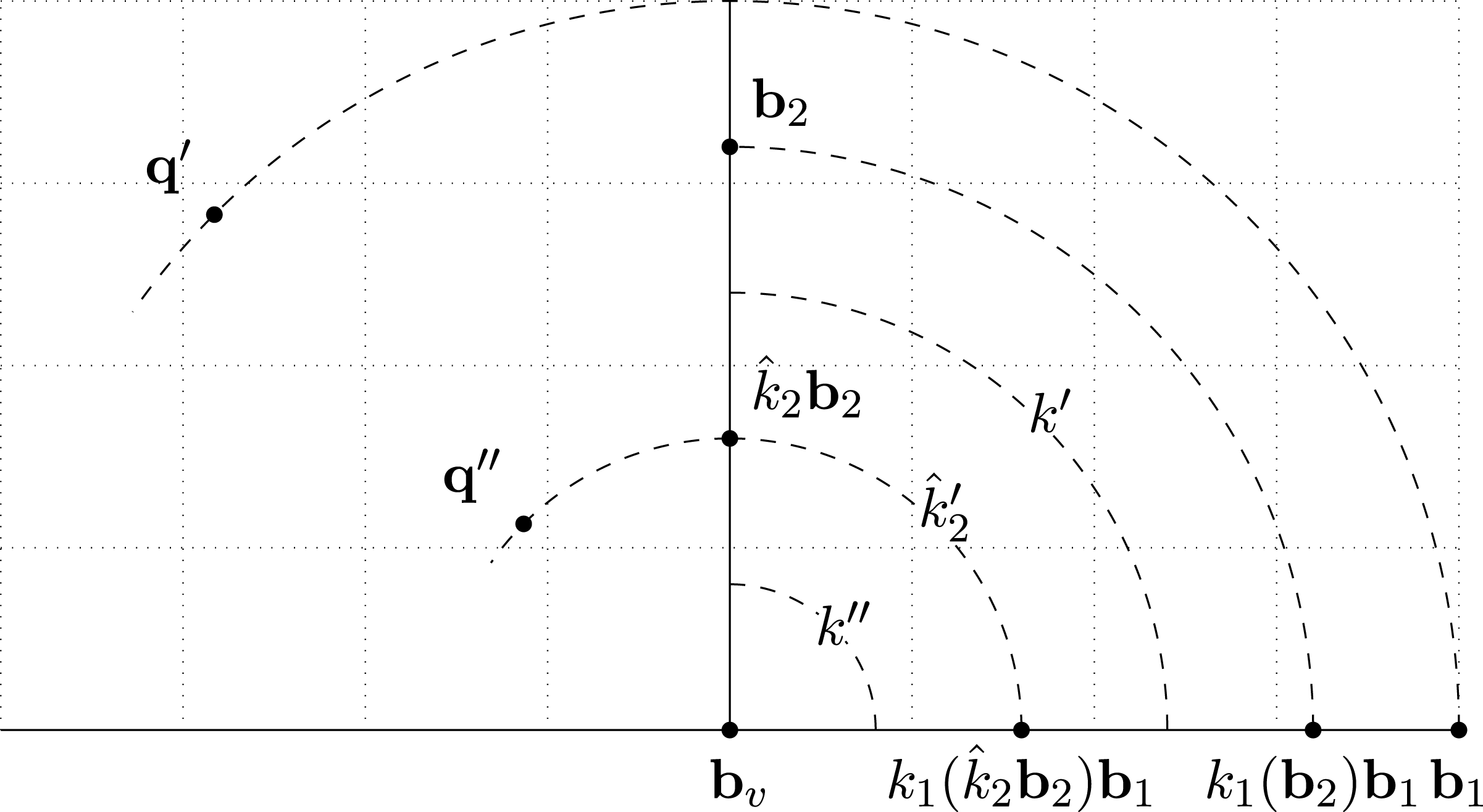
Figure 4 shows many different circles centered at
 $\mathbf{b}_{v}$
, in dashed lines. These circles represent the indifference curves of the representative voter. For a given incumbent’s policy commitment,
 $\mathbf{q}$
, the representative voter elects the challenger if it proposes any policy at least as close to her bliss point, that is, on the boundary or strictly inside the corresponding indifference curve. For the parties, the simple strategies from Proposition 1 prescribe that party
 $2$
runs with
 $\hat{k}_{2}\mathbf{b}_{2}$
for any incumbent’s policy commitment
 $\mathbf{q}$
with
 $d(\mathbf{q})\geqslant d(\mathbf{q}^{\prime \prime })$
and runs with
 $k_{2}(\mathbf{q})\mathbf{b}_{2}$
for any
 $\mathbf{q}$
with
 $d(\mathbf{q})\leqslant d(\mathbf{q}^{\prime \prime })$
. Similarly, party
 $1$
runs with
 $\hat{k}_{1}\mathbf{b}_{1}=\mathbf{b}_{1}$
or
 $k_{1}(\mathbf{q})\mathbf{b}_{1}$
depending on whether
 $d(\mathbf{q})\gtrless d(\mathbf{q}^{\prime })$
.
We first discuss the intuition underlying the strategy of party 2. When
 $d(\mathbf{q})\leqslant d(\mathbf{q}^{\prime \prime })$
, running with
 $k_{2}(\mathbf{q})\mathbf{b}_{2}$
means running with a policy on the
 $\mathbf{b}_{2}$
-ray with the same distance from the origin as
 $\mathbf{q}$
. For incumbent’s policy commitments close to the origin, party
 $2$
is constrained by the demand of the representative voter and runs with a winning platform as close as possible to its bliss point
 $\mathbf{b}_{2}$
. On the other hand, when
 $d(\mathbf{q})\geqslant d(\mathbf{q}^{\prime \prime })$
, party
 $2$
runs with
 $\hat{k}_{2}\mathbf{b}_{2}$
, a policy strictly inside the voter’s acceptance set. Consider, for example, an incumbent party
 $1$
committed to
 $\mathbf{q}^{\prime }$
from Figure 4. In this case, the voter is willing to elect a challenger party
 $2$
that runs with its bliss point,
 $\mathbf{b}_{2}$
, because this policy is closer to the voters’ bliss point than
 $\mathbf{q}^{\prime }$
. A perfectly myopic opposition would propose this policy platform. However, a forward-looking opposition finds it optimal to run with policy
 $\hat{k}_{2}\mathbf{b}_{2}$
, which is closer to
 $\mathbf{b}_{v}$
than
 $\mathbf{b}_{2}$
. We call this behavior moderation.
The incentive to moderate is purely strategic and arises from the dynamic nature of the game. On the one hand, moderating has a cost: running with
 $\hat{k}_{2}\mathbf{b}_{2}$
, rather than
 $\mathbf{b}_{2}$
, harms party
 $2$
in the current period, since the policy it implements when in office is further away from its bliss point. On the other hand, moderating has a benefit: winning the current election with a more moderate policy helps in the following period; party
 $2$
will be committed to a more moderate platform and this makes the representative voter more demanding. If party
 $1$
wants to regain power, it is forced to propose
 $k_{1}(\hat{k}_{2}\mathbf{b}_{2})\mathbf{b}_{1}$
, a policy that both the representative voter and party
 $2$
prefer to
 $k_{1}(\mathbf{b}_{2})\mathbf{b}_{1}$
(what party
 $1$
would propose with an incumbent committed to
 $\mathbf{b}_{2}$
). The extent of moderation,
 $\hat{k}_{2}$
, is then determined by the strength of two forces. The first force pushes the opposition’s policy in the direction of its bliss point, in an attempt to increase its current utility. The second, strategic force, pushes the opposition’s policy in the direction of the representative voters’ bliss point, in an attempt to constrain the future behavior of the defeated incumbent. As we discuss in the following section, the magnitude of this latter force depends on the parties’ patience and on the intensity of their ideological disagreement. The equilibrium extent of moderation is the value of
 $\hat{k}_{2}$
that balances the marginal static cost with the marginal dynamic benefit.
We now discuss the equilibrium strategy of party
 $1$
. Contrary to party
 $2$
, party
 $1$
does not moderate: it proposes its ideal policy
 $\mathbf{b}_{1}$
whenever the representative voter prefers it to the incumbent’s commitment. Why is this the case? While the two parties have similar strategic incentives to moderate, moderation is a strategic substitute. Assume party
 $1$
moderates, that is, it proposes a policy closer to the origin than
 $\mathbf{b}_{1}$
. This has a cost in the current period: all moderate policies reduce its current utility from holding office. On the other hand, since party
 $2$
already moderates, not all moderate policies give a benefit in the following period, in terms of leading to future policies closer to its ideal point. Party
 $1$
will affect the electoral strategy of its challenger only if it moderates to
 $k_{1}(\hat{k}_{2}\mathbf{b}_{2})\mathbf{b}_{1}$
or to a policy even closer to the origin, for example, referring again to Figure 4, to
 $k^{\prime \prime }\mathbf{b}_{1}$
. Moderating less—that is, running with
 $k^{\prime }\mathbf{b}_{1}$
or any other policy between
 $\mathbf{b}_{1}$
and
 $k_{1}(\hat{k}_{2}\mathbf{b}_{2})\mathbf{b}_{1}$
—will not make any difference in the following election, as party
 $2$
will run with
 $\hat{k}_{2}\mathbf{b}_{2}$
as prescribed by its moderating strategy. However, moderating to
 $k_{1}(\hat{k}_{2}\mathbf{b}_{2})\mathbf{b}_{1}$
or more is too costly in terms of foregone current utility and party
 $1$
abandons the idea of moderation altogether. This explains why an equilibrium in simple strategies must be asymmetric, with one party moderating and the other one sticking to its guns. The reason why party
 $2$
is the one who moderates lies in the fact that party
 $1$
has a weaker incentive to moderate: its ideal policy is more extreme and, thus, the future utility gain it gets from constraining its opponent is smaller.Footnote
13
The assumed lower bound on office rents,
 $\bar{r}\equiv \max \{b_{1},b_{2}\}^{2}(1+\unicode[STIX]{x1D6FF})$
, guarantees that, in equilibrium, both parties find it advantageous to contest elections rather than staying out of the race and leaving the incumbent indefinitely in power. To understand why, consider the case where party
 $1$
is the incumbent and is committed to enact policy
 $\mathbf{q}$
. Absent any office motivation, the opposition party can ensure a payoff of
 $\frac{u_{2}(\mathbf{q})}{1-\unicode[STIX]{x1D6FF}}\leqslant 0$
by never running for office. For party 2 to voluntarily contest an election for any state
 $\mathbf{q}\in X$
, the optimal policy characterized in Proposition 1 must give her at least what she can get by running with
 $\mathbf{b}_{v}$
, the bliss point of the representative voter. This policy platform ensures electoral victory for any
 $\mathbf{q}$
and gives party
 $2$
a payoff of
 $\frac{u_{2}(\mathbf{b}_{v})}{1-\unicode[STIX]{x1D6FF}}+\frac{r}{1-\unicode[STIX]{x1D6FF}^{2}}$
. While sufficiently large office rents are necessary to construct an SSMPE, their magnitude has no effect on the equilibrium policy platforms. This apparently surprising result is due to the lack of electoral uncertainty in our model: the opposition party which decides to contest an election either wins or loses for sure. In a similar model with a nondegenerate reelection probability, increasing office rents would weaken policy motivation; since a weaker policy motivation affects both the costs and benefits of moderation, increasing office rents would have an uncertain effect on the parties’ incentive to moderate in equilibrium.
Long-Run policies and convergence dynamics
Proposition 1 also specifies the long-run policies that we converge to as a consequence of equilibrium strategies. We have three cases to consider. First, assume the initial incumbent’s policy commitment,
 $\mathbf{q}^{0}$
, is at least as close to the origin as the strategically induced bliss point of party 2,
 $\hat{k}_{2}\mathbf{b}_{2}$
. In this case, the representative voter’s acceptance set is binding in all elections and all policies will lie at the same distance from the origin as the initial incumbent’s policy commitment. The policies implemented will alternate between
 $k_{2}(\mathbf{q}^{0})\mathbf{b}_{2}$
and
 $k_{1}(\mathbf{q}^{0})\mathbf{b}_{1}$
, depending on the identity of the incumbent.
Second, assume the initial incumbent’s policy commitment is further away from the origin than
 $\mathbf{b}_{1}$
. If party
 $1$
is at the opposition in the first period, it wins the election with its ideal policy
 $\mathbf{b}_{1}$
. In the second period, party
 $2$
wins the election with
 $\hat{k}_{2}\mathbf{b}_{2}$
, a policy the representative voter strictly prefers to the incumbent’s policy commitment
 $\mathbf{b}_{1}$
. In all future periods, the policy implemented will be at the same distance from the origin, alternating between
 $\hat{k}_{2}\mathbf{b}_{2}$
, when
 $2$
is in power, and
 $k_{1}(\hat{k}_{2}\mathbf{b}_{2})\mathbf{b}_{1}$
, when
 $1$
is in power. If party
 $2$
is at the opposition in the first period, it wins the election with
 $\hat{k}_{2}\mathbf{b}_{2}$
and the policy dynamic immediately reaches alternation between
 $\hat{k}_{2}\mathbf{b}_{2}$
and
 $k_{1}(\hat{k}_{2}\mathbf{b}_{2})\mathbf{b}_{1}$
.
Finally, assume
 $\mathbf{q}^{0}$
is further away from the origin than
 $\hat{k}_{2}\mathbf{b}_{2}$
but closer to the origin than
 $\mathbf{b}_{1}$
. This case is similar to the second one, except that, if party
 $1$
is at the opposition in the initial period, it is constrained to offer
 $k_{1}(\mathbf{q}^{0})\mathbf{b}_{1}$
. From the second period, we have the same alternation between
 $\hat{k}_{2}\mathbf{b}_{2}$
and
 $k_{1}(\hat{k}_{2}\mathbf{b}_{2})\mathbf{b}_{1}$
.
5 Representative Voter’s Welfare
The welfare of the representative voter from an ex ante perspective, that is, at the beginning of the game, depends on the identity of the incumbent and on its policy commitment in the first period. Instead of making arbitrary assumptions, we assume that party
 $1$
is the first-period incumbent with probability
 $\unicode[STIX]{x1D70C}\in (0,1)$
and that its policy commitment
 $\mathbf{q}^{0}$
is distributed according to a continuous cumulative distribution function
 $F(\mathbf{q}^{0})$
with strictly positive density on
 $X$
.
Definition 4. In the SSMPE from Proposition 1, the ex ante welfare of
 $v$
is:
 $$\begin{eqnarray}W(\hat{k}_{1},\hat{k}_{2},b_{1},b_{2})=\int _{X}\unicode[STIX]{x1D70C}u_{v}(\mathbf{p}_{2}(\mathbf{z}))+(1-\unicode[STIX]{x1D70C})u_{v}(\mathbf{p}_{1}(\mathbf{z}))\,d(F(\mathbf{z})).\end{eqnarray}$$
Lemma 1 shows that the representative voter is strictly worse off as the degree of policy moderation observed in equilibrium decreases and as the parties bliss points diverge from the representative voter’s bliss point.
Lemma 1. In the SSMPE from Proposition 1, the ex ante welfare of the representative voter is decreasing in
 $\hat{k}_{2}$
,
 $b_{1}$
, and
 $b_{2}$
.
Proof. See Appendix A.☐
6 Comparative Statics
The following proposition formalizes the marginal impact of the model parameters on the strategic force pushing the parties toward moderation:
Proposition 2 (SSMPE Comparative Static).
In the SSMPE from Proposition 1:
 $$\begin{eqnarray}\frac{\unicode[STIX]{x2202}\hat{k}_{2}}{\unicode[STIX]{x2202}\unicode[STIX]{x1D6FC}}\leqslant 0\quad \frac{\unicode[STIX]{x2202}\hat{k}_{2}}{\unicode[STIX]{x2202}\unicode[STIX]{x1D6FF}}\leqslant 0.\end{eqnarray}$$
Proof. Immediate.☐
 $\hat{k}_{2}\mathbf{b}_{2}$
as a function of
 $\unicode[STIX]{x1D6FC}$
and
 $b_{2}$
 $\unicode[STIX]{x1D6FF}\rightarrow 1$
and
 $b_{1}>b_{2}$
.

Proposition 2 says that the strategic force pushing the more moderate party toward moderation gains strength as the ideological conflict between the parties becomes more pronounced (higher
 $\unicode[STIX]{x1D6FC}$
) and as the future becomes more important (higher
 $\unicode[STIX]{x1D6FF}$
). As discussed in the previous section, parties have an incentive to moderate because they internalize that, if they locate closer to the median, then the rival will have to, as well. When parties are more patient, they care relatively more about what the rival will do next period, so the more moderate party will locate closer to the representative voter to induce the rival to do the same. The same occurs when ideological divergence rises: for the same distance from the representative voter, a party is hurt more by its rival’s location when ideological divergence is greater.
Combining the comparative static results from Proposition 2 with Lemma 1, we have the following corollary about the marginal impact of antagonism,
 $\unicode[STIX]{x1D6FC}$
, and extremism,
 $b_{i}$
, on the representative voter’s welfare.
Corollary 1 (SSMPE Representative Voter’s Welfare Comparative Static).
In the SSMPE from Proposition 1, the representative voter’s ex ante welfare,
 $W$
,
1. is nondecreasing in
$\unicode[STIX]{x1D6FC}$
; increasing in
$\unicode[STIX]{x1D6FC}$
if
$\unicode[STIX]{x1D6FF}>0$
;2. is decreasing in
$b_{i}$
for
$i\in \{1,2\}$
.


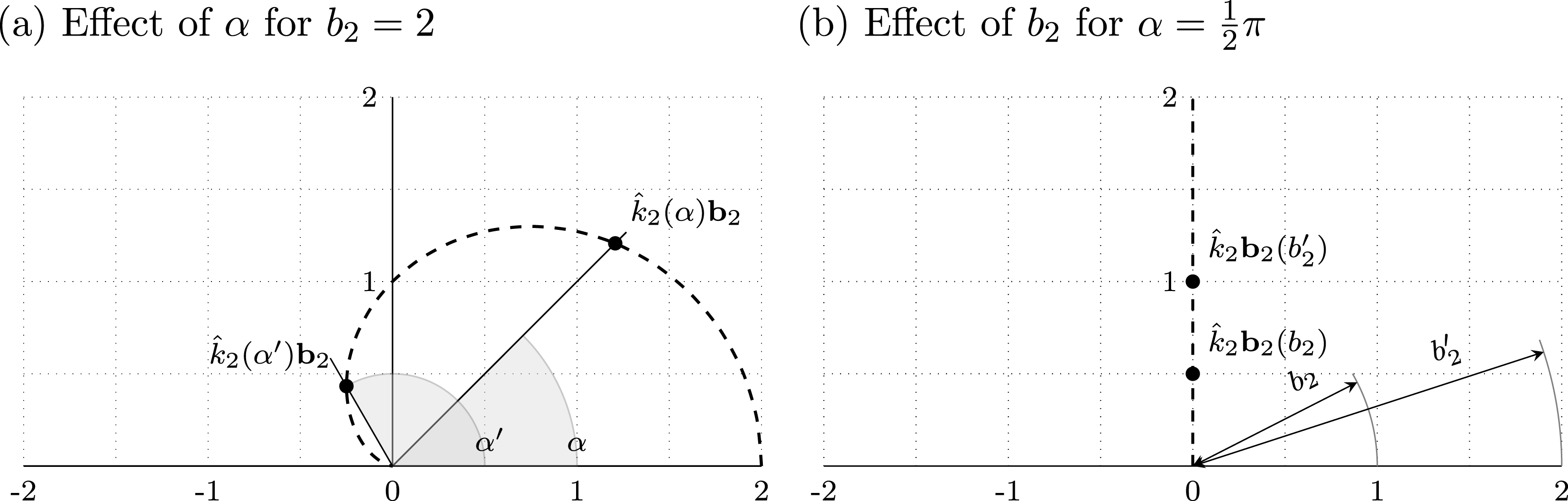
Figure 5 shows how the two parties’ equilibrium strategies change when we increase the value of
 $\unicode[STIX]{x1D6FC}$
(Figure 5a) and
 $b_{2}$
(Figure 5b), in the limit as
 $\unicode[STIX]{x1D6FF}\rightarrow 1$
. We focus here on the case where the initial incumbent’s policy commitment is sufficiently far from the origin to generate interesting policy dynamics. When the initial incumbent’s policy commitment is sufficiently close to the origin—that is, closer than
 $\hat{k}_{2}\mathbf{b}_{2}$
—neither
 $\unicode[STIX]{x1D6FC}$
nor
 $b_{2}$
matter for the moderation of implemented policies: in this case, neither party has an incentive to moderate further and the distance of implemented policies from the representative voter’s ideal policy stays constant.Footnote
14
We know from Proposition 1 and the discussion above that, when the initial incumbent’s policy commitment is sufficiently far from the origin, the equilibrium policies converge, in at most two periods, to alternation between
 $\hat{k}_{2}\mathbf{b}_{2}$
and
 $k_{1}(\hat{k}_{2}\mathbf{b}_{2})\mathbf{b}_{1}$
. Figure 5 shows the policy implemented whenever party
 $2$
is in power,
 $\hat{k}_{2}\mathbf{b}_{2}$
.Footnote
15
While this neglects a component of the representative voter’s ex ante welfare—which also depends on the policy implemented by party 1—it captures the main intuition.Footnote
16
The dashed line in both figures traces
 $\hat{k}_{2}\mathbf{b}_{2}$
as
 $\unicode[STIX]{x1D6FC}$
increases from 0 to
 $\unicode[STIX]{x1D70B}$
, and as
 $b_{2}$
increases from 0 to 4 (
 $b_{1}$
can be arbitrary on both figures provided
 $b_{1}>b_{2}$
).
When
 $\unicode[STIX]{x1D6FC}$
increases, the extent of ideological conflict between the two parties increases. This strengthens the strategic force to moderate and, thus, reduces
 $\hat{k}_{2}$
. Since the party’s bliss point is unchanged but the weight applied to it has decreased, the equilibrium policy of party 2,
 $\hat{k}_{2}\mathbf{b}_{2}$
, moves closer to the bliss point of the representative voter (Figure 5a). This clearly benefits the representative voter. Increasing the extremism of party 2,
 $b_{2}$
, on the other hand, has the opposite effect (Figure 5b). The strength of the moderating force does not change with
 $b_{2}$
and, thus,
 $\hat{k}_{2}$
is unchanged. Since the party’s bliss point has moved further away from the origin and the weight applied to it has not changed,
 $\hat{k}_{2}\mathbf{b}_{2}$
moves away from the origin too. Since the representative voter’s utility depends on the distance of the equilibrium policies from her bliss point, this has a negative effect on her welfare. Why does
 $\hat{k}_{2}$
depend on
 $\unicode[STIX]{x1D6FC}$
but not on
 $b_{2}$
(or
 $b_{1}$
)? Increasing extremism increases both the marginal benefit of moderation (that is, the gain from constraining the future incumbent to more moderate policies) and the marginal cost of moderation (that is, the loss from implementing policies further away from the bliss point), leaving their ratio constant. On the other hand, increasing antagonism has no influence on the marginal costs of moderation but it increases its marginal benefits.Footnote
17
 $^{\text{,}}$
Footnote
18
The next result presents the marginal impact of antagonism and extremism on the variance of the long-run policy outcomes. This is an interesting prediction as it allows us to link preferences’ disagreement to policy volatility. Denote with
 $d_{p}=d(\hat{k}_{2}\mathbf{b}_{2},k_{1}(\hat{k}_{2}\mathbf{b}_{2})\mathbf{b}_{1})$
the distance between the two long-run policies in the unique SSMPE from Proposition 1. This measure determines the variance of the long-run equilibrium policies characterized above.
Proposition 3. Assume that
 $b_{1}>b_{2}$
.
 $d_{p}$
is:
1. nondecreasing in
$b_{2}$
; increasing in
$b_{2}$
if
$\unicode[STIX]{x1D6FC}>0$
; constant in
$b_{1}$
;2. increasing in
$\unicode[STIX]{x1D6FC}$
when
$\unicode[STIX]{x1D6FC}\in [0,\unicode[STIX]{x1D6FC}^{\prime }]$
and decreasing in
$\unicode[STIX]{x1D6FC}$
when
$\unicode[STIX]{x1D6FC}\in [\unicode[STIX]{x1D6FC}^{\prime },\unicode[STIX]{x1D70B}]$
, where
$\unicode[STIX]{x1D6FC}^{\prime }\in [0,\unicode[STIX]{x1D70B}]$
and
$\unicode[STIX]{x1D6FC}^{\prime }<\unicode[STIX]{x1D70B}\Leftrightarrow \unicode[STIX]{x1D6FF}>\frac{1}{5}$
.


Proof. See Appendix A.☐
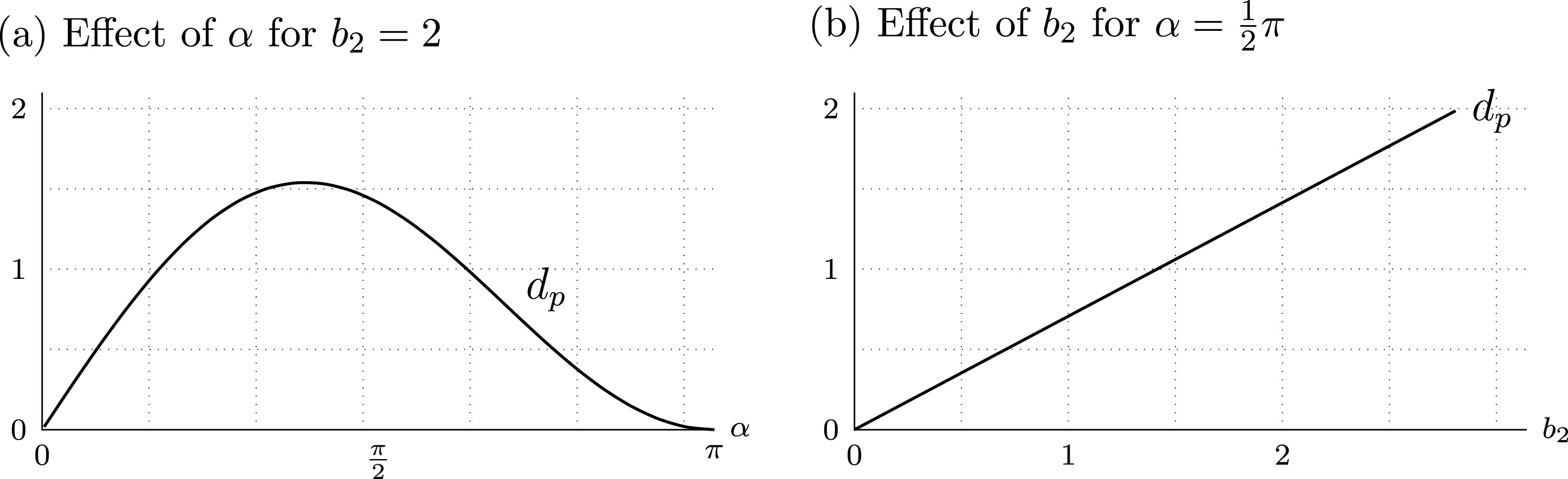
Figure 6 shows how the long-run policies variance change when we increase
 $\unicode[STIX]{x1D6FC}$
(Figure 6a) and
 $b_{2}$
(Figure 6b), in the limit as
 $\unicode[STIX]{x1D6FF}\rightarrow 1$
. Increasing the extremism of party
 $2$
has a straightforward effect on policy volatility, as it pushes the implemented policies away from the representative voter’s ideal point in different directions. Increasing the extremism of party 1, on other hand, has no effect because the long-run equilibrium policies depend only on the degree of moderation of party 2.Footnote
19
Finally, increasing antagonism has two effects: it distances the long-run policies away from each other but it also moves them closer to the ideal point of the representative voter. The former effects dominates for low
 $\unicode[STIX]{x1D6FC}$
, while the latter dominates for high
 $\unicode[STIX]{x1D6FC}$
.
 $d_{p}$
as a function of
 $\unicode[STIX]{x1D6FC}$
and
 $b_{2}$
 $\unicode[STIX]{x1D6FF}\rightarrow 1$
and
 $b_{1}>b_{2}$
.

7 Discussion and Conclusions
While many commentators and scholars diagnose a sharp and increasing ideological division between political elites in the United States and other mature democracies, both the popular press and the existing literature are somewhat unclear about what exactly constitutes polarization and how one can measure this concept.
In this paper, we study an environment where two ideological and forward-looking parties compete for office in a sequence of elections. We assume that incumbents who are reelected find it too costly to implement policies that differ from those of their first term. On the other hand, challengers are free to offer to the representative voter any policy platform. We use two different measures to describe the political environment and the degree of conflict among agents’ preferences. The first measure, which we label extremism, is the ideological distance of each party from the representative voter. The second measure, which we call antagonism, is the ideological distance that separates the two parties from each other and summarizes the degree of political competition between policymakers. These two measures coincide in a one-dimensional policy space, where the ideological distance between the two parties can increase only as they move further away from a moderate representative voter. However, they do not coincide in a two-dimensional setting: here, the two parties can be very close—when they share views on both dimensions—or very different—when they are perfectly opposed in one dimension—without altering their overall distance from the representative voter.
We show that a stationary Markov perfect equilibrium of this game exists and we fully characterize it for any discount factor, initial incumbent’s policy, and degree of extremism and antagonism. In this equilibrium, increasing the degree of extremism reduces the welfare of the representative voter; on the other hand, increasing antagonism increases the influence exerted by the electorate on long-run policy outcomes.Footnote 20
To conclude, we discuss the methodological and empirical implications of our model. Our analysis suggests that, in order to understand whether the electorate is better or worse off with increasingly polarized parties, social scientists need to be careful about how they measure polarization. Observing that parties’ ideal points are moving further away from each other does not necessarily imply that voters will suffer. In fact, this crucially depends on the distance between the parties’ and the voters’ ideal points. It is, thus, important to gauge both measures.
The existing empirical literature on ideological polarization has mostly measured the ideal points of parties and has ignored the electorate. Poole and Rosenthal (Reference Poole and Rosenthal1997) used roll call voting choices and item response models to estimate the relative ideological leanings of U.S. Congressmen, yielding what are called NOMINATE scores. Similar techniques were then used to estimate multidimensional ideal points of European parties, U.S. state legislators, and other elected officials. In recent years, Bayesian approaches have been applied to the problem of recovering preferences from observed choices, electoral platforms, or election results.Footnote 21
A key limitation of these estimations comes from the fact that ideal points are only defined relatively and two separate sets of ideal point estimates are, in general, not comparable. Our theoretical approach suggests that, to evaluate the policy and welfare consequences of polarization, we need ideal point estimates for both elected officials and voters, and, importantly, that we need these ideal points to be comparable or, in other words, to reside in a common policy space. The measures mentioned above, for example the NOMINATE scores, do not do this and, focusing on politicians’ ideal points, they are likely to capture what we label as antagonism, ignoring extremism.
As a consequence, the increasing distance between the main American parties on these measures—for example, the divergence in NOMINATE scores between the median Republican and the median Democrat in Congress—does not necessarily imply more extreme policies nor that the electorate is worse off. If parties are moving further away from each other and from the electorate, then increased elite polarization coincides with increased extremism, using the language of our model, and this is likely bad news for the moderate voters: as polarization increases, the observed policies will be more extreme, even when parties are forward-looking and policy motivated. On the other hand, if the increased ideological conflict between parties is associated with an unchanged distance from the median voter’s preferences—which can happen when the ideological conflict among actors is on multiple dimensions—this might be good news for moderate voters: the heightened competition between parties will not favor the civility of the political discourse and might lead to policy gridlock, but forward-looking and policy motivated parties will propose more moderate policies. It is not possible to distinguish between these two predictions without measuring jointly the ideological positions of the parties and the electorate.
In recent years, political scientists have started to bridge this gap and have attempted to measure the ideological position of elected leaders and members of the public on a common policy space (see, for example, Jessee Reference Jessee2009, Reference Jessee2010; Bafumi and Herron Reference Bafumi and Herron2010; Bonica Reference Bonica2014; Lo, Proksch, and Gschwend Reference Lo, Proksch and Gschwend2014; Barbera Reference Barbera2015). While these are important advances, the existing works suffer from some important shortcomings that hinder our ability to evaluate the normative consequences of polarization through the lenses of our theoretical results: most of these studies rely on survey questions to gauge the ideal points of voters and assume these responses are directly comparable with roll call votes on the same issues; more importantly, they assume that policies and preferences are unidimensional—making it impossible to disentangle antagonism and extremism—and focus on a short time span (a single election or, at most, two U.S. Congresses).
Our theoretical analysis supports this recent direction and highlights the importance for future empirical research in legislative studies and political behavior of exploring multiple policy dimensions and time trends. Over time, the research program being advanced by these scholars, together with the predictions of dynamic models of elections, can be used to provide a nuanced perspective on the impact of elite polarization on implemented policies and electorate’s welfare.
Appendix A. Proofs
Proof of Proposition 1
Let
 $\hat{k}_{1}$
and
 $\hat{k}_{2}$
be the parameters associated with simple strategies and let
 $\hat{k}_{1}^{\ast }$
and
 $\hat{k}_{2}^{\ast }$
be the parameters associated with the simple strategies of a SSMPE (as described in Definition 3). When talking about both parameters jointly, we use
 $\hat{k}=(\hat{k}_{1},\hat{k}_{2})$
and
 $\hat{k}^{\ast }=(\hat{k}_{1}^{\ast },\hat{k}_{2}^{\ast })$
. Because a simple strategy of
 $i\in \{1,2\}$
from Definition 3 is fully determined by
 $\hat{k}_{i}$
, with a slight abuse of notation, we call
 $\hat{k}_{i}$
the strategy of
 $i$
and
 $\hat{k}=(\hat{k}_{1},\hat{k}_{2})$
the profile of strategies.
We start by noting that any SSMPE strategy of
 $v$
satisfies, for an incumbent
 $j\in \{1,2\}$
, its policy commitment
 $\mathbf{q}\in X$
and a platform of the opposition
 $\mathbf{p}\in X$
,
 $\unicode[STIX]{x1D70E}_{v}^{\ast }(\,j,\mathbf{q},\mathbf{p})=\mathit{Yes}$
if and only if
 $d(\mathbf{p})\leqslant d(\mathbf{q})$
. From Definition 2,
 $\unicode[STIX]{x1D70E}_{v}^{\ast }(\,j,\mathbf{q},\mathbf{p})=\mathit{Yes}$
if and only if
 $u_{v}(\mathbf{p})\geqslant u_{v}(\mathbf{q})$
, which, from
 $u_{v}(\mathbf{x})=-d^{2}(\mathbf{x})$
for any
 $\mathbf{x}\in X$
, is equivalent to
 $d(\mathbf{p})\leqslant d(\mathbf{q})$
. Because of the simplicity of the representative voter’s behavior in any SSMPE, we suppress
 $\unicode[STIX]{x1D70E}_{v}$
from the notation below.
We now claim that, for any SSMPE strategy of
 $v$
and any simple strategy profile of the two parties
 $\hat{k}$
, the opposition party contests elections and wins. The former follows from
 $\mathbf{p}_{i}(\mathbf{q})\neq Out$
for any
 $i\in \{1,2\}$
,
 $\hat{k}_{i}\in \mathbb{R}$
and
 $\mathbf{q}\in X$
. To prove the latter claim, we need to show that
 $d(\mathbf{p}_{i}(\mathbf{q}))\leqslant d(\mathbf{q})$
for any
 $i\in \{1,2\}$
,
 $\hat{k}_{i}\in \mathbb{R}$
and
 $\mathbf{q}\in X$
. From Definition 3, if
 $k_{i}(\mathbf{q})\leqslant \hat{k}_{i}$
, then
 $d(\mathbf{p}_{i}(\mathbf{q}))=d(k_{i}(\mathbf{q})\mathbf{b}_{i})=k_{i}(\mathbf{q})b_{i}=\frac{d(\mathbf{q})}{b_{i}}b_{i}$
and if
 $k_{i}(\mathbf{q})\geqslant \hat{k}_{i}$
, then
 $d(\mathbf{p}_{i}(\mathbf{q}))=d(\hat{k}_{i}\mathbf{b}_{i})=\hat{k}_{i}b_{i}\leqslant k_{i}(\mathbf{q})b_{i}=d(\mathbf{q})$
. Because the opposition party contests elections and wins for any SSMPE strategy of
 $v$
and any simple strategy profile
 $\hat{k}$
, elections are always contested and incumbents always defeated in any SSMPE. This proves part 3 of the proposition.
We now prove parts 1 (characterization) and 2 (uniqueness or duplicity) of the proposition. By the one-stage-deviation principle, a profile of strategies
 $\hat{k}^{\ast }$
constitutes a SSMPE if, for any
 $i\in \{1,2\}$
and
 $\mathbf{q}\in X$
, a deviation by the opposition party
 $i$
to contest elections with
 $\mathbf{p}\neq \mathbf{p}_{i}(\mathbf{q})$
or to stay out is not profitable. We momentarily assume and later verify that both parties, when at the opposition, want to contest elections with platforms that guarantee their victory.
For any
 $\hat{k}$
,
 $i\in \{1,2\}$
and
 $\mathbf{q}\in X$
, the dynamic utility
 $i$
receives from running with
 $\mathbf{p}$
such that
 $d(\mathbf{p})\leqslant d(\mathbf{q})$
is
 $u_{i}(\mathbf{p})+r+\unicode[STIX]{x1D6FF}V_{i}^{i}(\mathbf{p}|\hat{k})$
. An opposition party
 $i$
thus runs with
 $\mathbf{p}^{\ast }\in \operatorname{argmax}_{d(\mathbf{x})\leqslant d(\mathbf{q})}u_{i}(\mathbf{x})+r+\unicode[STIX]{x1D6FF}V_{i}^{i}(\mathbf{x}|\hat{k})$
. For any
 $\hat{k}$
and any two policies
 $\mathbf{p}\in X$
and
 $\mathbf{p}^{\prime }\in X$
with
 $d(\mathbf{p})=d(\mathbf{p}^{\prime })$
, we have
 $V_{i}^{i}(\mathbf{p}|\hat{k})=V_{i}^{i}(\mathbf{p}^{\prime }|\hat{k})$
. This means that the optimal
 $\mathbf{p}^{\ast }$
has to lie on the ray starting at
 $\mathbf{b}_{v}=(0,0)$
and passing through
 $\mathbf{b}_{i}$
. It hence can be written as
 $\mathbf{p}^{\ast }=k\mathbf{b}_{i}$
for some
 $k\geqslant 0$
. Denote by
 $U_{i}(k|\hat{k})=u_{i}(k\mathbf{b}_{i})+r+\unicode[STIX]{x1D6FF}V_{i}^{i}(k\mathbf{b}_{i}|\hat{k})$
the dynamic utility of party
 $i\in \{1,2\}$
from running with policy
 $k\mathbf{b}_{i}$
when the parties use simple strategies characterized by
 $\hat{k}$
. The key properties of
 $U_{i}(k|\hat{k})$
are summarized in the lemma below. To facilitate its proof, we first state several identities for the policy utility of the two parties.
The policy utility
 $i\in \{1,2\}$
derives from
 $k\mathbf{b}_{j}$
where
 $k\geqslant 0$
and
 $j\in \{1,2\}$
is
 $u_{i}(k\mathbf{b}_{j})=-d^{2}(k\mathbf{b}_{j},\mathbf{b}_{i})$
. This is a continuous and differentiable function of
 $k$
. Using
 $-i=\{1,2\}\setminus \{i\}$
, we have
 $$\begin{eqnarray}\begin{array}{@{}ll@{}}{\displaystyle \frac{\unicode[STIX]{x2202}(-d^{2}(k\mathbf{b}_{-i},\mathbf{b}_{i}))}{\unicode[STIX]{x2202}k}} & \displaystyle =-2(kd^{2}(\mathbf{b}_{-i})-\mathbf{b}_{-i}\cdot \mathbf{b}_{i})=-2b_{i}b_{-i}\left(k{\textstyle \frac{b_{-i}}{b_{i}}}-\cos \unicode[STIX]{x1D6FC}\right)\\ {\displaystyle \frac{\unicode[STIX]{x2202}(-d^{2}(k\mathbf{b}_{i},\mathbf{b}_{i}))}{\unicode[STIX]{x2202}k}} & \displaystyle =-2(kd^{2}(\mathbf{b}_{i})-\mathbf{b}_{i}\cdot \mathbf{b}_{i})=-2b_{i}^{2}(k-1)\\ {\displaystyle \frac{\unicode[STIX]{x2202}^{2}(-d^{2}(k\mathbf{b}_{j},\mathbf{b}_{i}))}{\unicode[STIX]{x2202}^{2}k}} & \displaystyle =-2d^{2}(\mathbf{b}_{j}).\end{array}\end{eqnarray}$$
This proves that
 $u_{i}(k\mathbf{b}_{j})$
is a concave function of
 $k$
.
Lemma A1. For any
 $i\in \{1,2\}$
, fix
 $\hat{k}_{i}\in \mathbb{R}$
and
 $\hat{k}_{-i}\in \mathbb{R}$
. Let
 $\mathbf{q}\in X$
be the incumbent’s policy commitment.
 $U_{i}(k|\hat{k})$
, as a function of
 $k\in [0,k_{i}(\mathbf{q})]$
, is continuous, differentiable except when
 $k=\hat{k}_{i}$
or
 $k=\hat{k}_{-i}\frac{b_{-i}}{b_{i}}$
, strictly concave on each interval on which it is differentiable and
 $\frac{\unicode[STIX]{x2202}U_{i}(k|\hat{k})}{\unicode[STIX]{x2202}k}>0$
for
 $k<c$
,
 $\frac{\unicode[STIX]{x2202}U_{i}(k|\hat{k})}{\unicode[STIX]{x2202}k}=0$
for
 $k=c$
and
 $\frac{\unicode[STIX]{x2202}U_{i}(k|\hat{k})}{\unicode[STIX]{x2202}k}<0$
for
 $k>c$
where
 $$\begin{eqnarray}\begin{array}{@{}llll@{}}c= & \,{\textstyle \frac{1+\unicode[STIX]{x1D6FF}\cos \unicode[STIX]{x1D6FC}}{1+\unicode[STIX]{x1D6FF}}} & & \text{ if }k<\min \{\hat{k}_{i},\hat{k}_{-i}{\textstyle \frac{b_{-i}}{b_{i}}}\}\\ c= & \,{\textstyle \frac{1+\unicode[STIX]{x1D6FF}\cos \unicode[STIX]{x1D6FC}}{1+\unicode[STIX]{x1D6FF}}} & & \text{ if }\hat{k}_{i}<k<\hat{k}_{-i}{\textstyle \frac{b_{-i}}{b_{i}}}\\ c= & \,1 & & \text{ if }\hat{k}_{-i}{\textstyle \frac{b_{-i}}{b_{i}}}<k<\hat{k}_{i}\\ c= & \,1 & & \text{ if }\max \{\hat{k}_{i},\hat{k}_{-i}{\textstyle \frac{b_{-i}}{b_{i}}}\}<k.\\ \end{array}\end{eqnarray}$$
Proof. Throughout the proof fix
 $i\in \{1,2\}$
,
 $-i=\{1,2\}\setminus \{i\}$
,
 $\hat{k}_{i}\in \mathbb{R}$
,
 $\hat{k}_{-i}\in \mathbb{R}$
and incumbent’s policy commitment
 $\mathbf{q}\in X$
. The continuity is easy to see as the simple strategies characterized by
 $\hat{k}$
give rise to a value function,
 $V_{i}^{i}(\mathbf{x}|\hat{k})$
, that is continuous in
 $\mathbf{x}\in X$
for any
 $d(\mathbf{x})\leqslant d(\mathbf{q})$
. For the remaining properties, we have to derive
 $V_{i}^{i}(\mathbf{x}|\hat{k})$
explicitly. Because the opposition party always contests and wins elections for any
 $\hat{k}$
, we have, for any
 $\mathbf{x}\in X$
with
 $d(\mathbf{x})\leqslant d(\mathbf{q})$
,
 $$\begin{eqnarray}\begin{array}{@{}rl@{}}V_{i}^{-i}(\mathbf{x}|\hat{k}) & \displaystyle =u_{i}(\mathbf{p}_{i}(\mathbf{x}))+r+\unicode[STIX]{x1D6FF}V_{i}^{i}(\mathbf{p}_{i}(\mathbf{x})|\hat{k})\\ V_{i}^{i}(\mathbf{x}|\hat{k}) & \displaystyle =u_{i}(\mathbf{p}_{-i}(\mathbf{x}))+\unicode[STIX]{x1D6FF}V_{i}^{-i}(\mathbf{p}_{-i}(\mathbf{x})|\hat{k}).\\ \end{array}\end{eqnarray}$$
Combining the two equations
 $$\begin{eqnarray}V_{i}^{i}(\mathbf{x}|\hat{k})=u_{i}(\mathbf{p}_{-i}(\mathbf{x}))+\unicode[STIX]{x1D6FF}\left[u_{i}(\mathbf{p}_{i}(\mathbf{p}_{-i}(\mathbf{x})))+r+\unicode[STIX]{x1D6FF}V_{i}^{i}(\mathbf{p}_{i}(\mathbf{p}_{-i}(\mathbf{x}))|\hat{k})\right]\end{eqnarray}$$
where
 $$\begin{eqnarray}\begin{array}{@{}llllll@{}}\mathbf{p}_{-i}(\mathbf{x}) & \displaystyle =k_{i}(\mathbf{x}){\textstyle \frac{b_{i}}{b_{-i}}}\mathbf{b}_{-i} & \quad \mathbf{p}_{i}(\mathbf{p}_{-i}(\mathbf{x})) & \displaystyle =k_{i}(\mathbf{x})\mathbf{b}_{i} & & \text{if }k_{i}(x)\leqslant \min \{\hat{k}_{i},\hat{k}_{-i}{\textstyle \frac{b_{-i}}{b_{i}}}\}\\ \mathbf{p}_{-i}(\mathbf{x}) & \displaystyle =k_{i}(\mathbf{x}){\textstyle \frac{b_{i}}{b_{-i}}}\mathbf{b}_{-i} & \quad \mathbf{p}_{i}(\mathbf{p}_{-i}(\mathbf{x})) & \displaystyle =\hat{k}_{i}\mathbf{b}_{i} & & \text{if }\hat{k}_{i}<k_{i}(x)<\hat{k}_{-i}{\textstyle \frac{b_{-i}}{b_{i}}}\\ \mathbf{p}_{-i}(\mathbf{x}) & \displaystyle =\hat{k}_{-i}\mathbf{b}_{-i} & \quad \mathbf{p}_{i}(\mathbf{p}_{-i}(\mathbf{x})) & \displaystyle =\hat{k}_{-i}{\textstyle \frac{b_{-i}}{b_{i}}}\mathbf{b}_{i} & & \text{if }\hat{k}_{-i}{\textstyle \frac{b_{-i}}{b_{i}}}<k_{i}(x)<\hat{k}_{i}\\ \mathbf{p}_{-i}(\mathbf{x}) & \displaystyle =\hat{k}_{-i}\mathbf{b}_{-i} & \quad \mathbf{p}_{i}(\mathbf{p}_{-i}(\mathbf{x})) & \displaystyle =\min \{\hat{k}_{-i}{\textstyle \frac{b_{-i}}{b_{i}}},\hat{k}_{i}\}\mathbf{b}_{i} & & \text{if }\max \{\hat{k}_{i},\hat{k}_{-i}{\textstyle \frac{b_{-i}}{b_{i}}}\}\leqslant k_{i}(x)\end{array}\end{eqnarray}$$
is easy to confirm using properties of the simple strategies along with
 $k_{i}(\mathbf{x})b_{i}=k_{-i}(\mathbf{x})b_{-i}$
for any
 $\mathbf{x}\in X$
.
We substitute
 $\mathbf{x}=k\mathbf{b}_{i}$
into (A 4), using (A 5),
 $k_{i}(k\mathbf{b}_{i})=k$
,
 $u_{i}(\mathbf{x})=-d^{2}(\mathbf{x},\mathbf{b}_{i})$
and
 $V_{i}^{i}(\mathbf{x}|\hat{k})=V_{i}^{i}(k_{i}(\mathbf{x})\mathbf{b}_{i}|\hat{k})$
, which follows from
 $d(k_{i}(\mathbf{x})\mathbf{b}_{i})=\frac{d(\mathbf{x})}{b_{i}}d(\mathbf{b}_{i})=d(\mathbf{x})$
. After some straightforward algebra, summarizing with
 $\unicode[STIX]{x1D712}_{t}$
all the terms constant in
 $k$
, we have:
 $$\begin{eqnarray}\begin{array}{@{}llll@{}}U_{i}(k|\hat{k}) & \displaystyle ={\displaystyle \frac{-d^{2}(k\mathbf{b}_{i},\mathbf{b}_{i})-d^{2}(k{\textstyle \frac{b_{i}}{b_{-i}}}\mathbf{b}_{-i},\mathbf{b}_{i})\unicode[STIX]{x1D6FF}+r}{1-\unicode[STIX]{x1D6FF}^{2}}} & & \text{if }k\leqslant \min \{\hat{k}_{i},\hat{k}_{-i}{\textstyle \frac{b_{-i}}{b_{i}}}\}\\ U_{i}(k|\hat{k}) & \displaystyle =-d^{2}(k\mathbf{b}_{i},\mathbf{b}_{i})-d^{2}(k{\textstyle \frac{b_{i}}{b_{-i}}}\mathbf{b}_{-i},\mathbf{b}_{i})\unicode[STIX]{x1D6FF}+\unicode[STIX]{x1D712}_{1} & & \text{if }\hat{k}_{i}<k<\hat{k}_{-i}{\textstyle \frac{b_{-i}}{b_{i}}}\\ U_{i}(k|\hat{k}) & \displaystyle =-d^{2}(k\mathbf{b}_{i},\mathbf{b}_{i})+\unicode[STIX]{x1D712}_{2} & & \text{if }\hat{k}_{-i}{\textstyle \frac{b_{-i}}{b_{i}}}<k<\hat{k}_{i}\\ U_{i}(k|\hat{k}) & \displaystyle =-d^{2}(k\mathbf{b}_{i},\mathbf{b}_{i})+\unicode[STIX]{x1D712}_{3} & & \text{if }\max \{\hat{k}_{i},\hat{k}_{-i}{\textstyle \frac{b_{-i}}{b_{i}}}\}\leqslant k\\ \end{array}\end{eqnarray}$$
for any
 $k\in [0,k_{i}(\mathbf{q})]$
. Direct verification then shows all the remaining properties of
 $U_{i}(k|\hat{k})$
.Footnote
22
☐
Using
 $U_{i}(k|\hat{k})$
we can rewrite the optimization problem of opposition party
 $i\in \{1,2\}$
regarding which policy to contest elections with, for any incumbent’s policy commitment
 $\mathbf{q}\in X$
, as
 $\max _{0\leqslant k\leqslant k_{i}(\mathbf{q})}U_{i}(k|\hat{k})$
. To find a SSMPE, we need to find a
 $\hat{k}^{\ast }$
such that the solution to this optimization problem under
 $\hat{k}^{\ast }$
, for any
 $\mathbf{q}\in X$
, can be described by
 $\hat{k}^{\ast }$
.
We first claim that in any SSMPE,
 $\hat{k}_{i}^{\ast }\in \{\!\frac{1+\unicode[STIX]{x1D6FF}\cos \unicode[STIX]{x1D6FC}}{1+\unicode[STIX]{x1D6FF}},1\!\}$
for
 $i\in \{1,2\}$
. Notice
 $\frac{1+\unicode[STIX]{x1D6FF}\cos \unicode[STIX]{x1D6FC}}{1+\unicode[STIX]{x1D6FF}}\leqslant 1$
for any
 $\unicode[STIX]{x1D6FF}\in [0,1)$
and
 $\unicode[STIX]{x1D6FC}\in [0,\unicode[STIX]{x1D70B}]$
. To show the claim, suppose, toward a first contradiction, that
 $\hat{k}_{i}^{\ast }<\frac{1+\unicode[STIX]{x1D6FF}\cos \unicode[STIX]{x1D6FC}}{1+\unicode[STIX]{x1D6FF}}$
. Suppose
 $\hat{k}_{-i}^{\ast }\frac{b_{-i}}{b_{i}}\leqslant \hat{k}_{i}^{\ast }$
. Then from Lemma A1, there exists
 $\bar{\unicode[STIX]{x1D716}}>0$
such that for all
 $\unicode[STIX]{x1D716}\in (0,\bar{\unicode[STIX]{x1D716}})$
,
 $U_{i}^{\prime }(\hat{k}_{i}^{\ast }+\unicode[STIX]{x1D716}|\hat{k}^{\ast })>0$
, which implies that
 $U_{i}(\hat{k}_{i}^{\ast }|\hat{k}^{\ast })<U_{i}(\hat{k}_{i}^{\ast }+\unicode[STIX]{x1D716}|\hat{k}^{\ast })$
,
 $\mathbf{p}_{i}((\hat{k}_{i}^{\ast }+\unicode[STIX]{x1D716})\mathbf{b}_{i})=\hat{k}_{i}^{\ast }\mathbf{b}_{i}$
and
 $d((\hat{k}_{i}^{\ast }+\unicode[STIX]{x1D716})\mathbf{b}_{i})<d((\hat{k}_{i}^{\ast }+\bar{\unicode[STIX]{x1D716}})\mathbf{b}_{i})$
. In words, for incumbent’s policy commitment
 $(\hat{k}_{i}^{\ast }+\bar{\unicode[STIX]{x1D716}})\mathbf{b}_{i}$
,
 $i$
contests elections with
 $\hat{k}_{i}^{\ast }\mathbf{b}_{i}$
, despite the fact that running with
 $(\hat{k}_{i}^{\ast }+\unicode[STIX]{x1D716})\mathbf{b}_{i}$
would ensure its victory and higher dynamic utility, a contradiction. An identical argument leads to a contradiction when
 $\hat{k}_{-i}^{\ast }\frac{b_{-i}}{b_{i}}>\hat{k}_{i}^{\ast }$
. Now suppose, toward a second contradiction, that
 $\hat{k}_{i}^{\ast }\in (\frac{1+\unicode[STIX]{x1D6FF}\cos \unicode[STIX]{x1D6FC}}{1+\unicode[STIX]{x1D6FF}},1)$
. If
 $\hat{k}_{-i}^{\ast }\frac{b_{-i}}{b_{i}}\leqslant \hat{k}_{i}^{\ast }$
, an argument identical to the one above leads to a contradiction. Suppose
 $\hat{k}_{-i}^{\ast }\frac{b_{-i}}{b_{i}}>\hat{k}_{i}^{\ast }$
. Then from Lemma A1, there exists
 $\bar{\unicode[STIX]{x1D716}}>0$
such that for all
 $\unicode[STIX]{x1D716}\in (0,\bar{\unicode[STIX]{x1D716}})$
,
 $U_{i}^{\prime }(\frac{1+\unicode[STIX]{x1D6FF}\cos \unicode[STIX]{x1D6FC}}{1+\unicode[STIX]{x1D6FF}}+\unicode[STIX]{x1D716}|\hat{k}^{\ast })<0$
, which implies that
 $U_{i}(\frac{1+\unicode[STIX]{x1D6FF}\cos \unicode[STIX]{x1D6FC}}{1+\unicode[STIX]{x1D6FF}}|\hat{k}^{\ast })>U_{i}(\frac{1+\unicode[STIX]{x1D6FF}\cos \unicode[STIX]{x1D6FC}}{1+\unicode[STIX]{x1D6FF}}+\unicode[STIX]{x1D716}|\hat{k}^{\ast })$
,
 $\mathbf{p}_{i}((\frac{1+\unicode[STIX]{x1D6FF}\cos \unicode[STIX]{x1D6FC}}{1+\unicode[STIX]{x1D6FF}}+\unicode[STIX]{x1D716})\mathbf{b}_{i})=(\frac{1+\unicode[STIX]{x1D6FF}\cos \unicode[STIX]{x1D6FC}}{1+\unicode[STIX]{x1D6FF}}+\unicode[STIX]{x1D716})\mathbf{b}_{i}$
and
 $d(\frac{1+\unicode[STIX]{x1D6FF}\cos \unicode[STIX]{x1D6FC}}{1+\unicode[STIX]{x1D6FF}}\mathbf{b}_{i})<d((\frac{1+\unicode[STIX]{x1D6FF}\cos \unicode[STIX]{x1D6FC}}{1+\unicode[STIX]{x1D6FF}}+\bar{\unicode[STIX]{x1D716}})\mathbf{b}_{i})$
, a contradiction. Finally suppose, toward a third contradiction, that
 $\hat{k}_{i}^{\ast }>1$
. Then irrespective of
 $\hat{k}_{-i}^{\ast }$
, Lemma A1 implies that there exists
 $\bar{\unicode[STIX]{x1D716}}>0$
such that, for all
 $\unicode[STIX]{x1D716}\in (0,\bar{\unicode[STIX]{x1D716}})$
,
 $U_{i}^{\prime }(1+\unicode[STIX]{x1D716}|\hat{k}^{\ast })<0$
, which implies that
 $U_{i}(1|\hat{k}^{\ast })>U_{i}(1+\unicode[STIX]{x1D716}|\hat{k}^{\ast })$
,
 $\mathbf{p}_{i}((1+\unicode[STIX]{x1D716})\mathbf{b}_{i})=(1+\unicode[STIX]{x1D716})\mathbf{b}_{i}$
and
 $d(\mathbf{b}_{i})<d((1+\bar{\unicode[STIX]{x1D716}})\mathbf{b}_{i})$
, a contradiction.
Having shown that
 $\hat{k}_{i}^{\ast }\in \{\!\frac{1+\unicode[STIX]{x1D6FF}\cos \unicode[STIX]{x1D6FC}}{1+\unicode[STIX]{x1D6FF}},1\!\}$
for
 $i\in \{1,2\}$
, we now argue that
 $\hat{k}_{i}^{\ast }=\frac{1+\unicode[STIX]{x1D6FF}\cos \unicode[STIX]{x1D6FC}}{1+\unicode[STIX]{x1D6FF}}$
for all
 $i\in \{1,2\}$
cannot constitute an SSMPE unless
 $\frac{1+\unicode[STIX]{x1D6FF}\cos \unicode[STIX]{x1D6FC}}{1+\unicode[STIX]{x1D6FF}}=1$
, that is unless
 $\unicode[STIX]{x1D6FF}=0$
or
 $\unicode[STIX]{x1D6FC}=0$
. Suppose, toward a contradiction, that
 $\unicode[STIX]{x1D6FF}>0$
,
 $\unicode[STIX]{x1D6FC}>0$
and
 $\hat{k}_{i}^{\ast }=\frac{1+\unicode[STIX]{x1D6FF}\cos \unicode[STIX]{x1D6FC}}{1+\unicode[STIX]{x1D6FF}}$
. This implies that
 $\hat{k}_{i}^{\ast }<1$
for all
 $i\in \{1,2\}$
. Suppose, without loss of generality, that
 $b_{1}\geqslant b_{2}$
. Then Lemma A1 implies that there exists
 $\bar{\unicode[STIX]{x1D716}}>0$
such that for all
 $\unicode[STIX]{x1D716}\in (0,\bar{\unicode[STIX]{x1D716}})$
,
 $U_{1}^{\prime }(\hat{k}_{1}^{\ast }+\unicode[STIX]{x1D716}|\hat{k}^{\ast })>0$
, which implies that
 $U_{1}(\hat{k}_{1}^{\ast }|\hat{k}^{\ast })<U_{1}(\hat{k}_{1}^{\ast }+\unicode[STIX]{x1D716}|\hat{k}^{\ast })$
,
 $\mathbf{p}_{1}((\hat{k}_{1}^{\ast }+\unicode[STIX]{x1D716})\mathbf{b}_{1})=\hat{k}_{1}^{\ast }\mathbf{b}_{1}$
and
 $d((\hat{k}_{1}^{\ast }+\unicode[STIX]{x1D716})\mathbf{b}_{1})<d((\hat{k}_{1}^{\ast }+\bar{\unicode[STIX]{x1D716}})\mathbf{b}_{1})$
, which means party
 $1$
is not maximizing its dynamic utility when at the opposition. Furthermore, an argument similar to the one used in the second contradiction above implies that
 $\hat{k}_{1}^{\ast }=\hat{k}_{2}^{\ast }=1$
cannot constitute an SSMPE unless
 $\unicode[STIX]{x1D6FF}=0$
or
 $\unicode[STIX]{x1D6FC}=0$
.
This leaves three possible cases. Case 1:
 $\unicode[STIX]{x1D6FF}=0$
or
 $\unicode[STIX]{x1D6FC}=0$
and
 $\hat{k}_{1}^{\ast }=\hat{k}_{2}^{\ast }=1$
. When
 $\unicode[STIX]{x1D6FF}=0$
or
 $\unicode[STIX]{x1D6FC}=0$
, clearly
 $\hat{k}^{\ast }=(1,1)$
constitutes a SSMPE and, because
 $\hat{k}_{i}^{\ast }\in \{\frac{1+\unicode[STIX]{x1D6FF}\cos \unicode[STIX]{x1D6FC}}{1+\unicode[STIX]{x1D6FF}},1\}$
for
 $i\in \{1,2\}$
, this SSMPE is unique. Case 2:
 $\unicode[STIX]{x1D6FF}>0$
and
 $\unicode[STIX]{x1D6FC}>0$
and
 $\hat{k}_{1}^{\ast }=1$
with
 $\hat{k}_{2}^{\ast }=\frac{1+\unicode[STIX]{x1D6FF}\cos \unicode[STIX]{x1D6FC}}{1+\unicode[STIX]{x1D6FF}}$
. Case 3:
 $\unicode[STIX]{x1D6FF}>0$
and
 $\unicode[STIX]{x1D6FC}>0$
and
 $\hat{k}_{1}^{\ast }=\frac{1+\unicode[STIX]{x1D6FF}\cos \unicode[STIX]{x1D6FC}}{1+\unicode[STIX]{x1D6FF}}$
with
 $\hat{k}_{2}^{\ast }=1$
.
We first claim that when
 $b_{1}>b_{2}$
, Case 3 cannot constitute a SSMPE. When
 $\unicode[STIX]{x1D6FF}>0$
and
 $\unicode[STIX]{x1D6FC}>0$
,
 $\frac{1+\unicode[STIX]{x1D6FF}\cos \unicode[STIX]{x1D6FC}}{1+\unicode[STIX]{x1D6FF}}<1$
. From
 $\hat{k}_{1}^{\ast }=\frac{1+\unicode[STIX]{x1D6FF}\cos \unicode[STIX]{x1D6FC}}{1+\unicode[STIX]{x1D6FF}}$
,
 $\hat{k}_{2}^{\ast }=1$
and
 $b_{1}>b_{2}$
, it follows
 $\frac{1+\unicode[STIX]{x1D6FF}\cos \unicode[STIX]{x1D6FC}}{1+\unicode[STIX]{x1D6FF}}b_{2}<b_{2}=\hat{k}_{2}^{\ast }b_{2}$
and
 $\frac{1+\unicode[STIX]{x1D6FF}\cos \unicode[STIX]{x1D6FC}}{1+\unicode[STIX]{x1D6FF}}b_{2}<\frac{1+\unicode[STIX]{x1D6FF}\cos \unicode[STIX]{x1D6FC}}{1+\unicode[STIX]{x1D6FF}}b_{1}=\hat{k}_{1}^{\ast }b_{1}$
, or
 $\frac{1+\unicode[STIX]{x1D6FF}\cos \unicode[STIX]{x1D6FC}}{1+\unicode[STIX]{x1D6FF}}<\min \{\hat{k}_{1}^{\ast }\frac{b_{1}}{b_{2}},\hat{k}_{2}^{\ast }\}$
. We can now use argument similar to the one used in the second contradiction above to establish contradiction with party
 $2$
maximizing its dynamic utility when in opposition.
It remains to be shown that, when
 $b_{1}>b_{2}$
, Case 2 constitutes a unique SSMPE and that, when
 $b_{1}=b_{2}$
, both Cases 2 and 3 constitute an SSMPE. We cover Case 2 irrespective of whether
 $b_{1}>b_{2}$
or
 $b_{1}=b_{2}$
. When
 $b_{1}=b_{2}$
, Case 3 is similar to Case 2 and is omitted.
Suppose
 $\unicode[STIX]{x1D6FF}>0$
,
 $\unicode[STIX]{x1D6FC}>0$
and
 $b_{1}\geqslant b_{2}$
. We need to show that
 $\hat{k}_{1}=1$
and
 $\hat{k}_{2}=\frac{1+\unicode[STIX]{x1D6FF}\cos \unicode[STIX]{x1D6FC}}{1+\unicode[STIX]{x1D6FF}}$
constitute an SSMPE. Take any incumbent’s policy commitment
 $\mathbf{q}\in X$
. The optimization problem of the opposition party regarding the policy to contest elections with is
 $\max _{k\in [0,k_{i}(\mathbf{q})]}U_{i}(k|\hat{k})$
. For any
 $\mathbf{q}\in X$
such that
 $k_{2}(\mathbf{q})>\hat{k}_{2}$
, from Lemma A1 we have
 $\lim _{k\rightarrow \hat{k}_{2}^{-}}U_{2}^{\prime }(k|\hat{k})\geqslant 0$
and
 $\lim _{k\rightarrow \hat{k}_{2}^{+}}U_{2}^{\prime }(k|\hat{k})\leqslant 0$
. By piece-wise strict concavity of
 $U_{2}$
established in the same lemma,
 $U_{2}(k|\hat{k})$
is, for any
 $\mathbf{q}\in X$
, increasing in
 $k$
on
 $[0,\min \{\hat{k}_{2},k_{2}(\mathbf{q})\}]$
and decreasing in
 $k$
on
 $[\hat{k}_{2},\max \{\hat{k}_{2},k_{2}(\mathbf{q})\}]$
. When
 $k_{2}(\mathbf{q})\leqslant \hat{k}_{2}$
, it is optimal for party
 $2$
to contest elections with
 $k_{2}(\mathbf{q})\mathbf{b}_{2}$
and when
 $k_{2}(\mathbf{q})>\hat{k}_{2}$
, it is optimal to run with
 $\hat{k}_{2}\mathbf{b}_{2}$
. The simple strategy with
 $\hat{k}_{2}$
is thus optimal for party 2. A similar argument can be used to show optimality of the simple strategy with
 $\hat{k}_{1}$
for party 1. The key to this claim is Lemma A1 along with
 $\hat{k}_{2}b_{2}<\hat{k}_{1}b_{1}$
and
 $\hat{k}_{2}b_{2}=\frac{1+\unicode[STIX]{x1D6FF}\cos \unicode[STIX]{x1D6FC}}{1+\unicode[STIX]{x1D6FF}}b_{2}<\frac{1+\unicode[STIX]{x1D6FF}\cos \unicode[STIX]{x1D6FC}}{1+\unicode[STIX]{x1D6FF}}b_{1}$
.
To finish the proof of parts 1 and 2 of the proposition, we have to show that for none of the parties, when at the opposition, staying out of the election is a profitable deviation. Take any
 $\hat{k}^{\ast }$
characterized in the three cases above and any incumbent’s policy commitment
 $\mathbf{q}\in X$
. The dynamic utility of opposition party
 $i\in \{1,2\}$
on the equilibrium path is
 $u_{i}(\mathbf{p}_{i}(\mathbf{q}))+r+\unicode[STIX]{x1D6FF}V_{i}^{i}(\mathbf{p}_{i}(\mathbf{q})|\hat{k}^{\ast })$
whereas the dynamic utility from staying out is
 $u_{i}(\mathbf{q})+\unicode[STIX]{x1D6FF}V_{i}^{-i}(\mathbf{q}|\hat{k}^{\ast })$
. Because on the equilibrium path
 $i$
contests elections,
 $V_{i}^{-i}(\mathbf{q}|\hat{k}^{\ast })=u_{i}(\mathbf{p}_{i}(\mathbf{q}))+r+\unicode[STIX]{x1D6FF}V_{i}^{i}(\mathbf{p}_{i}(\mathbf{q})|\hat{k}^{\ast })$
. We need to ensure that the on-path dynamic utility is larger than the off-path one, or
 $u_{i}(\mathbf{p}_{i}(\mathbf{q}))+r+\unicode[STIX]{x1D6FF}V_{i}^{i}(\mathbf{p}_{i}(\mathbf{q})|\hat{k}^{\ast })\geqslant \frac{u_{i}(\mathbf{q})}{1-\unicode[STIX]{x1D6FF}}$
. We derive an upper bound on the right hand side of the inequality and a lower bound on the left hand side of the inequality and show that the upper bound is smaller than the lower bound.
The upper bound is clearly
 $0\geqslant \frac{u_{i}(\mathbf{q})}{1-\unicode[STIX]{x1D6FF}}$
. We construct the lower bound as follows.
 $u_{i}(\mathbf{p}_{i}(\mathbf{q}))+r+\unicode[STIX]{x1D6FF}V_{i}^{i}(\mathbf{p}_{i}(\mathbf{q})|\hat{k}^{\ast })$
is the dynamic utility of opposition party
 $i$
from running with the optimal policy, given incumbent’s policy commitment
 $\mathbf{q}\in X$
. Because
 $\mathbf{p}_{i}$
is a simple strategy,
 $U_{i}(\min \{k_{i}(\mathbf{q}),\hat{k}_{i}^{\ast }\}|\hat{k}^{\ast })=u_{i}(\mathbf{p}_{i}(\mathbf{q}))+r+\unicode[STIX]{x1D6FF}V_{i}^{i}(\mathbf{p}_{i}(\mathbf{q})|\hat{k}^{\ast })$
. From Lemma A1 and the discussion that followed,
 $U_{i}(k|\hat{k}^{\ast })$
is increasing in
 $k$
on
 $[0,\hat{k}_{i}^{\ast }]$
in any SSMPE. Hence
 $U_{i}(0|\hat{k}^{\ast })\leqslant u_{i}(\mathbf{p}_{i}(\mathbf{q}))+r+\unicode[STIX]{x1D6FF}V_{i}^{i}(\mathbf{p}_{i}(\mathbf{q})|\hat{k}^{\ast })$
for any
 $\mathbf{q}\in X$
. From the proof of Lemma A1,
 $U_{i}(0|\hat{k}^{\ast })=\frac{-d^{2}(0,\mathbf{b}_{i})(1+\unicode[STIX]{x1D6FF})+r}{1-\unicode[STIX]{x1D6FF}^{2}}$
.
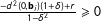 $\frac{-d^{2}(0,\mathbf{b}_{i})(1+\unicode[STIX]{x1D6FF})+r}{1-\unicode[STIX]{x1D6FF}^{2}}\geqslant 0$
or equivalently
 $r\geqslant d^{2}(0,\mathbf{b}_{i})(1+\unicode[STIX]{x1D6FF})$
then ensures that none of the parties, when at the opposition, wants to stay out of the elections. This concludes the proof of parts 1 and 2.
To prove part 4 of the proposition, take the SSMPE
 $\hat{k}_{1}^{\ast }=1$
and
 $\hat{k}_{2}^{\ast }=\frac{1+\unicode[STIX]{x1D6FF}\cos \unicode[STIX]{x1D6FC}}{1+\unicode[STIX]{x1D6FF}}$
and
 $b_{1}\geqslant b_{2}$
, so that
 $\hat{k}_{1}^{\ast }b_{1}\geqslant \hat{k}_{2}^{\ast }b_{2}$
. Starting from
 $\mathbf{q}\in X$
such that
 $k_{2}(\mathbf{q})\leqslant \hat{k}_{2}^{\ast }$
,
 $k_{2}(\mathbf{q})b_{2}=k_{1}(\mathbf{q})b_{1}\leqslant \hat{k}_{2}^{\ast }b_{2}\leqslant \hat{k}_{1}^{\ast }b_{1}$
, both parties run with
 $k_{i}(\mathbf{q})\mathbf{b}_{i}$
when at the opposition in the first period. Since
 $d(k_{i}(\mathbf{q})\mathbf{b}_{i})=d(\mathbf{q})$
, the incumbent’s policy commitment at the beginning of the second period is a policy at the same distance from the origin as
 $\mathbf{q}$
. Thus both parties run with
 $k_{i}(\mathbf{q})\mathbf{b}_{i}$
when at the opposition in the second period. The same holds in any future period. Starting from
 $\mathbf{q}\in X$
such that
 $k_{2}(\mathbf{q})\geqslant \hat{k}_{2}^{\ast }$
, if party
 $2$
is at the opposition in the first period it runs with
 $\hat{k}_{2}^{\ast }\mathbf{b}_{2}$
and if party
 $1$
is at the opposition it runs with
 $\min \{k_{1}(\mathbf{q}),\hat{k}_{1}^{\ast }\}\mathbf{b}_{1}$
. In the former case, the incumbent’s policy commitment at the beginning of the second period satisfies
 $k_{2}(\hat{k}_{2}^{\ast }\mathbf{b}_{2})=\hat{k}_{2}^{\ast }$
, so that the policies alternate on
 $k_{2}(\hat{k}_{2}^{\ast }\mathbf{b}_{2})\mathbf{b}_{2}=\hat{k}_{2}^{\ast }\mathbf{b}_{2}$
and
 $k_{1}(\hat{k}_{2}^{\ast }\mathbf{b}_{2})\mathbf{b}_{1}$
starting from period 2. In the latter case, because
 $k_{2}(\min \{k_{1}(\mathbf{q}),\hat{k}_{1}^{\ast }\}\mathbf{b}_{1})=\min \{k_{1}(\mathbf{q}),\hat{k}_{1}^{\ast }\}\frac{b_{1}}{b_{2}}=\min \{k_{2}(\mathbf{q}),\hat{k}_{1}^{\ast }\frac{b_{1}}{b_{2}}\}\geqslant \hat{k}_{2}^{\ast }$
, party
 $2$
in the second period runs with
 $\hat{k}_{2}^{\ast }\mathbf{b}_{2}$
and the same alternation obtains from period 3 onwards.☐
Proof of Lemma 1
In the SSMPE from Proposition 1, the opposition party
 $i\in \{1,2\}$
contests elections and wins with policy
 $\mathbf{p}_{i}(\mathbf{q})$
, for any incumbent’s policy commitment
 $\mathbf{q}\in X$
. Because
 $u_{v}(\mathbf{x})=-d^{2}(\mathbf{x})$
is decreasing in
 $d(\mathbf{x})$
for any
 $\mathbf{x}\in X$
and
 $d(\mathbf{p}_{i}(\mathbf{q}))=\min \{k_{i}(\mathbf{q}),\hat{k}_{i}\}b_{i}$
for any
 $\mathbf{q}\in X$
, all we have to show is that
 $\min \{k_{i}(\mathbf{q}),\hat{k}_{i}\}b_{i}$
is nondecreasing in
 $\hat{k}_{2}$
,
 $b_{1}$
and
 $b_{2}$
for all
 $i\in \{1,2\}$
and
 $\mathbf{q}\in X$
and is increasing in
 $\hat{k}_{2}$
,
 $b_{1}$
and
 $b_{2}$
for some
 $i\in \{1,2\}$
and
 $\mathbf{q}\in X$
. The nondecreasing part is immediate. For the increasing part, we have
 $\min \{k_{1}(\mathbf{q}),\hat{k}_{1}\}b_{1}=\hat{k}_{1}b_{1}$
when
 $k_{1}(\mathbf{q})>\hat{k}_{1}$
, which is increasing in
 $b_{1}$
because
 $\hat{k}_{1}=1$
, and
 $\min \{k_{2}(\mathbf{q}),\hat{k}_{2}\}b_{2}=\hat{k}_{2}b_{2}$
when
 $k_{2}(\mathbf{q})>\hat{k}_{2}$
, which is increasing in
 $\hat{k}_{2}$
and
 $b_{2}$
because
 $b_{2}>0$
and
 $\hat{k}_{2}=\frac{1+\unicode[STIX]{x1D6FF}\cos \unicode[STIX]{x1D6FC}}{1+\unicode[STIX]{x1D6FF}}>0$
for any
 $\unicode[STIX]{x1D6FC}\in [0,\unicode[STIX]{x1D70B}]$
and
 $\unicode[STIX]{x1D6FF}\in [0,1)$
.☐
Proof of Proposition 3
By Proposition 1,
 $\hat{k}_{1}=1$
and
 $\hat{k}_{2}=\frac{1+\unicode[STIX]{x1D6FF}\cos \unicode[STIX]{x1D6FC}}{1+\unicode[STIX]{x1D6FF}}$
. Notice that
 $\hat{k}_{2}\in (0,1]$
for any
 $\unicode[STIX]{x1D6FF}\in [0,1)$
and
 $\unicode[STIX]{x1D6FC}\in [0,\unicode[STIX]{x1D70B}]$
. To show part 1, using the transformation of polar coordinated to Cartesian ones —
 $\hat{k}_{2}\mathbf{b}_{2}=(\hat{k}_{2}b_{2}\cos \unicode[STIX]{x1D6FC},\hat{k}_{2}b_{2}\sin \unicode[STIX]{x1D6FC})$
—
 $d_{p}$
can be expressed as
 $d_{p}=2b_{2}\hat{k}_{2}\sin {\textstyle \frac{\unicode[STIX]{x1D6FC}}{2}}$
.
 $d_{p}$
is clearly nondecreasing in
 $b_{2}$
, increasing in
 $b_{2}$
when
 $\unicode[STIX]{x1D6FC}>0$
and constant in
 $b_{1}$
. To show part 2,
 $$\begin{eqnarray}\frac{\unicode[STIX]{x2202}\left[2b_{2}{\textstyle \frac{1+\unicode[STIX]{x1D6FF}\cos \unicode[STIX]{x1D6FC}}{1+\unicode[STIX]{x1D6FF}}}\sin {\textstyle \frac{\unicode[STIX]{x1D6FC}}{2}}\right]}{\unicode[STIX]{x2202}\unicode[STIX]{x1D6FC}}=\frac{b_{2}\cos {\textstyle \frac{\unicode[STIX]{x1D6FC}}{2}}}{1+\unicode[STIX]{x1D6FF}}\left[1-2\unicode[STIX]{x1D6FF}+3\unicode[STIX]{x1D6FF}\cos \unicode[STIX]{x1D6FC}\right]\end{eqnarray}$$
where the first term is positive unless
 $\unicode[STIX]{x1D6FC}=\unicode[STIX]{x1D70B}$
. Solving
 $1-2\unicode[STIX]{x1D6FF}+3\unicode[STIX]{x1D6FF}\cos \unicode[STIX]{x1D6FC}=0$
gives
 $\unicode[STIX]{x1D6FC}=\arccos \left[\frac{2\unicode[STIX]{x1D6FF}-1}{3\unicode[STIX]{x1D6FF}}\right]$
. From
 $\{x|\arccos x\in \mathbb{R}\}=[-1,1]$
,
 $-1\leqslant \frac{2\unicode[STIX]{x1D6FF}-1}{3\unicode[STIX]{x1D6FF}}\leqslant 1$
holds when
 $\unicode[STIX]{x1D6FF}\geqslant \frac{1}{5}$
. Because
 $\arccos x\in [0,\unicode[STIX]{x1D70B})$
for
 $x\in (-1,1]$
,
 $\arccos \left[\frac{2\unicode[STIX]{x1D6FF}-1}{3\unicode[STIX]{x1D6FF}}\right]<\unicode[STIX]{x1D70B}$
when
 $\unicode[STIX]{x1D6FF}>\frac{1}{5}$
. Defining
 $\unicode[STIX]{x1D6FC}^{\prime }=\arccos \left[\frac{2\unicode[STIX]{x1D6FF}-1}{3\unicode[STIX]{x1D6FF}}\right]$
when
 $\unicode[STIX]{x1D6FF}\geqslant \frac{1}{5}$
and
 $\unicode[STIX]{x1D6FC}^{\prime }=\unicode[STIX]{x1D70B}$
when
 $\unicode[STIX]{x1D6FF}\in [0,\frac{1}{5})$
,
 $\unicode[STIX]{x1D6FC}^{\prime }<\unicode[STIX]{x1D70B}$
when
 $\unicode[STIX]{x1D6FF}>\frac{1}{5}$
. That
 $d_{p}$
is increasing in
 $\unicode[STIX]{x1D6FC}$
when
 $\unicode[STIX]{x1D6FC}\in [0,\unicode[STIX]{x1D6FC}^{\prime }]$
and decreasing in
 $\unicode[STIX]{x1D6FC}$
when
 $\unicode[STIX]{x1D6FC}\in [\unicode[STIX]{x1D6FC}^{\prime },\unicode[STIX]{x1D70B}]$
then follows from the fact that
 $\cos \unicode[STIX]{x1D6FC}$
, and hence
 $1-2\unicode[STIX]{x1D6FF}+3\unicode[STIX]{x1D6FF}\cos \unicode[STIX]{x1D6FC}$
, is decreasing in
 $\unicode[STIX]{x1D6FC}$
.☐
Appendix B. Extensions
B.1 Model with general utility functions
The model analyzed in this section is identical to the one in the main part of the paper except for the stage utility player
 $i\in \{1,2,v\}$
derives from policy
 $\mathbf{p}$
which now is
 $$\begin{eqnarray}u_{i}(\mathbf{p})=f(d(\mathbf{p},\mathbf{b}_{i}))\end{eqnarray}$$
where
 $f:[0,\infty )\rightarrow \mathbb{R}$
is a continuous, decreasing and concave function in
 $d(\mathbf{p},\mathbf{b}_{i})$
. We also assume that
 $f$
is twice continuously differentiable on
 $(0,\infty )$
. Notice that these assumptions allow
 $f^{\prime }(0)=0$
and
 $f(x)=-x^{2}$
, so that the model in the paper is a special case of the model analyzed here.
For space considerations, we refrain from repeating the arguments leading to Proposition 1 and stress only those aspects of the analysis that differ considerably. An argument similar to the one from the proof of Proposition 1 shows that, since parties use simple strategies, it is (i) optimal for
 $i\in \{1,2\}$
to contest elections with policies located only on the
 $\mathbf{b}_{i}$
-ray and (ii) optimal for
 $v$
to vote for the opposition party running with
 $\mathbf{p}$
when the incumbent’s policy commitment is
 $\mathbf{q}$
if and only if
 $d(\mathbf{p})\leqslant d(\mathbf{q})$
.
In an SSMPE, the extent of moderation of party
 $i\in \{1,2\}$
is the
 $k$
which maximizes
 $\tilde{U} _{i}(k)$
where, for
 $k\geqslant 0$
,
 $$\begin{eqnarray}\begin{array}{@{}ll@{}}\tilde{U} _{i}(k) & \displaystyle =u_{i}(k\mathbf{b}_{i})+u_{i}(kb_{ir}\mathbf{b}_{-i})\unicode[STIX]{x1D6FF}\\ & \displaystyle =f(d(k\mathbf{b}_{i},\mathbf{b}_{i}))+f(d(kb_{ir}\mathbf{b}_{-i},\mathbf{b}_{i}))\unicode[STIX]{x1D6FF}.\\ \end{array}\end{eqnarray}$$
 $\tilde{U} _{i}(k)$
is the dynamic utility party
 $i$
receives, devoid of any constant terms, when it runs with policy
 $k\mathbf{b}_{i}$
and party
 $-i$
, not moderating to a larger extent, runs with
 $kb_{ir}\mathbf{b}_{-i}$
, where we are using the shorthand
 $b_{ir}=\frac{b_{i}}{b_{-i}}$
. The derivation of
 $\tilde{U} _{i}(k)$
is similar to the derivation of (A 6) and is not repeated here.
Condition B1 (Non trivial model).
 $\unicode[STIX]{x1D6FF}\in (0,1)$
and
 $\unicode[STIX]{x1D6FC}\neq 0$
.
Condition B2 (Preserving concavity).
If
 $\unicode[STIX]{x1D6FC}=\unicode[STIX]{x1D70B}$
, then
 $f^{\prime \prime }<0$
.Footnote
23
Condition B3 (Concavity at origin).
 $f^{\prime }(0)>f^{\prime }(b_{i}\sqrt{2(1-\cos \unicode[STIX]{x1D6FC})})\unicode[STIX]{x1D6FF}\sin \frac{\unicode[STIX]{x1D6FC}}{2}$
for
 $i\in \{1,2\}$
.
Lemma B1.
 $\tilde{U} _{i}(k)$
is:
1. continuous and twice continuously differentiable for
$k\neq 1$
;2. increasing for
$k\in [0,\cos \unicode[STIX]{x1D6FC}]$
;3. decreasing for
$k\geqslant 1$
;4. if Conditions B1 and B2 hold, strictly concave for
$k\in (\max \{0,\cos \unicode[STIX]{x1D6FC}\},1)$
;5. if Condition B1 fails, increasing for
$k\in (\max \{0,\cos \unicode[STIX]{x1D6FC}\},1)$
;6. if Condition B2 fails, increasing for
$k\in (0,1)$
.





Proof. The continuity in part 1 follows from the continuity of
 $f$
,
 $d(k\mathbf{b}_{i},\mathbf{b}_{i})$
and
 $d(kb_{ir}\mathbf{b}_{-i},\mathbf{b}_{i})$
. The differentiability follows from the derivatives below, which can be easily checked
 $$\begin{eqnarray}\begin{array}{@{}llll@{}}d(k\mathbf{b}_{i},\mathbf{b}_{i}) & \displaystyle =b_{i}|1-k| & \quad d(kb_{ir}\mathbf{b}_{-i},\mathbf{b}_{i}) & \displaystyle =b_{i}\sqrt{(k-\cos \unicode[STIX]{x1D6FC})^{2}+\sin ^{2}\unicode[STIX]{x1D6FC}}\\ d^{\prime }(k\mathbf{b}_{i},\mathbf{b}_{i}) & \left\{\begin{array}{@{}ll@{}}{<}0\quad & \text{if }k\in [0,1)\\ \nexists \quad & \text{if }k=1\\ {>}0\quad & \text{if }k\in (1,\infty )\end{array}\right. & \quad d^{\prime }(kb_{ir}\mathbf{b}_{-i},\mathbf{b}_{i}) & \left\{\begin{array}{@{}ll@{}}{<}0\quad & \text{if }k<\cos \unicode[STIX]{x1D6FC}\\ =0\quad & \text{if }k=\cos \unicode[STIX]{x1D6FC}\wedge \unicode[STIX]{x1D6FC}\neq 0\\ \nexists \quad & \text{if }k=\cos \unicode[STIX]{x1D6FC}\wedge \unicode[STIX]{x1D6FC}=0\\ {>}0\quad & \text{if }k>\cos \unicode[STIX]{x1D6FC}\end{array}\right.\\ d^{\prime \prime }(k\mathbf{b}_{i},\mathbf{b}_{i}) & \left\{\begin{array}{@{}ll@{}}=0\quad & \text{if }k\neq 1\\ \nexists \quad & \text{if }k=1\end{array}\right. & \quad d^{\prime \prime }(kb_{ir}\mathbf{b}_{-i},\mathbf{b}_{i}) & \left\{\begin{array}{@{}ll@{}}{>}0\quad & \text{if }\unicode[STIX]{x1D6FC}\notin \{0,\unicode[STIX]{x1D70B}\}\\ 0\quad & \text{if }\begin{array}{@{}l@{}}\unicode[STIX]{x1D6FC}=\unicode[STIX]{x1D70B}\,\vee \\ (k\neq 1\wedge \unicode[STIX]{x1D6FC}=0)\end{array}\\ \nexists \quad & \text{if }k=1\wedge \unicode[STIX]{x1D6FC}=0.\end{array}\right.\\ \end{array}\end{eqnarray}$$
 $$\begin{eqnarray}\tilde{U} _{i}^{\prime }(k)=f^{\prime }(d(k\mathbf{b}_{i},\mathbf{b}_{i}))d^{\prime }(k\mathbf{b}_{i},\mathbf{b}_{i})+f^{\prime }(d(kb_{ir}\mathbf{b}_{-i},\mathbf{b}_{i}))d^{\prime }(kb_{ir}\mathbf{b}_{-i},\mathbf{b}_{i})\unicode[STIX]{x1D6FF}\end{eqnarray}$$
and direct verification shows that
 $\tilde{U} _{i}^{\prime }(k)>0$
for
 $k<\cos \unicode[STIX]{x1D6FC}$
,
 $\lim _{k\rightarrow \cos \unicode[STIX]{x1D6FC}^{-}}\tilde{U} _{i}^{\prime }(k)\geqslant 0$
,
 $\tilde{U} _{i}^{\prime }(k)<0$
for
 $k>1$
and
 $\lim _{k\rightarrow 1^{+}}\tilde{U} _{i}^{\prime }(k)\leqslant 0$
.
For the strict concavity for
 $k\in (\max \{0,\cos \unicode[STIX]{x1D6FC}\},1)$
in part 4, we have
 $$\begin{eqnarray}\displaystyle \tilde{U} _{i}^{\prime \prime }(k) & = & \displaystyle f^{\prime \prime }(d(k\mathbf{b}_{i},\mathbf{b}_{i}))\left[d^{\prime }(k\mathbf{b}_{i},\mathbf{b}_{i})\right]^{2}+f^{\prime }(d(k\mathbf{b}_{i},\mathbf{b}_{i}))d^{\prime \prime }(k\mathbf{b}_{i},\mathbf{b}_{i})\nonumber\\ \displaystyle & & \displaystyle +\,\unicode[STIX]{x1D6FF}f^{\prime \prime }(d(kb_{ir}\mathbf{b}_{-i},\mathbf{b}_{i}))\left[d^{\prime }(kb_{ir}\mathbf{b}_{-i},\mathbf{b}_{i})\right]^{2}+f^{\prime }(d(kb_{ir}\mathbf{b}_{-i},\mathbf{b}_{i}))d^{\prime \prime }(kb_{ir}\mathbf{b}_{-i},\mathbf{b}_{i})\unicode[STIX]{x1D6FF}.\end{eqnarray}$$
 $\tilde{U} _{i}^{\prime \prime }(k)\leqslant 0$
is a consequence of the fact that all the summands of the expression are nonpositive. To see that
 $\tilde{U} _{i}^{\prime \prime }(k)<0$
under Conditions B1 and B2, note that the last summand is either zero (when
 $d^{\prime \prime }(kb_{ir}\mathbf{b}_{-i},\mathbf{b}_{i})=0\Rightarrow \unicode[STIX]{x1D6FC}=\unicode[STIX]{x1D70B}$
), which implies that the next to last summand is negative (
 $\unicode[STIX]{x1D6FC}=\unicode[STIX]{x1D70B}\Rightarrow f^{\prime \prime }<0$
by Condition B2), or negative.
For part 5, which claims that
 $\tilde{U} _{i}(k)$
is increasing on
 $(\max \{0,\cos \unicode[STIX]{x1D6FC}\},1)$
when Condition B1 fails, notice that the failure of the condition implies either
 $\unicode[STIX]{x1D6FF}=0$
or
 $\unicode[STIX]{x1D6FC}=0$
. In the latter case the
 $(\max \{0,\cos \unicode[STIX]{x1D6FC}\},1)$
interval is empty so assume
 $\unicode[STIX]{x1D6FF}=0$
and
 $\unicode[STIX]{x1D6FC}>0$
. Substituting
 $\unicode[STIX]{x1D6FF}=0$
into (B 2) gives
 $\tilde{U} _{i}(k)=f(d(k\mathbf{b}_{i},\mathbf{b}_{i}))$
so that
 $\tilde{U} _{i}(k)$
is increasing on
 $(\max \{0,\cos \unicode[STIX]{x1D6FC}\},1)$
. Finally, when Condition B2 in part 6 fails, we have
 $\unicode[STIX]{x1D6FC}=\unicode[STIX]{x1D70B}$
and
 $f^{\prime \prime }=0$
so that
 $d^{\prime }(k\mathbf{b}_{i},\mathbf{b}_{i})=-d^{\prime }(kb_{ir}\mathbf{b}_{-i},\mathbf{b}_{i})=-b_{i}$
for
 $k\in (0,1)$
. This implies that
 $\tilde{U} _{i}^{\prime }(k)=(1-\unicode[STIX]{x1D6FF})c$
where
 $c>0$
so that
 $\tilde{U} _{i}(k)$
is increasing on
 $(0,1)$
.☐
Proposition B1 (SSMPE with General Utility).
When the stage utility of
 $i\in \{1,2,v\}$
is
 $u_{i}(\mathbf{p})=f(d(\mathbf{p},\mathbf{b}_{i}))$
where
 $f$
is a twice continuously differentiable, decreasing and concave function, then:
1. if Condition B1 fails,
$\hat{k}_{1}=\hat{k}_{2}=1$
characterize the unique SSMPE;2. if Condition B2 fails,
$\hat{k}_{1}=\hat{k}_{2}=1$
characterize the unique SSMPE;3. if Conditions B1 and B2 hold, there exists a unique
$\unicode[STIX]{x1D705}_{i}$
for
$i\in \{1,2\}$
given by
$\unicode[STIX]{x1D705}_{i}=\operatorname{argmax}_{k\geqslant 0}\tilde{U} _{i}(k)\in [\max \{0,\cos \unicode[STIX]{x1D6FC}\},1]$
and either
$\unicode[STIX]{x1D705}_{i}b_{i}>\unicode[STIX]{x1D705}_{-i}b_{-i}$
, in which case
$\hat{k}_{i}=1$
and
$\hat{k}_{-i}=\unicode[STIX]{x1D705}_{-i}$
characterize the unique SSMPE, or
$\unicode[STIX]{x1D705}_{1}b_{1}=\unicode[STIX]{x1D705}_{2}b_{2}$
, in which case there exist exactly two SSMPE characterized by
$\hat{k}_{1}=1$
,
$\hat{k}_{2}=\unicode[STIX]{x1D705}_{2}$
and
$\hat{k}_{1}=\unicode[STIX]{x1D705}_{1}$
,
$\hat{k}_{2}=1$
.





Proof. When Condition B1 fails, either
 $\unicode[STIX]{x1D6FF}=0$
or
 $\unicode[STIX]{x1D6FC}=0$
, so that none of the players has any incentive to moderate. By Lemma B1 there exists a unique maximizer of
 $\tilde{U} _{i}(k)$
for
 $i\in \{1,2\}$
,
 $k=1$
, and using arguments similar to the proof of Proposition 1, there exists a unique SSMPE characterized in part 1 of the proposition. When Condition B2 fails, then by Lemma B1 the maximizer of
 $\tilde{U} _{i}(k)$
is
 $k=1$
for
 $i\in \{1,2\}$
. Repeating the same argument just made, there exists a unique SSMPE characterized in part 2 of the proposition.
When both Conditions B1 and B2 hold in part 3, the uniqueness of
 $\unicode[STIX]{x1D705}_{i}=\operatorname{argmax}_{k\geqslant 0}\tilde{U} _{i}(k)$
and
 $\unicode[STIX]{x1D705}_{i}\in [\max \{0,\cos \unicode[STIX]{x1D6FC}\},1]$
follows from Lemma B1. Recalling again the proof of Proposition 1, uniqueness/multiplicity of a SSMPE and its characterization follows.Footnote
24
☐
Proposition B2 (SSMPE Comparative Static with General Utility).
Assume Conditions B1, B2 and B3 hold. Then
 $\unicode[STIX]{x1D705}_{i}\in (\max \{0,\cos \unicode[STIX]{x1D6FC}\},1)$
for
 $i\in \{1,2\}$
in Proposition B1 and (assuming
 $\unicode[STIX]{x1D6FC}\neq \unicode[STIX]{x1D70B}$
for the first relation)
 $$\begin{eqnarray}\frac{\unicode[STIX]{x2202}\unicode[STIX]{x1D705}_{i}}{\unicode[STIX]{x2202}\unicode[STIX]{x1D6FC}}<0\quad \frac{\unicode[STIX]{x2202}\unicode[STIX]{x1D705}_{i}}{\unicode[STIX]{x2202}\unicode[STIX]{x1D6FF}}<0.\end{eqnarray}$$
Proof. From Proposition B1, if Conditions B1 and B2 hold,
 $\unicode[STIX]{x1D705}_{i}=\operatorname{argmax}_{k\geqslant 0}\tilde{U} _{i}(k)\in [\max \{0,\cos \unicode[STIX]{x1D6FC}\},1]$
for
 $i\in \{1,2\}$
. We need to show that Condition B3 implies
 $\unicode[STIX]{x1D705}_{i}\in (\max \{0,\cos \unicode[STIX]{x1D6FC}\},1)$
for
 $i\in \{1,2\}$
. We show that Condition B3 is required only for
 $\unicode[STIX]{x1D705}_{i}<1$
and that
 $\unicode[STIX]{x1D705}_{i}>\max \{0,\cos \unicode[STIX]{x1D6FC}\}$
holds in general. Fix
 $i\in \{1,2\}$
. By Lemma B1 part 4,
 $\tilde{U} _{i}(k)$
is strictly concave for
 $k\in (\max \{0,\cos \unicode[STIX]{x1D6FC}\},1)$
. To show that
 $\unicode[STIX]{x1D705}_{i}<1$
, it thus suffices to show that
 $\lim _{k\rightarrow 1^{-}}\tilde{U} _{i}^{\prime }(k)<0$
. Substituting
 $$\begin{eqnarray}\begin{array}{@{}rclrcl@{}}\displaystyle \lim _{k\rightarrow 1^{-}}(d(k\mathbf{b}_{i},\mathbf{b}_{i})) & = & 0 & \quad \displaystyle \lim _{k\rightarrow 1^{-}}(d^{\prime }(k\mathbf{b}_{i},\mathbf{b}_{i})) & = & -b_{i}\\ \displaystyle \lim _{k\rightarrow 1^{-}}(d(kb_{ir}\mathbf{b}_{-i},\mathbf{b}_{i})) & = & b_{i}\sqrt{2(1-\cos \unicode[STIX]{x1D6FC})} & \quad \displaystyle \lim _{k\rightarrow 1^{-}}(d^{\prime }(kb_{ir}\mathbf{b}_{-i},\mathbf{b}_{i})) & = & b_{i}\sin {\textstyle \frac{\unicode[STIX]{x1D6FC}}{2}}\end{array}\end{eqnarray}$$
into (B 3) gives
 $\lim _{k\rightarrow 1^{-}}\tilde{U} _{i}^{\prime }(k)=-b_{i}[f^{\prime }(0)-f^{\prime }(b_{i}\sqrt{2(1-\cos \unicode[STIX]{x1D6FC})})\unicode[STIX]{x1D6FF}\sin \frac{\unicode[STIX]{x1D6FC}}{2}]<0$
, where the inequality follows from Condition B3. To show that
 $\unicode[STIX]{x1D705}_{i}>\max \{0,\cos \unicode[STIX]{x1D6FC}\}$
, it suffices to show that
 $\lim _{k\rightarrow 0^{+}}\tilde{U} _{i}^{\prime }(k)>0$
when
 $\unicode[STIX]{x1D6FC}\geqslant \frac{\unicode[STIX]{x1D70B}}{2}$
and
 $\lim _{k\rightarrow \cos \unicode[STIX]{x1D6FC}^{+}}\tilde{U} _{i}^{\prime }(k)>0$
when
 $\unicode[STIX]{x1D6FC}<\frac{\unicode[STIX]{x1D70B}}{2}$
. When
 $\unicode[STIX]{x1D6FC}\geqslant \frac{\unicode[STIX]{x1D70B}}{2}$
, substituting
 $$\begin{eqnarray}\begin{array}{@{}rclrcl@{}}\displaystyle \lim _{k\rightarrow 0^{+}}(d(k\mathbf{b}_{i},\mathbf{b}_{i})) & = & b_{i} & \quad \displaystyle \lim _{k\rightarrow 0^{+}}(d^{\prime }(k\mathbf{b}_{i},\mathbf{b}_{i})) & = & -b_{i}\\ \displaystyle \lim _{k\rightarrow 0^{+}}(d(kb_{ir}\mathbf{b}_{-i},\mathbf{b}_{i})) & = & b_{i} & \quad \displaystyle \lim _{k\rightarrow 0^{+}}(d^{\prime }(kb_{ir}\mathbf{b}_{-i},\mathbf{b}_{i})) & = & -b_{i}\cos \unicode[STIX]{x1D6FC}\end{array}\end{eqnarray}$$
into (B 3) gives
 $\lim _{k\rightarrow 0^{+}}\tilde{U} _{i}^{\prime }(k)=-b_{i}f^{\prime }(b_{i})(1+\unicode[STIX]{x1D6FF}\cos \unicode[STIX]{x1D6FC})>0$
. When
 $\unicode[STIX]{x1D6FC}<\frac{\unicode[STIX]{x1D70B}}{2}$
, substituting
 $$\begin{eqnarray}\begin{array}{@{}rclrcl@{}}\displaystyle \lim _{k\rightarrow \cos \unicode[STIX]{x1D6FC}^{+}}(d(k\mathbf{b}_{i},\mathbf{b}_{i})) & = & b_{i}(1-\cos \unicode[STIX]{x1D6FC}) & \quad \displaystyle \lim _{k\rightarrow \cos \unicode[STIX]{x1D6FC}^{+}}(d^{\prime }(k\mathbf{b}_{i},\mathbf{b}_{i})) & = & -b_{i}\\ \displaystyle \lim _{k\rightarrow \cos \unicode[STIX]{x1D6FC}^{+}}(d(kb_{ir}\mathbf{b}_{-i},\mathbf{b}_{i})) & = & b_{i}\sin \unicode[STIX]{x1D6FC} & \quad \displaystyle \lim _{k\rightarrow \cos \unicode[STIX]{x1D6FC}^{+}}(d^{\prime }(kb_{ir}\mathbf{b}_{-i},\mathbf{b}_{i})) & = & 0\end{array}\end{eqnarray}$$
into (B 3) gives
 $\lim _{k\rightarrow \cos \unicode[STIX]{x1D6FC}^{+}}\tilde{U} _{i}^{\prime }(k)=-b_{i}f^{\prime }(b_{i}(1-\cos \unicode[STIX]{x1D6FC}))>0$
.
Since
 $\unicode[STIX]{x1D705}_{i}\in (\max \{0,\cos \unicode[STIX]{x1D6FC}\},1)$
under the conditions of the proposition, it is implicitly defined by
 $\tilde{U} _{i}^{\prime }(\unicode[STIX]{x1D705}_{i})=0$
. From the implicit function theorem
 $\frac{\unicode[STIX]{x2202}\unicode[STIX]{x1D705}_{i}}{\unicode[STIX]{x2202}x}=\frac{\frac{\unicode[STIX]{x2202}}{\unicode[STIX]{x2202}x}\tilde{U} _{i}^{\prime }(\unicode[STIX]{x1D705}_{i})}{-\tilde{U} _{i}^{\prime \prime }(\unicode[STIX]{x1D705}_{i})}$
. The denominator of this expression is positive by strict concavity of
 $\tilde{U} _{i}(k)$
. The numerator of this expression for
 $x\in \{\unicode[STIX]{x1D6FC},\unicode[STIX]{x1D6FF}\}$
is
 $$\begin{eqnarray}\begin{array}{@{}rcl@{}}{\textstyle \frac{\unicode[STIX]{x2202}}{\unicode[STIX]{x2202}\unicode[STIX]{x1D6FC}}}\tilde{U} _{i}^{\prime }(\unicode[STIX]{x1D705}_{i}) & = & f^{\prime \prime }(d(\unicode[STIX]{x1D705}_{i}b_{ir}\mathbf{b}_{-i},\mathbf{b}_{i}))d^{\prime }(\unicode[STIX]{x1D705}_{i}b_{ir}\mathbf{b}_{-i},\mathbf{b}_{i}){\displaystyle \frac{\unicode[STIX]{x2202}d(\unicode[STIX]{x1D705}_{i}b_{ir}\mathbf{b}_{-i},\mathbf{b}_{i})}{\unicode[STIX]{x2202}\unicode[STIX]{x1D6FC}}}\unicode[STIX]{x1D6FF}\\ & & +\,f^{\prime }(d(\unicode[STIX]{x1D705}_{i}b_{ir}\mathbf{b}_{-i},\mathbf{b}_{i})){\displaystyle \frac{\unicode[STIX]{x2202}d^{\prime }(\unicode[STIX]{x1D705}_{i}b_{ir}\mathbf{b}_{-i},\mathbf{b}_{i})}{\unicode[STIX]{x2202}\unicode[STIX]{x1D6FC}}}\unicode[STIX]{x1D6FF}\\ {\textstyle \frac{\unicode[STIX]{x2202}}{\unicode[STIX]{x2202}\unicode[STIX]{x1D6FF}}}\tilde{U} _{i}^{\prime }(\unicode[STIX]{x1D705}_{i}) & = & f^{\prime }(d(\unicode[STIX]{x1D705}_{i}b_{ir}\mathbf{b}_{-i},\mathbf{b}_{i}))d^{\prime }(\unicode[STIX]{x1D705}_{i}b_{ir}\mathbf{b}_{-i},\mathbf{b}_{i})\end{array}\end{eqnarray}$$
where both expressions are negative since
 $\frac{\unicode[STIX]{x2202}}{\unicode[STIX]{x2202}\unicode[STIX]{x1D6FC}}d(\unicode[STIX]{x1D705}_{i}b_{ir}\mathbf{b}_{-i},\mathbf{b}_{i})=\frac{b_{i}\unicode[STIX]{x1D705}_{i}\sin \unicode[STIX]{x1D6FC}}{\sqrt{(\unicode[STIX]{x1D705}_{i}-\cos \unicode[STIX]{x1D6FC})^{2}+\sin ^{2}\unicode[STIX]{x1D6FC}}}>0$
and
 $\frac{\unicode[STIX]{x2202}}{\unicode[STIX]{x2202}\unicode[STIX]{x1D6FC}}d^{\prime }(\unicode[STIX]{x1D705}_{i}b_{ir}\mathbf{b}_{-i},\mathbf{b}_{i})=\frac{b_{i}\sin \unicode[STIX]{x1D6FC}(1-\unicode[STIX]{x1D705}_{i}\cos \unicode[STIX]{x1D6FC})}{\left(\sqrt{(\unicode[STIX]{x1D705}_{i}-\cos \unicode[STIX]{x1D6FC})^{2}+\sin ^{2}\unicode[STIX]{x1D6FC}}\right)^{3}}>0$
.Footnote
25
☐
B.2 Forward-looking representative voter
In this section, we study a version of the model from the main part of the paper in which the representative voter is forward-looking. We will show that for any SSMPE identified in Proposition 1, there exists an equilibrium with forward-looking
 $v$
and that this equilibrium generates a comparative static on the representative voter’s welfare with respect to antagonism and extremism which is identical to the one stated in Corollary 1.
Throughout this section assume
 $\unicode[STIX]{x1D6FF}_{v}\in [0,1)$
. The model from the main part requires the following changes. The utility
 $v$
derives from a sequence of policies
 $\mathbf{P}=\{\mathbf{p}_{0},\mathbf{p}_{1},\ldots \}$
is the discounted sum of payoffs from each period
 $$\begin{eqnarray}U_{v}(\mathbf{P})=\mathop{\sum }_{t=0}^{\infty }\unicode[STIX]{x1D6FF}_{v}^{t}u_{v}(\mathbf{p}_{t}).\end{eqnarray}$$
Given a path of policies generated by play according to
 $\unicode[STIX]{x1D70E}=(\unicode[STIX]{x1D70E}_{1},\unicode[STIX]{x1D70E}_{2},\unicode[STIX]{x1D70E}_{v})$
starting from an incumbent
 $j\in \{1,2\}$
committed to
 $\mathbf{q}$
,
 $\mathbf{P}(\,j,\unicode[STIX]{x1D70E},\mathbf{q})=\{\mathbf{p}_{0},\mathbf{p}_{1},\ldots \}$
, the dynamic utility of
 $v$
is
 $$\begin{eqnarray}V_{v}^{j}(\mathbf{q}|\unicode[STIX]{x1D70E})=U_{v}(\mathbf{P}(\,j,\unicode[STIX]{x1D70E},\mathbf{q}))=\mathop{\sum }_{t=0}^{\infty }\unicode[STIX]{x1D6FF}_{v}^{t}u_{v}(\mathbf{p}_{t}).\end{eqnarray}$$
In Definition 2 of SMPE, we now require
 $\unicode[STIX]{x1D70E}_{v}^{\ast }(\,j,\mathbf{q},\mathbf{p})=\mathit{Yes}$
if and only if
 $$\begin{eqnarray}u_{v}(\mathbf{p})+\unicode[STIX]{x1D6FF}_{v}V_{v}^{i}(\mathbf{p}|\unicode[STIX]{x1D70E}^{\ast })\geqslant u_{v}(\mathbf{q})+\unicode[STIX]{x1D6FF}_{v}V_{v}^{j}(\mathbf{q}|\unicode[STIX]{x1D70E}^{\ast })\end{eqnarray}$$
for any incumbent
 $j\in \{1,2\}$
committed to
 $\mathbf{q}\in X$
and the opposition
 $i=\{1,2\}\setminus \{j\}$
contesting elections with
 $\mathbf{p}\in X$
. Given a profile of strategies
 $\unicode[STIX]{x1D70E}$
, assuming the initial incumbent’s policy commitment
 $\mathbf{q}^{0}$
is distributed according to
 $F(\mathbf{q}^{0})$
with strictly positive density on
 $X$
, and denoting with
 $\unicode[STIX]{x1D70C}\in (0,1)$
the probability that party
 $1$
is the first-period incumbent, the representative voter’s ex ante welfare from the dynamic electoral competition game with parties’ extremism
 $b_{1}$
and
 $b_{2}$
and antagonism
 $\unicode[STIX]{x1D6FC}$
is
 $$\begin{eqnarray}W(b_{1},b_{2},\unicode[STIX]{x1D6FC}|\unicode[STIX]{x1D70E})=\int _{X}\unicode[STIX]{x1D70C}V_{v}^{1}(\mathbf{z}|\unicode[STIX]{x1D70E})+(1-\unicode[STIX]{x1D70C})V_{v}^{2}(\mathbf{z}|\unicode[STIX]{x1D70E})d(F(\mathbf{z})).\end{eqnarray}$$
Proposition B3. For any SSMPE
 $\unicode[STIX]{x1D70E}^{\prime }$
in the model with
 $\unicode[STIX]{x1D6FF}_{v}=0$
identified in Proposition 1, there exists an SMPE
 $\unicode[STIX]{x1D70E}^{\ast }$
in the model with
 $\unicode[STIX]{x1D6FF}_{v}\in (0,1)$
such that:
1. in
$\unicode[STIX]{x1D70E}^{\ast }$
, elections are always contested and incumbents always defeated;2. starting from
$\mathbf{q}\in X$
, policies converge to identical alternation under
$\unicode[STIX]{x1D70E}^{\prime }$
and
$\unicode[STIX]{x1D70E}^{\ast }$
;3.
$W(b_{1},b_{2},\unicode[STIX]{x1D6FC}|\unicode[STIX]{x1D70E}^{\ast })$
is nondecreasing in
$\unicode[STIX]{x1D6FC}$
; increasing in
$\unicode[STIX]{x1D6FC}$
if
$\unicode[STIX]{x1D6FF}>0$
; decreasing in
$b_{i}$
for
$i\in \{1,2\}$
.


Proof. Fix the SSMPE
 $\unicode[STIX]{x1D70E}^{\prime }=(\unicode[STIX]{x1D70E}_{1}^{\prime },\unicode[STIX]{x1D70E}_{2}^{\prime },\unicode[STIX]{x1D70E}_{v}^{\prime })$
from Proposition 1. We construct an SMPE
 $\unicode[STIX]{x1D70E}^{\ast }=(\unicode[STIX]{x1D70E}_{1}^{\ast },\unicode[STIX]{x1D70E}_{2}^{\ast },\unicode[STIX]{x1D70E}_{v}^{\ast })$
for the model with
 $\unicode[STIX]{x1D6FF}_{v}\in [0,1)$
and then show that it possesses the properties from parts 1 through 3. Assume that
 $\unicode[STIX]{x1D70E}^{\prime }$
is such that party
 $2$
moderates, that is
 $\unicode[STIX]{x1D70E}_{1}^{\prime }(\mathbf{q})=\mathbf{p}_{1}(\mathbf{q})$
with
 $\hat{k}_{1}=1$
and
 $\unicode[STIX]{x1D70E}_{2}^{\prime }(\mathbf{q})=\mathbf{p}_{2}(\mathbf{q})$
with
 $\hat{k}_{2}=\frac{1+\unicode[STIX]{x1D6FF}\cos \unicode[STIX]{x1D6FC}}{1+\unicode[STIX]{x1D6FF}}$
for any
 $\mathbf{q}\in X$
. For the ‘mirror’ SSMPE identified in Proposition 1 part 2, the proof is similar and omitted.Footnote
26
Denote
 $\tilde{k}_{2}=\sqrt{\left(\frac{b_{1}}{b_{2}}\right)^{2}(1-\unicode[STIX]{x1D6FF}_{v})+\unicode[STIX]{x1D6FF}_{v}\hat{k}_{2}^{2}}$
and note that, because
 $\hat{k}_{2}\leqslant 1$
and
 $\frac{b_{1}}{b_{2}}\geqslant 1$
,
 $\hat{k}_{2}\leqslant \tilde{k}_{2}\leqslant \frac{b_{1}}{b_{2}}$
. For any
 $\mathbf{q}\in X$
define
 $$\begin{eqnarray}\tilde{p}_{1}(\mathbf{q})=\left\{\begin{array}{@{}ll@{}}k_{1}(\mathbf{q})\quad & \text{for }k_{2}(\mathbf{q})\leqslant \hat{k}_{2}\\ k_{1}(\mathbf{q})\sqrt{{\displaystyle \frac{1-\unicode[STIX]{x1D6FF}_{v}\left({\displaystyle \frac{\hat{k}_{2}b_{2}}{d(\mathbf{q})}}\right)^{2}}{1-\unicode[STIX]{x1D6FF}_{v}}}}\quad & \text{for }k_{2}(\mathbf{q})\in (\hat{k}_{2},\tilde{k}_{2})\\ 1\quad & \text{for }k_{2}(\mathbf{q})\geqslant \tilde{k}_{2}.\end{array}\right.\end{eqnarray}$$
Standard arguments show that
 $\tilde{p}_{1}(\mathbf{x})=\tilde{p}_{1}(\mathbf{y})$
for any
 $\mathbf{x}\in X$
and
 $\mathbf{y}\in X$
if
 $d(\mathbf{x})=d(\mathbf{y})$
and that
 $\tilde{p}_{1}(\mathbf{x})$
is continuous in
 $d(\mathbf{x})$
and increasing in
 $d(\mathbf{x})$
if
 $k_{2}(\mathbf{x})\in [0,\tilde{k}_{2}]$
.
We now construct
 $\unicode[STIX]{x1D70E}^{\ast }$
. For party
 $2$
set
 $\unicode[STIX]{x1D70E}_{2}^{\ast }=\unicode[STIX]{x1D70E}_{2}^{\prime }$
, that is
 $\unicode[STIX]{x1D70E}_{2}^{\ast }$
is a simple strategy
 $\mathbf{p}_{2}$
from Definition 3 with
 $\hat{k}_{2}=\frac{1+\unicode[STIX]{x1D6FF}\cos \unicode[STIX]{x1D6FC}}{1+\unicode[STIX]{x1D6FF}}$
. For party
 $1$
and any
 $\mathbf{q}\in X$
, set
 $\unicode[STIX]{x1D70E}_{1}^{\ast }(\mathbf{q})=\tilde{p}_{1}(\mathbf{q})\mathbf{b}_{1}$
and note that
 $\unicode[STIX]{x1D70E}_{1}^{\ast }=\unicode[STIX]{x1D70E}_{1}^{\prime }$
when
 $\unicode[STIX]{x1D6FF}_{v}=0$
. For
 $v$
set
 $\unicode[STIX]{x1D70E}_{v}^{\ast }$
such that
 $\unicode[STIX]{x1D70E}_{v}^{\ast }(\,j,\mathbf{q},\mathbf{p})=\mathit{Yes}$
if and only if, when
 $j=1$
 $$\begin{eqnarray}\begin{array}{@{}llll@{}}d(\mathbf{p}) & {\leqslant}d(\mathbf{q}) & \quad \text{for }k_{2}(\mathbf{q}) & {\leqslant}\hat{k}_{2}\\ d(\mathbf{p}) & {\leqslant}\sqrt{d^{2}(\mathbf{q})(1-\unicode[STIX]{x1D6FF}_{v})+\unicode[STIX]{x1D6FF}_{v}(\hat{k}_{2}b_{2})^{2}} & \quad \text{for }k_{2}(\mathbf{q}) & \in (\hat{k}_{2},{\textstyle \frac{b_{1}}{b_{2}}})\\ d(\mathbf{p}) & {\leqslant}\sqrt{d^{2}(\mathbf{q})-\unicode[STIX]{x1D6FF}_{v}b_{1}^{2}+\unicode[STIX]{x1D6FF}_{v}(\hat{k}_{2}b_{2})^{2}} & \quad \text{for }k_{2}(\mathbf{q}) & {\geqslant}{\textstyle \frac{b_{1}}{b_{2}}}\end{array}\end{eqnarray}$$
and when
 $j=2$
 $$\begin{eqnarray}\begin{array}{@{}rclll@{}}d(\mathbf{p}) & {\leqslant} & d(\mathbf{q}) & & \quad \text{for }k_{2}(\mathbf{q})\leqslant \hat{k}_{2}\\ d(\mathbf{p}) & {\leqslant} & \tilde{p}_{1}(\mathbf{q})b_{1} & & \quad \text{for }k_{2}(\mathbf{q})\in (\hat{k}_{2},\tilde{k}_{2})\\ d(\mathbf{p}) & {\leqslant} & \sqrt{d^{2}(\mathbf{q})+\unicode[STIX]{x1D6FF}_{v}b_{1}^{2}-\unicode[STIX]{x1D6FF}_{v}(\hat{k}_{2}b_{2})^{2}} & & \quad \text{for }k_{2}(\mathbf{q})\geqslant \tilde{k}_{2}\end{array}\end{eqnarray}$$
and note that
 $\unicode[STIX]{x1D70E}_{v}^{\ast }=\unicode[STIX]{x1D70E}_{v}^{\prime }$
when
 $\unicode[STIX]{x1D6FF}_{v}=0$
.
We now argue that
 $\unicode[STIX]{x1D70E}^{\ast }=(\unicode[STIX]{x1D70E}_{1}^{\ast },\unicode[STIX]{x1D70E}_{2}^{\ast },\unicode[STIX]{x1D70E}_{v}^{\ast })$
constitutes an SMPE. From (B 15) and
 $\unicode[STIX]{x1D70E}_{2}^{\ast }(\mathbf{q})=\min \{k_{2}(\mathbf{q}),\hat{k}_{2}\}\mathbf{b}_{2}$
, party
 $2$
contests and wins elections for any policy commitment
 $\mathbf{q}\in X$
of party
 $1$
. From (B 16) and
 $\unicode[STIX]{x1D70E}_{1}^{\ast }(\mathbf{q})=\tilde{p}_{1}(\mathbf{q})\mathbf{b}_{1}$
, party
 $1$
contests and wins elections for any policy commitment
 $\mathbf{q}\in X$
of party
 $2$
. Because elections are always contested and incumbents always defeated in
 $\unicode[STIX]{x1D70E}^{\prime }$
as well as in
 $\unicode[STIX]{x1D70E}^{\ast }$
, because
 $\unicode[STIX]{x1D70E}_{2}^{\ast }(\mathbf{q})=\unicode[STIX]{x1D70E}_{2}^{\prime }(\mathbf{q})$
and
 $k_{2}(\unicode[STIX]{x1D70E}_{2}^{\ast }(\mathbf{q}))\leqslant \hat{k}_{2}$
for any
 $\mathbf{q}\in X$
and because
 $\unicode[STIX]{x1D70E}_{1}^{\ast }(\mathbf{q})=\unicode[STIX]{x1D70E}_{1}^{\prime }(\mathbf{q})$
for any
 $\mathbf{q}\in X$
such that
 $k_{2}(\mathbf{q})\leqslant \hat{k}_{2}$
, it follows that
 $V_{1}^{1}(\mathbf{q}|\unicode[STIX]{x1D70E}^{\ast })=V_{1}^{1}(\mathbf{q}|\unicode[STIX]{x1D70E}^{\prime })$
for any
 $\mathbf{q}\in X$
and
 $V_{2}^{2}(\mathbf{q}|\unicode[STIX]{x1D70E}^{\ast })=V_{2}^{2}(\mathbf{q}|\unicode[STIX]{x1D70E}^{\prime })$
for any
 $\mathbf{q}\in X$
such that
 $k_{2}(\mathbf{q})\leqslant \hat{k}_{2}$
. In addition, because
 $\tilde{p}_{1}(\mathbf{q})\geqslant k_{1}(\mathbf{q})$
for any
 $\mathbf{q}\in X$
such that
 $k_{2}(\mathbf{q})\leqslant \frac{b_{1}}{b_{2}}$
and because
 $\tilde{p}_{1}(\mathbf{q})=\hat{k}_{1}=1$
for any
 $\mathbf{q}\in X$
such that
 $k_{2}(\mathbf{q})\geqslant \frac{b_{1}}{b_{2}}$
, it follows that
 $V_{2}^{2}(\mathbf{q}|\unicode[STIX]{x1D70E}^{\ast })\leqslant V_{2}^{2}(\mathbf{q}|\unicode[STIX]{x1D70E}^{\prime })$
for any
 $\mathbf{q}\in X$
such that
 $k_{2}(\mathbf{q})>\hat{k}_{2}$
.
From the proof of Proposition 1 we know that
 $u_{1}(k\mathbf{b}_{1})+\unicode[STIX]{x1D6FF}V_{1}^{1}(k\mathbf{b}_{1}|\unicode[STIX]{x1D70E}^{\prime })$
is increasing in
 $k$
for
 $k\in [0,1]$
and decreasing in
 $k$
for
 $k\geqslant 1$
. Since
 $V_{1}^{1}(k\mathbf{b}_{1}|\unicode[STIX]{x1D70E}^{\ast })=V_{1}^{1}(k\mathbf{b}_{1}|\unicode[STIX]{x1D70E}^{\prime })$
for any
 $k\in \mathbb{R}_{{\geqslant}0}$
,
 $\unicode[STIX]{x1D70E}_{1}^{\ast }$
is optimal for party
 $1$
. For a policy commitment
 $\mathbf{q}\in X$
of party
 $2$
such that
 $k_{2}(\mathbf{q})\leqslant \tilde{k}_{2}$
, the largest policy on the
 $\mathbf{b}_{1}$
-ray that generates a victory of party
 $1$
is
 $\tilde{p}_{1}(\mathbf{q})\mathbf{b}_{1}$
, and the same policy maximizes the dynamic utility of party
 $1$
. For a policy commitment
 $\mathbf{q}\in X$
of party
 $2$
such that
 $k_{2}(\mathbf{q})>\tilde{k}_{2}$
, running with policy
 $\mathbf{b}_{1}$
guarantees the electoral victory for party
 $1$
, and the same policy maximizes the dynamic utility of party
 $1$
.
From the proof of Proposition 1 we know that
 $u_{2}(k\mathbf{b}_{2})+\unicode[STIX]{x1D6FF}V_{2}^{2}(k\mathbf{b}_{2}|\unicode[STIX]{x1D70E}^{\prime })$
is increasing in
 $k$
for
 $k\in [0,\hat{k}_{2}]$
and decreasing in
 $k$
for
 $k\geqslant \hat{k}_{2}$
. Since
 $V_{2}^{2}(k\mathbf{b}_{2}|\unicode[STIX]{x1D70E}^{\ast })=V_{2}^{2}(k\mathbf{b}_{2}|\unicode[STIX]{x1D70E}^{\prime })$
for
 $k\in [0,\hat{k}_{2}]$
and
 $V_{2}^{2}(k\mathbf{b}_{2}|\unicode[STIX]{x1D70E}^{\ast })\leqslant V_{2}^{2}(k\mathbf{b}_{2}|\unicode[STIX]{x1D70E}^{\prime })$
for
 $k>\hat{k}_{2}$
,
 $\unicode[STIX]{x1D70E}_{2}^{\ast }$
is optimal for party
 $2$
. For a policy commitment
 $\mathbf{q}\in X$
of party
 $1$
such that
 $k_{2}(\mathbf{q})\leqslant \hat{k}_{2}$
, the largest policy on the
 $\mathbf{b}_{2}$
-ray that generates the victory of party
 $2$
is
 $k_{2}(\mathbf{q})\mathbf{b}_{2}$
, and the same policy maximizes the dynamic utility of party
 $2$
. For a policy commitment
 $\mathbf{q}\in X$
of party
 $1$
such that
 $k_{2}(\mathbf{q})>\hat{k}_{2}$
, running with policy
 $\hat{k}_{2}\mathbf{b}_{2}$
guarantees the electoral victory for party
 $2$
, and the same policy maximizes the dynamic utility of party
 $2$
.
It remains is to be shown that
 $\unicode[STIX]{x1D70E}_{v}^{\ast }$
satisfies the definition of SMPE. From the definition, for any incumbent
 $j\in \{1,2\}$
committed to
 $\mathbf{q}\in X$
and the opposition
 $i=\{1,2\}\setminus \{j\}$
contesting elections with
 $\mathbf{p}\in X$
,
 $\unicode[STIX]{x1D70E}_{v}^{\ast }(\,j,\mathbf{q},\mathbf{p})=\mathit{Yes}$
if and only if
 $$\begin{eqnarray}u_{v}(\mathbf{p})+\unicode[STIX]{x1D6FF}_{v}V_{v}^{i}(\mathbf{p}|\unicode[STIX]{x1D70E}^{\ast })\geqslant u_{v}(\mathbf{q})+\unicode[STIX]{x1D6FF}_{v}V_{v}^{j}(\mathbf{q}|\unicode[STIX]{x1D70E}^{\ast }).\end{eqnarray}$$
Using
 $\unicode[STIX]{x1D70E}_{1}^{\ast }$
,
 $\unicode[STIX]{x1D70E}_{2}^{\ast }$
and
 $u_{v}(\mathbf{q})=-d^{2}(\mathbf{q})$
for any
 $\mathbf{q}\in X$
, straightforward algebra gives
 $$\begin{eqnarray}\begin{array}{@{}ll@{}}V_{v}^{1}(\mathbf{q}|\unicode[STIX]{x1D70E}^{\ast }) & \displaystyle =\left\{\begin{array}{@{}ll@{}}-{\textstyle \frac{d^{2}(\mathbf{q})}{1-\unicode[STIX]{x1D6FF}_{v}}}\quad & \text{ for }k_{2}(\mathbf{q})\leqslant \hat{k}_{2}\\ -{\textstyle \frac{(\hat{k}_{2}b_{2})^{2}}{1-\unicode[STIX]{x1D6FF}_{v}}}\quad & \text{ for }k_{2}(\mathbf{q})>\hat{k}_{2}\end{array}\right.\\ V_{v}^{2}(\mathbf{q}|\unicode[STIX]{x1D70E}^{\ast }) & \displaystyle =\left\{\begin{array}{@{}ll@{}}-{\textstyle \frac{d^{2}(\mathbf{q})}{1-\unicode[STIX]{x1D6FF}_{v}}}\quad & \text{ for }k_{2}(\mathbf{q})\,\leqslant \tilde{k}_{2}\\ -b_{1}^{2}-\unicode[STIX]{x1D6FF}_{v}{\textstyle \frac{(\hat{k}_{2}b_{2})^{2}}{1-\unicode[STIX]{x1D6FF}_{v}}}\quad & \text{ for }k_{2}(\mathbf{q})>\tilde{k}_{2}\end{array}\right.\end{array}\end{eqnarray}$$
which can be used to derive
 $\unicode[STIX]{x1D70E}_{v}^{\ast }$
as stated in (B 15) and (B 16). This concludes the proof that
 $\unicode[STIX]{x1D70E}^{\ast }$
constitutes an SMPE.
Part 1 of the proposition, that elections are always contested and incumbents always defeated under
 $\unicode[STIX]{x1D70E}^{\ast }$
, has already been noted. Part 2 claims that policies converge to identical alternation under
 $\unicode[STIX]{x1D70E}^{\prime }$
and
 $\unicode[STIX]{x1D70E}^{\ast }$
. From Proposition 1, this means alternation between
 $k_{1}(\mathbf{q})\mathbf{b}_{1}$
and
 $k_{2}(\mathbf{q})\mathbf{b}_{2}$
when
 $k_{2}(\mathbf{q})\leqslant \hat{k}_{2}$
and alternation between
 $k_{1}(\hat{k}_{2}\mathbf{b}_{2})\mathbf{b}_{1}$
and
 $\hat{k}_{2}\mathbf{b}_{2}$
when
 $k_{2}(\mathbf{q})>\hat{k}_{2}$
. When
 $k_{2}(\mathbf{q})\leqslant \hat{k}_{2}$
,
 $\unicode[STIX]{x1D70E}^{\ast }$
clearly generates the identical alternation since
 $\unicode[STIX]{x1D70E}_{2}^{\ast }=\unicode[STIX]{x1D70E}_{2}^{\prime }$
and
 $\unicode[STIX]{x1D70E}_{1}^{\ast }(\mathbf{q})=k_{1}(\mathbf{q})\mathbf{b}_{1}$
. When
 $k_{2}(\mathbf{q})>\hat{k}_{2}$
, the first time party
 $2$
contests elections it does so with
 $\unicode[STIX]{x1D70E}_{2}^{\ast }(\mathbf{q})=\hat{k}_{2}\mathbf{b}_{2}$
and from then on the equilibrium policies alternate between
 $k_{1}(\hat{k}_{2}\mathbf{b}_{2})\mathbf{b}_{1}$
and
 $\hat{k}_{2}\mathbf{b}_{2}$
. To show part 3, taking derivatives with respect to
 $\unicode[STIX]{x1D6FC}$
and
 $b_{i}$
for
 $i\in \{1,2\}$
of the expressions in (B 18) shows that
 $\frac{\unicode[STIX]{x2202}}{\unicode[STIX]{x2202}\unicode[STIX]{x1D6FC}}V_{v}^{j}(\mathbf{q}|\unicode[STIX]{x1D70E}^{\ast })\geqslant 0$
and
 $\frac{\unicode[STIX]{x2202}}{\unicode[STIX]{x2202}b_{i}}V_{v}^{j}(\mathbf{q}|\unicode[STIX]{x1D70E}^{\ast })\leqslant 0$
for any
 $i\in \{1,2\}$
, any
 $j\in \{1,2\}$
and any
 $\mathbf{q}\in X$
. At the same time
 $\frac{\unicode[STIX]{x2202}}{\unicode[STIX]{x2202}b_{1}}V_{v}^{2}(\mathbf{q}|\unicode[STIX]{x1D70E}^{\ast })<0$
when
 $k_{2}(\mathbf{q})>\tilde{k}_{2}$
,
 $\frac{\unicode[STIX]{x2202}}{\unicode[STIX]{x2202}b_{2}}V_{v}^{1}(\mathbf{q}|\unicode[STIX]{x1D70E}^{\ast })<0$
when
 $k_{2}(\mathbf{q})>\hat{k}_{2}$
and
 $\frac{\unicode[STIX]{x2202}}{\unicode[STIX]{x2202}\unicode[STIX]{x1D6FC}}V_{v}^{1}(\mathbf{q}|\unicode[STIX]{x1D70E}^{\ast })>0$
when
 $k_{2}(\mathbf{q})>\hat{k}_{2}$
and
 $\unicode[STIX]{x1D6FF}>0$
.☐
B.3 Unique SPE with finite horizon
In this section, we analyze a finite horizon version of the model studied so far. We show that there exists a unique SPE and describe the policy dynamics generated by this equilibrium strategy profile.
Assume the parties compete in
 $T$
consecutive elections, where
 $T<\infty$
. For simplicity, we assume that
 $b_{1}=b_{2}$
and that the two parties have lexicographic preferences over office rents and policy outcomes. This implies that the opposition party, for any incumbent’s policy commitment
 $\mathbf{q}\in X$
, contests the election with a winning policy, if such a policy exists. Denote
 $\unicode[STIX]{x1D705}=\frac{1+\unicode[STIX]{x1D6FF}\cos \unicode[STIX]{x1D6FC}}{1+\unicode[STIX]{x1D6FF}}$
and note that
 $\unicode[STIX]{x1D705}\in (0,1]$
for any
 $\unicode[STIX]{x1D6FF}\in [0,1)$
and
 $\unicode[STIX]{x1D6FC}\in [0,\unicode[STIX]{x1D70B}]$
. We use the notation
 $\mathbf{p}_{i}(\mathbf{q}|\hat{k}_{i})$
for the simple strategies from Definition 3, in order to make explicit their dependence on
 $\hat{k}_{i}$
.
In any SPE, the voting strategy of the representative voter in any period has to satisfy, for any incumbent party
 $j\in \{1,2\}$
, any incumbent’s policy commitment
 $\mathbf{q}\in X$
and any electoral platform of the opposition party
 $\mathbf{p}\in X$
,
 $\unicode[STIX]{x1D70E}_{v}(\,j,\mathbf{q},\mathbf{p})=\mathit{Yes}$
if and only if
 $d(\mathbf{p})\leqslant d(\mathbf{q})$
.
We proceed by backward induction. Consider the last period
 $T$
. For any incumbent’s policy commitment
 $\mathbf{q}\in X$
, the opposition party
 $i$
contests elections with policy
 $\mathbf{p}^{\ast }\in \operatorname{argmax}_{\mathbf{p}\in \{\mathbf{x}\in X|d(\mathbf{x})\leqslant d(\mathbf{q})\}}-d^{2}(\mathbf{p},\mathbf{b}_{i})$
. Clearly,
 $\mathbf{p}^{\ast }$
has to lie on the
 $\mathbf{b}_{i}$
-ray and, hence, can be written as
 $k\mathbf{b}_{i}$
for some
 $k\geqslant 0$
. Denote
 $\tilde{U} _{i,T}(k)=-d^{2}(k\mathbf{b}_{i},\mathbf{b}_{i})$
. Then the optimization problem of party
 $i$
can be written as
 $\max _{k\in [0,k_{i}(\mathbf{q})]}\tilde{U} _{i,T}(k)$
. This problem has a unique solution
 $k=1$
if
 $k_{i}(\mathbf{q})\geqslant 1$
and
 $k=k_{i}(\mathbf{q})$
if
 $k_{i}(\mathbf{q})\leqslant 1$
. In other words,
 $\mathbf{p}_{i}(\mathbf{q}|1)$
is the uniquely optimal strategy of the opposition party
 $i$
for all
 $i\in \{1,2\}$
and
 $\mathbf{q}\in X$
. Denote
 $\mathbf{p}_{i,T}(\mathbf{q})=\mathbf{p}_{i}(\mathbf{q}|1)$
for
 $i\in \{1,2\}$
.
Consider the period
 $T-1$
. For any incumbent’s policy commitment
 $\mathbf{q}\in X$
, the opposition party
 $i$
contests elections with a policy on the
 $\mathbf{b}_{i}$
-ray because both parties use simple strategies in period
 $T$
that depend on
 $d(\mathbf{q})$
but not on the exact location of
 $\mathbf{q}$
. The optimization problem of the opposition party
 $i$
is
 $\max _{k\in [0,k_{i}(\mathbf{q})]}\tilde{U} _{i,T-1}(k)$
where
 $\tilde{U} _{i,T-1}(k)=-d^{2}(k\mathbf{b}_{i},\mathbf{b}_{i})-d^{2}(\mathbf{p}_{-i,T}(k\mathbf{b}_{i}),\mathbf{b}_{i})\unicode[STIX]{x1D6FF}$
. Because
 $\mathbf{p}_{-i,T}(k\mathbf{b}_{i})=k\mathbf{b}_{-i}$
for
 $k\in [0,1]$
and
 $\mathbf{p}_{-i,T}(k\mathbf{b}_{i})=\mathbf{b}_{-i}$
for
 $k\geqslant 1$
,
 $$\begin{eqnarray}\begin{array}{@{}ll@{}}\tilde{U} _{i,T-1}(k) & \displaystyle =-d^{2}(k\mathbf{b}_{i},\mathbf{b}_{i})-d^{2}(k\mathbf{b}_{-i},\mathbf{b}_{i})\unicode[STIX]{x1D6FF}\\ \tilde{U} _{i,T-1}(k) & \displaystyle =-d^{2}(k\mathbf{b}_{i},\mathbf{b}_{i})-d^{2}(\mathbf{b}_{-i},\mathbf{b}_{i})\unicode[STIX]{x1D6FF}\end{array}\end{eqnarray}$$
when
 $k\in [0,1]$
and
 $k\geqslant 1$
, respectively. An identical argument to the one used to prove Lemma A1 then shows that
 $\tilde{U} _{i,T-1}(k)$
has a unique maximum at
 $k=\unicode[STIX]{x1D705}$
, is increasing on
 $[0,\unicode[STIX]{x1D705}]$
and decreasing on
 $[\unicode[STIX]{x1D705},\infty )$
. Thus, the optimization problem of the opposition party
 $i$
has a unique solution
 $k=\unicode[STIX]{x1D705}$
if
 $k_{i}(\mathbf{q})\geqslant \unicode[STIX]{x1D705}$
and
 $k=k_{i}(\mathbf{q})$
if
 $k_{i}(\mathbf{q})\leqslant \unicode[STIX]{x1D705}$
. In other words,
 $\mathbf{p}_{i}(\mathbf{q}|\unicode[STIX]{x1D705})$
is the uniquely optimal strategy of the opposition party
 $i$
for all
 $i\in \{1,2\}$
and
 $\mathbf{q}\in X$
. Denote
 $\mathbf{p}_{i,T-1}(\mathbf{q})=\mathbf{p}_{i}(\mathbf{q}|\unicode[STIX]{x1D705})$
for
 $i\in \{1,2\}$
.
Consider now the period
 $T-2$
. Without repeating the obvious details, for any incumbent’s policy commitment
 $\mathbf{q}\in X$
, the optimization problem of the opposition party
 $i$
writes
 $\max _{k\in [0,k_{i}(\mathbf{q})]}\tilde{U} _{i,T-2}(k)$
where
 $$\begin{eqnarray}\tilde{U} _{i,T-2}(k)=-d^{2}(k\mathbf{b}_{i},\mathbf{b}_{i})-d^{2}(\mathbf{p}_{-i,T-1}(k\mathbf{b}_{i}),\mathbf{b}_{i})\unicode[STIX]{x1D6FF}-d^{2}(\mathbf{p}_{i,T}(\mathbf{p}_{-i,T-1}(k\mathbf{b}_{i})),\mathbf{b}_{i})\unicode[STIX]{x1D6FF}^{2}.\end{eqnarray}$$
Because
 $\mathbf{p}_{-i,T-1}(k\mathbf{b}_{i})=k\mathbf{b}_{-i}$
for
 $k\in [0,\unicode[STIX]{x1D705}]$
and
 $\mathbf{p}_{-i,T-1}(k\mathbf{b}_{i})=\unicode[STIX]{x1D705}\mathbf{b}_{-i}$
for
 $k\geqslant \unicode[STIX]{x1D705}$
, we have
 $\mathbf{p}_{i,T}(\mathbf{p}_{-i,T-1}(k\mathbf{b}_{i}))=k\mathbf{b}_{i}$
if
 $k\in [0,\unicode[STIX]{x1D705}]$
and
 $\mathbf{p}_{i,T}(\mathbf{p}_{-i,T-1}(k\mathbf{b}_{i}))=\unicode[STIX]{x1D705}\mathbf{b}_{i}$
if
 $k\geqslant \unicode[STIX]{x1D705}$
. Hence
 $$\begin{eqnarray}\begin{array}{@{}ll@{}}\tilde{U} _{i,T-2}(k) & \displaystyle =-d^{2}(k\mathbf{b}_{i},\mathbf{b}_{i})-d^{2}(k\mathbf{b}_{-i},\mathbf{b}_{i})\unicode[STIX]{x1D6FF}-d^{2}(k\mathbf{b}_{i},\mathbf{b}_{i})\unicode[STIX]{x1D6FF}^{2}\\ \tilde{U} _{i,T-2}(k) & \displaystyle =-d^{2}(k\mathbf{b}_{i},\mathbf{b}_{i})-d^{2}(\unicode[STIX]{x1D705}\mathbf{b}_{-i},\mathbf{b}_{i})\unicode[STIX]{x1D6FF}-d^{2}(\unicode[STIX]{x1D705}\mathbf{b}_{i},\mathbf{b}_{i})\unicode[STIX]{x1D6FF}^{2}\end{array}\end{eqnarray}$$
when
 $k\in [0,\unicode[STIX]{x1D705}]$
and
 $k\geqslant \unicode[STIX]{x1D705}$
, respectively. We first note that
 $\tilde{U} _{i,T-2}(k)$
is increasing on
 $[0,\unicode[STIX]{x1D705}]$
, which follows from
 $\tilde{U} _{i,T-2}^{\prime }(k)=\tilde{U} _{i,T-1}^{\prime }(k)-2b_{i}^{2}\unicode[STIX]{x1D6FF}^{2}(k-1)>\tilde{U} _{i,T-1}^{\prime }(k)>0$
for any
 $k\in (0,\unicode[STIX]{x1D705})$
. Furthermore,
 $\tilde{U} _{i,T-2}(k)$
is clearly increasing on
 $[\unicode[STIX]{x1D705},1]$
and decreasing on
 $[1,\infty )$
. Thus the optimization problem of the opposition party
 $i$
has a unique solution
 $k=1$
if
 $k_{i}(\mathbf{q})\geqslant 1$
and
 $k=k_{i}(\mathbf{q})$
if
 $k_{i}(\mathbf{q})\leqslant 1$
. In other words,
 $\mathbf{p}_{i}(\mathbf{q}|1)$
is the uniquely optimal strategy of the opposition party
 $i$
for all
 $i\in \{1,2\}$
and
 $\mathbf{q}\in X$
. Denote
 $\mathbf{p}_{i,T-2}(\mathbf{q})=\mathbf{p}_{i}(\mathbf{q}|1)$
for
 $i\in \{1,2\}$
.
Consider the period
 $T-3$
. For any
 $\mathbf{q}\in X$
, the optimization problem of the opposition party
 $i$
writes
 $\max _{k\in [0,k_{i}(\mathbf{q})]}\tilde{U} _{i,T-3}(k)$
, where similar arguments as in the previous period show
 $$\begin{eqnarray}\begin{array}{@{}ll@{}}\tilde{U} _{i,T-3}(k) & \displaystyle =-d^{2}(k\mathbf{b}_{i},\mathbf{b}_{i})-d^{2}(k\mathbf{b}_{-i},\mathbf{b}_{i})\unicode[STIX]{x1D6FF}-d^{2}(k\mathbf{b}_{i},\mathbf{b}_{i})\unicode[STIX]{x1D6FF}^{2}-d^{2}(k\mathbf{b}_{-i},\mathbf{b}_{i})\unicode[STIX]{x1D6FF}^{3}\\ \tilde{U} _{i,T-3}(k) & \displaystyle =-d^{2}(k\mathbf{b}_{i},\mathbf{b}_{i})-d^{2}(k\mathbf{b}_{-i},\mathbf{b}_{i})\unicode[STIX]{x1D6FF}-d^{2}(\unicode[STIX]{x1D705}\mathbf{b}_{i},\mathbf{b}_{i})\unicode[STIX]{x1D6FF}^{2}-d^{2}(\unicode[STIX]{x1D705}\mathbf{b}_{-i},\mathbf{b}_{i})\unicode[STIX]{x1D6FF}^{3}\end{array}\end{eqnarray}$$
when
 $k\in [0,\unicode[STIX]{x1D705}]$
and
 $k\geqslant \unicode[STIX]{x1D705}$
, respectively. Denoting by
 $\unicode[STIX]{x1D710}_{i}(k)=-d^{2}(k\mathbf{b}_{i},\mathbf{b}_{i})-d^{2}(k\mathbf{b}_{-i},\mathbf{b}_{i})\unicode[STIX]{x1D6FF}$
,
 $\tilde{U} _{i,T-3}(k)=(1+\unicode[STIX]{x1D6FF}^{2})\unicode[STIX]{x1D710}_{i}(k)$
if
 $k\in [0,\unicode[STIX]{x1D705}]$
and
 $\tilde{U} _{i,T-3}(k)=\unicode[STIX]{x1D710}_{i}(k)+c$
if
 $k\geqslant \unicode[STIX]{x1D705}$
, where
 $c$
is constant in
 $k$
. Because
 $\unicode[STIX]{x1D710}_{i}(k)$
is increasing in
 $k$
on
 $[0,\unicode[STIX]{x1D705}]$
and decreasing in
 $k$
on
 $[\unicode[STIX]{x1D705},\infty )$
,
 $\tilde{U} _{i,T-3}(k)$
has a unique maximum at
 $k=\unicode[STIX]{x1D705}$
. By the now familiar arguments,
 $\mathbf{p}_{i}(\mathbf{q}|\unicode[STIX]{x1D705})$
is the uniquely optimal strategy of the opposition party
 $i$
for all
 $i\in \{1,2\}$
and
 $\mathbf{q}\in X$
. Denote
 $\mathbf{p}_{i,T-3}(\mathbf{q})=\mathbf{p}_{i}(\mathbf{q}|\unicode[STIX]{x1D705})$
for
 $i\in \{1,2\}$
.
So far, we have shown that it is uniquely optimal for the opposition party
 $i$
to contest elections with
 $\mathbf{p}_{i}(\mathbf{q}|\hat{k}_{i})$
, where
 $\hat{k}_{i}=1$
for
 $T$
and
 $T-2$
and
 $\hat{k}_{i}=\unicode[STIX]{x1D705}$
for
 $T-1$
and
 $T-3$
. Suppose that this patterns repeats for periods up to
 $T-s+2$
and
 $T-s+1$
where
 $s$
is even.
Consider period
 $T-s$
. We need to show that it is uniquely optimal for the opposition party
 $i$
to contest elections with
 $\mathbf{p}_{i}(\mathbf{q}|1)$
for all
 $i\in \{1,2\}$
and
 $\mathbf{q}\in X$
. Because in
 $T-s+1$
the opposition party contests elections with
 $\mathbf{p}_{i}(\mathbf{q}|\unicode[STIX]{x1D705})$
,
 $$\begin{eqnarray}\begin{array}{@{}ll@{}}\tilde{U} _{i,T-s}(k) & \displaystyle =\unicode[STIX]{x1D710}_{i}(k)\mathop{\sum }_{t=0}^{(s-2)/2}\unicode[STIX]{x1D6FF}^{2t}-d^{2}(k\mathbf{b}_{i},\mathbf{b}_{i})\unicode[STIX]{x1D6FF}^{s}\\ \tilde{U} _{i,T-s}(k) & \displaystyle =-d^{2}(k\mathbf{b}_{i},\mathbf{b}_{i})+c\end{array}\end{eqnarray}$$
when
 $k\in [0,\unicode[STIX]{x1D705}]$
and
 $k\geqslant \unicode[STIX]{x1D705}$
, respectively. Because
 $\unicode[STIX]{x1D710}_{i}(k)$
is increasing in
 $k$
on
 $[0,\unicode[STIX]{x1D705}]$
and decreasing in
 $k$
on
 $[\unicode[STIX]{x1D705},\infty )$
, and because
 $-d^{2}(k\mathbf{b}_{i},\mathbf{b}_{i})$
is increasing in
 $k$
on
 $[0,1]$
and decreasing in
 $k$
on
 $[1,\infty )$
,
 $\tilde{U} _{T-s}(k)$
has a unique maximum
 $k=1$
. Hence, it is uniquely optimal for the opposition party
 $i$
to contest elections with
 $\mathbf{p}_{i}(\mathbf{q}|1)$
for all
 $i\in \{1,2\}$
and
 $\mathbf{q}\in X$
.
Consider
 $T-s-1$
. We need to show that it is uniquely optimal for the opposition party
 $i$
to contest elections with
 $\mathbf{p}_{i}(\mathbf{q}|\unicode[STIX]{x1D705})$
for all
 $i\in \{1,2\}$
and
 $\mathbf{q}\in X$
. Because in
 $T-s$
the opposition party contests elections with
 $\mathbf{p}_{i}(\mathbf{q}|1)$
and in
 $T-s+1$
with
 $\mathbf{p}_{i}(\mathbf{q}|\unicode[STIX]{x1D705})$
,
 $$\begin{eqnarray}\begin{array}{@{}ll@{}}\tilde{U} _{i,T-s-1}(k) & \displaystyle =\unicode[STIX]{x1D710}_{i}(k)\mathop{\sum }_{t=0}^{s/2}\unicode[STIX]{x1D6FF}^{2t}\\ \tilde{U} _{i,T-s-1}(k) & \displaystyle =\unicode[STIX]{x1D710}_{i}(k)+c\end{array}\end{eqnarray}$$
when
 $k\in [0,\unicode[STIX]{x1D705}]$
and
 $k\geqslant \unicode[STIX]{x1D705}$
, respectively. Because
 $\unicode[STIX]{x1D710}_{i}(k)$
is increasing in
 $k$
on
 $[0,\unicode[STIX]{x1D705}]$
and decreasing in
 $k$
on
 $[\unicode[STIX]{x1D705},\infty )$
,
 $\tilde{U} _{T-s-1}(k)$
has a unique maximum
 $k=\unicode[STIX]{x1D705}$
. Hence, it is uniquely optimal for the opposition party
 $i$
to contest elections with
 $\mathbf{p}_{i}(\mathbf{q}|\unicode[STIX]{x1D705})$
for all
 $i\in \{1,2\}$
and
 $\mathbf{q}\in X$
.
To summarize, there exists a unique SPE in which the opposition party
 $i$
contests elections with
 $\mathbf{p}_{i}(\mathbf{q}|\hat{k}_{i})$
for all
 $i\in \{1,2\}$
and
 $\mathbf{q}\in X$
.
 $\hat{k}_{i}=1$
for all periods
 $T-s$
with
 $s\in \mathbb{N}_{{\geqslant}0}$
and
 $s$
even and
 $\hat{k}_{i}=\unicode[STIX]{x1D705}$
for all periods
 $T-s$
with
 $s\in \mathbb{N}_{{\geqslant}1}$
and
 $s$
odd. With an appropriately chosen initial-period incumbent party, the SPE just described generates identical policy dynamics to the one generated by the SSMPE from Proposition 1, for any incumbent’s policy commitment
 $\mathbf{q}\in X$
. When party
 $2$
is at the opposition in the initial period of the infinite horizon model, both parties moderate, if at the opposition, in the initial period of the finite horizon model with
 $T$
even. When party
 $1$
is at the opposition in the initial period of the infinite horizon model, none of the parties moderates, if at the opposition, in the initial period of the finite horizon model with
 $T$
odd.