The Baseline Model

The baseline model for our analysis and comparison is the standard crisis bargaining ultimatum game (Fearon Reference Fearon1995), in which two countries dispute a resource of unit size. Country 1 proposes to divide the resource so that it keeps a share $$$x\, \in \,[{\rm{0}},{\rm{1}}]$$$ , leaving 1 − x for the other country. Country 2 can then accept or reject this offer. If accepted, there is a peaceful settlement of the dispute and the payoffs are equal to the shares x and 1 − x. If the proposal is rejected, war occurs. In the case of war, Country 1 wins the resource with a known probability p and Country 2 wins with the complementary probability, 1 − p. To simplify notation, we sometimes write p_i for the probability that Country i wins a conflict, where p ₁ = p and p ₂ = 1 − p. Each side to the dispute pays a cost c_i if war occurs. Thus the expected payoff of war to Country i is p_i − c_i.

It is well known that because war is costly, there is a set of peaceful agreements that both countries would prefer to fighting. In a complete information environment, the probability of the dispute turning to war is 0. In the unique sub-game perfect equilibrium of this crisis bargaining game, Country 1 demands the largest share that Country 2 will accept, which is x* = p + c ₂.

With uncertainty things are more interesting. We consider a model with one-sided incomplete information. We assume that Country 1's cost, c ₁, is common knowledge and that Country 2's cost, c ₂, is private information. To start we also assume that Country 2 can have two possible cost types. Let c ₂ = c_H with probability q and c ₂ = c_L with probability 1 − q, where $$$0\, \lt \,{{c}_L}\, \lt \,{{c}_H}$$$ . We denote the high cost type of Country 2 by 2H and the low cost type of Country 2 by 2L. Later we will extend our results to the case with a continuum of types.

Under these assumptions, the standard model has a unique equilibrium, the nature of which depends on the value of q. We will focus on settings in which the equilibrium produces a positive probability of war. If q > (c_L + c ₁)/(c_H + c ₁), then the proposer demands an equilibrium share x* = p + c_H, the low cost type of Country 2 rejects this proposal and the high cost type of Country 2 accepts. In the two-type case, this equilibrium has a risk-reward trade-off. The proposer is willing to risk war with the low cost type in order to get the better settlement when there is peace with the high cost type.

In what follows, we let q* = (c_L + c ₁)/(c_H + c ₁) and refer to the assumption that q > q* as the screening condition. This is because the equilibrium offer in this case serves to screen the low type from the high type by inducing different responses from each type.

No Commitment to Agreements

In the baseline model with incomplete information, the screening offer generates different responses from the two types. Thus Country 1 learns the true type of Country 2 but is unable to act on this information in the baseline model. We now make the simplest modification to the standard model to allow for the possibility of retractable offers and, with this change, relax the assumed level of commitment to agreements in crisis bargaining.

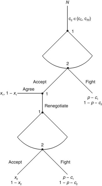
In this new model, illustrated in Figure 1, Country 1 still gets to make an initial offer (x ₁, 1 − x ₁), and if it is rejected the game ends with war. If, however, Country 2 accepts the offer, then Country 1 can agree – obtaining the payoffs (x ₁, 1 − x ₁) – or renegotiate. If Country 1 renegotiates, then it makes a second proposal x ₂ at some future time. This second proposal is a true take-it-or-leave-it offer. As is standard, all payoffs in the second period are discounted by the discount factor $$$\delta \, \in \,({\rm{0,1}}]$$$ . If the second proposal is accepted, then the payoffs for Country 1 and Country 2 are δx ₂ and δ(1 − x ₂). If the second proposal is rejected, then war ensues and its payoff is discounted by δ. So rejection in the first period leads to immediate war, but acceptance can be renegotiated. We therefore label the rejection of an offer as a choice by Country 2 to fight. We refer to this game as G_A.

Fig. 1

Game G_A, with no commitment to agreements

Our equilibrium concept is (strong) perfect Bayesian equilibrium (PBE), as defined by Fudenberg and Tirole (Reference Fudenberg and Tirole1991). The key requirement of this definition is that if Country 1 deviates in the first period by making an off-the-equilibrium-path offer, it must still use Country 2's strategy in response to this offer to calculate its belief (via Bayes’ Rule) in Period 2.

In the model without commitment to agreements, when q > q* and δ < 1, there is a unique (strong) PBE outcome.

Before providing the technical details in support of this result, it is useful to understand the intuition of the result and the implications for learning in crisis bargaining. This result says that even though we permit Country 1 to retract its offer and renegotiate, it chooses not to do so in equilibrium. Specifically, because the low cost type rejects Country 1's initial offer and the high cost type accepts, after observing an acceptance Country 1 knows for sure that it is facing a high cost type. What may be surprising about this result is that even at this point, with all uncertainty resolved, Country 1 does not renegotiate even though it has learned the type of Country 2 with certainty. The reason for this is that Country 1's initial equilibrium offer, x* = p + c_H, is the same as the optimal offer for Country 1 when it knows for sure that it is facing the high cost type of Country 2. Thus there is no incentive for Country 1 to make a different offer in the second period, even after learning the type of country it faces.

We now lay out some useful facts that will aid in our proof of the proposition. We begin our analysis in the second period. Let μ_A(x ₁) denote the belief of Country 1 about the type of Country 2 in the second period after an offer x ₁ in the first period. Specifically, μ_A(x ₁) = P[c ₂ = c_H|x ₁ accepted], the probability that Country 1 believes Country 2 is the high cost type. As Period 2 is just a standard ultimatum game, we know from standard arguments that in every PBE, $$${{x}_2}\, \in \,\{ p\, + \,{{c}_L},p\, + \,{{c}_H}\} $$$ . Moreover, these standard arguments yield x ₂ = p + c_L if μ_A < q*, x ₂ = p + c_H if μ_A > q*, and Country 1 is indifferent between making these two offers if μ_A = q*. Finally, we know from standard arguments that if x ₂ = p + c_L in equilibrium, then both types of Country 2 accept this offer with probability one, and if x ₂ = p + c_H in equilibrium, then 2H accepts with probability one and 2L fights with probability one. Therefore, it is easy to see that whatever value μ_A takes, the (undiscounted) payoff to 2L in Period 2 is 1 − p − c_L. Moreover, the (undiscounted) payoff to 2H is in the interval [1 − p − c_H, 1 − p − c_L]. Likewise, the (undiscounted) payoff to Country 1 is $$$v_{{\rm{1}}}^{\ast} ({{\mu }_A}({{x}_{\rm{1}}}))$$$ , where

$$v_{{\rm{1}}}^{\ast} (\mu )\, = \,\max \{ p\, + \,{{c}_L},\mu (p\, + \,{{c}_H})\, + \,{\rm{(1}}\,{\rm{ - }}\,\mu )(p\,{\rm{ - }}\,{{c}_{\rm{1}}})\} $$

is the equilibrium utility to Country 1 of the one-shot ultimatum game with prior μ.

Let r(x ₁) be the probability that Country 1 chooses to renegotiate after an offer x ₁ has been accepted. As the payoff of renegotiating is no higher than δ(p + c_H) and no lower than δ(p + c_L), it follows that in every equilibrium r(x ₁) = 0 for all x ₁ > δ(p + c_H) and r(x ₁) = 1 for all x ₁ < δ(p + c_L). Our first result is a simple consequence of incentive compatibility.

Proof. In order for accept to be a best response to x ₁ for 2L, we must have:

$$ \displaylines{ &amp; r({{x}_{\rm{1}}})\delta ({{p}_2}{\rm{\, - \, }}{{c}_L})\, + \,({\rm{1\, - \, }}r({{x}_{\rm{1}}}))({\rm{1\, - \, }}{{x}_{\rm{1}}})\,\geq \,{{p}_{\rm{2}}}{\rm{\, - \, }}{{c}_L} \cr &amp; {\rm{(1 \, - \, }}r({{x}_{\rm{1}}}))({\rm{1\, - \, }}{{x}_{\rm{1}}})\,\geq \,({\rm{1\, - \, }}r({{x}_{\rm{1}}})\delta )({{p}_{\rm{2}}}{\rm{\, - \, }}{{c}_L}). \cr} $$

However, the minimum payoff for 2H for accepting is r(x ₁)δ(p ₂ − c_H) + (1 − r(x₁))(1 − x ₁). Therefore 2H must accept with probability one when

$$\displaylines{ &amp; r({{x}_{\rm{1}}})\delta ({{p}_{\rm{2}}}{\rm{\, - \, }}{{c}_H})\, + \,({\rm{1\, - \, }}r({{x}_{\rm{1}}}))({\rm{1\, - \, }}{{x}_{\rm{1}}})\, \gt \,{{p}_{\rm{2}}}{\rm{\, - \, }}{{c}_H} \cr &amp; ({\rm{1\, - \, }}r({{x}_{\rm{1}}}))({\rm{1\, - \, }}{{x}_{\rm{1}}})\, \gt \,({\rm{1\, - \, }}r({{x}_{\rm{1}}})\delta )({{p}_{\rm{2}}}{\rm{\, - \, }}{{c}_H}). \cr}$$

As c_L < c_H, it is clear that the inequality for 2L implies inequality for 2 H. This establishes the lemma. □

So if the low cost type is not fighting for sure, then the high cost type must be accepting for sure. We are now ready to prove the proposition.

Proof. Consider an arbitrary offer x ₁. For 2L, this offer will either be accepted or play will move to Period 2. Therefore accepting this offer will give a payoff no larger than max {l − x ₁, δ(1 − p − c_L)}. It follows that 2L will choose to fight in response to every offer such that 1 − p − c_L > l − x ₁, which is equivalent to x ₁ > p + c_L. For x ₁ < δ(p + c_L) we know that r(x ₁) = 1, and so 2L strictly prefers to fight. For 2H, because r(x ₁) = 0 for all x ₁ > δ(p + c_H), it follows that 2H strictly prefers to fight for all x ₁ > p + c_H and strictly prefers to accept for all x ₁ ∈ (δ(p + c_H), p + c_H). From this, we see that the utility to Country 1 of making an offer x ₁ > p + c_H is p − c ₁. However, for all offers x ₁ ∈ (max {δ(p + c_H), p + c_H}, p + c_H), the above implies that the utility to Country 1 is qx ₁ + (1 − q)(p − c ₁). In particular, this means that Country 1 can achieve a payoff arbitrarily close to q(p + c_H) + (1 − q)(p − c ₁). It follows that it cannot be an equilibrium for Country 1 to make an offer x ₁ > p + c_H. In addition, no offer x ₁ ∈ (max {δ(p + c_H), p + c_L}, p + c_H) can be optimal, as Country 1 can deviate to a slightly higher offer and improve its payoff.

Next we show that it cannot be an equilibrium for Country 1 to offer x ₁ ≤ max {δ(p + c_H), p + c_L}. We consider two cases. First, suppose δ(p + c_H) > p + c_L. Then for all x ₁ ∈ (p + c_L, δ(p + c_H)], 2L is fighting with probability one, so the maximum possible utility to Country 1 is qδ(p + c_H) + (1 − q)(p − c ₁), which cannot be optimal. For x ₁ ≤ p + c_L, if 2L is fighting with probability one then the preceding argument still holds. Otherwise, 2L is accepting with positive probability, which according to Lemma 1 implies that 2H is accepting with probability one and the Country 1 either renegotiates or agrees. If it renegotiates, its highest possible payoff is again qδ(p + c_H) + (1 − q)(p − c ₁), and if it agrees, its highest possible payoff is x ₁ ≤ p + c_L, which, given q > q*, is strictly less than q(p + c_H) + (1 − q)(p − c ₁). So no such offer can be optimal.

The second case is δ(p + c_H) ≤ p + c_L. For all x ₁ ≤ p + c_L, if 2L is fighting with probability one, then the maximum possible utility to Country 1 is q(p + c_L) + (1 − q)(p − c ₁), which cannot be optimal. Otherwise 2L is accepting with positive probability, which according to Lemma 1 implies that 2H is accepting with probability one and that Country 1 either renegotiates or agrees. If it renegotiates, its highest possible payoff is qδ(p + c_H) + (1 − q)(p − c ₁), and if it agrees, its highest possible payoff is x ₁ ≤ p + c_L, which, given q > q*, is strictly less than q(p + c_H) + (1 − q)(p − c ₁). So no such offer can be optimal.

From this we conclude that the only possible equilibrium offer is x ₁ = p + c_H, which 2L rejects and, by standard arguments, 2H accepts with probability one. It is clear that Country 1 will agree with this acceptance. This proves the proposition. □

Although this model's equilibrium path of play is unique, the equilibrium strategies are not unique. In particular, for some offers, several strategies are consistent with equilibrium. For example, suppose δ(p + c_H) > p + c_L and consider the offer x ₁ = δ(p + c_H). From the above, we know that 2L will fight in response to this offer. It is easy to see that it is sequentially rational for 2H to accept this offer and for Country 1 to agree. But there are also mixed strategies that are consistent with equilibrium. As long as 2H accepts with positive probability, Country 1 believes Country 2 is the high type and will offer x ₂ = p + c_H, which Country 1 expects to be accepted. Therefore Country 1 is indifferent between agreeing and renegotiating. Indeed, it is consistent with equilibrium for 2H to accept with probability one and for Country 1 to mix with probability r ≤ p + c_H. In fact, if Country 1 plays r ≤ p + c_H, type 2H is indifferent between accepting and fighting, and it is consistent with equilibrium for 2H to arbitrarily mix between these two choices.

It is also true that, while the equilibrium outcome is the same as for a one-shot ultimatum game, the behavior for non-equilibrium offers can be very different from equilibrium behavior in the ultimatum game. For example, the following is a PBE to this game. Country 1 offers x ₁ = p + c_H, chooses r(x ₁) = 1 for all x ₁ < δ(p + c_H) and r(x ₁) = 0 for all x ₁ ≥ δ(p + c_H), and chooses x ₂(x ₁) = p + c_H for all x ₁. Type 2L fights in response to every x ₁ and type 2H fights in response to every x ₁ < δ(p + c_H) and to every x ₁ > p + c_H and accepts in response to every x ₁ ∈ [δ(p + c_H), p + c_H]. One notable feature of this equilibrium is that 2L rejects all offers and both 2H and 2L reject generous offers (x ₁ < δ(p + c_H)). The intuition for this is that if a generous offer is accepted, Country 1 will not agree (it is too generous!), but renegotiation is always worse for both types than fighting in the first period.

When δ is equal to one, the set of equilibrium outcomes expands. For example, when δ = 1 we can give examples of PBE in which both types of Country 2 choose to fight with probability one and also examples in which the outcome is fighting with some probability and agreement on the one-shot ultimatum offer with the remaining probability. That these kinds of equilibria exist may be surprising, as one could imagine a profitable deviation for the proposer of making a slightly more generous offer, which would typically be accepted with probability one. But with costless renegotiation (due to δ = 1), such an offer by Country 1 is not credible, as Country 1 would renegotiate after acceptance. How big is the set of equilibria when δ = 1? In fact, fighting and agreement on p + c_H are the only possible outcomes that can occur in equilibrium. In other words, there are no strong PBE in which agreement occurs (with positive probability) on an offer other than the one-shot ultimatum offer.

Proof. We must show that if a peaceful agreement is reached with positive probability in equilibrium, then this agreement will be at x = p + c_H. So to begin, take an arbitrary offer x ₁ and assume that it is agreed to with positive probability by some type of Country 2, and that Country 1 chooses renegotiation with positive probability in an equilibrium. (Note that we do not require that x ₁ be the equilibrium offer of Country 1.) We will show that Country 1 will offer x ₂ = p + c_H for sure in the second period. Suppose not; that is, that Country 1 offers x ₂ = p + c_L with positive probability. First, note that if Country 1 chooses renegotiation with positive probability, it must be that x ₁ ≤ p + c_H. Secondly, note that by agreeing to x ₁, type 2H will receive 1 − x ₁ ≥ 1 − p − c_H with probability less than one, when Country 1 chooses to agree, and when Country 1 chooses to renegotiate, receives 1 − p − c_L with positive probability because x ₂ = p + c_L with positive probability by supposition, and 1 − p − c_H with the remaining probability. As this expected utility is strictly greater than 1 − p − c_H, type 2H will agree to x ₁ with probability one. But then by Bayes’ Rule, μ_A(x ₁) ≥ q > q* and so Country 1 will choose x ₂ = p + c_H with certainty in Period 2. This establishes that if agreement is reached with positive probability in the second period, it must be at x = p + c_H.

The only other possibility is that there is agreement in the first period. So suppose $$${{\widetilde{x}}_1}$$$ is the equilibrium offer of Country 1 that is accepted with positive probability by some type of Country 2, and that Country 1 agrees to this acceptance with positive probability. The above result shows that if Country 1 is not agreeing with probability one, then x ₂ = p + c_H will be offered in the second period. From this, we see that if $$${{\widetilde{x}}_1}$$$ is greater than p + c_H, then for both types of Country 2, accepting gives a positive probability of utility $$$1{\rm{\, - \, }}{{\widetilde{x}}_1}$$$ and the remaining probability of utility 1 − p − c_H, which is strictly worse than the utility of fighting for both types. Therefore it must be that $$${{\widetilde{x}}_1}$$$ < p + c_H. However, suppose $$${{\widetilde{x}}_1}$$$ < p + c_H. Then, as acceptance is agreed to with positive probability, it is clear that 2H must be accepting $$${{\widetilde{x}}_1}$$$ with probability one. If $$${{\widetilde{x}}_1}$$$ ∈ (p + c_L, p + c_H), then clearly 2L will choose to fight with probability one in the first period, but then it is optimal for Country 1 to renegotiate with probability one instead of agreeing with positive probability. If $$${{\widetilde{x}}_1}$$$ ≤ p + c_L, then the highest possible payoff of agreeing is p + c_{L ,}which is smaller than the payoff of renegotiating, because Country 1's belief in the second period will be strictly greater than q*. So again, this contradicts the assumption that Country 1 is agreeing with positive probability. We therefore conclude that $$${{\widetilde{x}}_1}$$$ = p + c_H, which concludes the proof.

□

No Commitment to Fighting

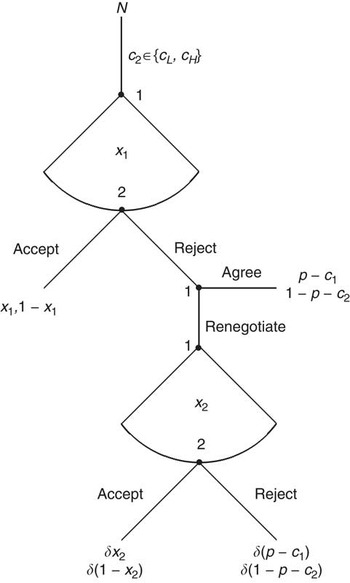
We now examine what happens when we relax the commitment assumptions of the baseline model in a different way. We suppose that agreements are binding, but that rejecting an offer can lead to continued bargaining. Specifically, in this game Country 1 makes an initial offer x ₁ ∈ [0, 1] in Period 1, which Country 2 either accepts or rejects. If Country 2 accepts the offer, then Countries 1 and 2 receive payoffs of x ₁ and 1 − x ₁, respectively. If Country 2 rejects the offer, then Country 1 can either decide to end the bargaining and fight, which gives each side its war payoff (p − c_i), or to move the game to a second period of bargaining, in which the payoff to both sides is discounted by a factor of δ ∈ (0, 1). Specifically, following a rejection by Country 2 in the first period and a decision by Country 1 to continue to the second period, Country 1 makes an offer x ₂ ∈ [0, 1], which Country 2 either accepts or rejects. If Country 2 accepts the offer, then Countries 1 and 2 receive payoffs of δx ₂ and δ(1 − x ₂), respectively. If Country 2 rejects the offer, then war ensues and each Country i receives its (discounted) war payoff, which is given by δ(p_i − c_i). This game, in which agreements are binding but rejections can be renegotiated, is illustrated in Figure 2. We refer to this game as game G_R.

Fig. 2

Game G_R, with no commitment to fighting

Recall that q* = (c ₁ + c_L)/(c ₁ + c_H) and $$$v_{1}^{\ast} (\mu )\, = \,\max \{ p\, + \,{{c}_L},\mu (p\, + \,{{c}_H})\, + \,({\rm{1\, - \, }}\mu )(p{\rm{\, - \, }}{{c}_{\rm{1}}})\} $$$ . We let $$$x_{L}^{\ast} \, = \,{\rm{1\, - \, }}\delta ({\rm{1\, - \, }}p{\rm{\, - \, }}{{c}_L})$$$ and $$$x_{H}^{\ast} \, = \,{\rm{1\, - \, }}\delta ({\rm{1\, - \, }}p{\rm{\, - \, }}{{c}_H})$$$ . It is clear that $$$0\, \lt \,x_{L}^{\ast} \, \lt \,x_{H}^{\ast} \, \lt \,{\rm{1}}$$$ .

We also let

$${{\delta }^\ast} \, = \,\max \left\{ {\frac{{{\rm{1\, - \, }}q}}{{{\rm{1\, - \, }}q\, + (q{\rm{\, - \, }}{{q}^\ast} )({{c}_H}{\rm{\, - \, }}{{c}_L})}},\frac{{p{\rm{\, - \, }}{{c}_{\rm{1}}}}}{{p\, + \,{{c}_L}}}} \right\}.$$

As before, we describe some useful facts about the second period of this game. Let μ_R(x ₁) denote the belief of Country 1 about the type of Country 2 in the second period, after an offer x ₁ in the first period. Specifically, $$${{\mu }_R}({{x}_{\rm{1}}})\, = \,P[{{c}_{\rm{2}}}\, = \,{{c}_H}&#x007C;{{x}_{\rm{1}}}\:\ rejected]$$$ , the probability that Country 1 believes Country 2 is the high cost type. As in the last section, we know that x ₂ = p + c_L if μ_R < q*, x ₂ = p + c_H if μ_R > q* and Country 1 is indifferent between making these two offers if μ_R = q*. Moreover, if x ₂ = p + c_L in equilibrium, then both types of Country 2 accept this offer with probability one, and if x ₂ = p + c_H then 2H accepts with probability one and 2L rejects with probability one. Finally, whatever value μ_R takes, the (undiscounted) payoff to 2L in Period 2 is 1 − p − c_L. Moreover, the (undiscounted) payoff to 2H is in the interval [1 − p − c_H, 1 − p − c_L]. Likewise, the (undiscounted) payoff to Country 1 is $$$v_{{\rm{1}}}^{\ast} ({{\mu }_R}({{x}_{\rm{1}}}))$$$ .

The following proposition characterizes the unique (strong) PBE of this game.

Proof. Consider Country 1's decision after an arbitrary offer x ₁ has been rejected. Given Country 1's belief μ_R(x ₁) at this point in the game, its payoff from continuing to bargain is $$$\delta v_{{\rm{1}}}^{\ast} ({{\mu }_R}({{x}_{\rm{1}}}))\geq \delta (p\, + \,{{c}_L})$$$ . By choosing to fight at this point, however, Country 1 receives a payoff of p − c ₁. Given our condition on δ, we know that δ(p + c_L) > p − c ₁. Therefore it is never optimal for Country 1 to fight after an offer has been rejected. In other words, in every PBE, Country 1 always continues bargaining rather than fighting, regardless of the initial offer x ₁.

Now we turn to Period 1. Consider an arbitrary offer x ₁. For 2L, rejecting this offer gives a payoff of δ(1 − p − c_L). Therefore, 2L will reject any offer such that 1 − x ₁ < δ(1 − p − c_L), which is equivalent to $$${{x}_{\rm{1}}}\, \gt \,x_{L}^{\ast} $$$ , and will accept any offer such that $$${{x}_{\rm{1}}}\, \lt \,x_{L}^{\ast} $$$ . For 2H, because rejecting this offer gives a payoff of at most δ(1 − p − c_L), 2H will also accept any offer such that $$${{x}_1} \lt x_{L}^{\ast} $$$ . On the other hand, because rejecting this offer gives 2H a payoff of at least δ(1 − p − c_H), 2H will reject any offer such that $$${{x}_{\rm{1}}}\, \gt \,x_{H}^{\ast} $$$ . Because both types of Country 2 accept any offer $$${{x}_{\rm{1}}}\,\lt \,x_{L}^{\ast} $$$ , in any PBE the payoff to Country 1 satisfies $$$u_{{\rm{1}}}^{\ast} ({{x}_{\rm{1}}})\, = \,{{x}_{\rm{1}}}$$$ for all $$${{x}_{\rm{1}}}\, \in \,[0,x_{L}^{\ast} )$$$ . An immediate consequence of this is that there is no PBE in which Country 1 makes such an offer with positive probability.

In any strong PBE, the belief of Country 1 must be derived via Bayes’ Rule from the sequentially rational response of Country 2 to a given offer, whether this offer is on or off the equilibrium path. Thus as both types of Country 2 reject any offer $$${{x}_{\rm{1}}}\, \gt \,x_{H}^{\ast} $$$ , in any strong PBE μ_R(x ₁) = q. This implies that in any strong PBE, $$$u_{{\rm{1}}}^{\ast} ({{x}_{\rm{1}}})\, = \,\delta v_{{\rm{1}}}^{\ast} (q)$$$ for all $$${{x}_{\rm{1}}}\, \in \,(x_{H}^{\ast}, {\rm{1}}]$$$ .

Next, consider an offer $$${{x}_{\rm{1}}}\, \in \,(x_{L}^{\ast}, x_{H}^{\ast} )$$$ . From above, 2L rejects this offer. We claim that 2H must play a mixed strategy in response to this offer. If 2H rejects x ₁ with probability one, then μ_R(x ₁) = q and because q > q*, x ₂ = p + c_H. This gives 2H a payoff of $$${\rm{1\, - \, }}x_{H}^{\ast} $$$ . But then deviating to accepting x ₁ gives a payoff strictly greater than $$${\rm{1\, - \, }}x_{H}^{\ast} $$$ , so this cannot be an equilibrium. If 2H accepts x ₁ with probability one, then μ_R(x ₁) = 0 and therefore x ₂ = p + c_L. So deviating to rejecting x ₁ gives a payoff of $$${\rm{1\, - \, }}x_{L}^{\ast} $$$ , which is strictly greater than 1 − x ₁. Therefore this cannot be an equilibrium. So 2H must play a mixed strategy.

In order to calculate this mixed strategy, let s(x ₁) be the probability that 2H accepts $$${{x}_{\rm{1}}}\, \in \,(x_{L}^{\ast}, x_{H}^{\ast} )$$$ . In order to make 2H indifferent between accepting and rejecting x ₁, Country 1 must mix between x ₂ = p + c_L and x ₂ = p + c_H. So let r(x ₁) be the probability that Country 1 makes the offer x ₂ = p + c_L after offering x ₁ in the first period. In order to ensure that 2H is indifferent, we must have

$${\rm{1\, - \, }}{{x}_{\rm{1}}}\, = \,r({{x}_{\rm{1}}})\delta ({\rm{1\, - \, }}p{\rm{\, - \, }}{{c}_L})\, + \,({\rm{1\, - \, }}r({{x}_{\rm{1}}}))\delta ({\rm{1\, - \, }}p{\rm{\, - \, }}{{c}_H}).$$

Solving this linear equation gives the following unique solution:

$$r({{x}_{\rm{1}}})\, = \,\frac{{{\rm{1\, - \, }}\delta ({\rm{1\, - \, }}p{\rm{\, - \, }}{{c}_H}){\rm{\, - \, }}{{x}_{\rm{1}}}}}{{\delta ({{c}_H}{\rm{\, - \, }}{{c}_L})}}\, = \,\frac{{x_{H}^{\ast} {\rm{\, - \, }}{{x}_{\rm{1}}}}}{{\delta ({{c}_H}{\rm{\, - \, }}{{c}_L})}}.$$

In order for Country 1 to be willing to mix in Period 2, it must be indifferent between offering x ₂ = p + c_L and x ₂ = p + c_H. This requires that μ_R = q*. From Bayes’ Rule we know that the belief μ_R is given by

$${{\mu }_R}\, = \,\frac{{q({\rm{1\, - \, }}s({{x}_{\rm{1}}}))}}{{q({\rm{1\, - \, }}s({{x}_{\rm{1}}}))\, + \,({\rm{1\, - \, }}q)}}\, = \,\frac{{q{\rm{\, - \, }}qs({{x}_{\rm{1}}})}}{{{\rm{1\, - \, }}qs({{x}_{\rm{1}}})}},$$

and that this allows us to solve for s(x ₁), which is given by

$$s({{x}_{\rm{1}}})\, = \,\frac{{q{\rm{\, - \, }}{{q}^\ast} }}{{q({\rm{1\, - \, }}{{q}^\ast} )}}.$$

It is easy to see that s(x ₁) ∈ (0, 1) and, in fact, that s(x ₁) is independent of x ₁.

Given this unique mixed strategy, we can calculate the expected utility of Country 1 making an offer $$${{x}_{\rm{1}}}\, \in \,(x_{L}^{\ast}, x_{H}^{\ast} )$$$ . This utility is given by

$$\displaylines{ u_{{\rm{1}}}^{\ast} ({{x}_{\rm{1}}})\, = &amp; \,qs({{x}_{\rm{1}}}){{x}_{\rm{1}}}\, + \,(({\rm{1\, - \, }}q)\, + \,q({\rm{1\, - \, }}s({{x}_{\rm{1}}})))\delta (p\, + \,{{c}_L}) \cr \, = \,\frac{{{{x}_{\rm{1}}}(q{\rm{\, - \, }}{{q}^\ast} )\, + \,\delta ({\rm{1\, - \, }}q)(p\, + \,{{c}_L})}}{{{\rm{1\, - \, }}{{q}^\ast} }}. \cr}$$

As q > q*, we see that $$$u_{{\rm{1}}}^{\ast} ({{x}_{\rm{1}}})$$$ is linearly increasing in x ₁. A direct implication of this is that there is no PBE in which Country 1 puts positive probability on any $$${{x}_{\rm{1}}}\, \in \,(x_{L}^{\ast}, x_{H}^{\ast} )$$$ .

Next, consider an offer $$${{x}_{\rm{1}}}\, \gt \,x_{H}^{\ast} $$$ . As both types of Country 2 will reject this offer, the utility to Country 1 of making this offer is

$$u_{{\rm{1}}}^{\ast} ({{x}_{\rm{1}}})\, = \,\delta v_{{\rm{1}}}^{\ast} (q)\, = \,\delta [({\rm{1\, - \, }}q)(p{\rm{\, - \, }}{{c}_{\rm{1}}})\, + \,q(p\, + \,{{c}_H})].$$

Although we omit the details, it is possible to show algebraically that

$$\frac{{x_{H}^{\ast} (q{\rm{\, - \, }}{{q}^\ast} )\, + \,\delta ({\rm{1\, - \, }}q)(p\, + \,{{c}_L})}}{{{\rm{1\, - \, }}{{q}^\ast} }}{\rm{\, - \, }}u_{{\rm{1}}}^{\ast} ({{x}_{\rm{1}}})\, = \,\frac{{({\rm{1\, - \, }}\delta )(q{\rm{\, - \, }}{{q}^\ast} )}}{{{\rm{1\, - \, }}{{q}^\ast} }}.$$

As q > q*, this shows that there exists a value $$${{x}_{{\rm{1}}^{\prime}}}\, \lt \,x_{H}^{\ast} $$$ that is sufficiently close to $$$x_{H}^{\ast} $$$ that gives Country 1 a payoff strictly greater than $$$u_{{\rm{1}}}^{\ast} ({{x}_{\rm{1}}})$$$ . Therefore there is no PBE in which Country 1 puts positive probability on $$${{x}_{\rm{1}}}\, \gt \,x_{H}^{\ast} $$$ .

By process of elimination, the only two remaining possibilities are $$${{x}_{\rm{1}}}\, = \,x_{L}^{\ast} $$$ and $$${{x}_{\rm{1}}}\, = \,x_{H}^{\ast} $$$ . Consider the offer $$${{x}_{\rm{1}}}\, = \,x_{H}^{\ast} $$$ . Of course, 2L rejects this offer. If Country 1 offers x ₂ = p + c_L in the second period, then 2H will strictly prefer to reject x ₁ as well. This implies μ_R = q > q*, so Country 1 strictly prefers to offer x ₂ = p + c_H. This argument shows that Country 1 must play x ₂ = p + c_H with positive probability after $$${{x}_{\rm{1}}}\, = \,x_{H}^{\ast} $$$ . This requires that $$${{\mu }_R}{\rm{(}}x_{H}^{\ast} {\rm{)}}\,\geq \,{{q}^\ast} $$$ . This in turn implies that the probability that 2H accepts $$${{x}_{\rm{1}}}\, = \,x_{H}^{\ast} $$$ , which is denoted s*, must satisfy $$${{s}^\ast} \,\geq \,(q{\rm{\, - \, }}{{q}^\ast} )/(q({\rm{1\, - \, }}{{q}^\ast} ))$$$ . Moreover, if $$${{x}_{\rm{1}}}\, = \,x_{H}^{\ast} $$$ is played with positive probability in equilibrium, we must have $$$u_{{\rm{1}}}^{\ast} (x_{H}^{\ast} )\,\geq \,u_{{\rm{1}}}^{\ast} ({{x}_{\rm{1}}})$$$ for all $$${{x}_{\rm{1}}}\, \in \,(x_{L}^{\ast}, x_{H}^{\ast} )$$$ . This requires that

$${{s}^\ast} \, = \,\frac{{q{\rm{\, - \, }}{{q}^\ast} }}{{q({\rm{1\, - \, }}{{q}^\ast} )}}.$$

In order for 2H to be indifferent between accepting and rejecting $$${{x}_{\rm{1}}}\, = \,x_{H}^{\ast} $$$ , it must be that x ₂ = p + c_H with probability one. We conclude that

$$u_{{\rm{1}}}^{\ast} (x_{H}^{\ast} )\, = \,\frac{{x_{H}^{\ast} (q{\rm{\, - \, }}{{q}^\ast} )\, + \,\delta ({\rm{1\, - \, }}q)(p\, + \,{{c}_L})}}{{{\rm{1\, - \, }}{{q}^\ast} }}$$

if this offer is played with positive probability. In order for this offer to be an equilibrium, $$$u_{{\rm{1}}}^{\ast} (x_{H}^{\ast} )\,\geq \,u_{{\rm{1}}}^{\ast} ({{x}_{\rm{1}}})$$$ for all $$${{x}_{\rm{1}}}\, \lt \,x_{L}^{\ast} $$$ . As the highest possible payoff from $$${{x}_{\rm{1}}}\, = \,x_{L}^{\ast} $$$ is the limit of $$$u_{{\rm{1}}}^{\ast} ({{x}_{\rm{1}}})$$$ as $$$ {{x}_{\rm{1}}}\, \rightarrow \,x_{L}^{\ast} $$$ , this condition also ensures that there is no profitable deviation to $$${{x}_{\rm{1}}}\, = \,x_{L}^{\ast} $$$ . This condition is satisfied if and only if

$$\frac{{x_{H}^{\ast} (q{\rm{\, - \, }}{{q}^\ast} )\, + \,\delta ({\rm{1\, - \, }}q)(p\, + \,{{c}_L})}}{{{\rm{1\, - \, }}{{q}^\ast} }}\,\geq \,x_{L}^{\ast} $$

Again we omit the details, but this inequality holds when

$$\delta \,\geq \,\frac{{{\rm{1\, - \, }}q}}{{{\rm{1\, - \, }}q\, + \,(q{\rm{\, - \, }}{{q}^\ast} )({{c}_H}{\rm{\, - \, }}{{c}_L})}}\, = \,{{\delta }^\ast} .$$

So for all δ > δ*, there exists a unique strong PBE in which Country 1 makes the offer $$${{x}_{\rm{1}}}\, = \,x_{H}^{\ast} $$$ . □

The key feature of this result is that agreement does not necessarily occur immediately. The high cost type of Country 2 sometimes accepts Country 1's initial offer, and sometimes delays and accepts the offer in the second round. The low cost type of Country 2, on the other hand, rejects both offers and ends up in war, as in the baseline model with commitment. Indeed, although the exact value of the offers made differs from the baseline model, the main intuitions carry over. Country 1 makes demanding offers in both periods and ends up with peaceful agreements with high cost types of Country 2, and war with low cost types. Upon closer examination, we see that the differences, such as they are, are driven by Country 1's ability to delay war until the second period, which lowers the bargaining leverage inherent in rejecting offers. In support of this, we see that as δ goes to one, the offers of Country 1 in both periods converge to the standard screening offer x = p + c_H.

No Commitment to Agreement or Rejection

Finally we consider the case in which there is neither commitment to enact accepted proposals nor to fight when an offer is rejected. In this case, Country 2's choice to either accept or reject can be renegotiated by Country 1. However, we do permit Country 2 to make a third choice of fighting, which cannot be renegotiated by Country 1. We are interested in how the equilibria outcomes of this more general game relate to the equilibria outcomes of the models presented in the earlier sections.

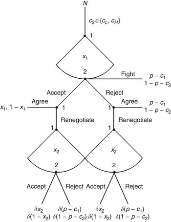
We will denote the version of the game without commitment to agreeing or rejection by G_AR. In this version of the game, Country 1 makes an initial offer x ₁ ∈ [0,1] in Period 1. Country 2 responds by choosing to either accept, reject or fight. If Country 2 chooses to fight, war ensues and both sides receive their war payoff p_i − c_i. If Country 2 accepts the offer, then Country 1 can either agree, in which case the two sides receive payoffs of x ₁ and 1 − x ₁, respectively, or choose to renegotiate, which moves the game to a second round of bargaining. Finally, if Country 2 rejects the offer, then Country 1 can either decide to end the bargaining and fight, which gives each side its war payoff, or to move the game to a second period of bargaining. In the second round, the payoff to both sides is discounted by a factor δ ∈ (0,1). Specifically, Country 1 makes an offer x ₂ ∈ [0,1], which Country 2 either accepts or rejects. If Country 2 accepts the offer, then Countries 1 and 2 receive payoffs of δx ₂ and δ(1 − x ₂), respectively. If Country 2 rejects the offer, then war ensues and each Country i receives its (discounted) war payoff, which is given by δ(p_i − c_i). So in this version of the model, either acceptance or rejection can be countered with a new offer, but fighting leads to immediate war. We illustrate game G_AR in Figure 3. We begin with the following useful lemma:

Fig. 3

Game G_AR, with no commitment

Proof. Let σ* be an equilibrium of G_AR in which after an offer x ₁, some type rejects this offer with positive probability. Let c_m be equal to c_L if this type rejects x ₁ with positive probability, otherwise let c_m be equal to c_H. By standard ultimatum game arguments, in the second period, Country 1 will make an offer to Country 2 that is no smaller than the war payoff of type c_m of Country 2, so that 1 − x ₂ ≤ p ₂ − c_m. So the maximum payoff achievable by type c_m in the second period is δ(p ₂ − c_m). Now, moving back to Country 1's decision on whether to renegotiate or fight after Country 2's rejection, let q_F be the probability that Country 1 fights. Then the utility of type c_m of Country 2 for rejecting is q_F(p ₂ − c_m) + (1 − q_F)δ(p ₂ − c_m). As p ₂ > c_m and δ < 1, this payoff is strictly less than p ₂ − c_m for all q_F < 1. But in order for rejecting to be played with positive probability by type c_m, it must be at least as good as fighting, which gives a payoff of p ₂ − c_m. This establishes that q_F = 1. □

For games G_A and G_AR, the outcome of a strategy profile is a probability distribution over fighting in Periods 1 and 2 and the terms of settlement in Periods 1 and 2. In other words, the outcome is defined over terminal nodes in which all “fight” terminal nodes in a given period are grouped together and all “peaceful settlement” nodes with given terms in a given period are grouped together. Our main result is that, viewed this way, the model with no commitment to either agreement or rejection has the same equilibrium distribution of outcomes as the baseline ultimatum game model.

Proof. As game G_A has a unique distribution of equilibrium outcomes, which is equal to the one-shot ultimatum game, it is enough to show that every equilibrium outcome of G_AR is an equilibrium outcome of G_A. Suppose σ* is an equilibrium of G_AR. We will construct an equilibrium σ′ of G_A that has an identical outcome. To begin, consider an arbitrary offer x ₁ by Country 1 in the first period. If neither type chooses to reject this offer (with positive probability), then the construction of σ′ is simple: it is equal to σ*. As it is optimal for all types to either accept or fight under σ*, it is still optimal for these types to take these same actions when the reject option is unavailable. Clearly, the outcome of G_AR under σ* is identical to the outcome of G_A under σ′.

The other possibility is that some type rejects the offer x ₁ with positive probability. In this case, σ′ is equal to σ* for the type (if any) that does not reject with positive probability and σ′ is equal to the fight action in Period 1 for all types that do reject with positive probability under σ*. To see that σ′ represents equilibrium play, we use Lemma 2 to note that the equilibrium outcome of every type that is rejecting under σ* is fighting in Period 1. Therefore these types receive the same utility under σ′ by choosing to fight instead. For those types that are not rejecting under σ*, since a possible deviation to reject gives the same utility as choosing to fight, there is no change in equilibrium incentives for these types when the reject option is removed. Therefore σ′ represents optimal behavior in G_A. Moreover, the outcome for the types that reject under σ* is fighting in Period 1, and by construction, the outcome in G_A for these types under σ′ is also fighting in Period 1. This shows that the outcome of G_AR under σ* is identical to the outcome of G_A under σ′.

We conclude that for all offers x ₁, the outcome of G_AR under σ* is identical to the outcome of G_A under σ′. Therefore the optimal choice of offer by Country 1 must be the same in σ* and σ′, and so every equilibrium outcome of G_AR is an equilibrium outcome of G_A. □

Results with A Continuum of Types

While the intuition is clear in the two-type case as to why there is no incentive to renegotiate in the short run when there is no commitment to agreements, one might be concerned that the fact that Country 1 can make only one of two proposals in equilibrium is driving the results. Perhaps the presence of more types—and the possibility of a continuum of complete information equilibrium offers—might change the results. Thus in order to see how robust our results are, we next analyze the case with a continuum of cost types.

Suppose c ₂ is distributed according to a differentiable and strictly increasing cumulative distribution function F with support [0,1 − p] and density function f. In the one-shot ultimatum game, it is easy to see that Country 2 will reject an offer x when c ₂ < x − p and accept the offer when c ₂ > x − p. From this, it follows that the utility to Country 1 of making an offer x, which we denote v(x), is given by

$$v(x)\, = \,F(x{\rm{\, - \, }}p)(p{\rm{\, - \, }}{{c}_{\rm{1}}})\, + \,({\rm{1\, - \, }}F(x{\rm{\, - \, }}p))x.$$

The next lemma demonstrates that this function has a unique maximizer and gives a simple condition on when it is interior.

Proof. As the set of possible offers is [0, 1] and v(x) is continuous on this set, a maximizer exists. It is clear from inspection that offering x < p is not optimal. Likewise, it is clear that offering x = 1 is not optimal. Now, the derivative of v(x) can be written as

$$v^{\prime}(x)\, = \,[{\rm{1\, - \, }}F(x{\rm{\, - \, }}p)]\left[ {{\rm{1\, - \, }}h(x{\rm{\, - \, }}p)(x{\rm{\, - \, }}(p{\rm{\, - \, }}{{c}_{\rm{1}}}))} \right],$$

where h(x) = f(x)/(1 − F(x)) is the hazard rate. As h(x − p) is nondecreasing and always positive on [p, 1), and the term x −(p − c ₁) is strictly increasing and always positive on [p, 1), the product of these two terms is strictly increasing on [p, 1).

Now suppose f(0) ≥ 1/c ₁. This is equivalent to h(0)c ₁ ≥ 1, which is equivalent to v′(p) ≤ 0. Moreover, by the above we know that h(x −p)(x −(p − c ₁)) > 1 for all x ∈ (p, 1), so v′(x) < 0 for all such x. This establishes that x* = p is the unique maximizer of v(x) in this case. However, suppose f(0) < 1/c ₁—which is equivalent to v′(p) > 0—so x = p is not a maximizer. Again, as h(x − p)(x − (p − c ₁)) is strictly increasing on (p, 1), this term cannot be equal to 1 for more than one value of x. Therefore, there must exist a unique maximizer x* ∈ (p, 1). This proves the lemma. □

This lemma implies that in the one-shot ultimatum game, there is a unique PBE in which Country 1 offers x* and Country 2 responds to this offer according to the cutpoint c* = x* − p. To avoid boundary cases, we assume throughout this section that f(0) < 1/c ₁, so that the cutpoint c* is interior to the interval [0, 1 − p].

No Commitment to Agreements

We begin with game G_A, in which Country 1 can choose to renegotiate accepted offers. An arbitrary strong PBE can be described by the following: the equilibrium choice of x ₁; for each possible offer x ₁, the cutpoint $$$\hat{c}({{x}_{\rm{1}}})$$$ such that Country 2 rejects x ₁ in the first period if $$${{c}_{\rm{2}}}\, \lt \,\hat{c}({{x}_{\rm{1}}})$$$ and accepts x ₁ if $$${{c}_{\rm{2}}}\, \gt \,\hat{c}({{x}_{\rm{1}}})$$$ ; the probability r(x ₁) that Country 1 chooses to renegotiate after x ₁ is accepted; and the offer x ₂(x ₁). Clearly, in equilibrium, Country 2 will reject x ₂(x ₁) in the second period if c₂ < x ₂(x ₁) − p and accept if c₂ > x ₂(x ₁) − p. Note that if $$$\hat{c}({{x}_{\rm{1}}})$$$ is interior to the interval [0,1 − p], then this type of Country 2 must be indifferent between accepting and rejecting the offer x ₁. Finally, for Country 1, we let u(x ₁) be the utility of making the offer x ₁ in a given PBE.

We begin our analysis by presenting two useful lemmas. To understand the intuition for the first lemma, recall that in the equilibrium outcome of the two-type version of our model, Country 1 did not change its offer in response to learning the true type of Country 2. A similar result holds in the case with continuous types. Specifically, we show that in the second period, Country 1 will either offer x*, the equilibrium offer in the one-shot ultimatum game, or the largest offer that Country 1 believes will be accepted with certainty.

Lemma 4: Suppose the hazard rate f(c ₂)/(1 − F(c ₂)) is nondecreasing. Then in every strong PBE, $$${{x}_{\rm{2}}}({{x}_{\rm{1}}})\, = \,\max \,\{ {{x}^\ast}, p\, + \,\hat{c}({{x}_{\rm{1}}})\} $$$ for all x ₁that are accepted with positive probability.

Proof. Fix a strong PBE and let x ₁ be arbitrary. For clarity, we write $$$\hat{c}$$$ for $$$\hat{c}({{x}_{\rm{1}}})$$$ and x ₂ for x ₂(x ₁). After observing that x ₁ has been accepted, Country 1's belief is given by $$$\widehat{F}({{c}_{\rm{2}}})$$$ , with density equal to $$$g({{c}_{\rm{2}}})/({\rm{1\, - \, }}F(\hat{c}))$$$ , where g(t) = f(t) on $$$[\hat{c},{\rm{1\, - \, }}p]$$$ and 0 otherwise. Given this belief, Country 1 expects all offers $$${{x}_{\rm{2}}}\,\leq \,p\, + \,\hat{c}$$$ will be accepted with probability one and so it cannot be optimal to offer $$${{x}_{\rm{2}}}\, \lt \,p\, + \,\hat{c}$$$ . Therefore, Country 1 solves the following constrained optimization problem:

$$ \displaylines{ &amp; \mathop {\max }\limits_{{{x}_{\rm{2}}}} [{{x}_{\rm{2}}}({\rm{1\, - \, }}\hat{F}({{x}_{\rm{2}}}{\rm{\, - \, }}p))\, + \,\hat{F}({{x}_{\rm{2}}}{\rm{\, - \, }}p)(p{\rm{\, - \, }}{{c}_{\rm{1}}})] \cr &amp; \; \; \; \; \; \; \; \; s.t.\; \; {{x}_{\rm{2}}}\,\geq \,p\, + \,\hat{c}.\; \; \; \; \; \; \; \; \cr} $$

This expression is equivalent to

$$ \displaylines{ &amp; \mathop {\max }\limits_{{{x}_{\rm{2}}}} \left[ {{{x}_{\rm{2}}}\frac{{{\int}_{{{{x}_{\rm{2}}}{\rm{\, - \, }}p}}^{{{\rm{1\, - \, }}p}} g(t)dt}}{{{\rm{1\, - \, }}F(\hat{c})}}\, + \,(p{\rm{\, - \, }}{{c}_{\rm{1}}})\frac{{{\int}_{{\underline{c} }}^{{{{x}_{\rm{2}}}{\rm{\, - \, }}p}} g(t)dt}}{{{\rm{1\, - \, }}F(\hat{c})}}} \right] \cr &amp; \; \; \; \; \; \; \; \; \; \; s.t.\; \; {{x}_2}\geq p + \hat{c}.\; \; \; \; \; \; \; \; \,\, \cr} $$

Ignoring the constraint for the moment, by Leibniz's Rule we obtain the first-order condition for the relaxed problem:

$$\frac{{{\int}_{{{{x}_{\rm{2}}}{\rm{\, - \, }}p}}^{{{\rm{1\, - \, }}p}} g(t)dt}}{{{\rm{1\, - \, }}F(\hat{c})}}{\rm{\, - \, }}\frac{{{{x}_{\rm{2}}}g({{x}_{\rm{2}}}{\rm{\, - \, }}p)}}{{{\rm{1\, - \, }}F(\hat{c})}}\, + \,(p{\rm{\, - \, }}{{c}_{\rm{1}}})\frac{{g({{x}_{\rm{2}}}{\rm{\, - \, }}p)}}{{{\rm{1\, - \, }}F(\hat{c})}}\, = \,{\rm{0}}.$$

Returning to the constrained problem, there are two possibilities. First, if the constraint holds with equality at the maximizer, then the maximizer equals $$$p\, + \,\hat{c}$$$ . Otherwise, if the constraint does not hold with equality at the maximizer, then the maximizer satisfies $$${{x}_{\rm{2}}}{\rm{\, - \, }}p\, \gt \,\hat{c}$$$ and solves the first-order condition of the relaxed problem. As $$${{x}_{\rm{2}}}{\rm{\, - \, }}p\, \gt \,\hat{c}$$$ , this condition simplifies to

$${\rm{1\, - \, }}F({{x}_{\rm{2}}}{\rm{\, - \, }}p){\rm{\, - \, }}{{x}_{\rm{2}}}f({{x}_{\rm{2}}}{\rm{\, - \, }}p)\, + \,(p{\rm{\, - \, }}{{c}_{\rm{1}}})f({{x}_{\rm{2}}}{\rm{\, - \, }}p)\, = \,{\rm{0}}.$$

But this is precisely the first-order condition for v(x), and therefore the maximizer must equal x*. This proves the result. □

Our second lemma gathers some necessary conditions for equilibria in our model.

Lemma 5: Suppose the hazard rate f(c ₂)/(1 − F(c ₂)) is nondecreasing and δ < 1. Then in every strong PBE, the following are true:

1. 1. r(x ₁) < 1 for all x₁ that are accepted with positive probability,

2. 2. $$$\hat{c}({{x}_{\rm{1}}})\,\geq \,{{x}_{\rm{1}}}{\rm{\, - \, }}p$$$ for all x ₁,

3. 3. x ₂(x ₁) ≥ x ₁for all x ₁that are accepted with positive probability,

4. 4. $$$u({{x}_{\rm{1}}})\, = \,F(\hat{c}({{x}_{\rm{1}}}))(p{\rm{\, - \, }}{{c}_{\rm{1}}})\, + \,({\rm{1\, - \, }}F(\hat{c}({{x}_{\rm{1}}}))){{x}_{\rm{1}}}$$$ for all x ₁, and

5. 5. u(x ₁) ≤ v(x ₁) for all x ₁ ≥ p − c ₁and u(x ₁) ≤ p − c ₁for all x ₁< p − c ₁.

Proof. We prove each statement in turn. For the first claim, suppose not and pick an x ₁ such that r(x ₁) = 1. As x ₁ is accepted with positive probability, the type $$$\hat{c}({{x}_{\rm{1}}})$$$ must weakly prefer to accept the offer x ₁. By Lemma 4, $$${{x}_{\rm{2}}}({{x}_{\rm{1}}})\,\geq \,p\, + \,\hat{c}(x)$$$ . As r(x ₁) = 1, accepting the offer x ₁ gives type $$$\hat{c}({{x}_{\rm{1}}})$$$ at most $$$\max \{ \delta ({\rm{1\, - \, }}{{x}_{\rm{2}}}),\delta ({\rm{1\, - \, }}p{\rm{\, - \, }}\hat{c}({{x}_{\rm{1}}}))\} \, = \,\delta ({\rm{1\, - \, }}p{\rm{\, - \, }}\hat{c}({{x}_{\rm{1}}}))$$$ . But then this type strictly prefers to fight in the first period and this contradiction proves the first claim.

For the second claim, suppose not and pick an x ₁ such that $$$\hat{c}({{x}_{\rm{1}}})\, \lt \,{{x}_{\rm{1}}}{\rm{\, - \, }}p$$$ . Then x ₁ will be accepted with positive probability and the type $$$\hat{c}({{x}_{\rm{1}}})$$$ must weakly prefer to accept the offer x ₁. For this type, accepting will be agreed to with probability 1 − r(x ₁) > 0, which yields utility $$${\rm{1\, - \, }}{{x}_{\rm{1}}}\, \lt \,{\rm{1\, - \, }}p{\rm{\, - \, }}\hat{c}({{x}_{\rm{1}}})$$$ . Otherwise, with probability r(x ₁), accepting will be renegotiated—which, as in the above, gives this type a payoff of at most $$$\delta ({\rm{1\, - \, }}p{\rm{\, - \, }}\hat{c}({{x}_{\rm{1}}}))$$$ . Therefore this type strictly prefers to fight in the first period and this contradiction proves the second claim.

For the third claim, simply observe that $$${{x}_{\rm{2}}}({{x}_{\rm{1}}})\,\geq \,p\, + \,\hat{c}(x)\,\geq \,p\, + \,{{x}_{\rm{1}}}{\rm{\, - \, }}p\, = \,{{x}_{\rm{1}}}$$$ by the previous part and Lemma 4.

For the fourth claim, if x ₁ is rejected with probability one, then $$$F(\hat{c}({{x}_{\rm{1}}}))\, = \,{\rm{1}}$$$ and u(x ₁) = p − c ₁, as required. So suppose x ₁ is accepted with positive probability. By the first part, r(x ₁) < 1, and so Country 1 plays agree with positive probability and, if it is mixing, both agreeing and renegotiating must give equal utility. So u(x ₁) is the value to Country 1 of agreeing to x ₁, which is the given expression.

For the case of x ₁ < p − c ₁ in the final claim, it is easy to see that the result follows directly from the fourth part of the lemma. So suppose x ₁ ≥ p − c ₁. By the second part of the lemma, $$$\hat{c}({{x}_{\rm{1}}})\,\geq \,{{x}_{\rm{1}}}{\rm{\, - \, }}p$$$ and so $$$F(\hat{c}({{x}_{\rm{1}}}))\,\geq \,F({{x}_{\rm{1}}}{\rm{\, - \, }}p)$$$ . Then it follows from the fourth part that

$$\displaylines{ &amp; \; \; u({{x}_{\rm{1}}})\, = \,F(\hat{c}({{x}_{\rm{1}}}))(p{\rm{\, - \, }}{{c}_{\rm{1}}})\, + \,({\rm{1\, - \, }}F(\hat{c}({{x}_{\rm{1}}})){{x}_{\rm{1}}}\,\leq \cr &amp; F({{x}_{\rm{1}}}{\rm{\, - \, }}p)(p{\rm{\, - \, }}{{c}_{\rm{1}}})\, + \,({\rm{1\, - \, }}F({{x}_{\rm{1}}}{\rm{\, - \, }}p)){{x}_{\rm{1}}}\, = \,v({{x}_{\rm{1}}}). \cr}$$

This proves the final part of the lemma. □

The careful reader will note that several parts of the preceding lemmas apply only to offers that are accepted with positive probability. As we shall see, equilibria in which this is the case exist, and all such equilibria behave as a one-shot ultimatum game, as players are sufficiently patient. However, other types of behavior are also possible that involve all types of Country 2 rejecting seemingly reasonable offers. Behavior of this form involves all types of Player 2 rejecting the first period offer, and Player 1 renegotiating with certainty if 2 accepts, and Player 1 making the second period offer x ₂ based on the belief that Player 2 is the very weakest type with probability one. By using this form of construction following certain offers, it is possible to support a large range of offers in equilibrium. While technically legitimate, we find these constructions unappealing for two reasons. First, they require that the weakest type of Country 2 fights in the first period, rather than accepts, even though this action guarantees her the worst possible payoff.Footnote ³ Thus these constructions require this type to choose a weakly dominated action. Secondly, they require Country 2 to treat the first period offer as irrelevant, as Country 2 knows with certainty that this offer will be renegotiated with certainty. If there is a small chance that Country 1 will agree, rather than renegotiate, some types of Country 2 will prefer to accept rather than fight. This small chance could be justified as the result of trembles on the part of Country 1 or by altering the game form to suppose that there is some chance that renegotiation is not possible. More formally, we say that a strong PBE is non-belligerent if every initial offer $$${{x}_{\rm{1}}}\, \in \,[\delta x^\ast,{\rm{1)}}$$$ is accepted with positive probability so that $$$\hat{c}({{x}_{\rm{1}}})\, \lt \,{\rm{1\, - \, }}p$$$ .

We are now ready to prove our first main result for the continuous type case. This result shows that there exists a non-belligerent PBE with the same outcome as the one-shot ultimatum game.

Proposition 5: Suppose the hazard rate f(c ₂)/(1 − F(c ₂)) is nondecreasing, f(0) < 1/c ₁, and δ < 1. Then there exists a non-belligerent PBE with the same equilibrium path as the one-shot ultimatum game.

Before proving this result, it is worth noting that unlike the two-type case, with a continuum of types for Country 2 a second class of non-belligerent equilibria also exists. To see this, consider the following example. Suppose the offer x* has been made and let δ satisfy x* < δ < 1. Now define $$$\bar{c}\, = \,({{x}^\ast} /\delta ){\rm{\, - \, }}p$$$ .Footnote ⁴ It is easy to check that $$$\bar{c}\, \in \,({{c}^\ast}, {\rm{1\, - \, }}p)$$$ . We claim the following is also consistent with equilibrium: after the offer x*, the types $$${{c}_{\rm{2}}}\, \lt \,\bar{c}$$$ accept the offer, and the types $$${{c}_{\rm{2}}}\, \lt \,\bar{c}$$$ reject the offer. Following acceptance, Country 1 mixes between agreeing (with probability 1 − r = 1 − (x*/δ)) and renegotiating (with probability r = x*/δ). To show that this is true, we first must evaluate the renegotiation part of the tree. If Country 1 sees an acceptance, its belief is truncated at $$$\bar{c}$$$ . As $$$\bar{c}\, \gt \,{{c}^\ast} $$$ , Country 1's offer in the second period will be $$${{x}_{\rm{2}}}\, = \,p\, + \,\bar{c}$$$ .

Now consider the payoff of type $$${{c}_{\rm{2}}}\,\geq \,\bar{c}$$$ for Country 2 of agreeing. All such types will accept the offer x ₂ in the second period. So the payoff for such a type is

$${ {{u}_{\rm{2}}}(A&#x007C;{{x}^\ast} )\, = &amp; \,({\rm{1\, - \, }}r)({\rm{1\, - \, }}{{x}^\ast} )\, + \,(r)\delta ({\rm{1\, - \, }}{{x}_2}) \cr = &amp; \,({\rm{1\, - \, }}({{x}^\ast} /\delta ))({\rm{1\, - \, }}{{x}^\ast} )\, + \,({{x}^\ast} /\delta )\delta ({\rm{1\, - \, }}(p\, + \,\bar{c})) \cr = &amp; \,({\rm{1\, - \, }}(p\, + \,\bar{c}))({\rm{1\, - \, }}{{x}^\ast} )\, + \,{{x}^\ast} ({\rm{1\, - \, }}(p\, + \,\bar{c})) \cr = &amp; \,{\rm{1\, - \, }}p{\rm{\, - \, }}\bar{c}. \cr}$$

As this is weakly better than rejecting for all such types, it is sequentially rational for these types to accept. Now consider the payoff of type $$${{c}_{\rm{2}}}\, \lt \,\bar{c}$$$ for Country 2 of agreeing. All such types will reject the offer x ₂ in the second period. So the payoff for such a type is

$${ {{u}_{\rm{2}}}(A&#x007C;{{x}^\ast} )\, &amp; = \,({\rm{1\, - \, }}r)({\rm{1\, - \, }}{{x}^\ast} )\, + \,(r)\delta ({\rm{1\, - \, }}p{\rm{\, - \, }}{{c}_{\rm{2}}})\, \cr &amp; = \, ({\rm{1\, - \, }}p{\rm{\, - \, }}\bar{c})({\rm{1\, - \, }}{{x}^\ast} )\, + \,{{x}^\ast} ({\rm{1\, - \, }}p{\rm{\, - \, }}{{c}_{\rm{2}}})\, \lt \,{\rm{1\, - \, }}p{\rm{\, - \, }}{{c}_{\rm{2}}}. \cr}$$

This shows it is sequentially rational for these types to reject. Finally, we must check that Country 1 is indifferent. If it agrees to the acceptance, it receives a payoff of x*. If it renegotiates and offers $$${{x}_{\rm{2}}}\, = p\, + \,\bar{c}$$$ , under its updated belief it believes this offer will be accepted with probability 1, so its payoff is δx ₂. But we have

$$\delta {{x}_{\rm{2}}}\, = \,\delta (p\, + \,\bar{c})\, = \,\delta ({{x}^\ast} /\delta )\, = \,{{x}^\ast} .$$

So Country 1 is indifferent, as required. □

Clearly, this arrangement exhibits delay. More seriously, note that Country 1 receives a strictly lower payoff here than in the standard equilibrium, because more types are rejecting, but it still only gets x* from the smaller set of types that are accepting. It is also true that for any x such that x* ≤ x < δ, we can construct a similar sort of mixing situation: Country 2 uses a cutpoint given by $$$\bar{c}\, = \,(x/\delta ){\rm{\, - \, }}p$$$ and Country 1 mixes with probability r = x/δ. So these offers can also exhibit delay. The proof of Proposition 5, which we now give, uses some of these ideas.

Proof. We construct a strong PBE as follows. We begin with the behavior after the desired equilibrium offer x*. Let σ be a strategy profile such that the initial offer x ₁ = x*, r(x*) = 0, $$$\hat{c}({{x}^\ast} )\, = \,{{x}^\ast} {\rm{\, - \, }}p$$$ and x ₂(x*) = x*. Given Lemma 4, it is clear that this behavior forms a mutual best response. For all x ₁ > x*, let σ be such that r(x ₁) = 0, $$$\hat{c}({{x}_{\rm{1}}})\, = \,{{x}_{\rm{1}}}{\rm{\, - \, }}p$$$ and x ₂(x ₁) = x ₁. Again, given Lemma 4, it is clear that this behavior is part of a mutual best response. If δ < x*, then for all x ₁ ∈ [δ, x*), let σ be such that r(x ₁) = 0, $$$\hat{c}({{x}_{\rm{1}}})\, = \,{{x}_{\rm{1}}}{\rm{\, - \, }}p$$$ and x ₂(x ₁) = x*. As the maximum possible payoff to renegotiation is δ, clearly agreeing with probability one is optimal. The choice of x ₂ is optimal by Lemma 4, and so this behavior forms a mutual best response. For all x ₁ ∈ [δx*, min {δ, x*}), let σ be such that r(x ₁) = x ₁/δ, $$$\hat{c}({{x}_{\rm{1}}})\, = \,({{x}_{\rm{1}}}/\delta ){\rm{\, - \, }}p$$$ and x ₂(x ₁) = x ₁/δ. Following the reasoning given immediately after Proposition 5, we can see that this behavior forms a best response. Finally, for all x ₁ < δx*, let σ be such that r(x ₁) = 1, $$$\hat{c}({{x}_{\rm{1}}})\, = \,{\rm{1\, - \, }}p$$$ and x ₂(x ₁) = 1. Once again, we see that this behavior forms a mutual best response.

All that remains is to show that offering x* is optimal in the first period. It is easy to see that u(x*) = v(x*). As x* is the unique maximizer of v(x), it follows by the last part of Lemma 5 that for all x ₁ ≥ p − c ₁, u(x ₁) ≤ v(x ₁) ≤ v(x*) = u(x*), so x* is the optimal offer for this range. Moreover, for all x ₁ < p − c ₁, the same part Lemma 5 shows u(x ₁) ≤ p − c ₁ < u(x*), so x* is in fact the optimal offer for Country 1. Therefore σ is a PBE and is non-belligerent by construction. □

Proposition 5 shows that the observed actions of the one-shot ultimatum game can be supported as an equilibrium in our model with retractable offers, though not every non-belligerent equilibrium has the same outcome as the one-shot version of the model. However, our final result in this section establishes that as $$$\delta \, \rightarrow \,{\rm{1}}$$$ , the outcome of all non-belligerent equilibria converge to the outcome of the one-shot ultimatum game.

Proposition 6: Suppose the hazard rate f(c ₂)/(1 − F(c ₂)) is nondecreasing and f(0) < 1/c ₁. Then as $$$\delta \, \rightarrow \,{\rm{1}}$$$ , the set of first-period offers that can be supported by non-belligerent equilibria converges to the single offer x* and the utility to Country 1 of every non-belligerent equilibrium converges to the utility of the one-shot ultimatum game.

Proof. Let σ be a non-belligerent equilibrium. We claim that u(x*) ≥ F((x*/δ) − p)(p − c ₁) + (1 − F((x*/δ) − p))x*. There are two cases. First, if r(x*) = 0, then clearly Country 2 uses cutpoint c* and u(x*) = v(x*), and our claim holds. Secondly, suppose r(x*) > 0. We know from the first part of Lemma 5 that r(x*) < 1 in a non-belligerent equilibrium, so in fact r(x*) ∈ (0,1). By Part 2 of Lemma 5 we know that $$$\hat{c}({{x}^\ast} )\,\geq \,{{x}^\ast} {\rm{\, - \, }}p$$$ , so then it follows from Lemma 4 that $$${{x}_{\rm{2}}}{\rm{(}}{{x}^\ast} {\rm{)}}\, = \,p\, + \,\hat{c}{\rm{(}}{{x}^\ast} {\rm{)}}$$$ . Therefore, x ₂(x*) will be accepted with probability one, and indifference for Country 1 requires that x ₂(x*) = x*/δ. We conclude that $$$\hat{c}({{x}^\ast} )\, = \,({{x}^\ast} /\delta ){\rm{\, - \, }}p$$$ and our claim follows from Part 4 of Lemma 5.

A consequence of this claim is that the equilibrium utility of σ must be at least F((x*/δ) − p)(p − c ₁) + (1 − F((x*/δ) − p)) x*, which converges to v(x*) as $$$\delta \, \rightarrow \,{\rm{1}}$$$ . As v(x*) is a maximizer of v(x), it follows from the last part of Lemma 5 that the equilibrium utility of σ can be no more than v(x*). This proves the second part of the proposition.

To prove the first part of the proposition, note that by Proposition 5, x* is in the set of supportable first-period offers for all δ. Now suppose as $$$\delta \, \rightarrow \,{\rm{1}}$$$ the set of first-period offers converges to a set containing other offers as well. Let $$${{x}^{\rm{0}}} \, \ne \,{{x}^\ast} $$$ be one such offer. Then for δ values arbitrarily close to 1, we must be able to find non-belligerent equilibria with first-period offers arbitrarily close to x ⁰. By the last part of Lemma 5, we know that u(x ⁰) ≤ v(x ⁰) in every equilibrium, so by the continuity of v, it follows that we must be able to find non-belligerent equilibria with equilibrium utility arbitrarily close to a value at most v(x ⁰). But as x* is the unique maximizer of v, v(x*) − v(x ⁰) > 0, and so it is impossible to find non-belligerent equilibria with equilibrium utility arbitrarily close to both v(x ⁰) and v(x*), as required by the second part of the proposition. This contradiction proves the first part of the proposition. □

No Commitment to Fighting

We next turn to the game G_R, in which acceptance by Country 2 ends the game but rejection can be renegotiated. With a continuum of types, this model turns out to be quite complicated, so we therefore consider the special case in which c ₂ is drawn uniformly from the interval [0,1 − p]. We also assume that c ₁ < 1 − p and let z = 1 − δ(1 − p). The following proposition identifies a (strong) PBE to this game.Footnote ⁵

Proposition 7: For δ ≥ 2p/(l + p − c ₁), the following is the path of play of a (strong) PBE to this game:

Player 1 makes the offer $$$x_{{\rm{1}}}^{\ast} \, = \,\delta \left( {\frac{{{\rm{1}}\, + \,p{\rm{\, - \, }}{{c}_{\rm{1}}}}}{{\rm{2}}}} \right)$$$ in the first period and makes the offer $$$x_{{\rm{2}}}^{\ast} \, = \,\frac{{{\rm{1}}\, + \,p{\rm{\, - \, }}{{c}_{\rm{1}}}}}{{\rm{2}}}{\rm{\, - \, }}\frac{{{\rm{1\, - \, }}\delta }}{\delta }$$$ in the second period. Player 2 responds in one of three ways, depending on her type. If $$${{c}_{\rm{2}}}\, \in \,[0,\hat{c}]$$$ , then she rejects both offers and chooses war. If $$${{c}_{\rm{2}}}\, \in \,[\hat{c},{{c}^\ast} ]$$$ , then she rejects the first offer and accepts the second offer. If $$${{c}_{\rm{2}}}\, \in \,[c^\ast,{\rm{1\, - \, }}p]$$$ , then she accepts the first offer. On the equilibrium path, $$$\hat{c}\, = \,\frac{{{\rm{1\, - \, }}p{\rm{\, - \, }}{{c}_{\rm{1}}}}}{{\rm{2}}}{\rm{\, - \, }}\frac{{{\rm{1\, - \, }}\delta }}{\delta }$$$ and $$${{c}^\ast} \, = \,{\rm{1\, - \, }}p{\rm{ - 2}}\left( {\frac{{{\rm{1\, - \, }}\delta }}{\delta }} \right).$$$

Proof. We begin with some preliminary points about Country 1's initial offer x ₁. If x ₁ < z, then all types of Country 2 will accept this offer. If $$${{x}_{\rm{1}}}\, \gt \,z\, + \,\delta \frac{{{\rm{1\, - \, }}p{\rm{\, - \, }}{{c}_{\rm{1}}}}}{{\rm{2}}}$$$ , then all types of Country 2 will reject this offer and the resulting offer in the second period. This last option is never optimal for Country 1.

Now consider an arbitrary offer $$${{x}_{\rm{1}}}\, \in \,[z,z\, + \,\delta \frac{{{\rm{1\, - \, }}p{\rm{\, - \, }}{{c}_{\rm{1}}}}}{{\rm{2}}}]$$$ . We will consider strategies of Player 2 such that all types c ₂ < c*(x ₁) reject this initial offer and all types c ₂ > c*(x ₁) accept this initial offer. Therefore Player 1's belief about the distribution of Player 2's costs in the second period is uniform on the interval [0, c*(x ₁)]. As Period 2 is just a standard ultimatum game, we can rely on the standard arguments that $$${{x}_{\rm{2}}}\, \in \,[p,p\, + \,{{c}^\ast} ({{x}_{\rm{1}}})]$$$ . Indeed, these standard arguments yield $$${{x}_{\rm{2}}}\, = \,p\, + \,\frac{{{{c}^\ast} ({{x}_{\rm{1}}}){\rm{\, - \, }}{{c}_{\rm{1}}}}}{{\rm{2}}}$$$ if c*(x ₁) ≥ c ₁ and x₂ = p if c*(x ₁) < c ₁. It is easy to see that for sufficiently high δ, Country 1 always prefers to continue bargaining into the second period rather than fight.

Now we turn to Period 1. To find c*(x ₁) we observe that the offers x ₁ and x ₂(x ₁) must make Country 2 indifferent between accepting in Period 1 and accepting in Period 2. To see the intuition for why this must be the case, suppose Country 2 strictly prefers to accept the offer in the first round. Then all of the types that reject this initial offer will also reject the second offer, leading to war. But then Country 1 should adjust the second offer to get a peaceful settlement from these types, and this profitable deviation should not exist in an equilibrium. However, suppose that Country 2 strictly prefers the second offer to the first offer. Then all types will wait until the second period to accept the offer. But because of discounting, Country 1 should alter its first period offer to induce some types of Country 1 to accept in the first period, and this is another profitable deviation. Therefore all types of Country 2 must be indifferent between accepting x ₁ and accepting x ₂.

This indifference implies that $$${\rm{1\, - \, }}{{x}_{\rm{1}}}\, = \,\delta ({\rm{1\, - \, }}{{x}_{\rm{2}}}({{x}_{\rm{1}}}))$$$ . So if $$${{c}^\ast} ({{x}_{\rm{1}}})\,\geq \,{{c}_{\rm{1}}}$$$ , then we have $$${\rm{1\, - \, }}{{x}_{\rm{1}}}\, = \,\delta ({\rm{1\, - \, }}p{\rm{\, - \, }}\frac{{{{c}^\ast} ({{x}_{\rm{1}}}){\rm{\, - \, }}{{c}_{\rm{1}}}}}{{\rm{2}}}).$$$ Solving for c*(x ₁) gives

$${{c}^\ast} ({{x}_{\rm{1}}})\, = \,{\rm{2}}\left[ {{\rm{1\, - \, }}p{\rm{\, - \, }}\frac{{({\rm{1\, - \, }}{{x}_{\rm{1}}})}}{\delta }\, + \,\frac{{{{c}_{\rm{1}}}}}{{\rm{2}}}} \right].$$

This identifies the cutpoint between those who reject and accept in the first round. Of the types that reject the first-round offer, which reject the second-round offer? Let $$$\hat{c}({{x}_{\rm{1}}})$$$ be this cutpoint. Then a type of Country 2 with cost $$${{c}_{\rm{2}}}\, = \,\hat{c}({{x}_{\rm{1}}})$$$ is indifferent between accepting and rejecting x ₂(x ₁). But accepting x ₂(x ₁) has the same value as accepting x ₁. So the indifferent type satisfies δ(1 − p − ĉ(x ₁)) = 1 − x ₁. Solving this yields

$$\hat{c}({{x}_{\rm{1}}})\, = \,{\rm{1\, - \, }}p{\rm{\, - \, }}\frac{{({\rm{1\, - \, }}{{x}_{\rm{1}}})}}{\delta }.$$

It is possible to show that for all $$${{x}_{\rm{1}}}\, \in \,[z,z\, + \,\delta \frac{{{\rm{1\, - \, }}p{\rm{\, - \, }}{{c}_{\rm{1}}}}}{{\rm{2}}}]$$$ , we have $$$\hat{c}({{x}_{\rm{1}}})\, \lt \,{{c}^\ast} ({{x}_{\rm{1}}})$$$ . It is interesting to note here that all types of Country 2 with costs c ₂ > c(x ₁) prefer to settle rather than fight, but some of those types settle in the first period and some choose to do so in the second period.

Now all that remains is to find the optimal offer x ₁. Given the above, the expected utility of this offer is given by

$${{u}_{\rm{1}}}({{x}_{\rm{1}}})\, = \,{\int}_{\!\!\!\!0}^{{\hat{c}({{x}_{\rm{1}}})}} \delta (p{\rm{\, - \, }}{{c}_{\rm{1}}})\:\frac{{dc}}{{{\rm{1\, - \, }}p}}\, + \,{\int}_{\!\!\!\!{\hat{c}\,({{x}_{\rm{1}}})}}^{{{{c}^\ast} ({{x}_{\rm{1}}})}} \delta {{x}_{\rm{2}}}({{x}_{\rm{1}}})\:\frac{{dc}}{{{\rm{1\, - \, }}p}}\, + \,{\int}_{{{\!\!\!\!{c}^\ast} ({{x}_{\rm{1}}})}}^{{{\rm{1\, - \, }}p}} {{x}_{\rm{1}}}\,\frac{{dc}}{{{\rm{1\, - \, }}p}}.$$

Maximizing this expression yields

$$x_{{\rm{1}}}^{\ast} \, = \,\delta \frac{{{\rm{1}}\,{\rm{ + }}\,p{\rm{\, - \, }}{{c}_{\rm{1}}}}}{{\rm{2}}}.$$

The result follows when $$$x_{{\rm{1}}}^{\ast} \, = \,\delta \frac{{{\rm{1}}\, + \,p{\rm{\, - \, }}{{c}_{\rm{1}}}}}{{\rm{2}}}.$$$ □

Here we again have a similar result to the two-type case. Delay occurs in equilibrium, with some types of Country 2 waiting until the second period to accept Country 1's offer. Also, we again have the result that as $$$\delta \, \rightarrow \,{\rm{1}}$$$ , the equilibrium converges to the one-shot ultimatum game.

No Commitment to Agreements or Fighting

Finally we reconsider the game G_AR in which there is neither a commitment to enact accepted proposals nor to fight when an offer is rejected. Here we find that we only have equilibria outcomes that are also outcomes to the game with no commitment to agreements. We also find that as δ goes to 1, the equilibrium without commitment to fighting or agreements has a distribution over outcomes equal to that of the one-shot ultimatum game.

We first give the following lemma about equilibrium behavior in game G_AR that parallels Lemma 2.

Lemma 6: In every equilibrium of the game G_AR, if the set of types of Country 2 that reject an offer x ₁has positive measure, then Country 1 responds to this rejection by fighting with probability one.

Proof. Let σ* be an equilibrium of G_AR in which after an offer x ₁, the set of types that reject this offer, which we denote C_R(x ₁, σ*), is non-empty. Let m_R be the infimum of C_R(x ₁, σ*). As C_R(x ₁, σ*) is a set of positive measures, it must be that m_R < 1 − p. By Bayes’ Rule, after observing a rejection, Country 1 will place zero probability on the set of types $$$\left\{ {c\left&#x007C; c \right.\, \lt \,{{m}_R}} \right\}$$$ . Therefore by standard ultimatum game arguments, Country 1 will make an offer to Country 2 that is no smaller than the war payoff of type m_R of Country 2, so that $$${\rm{1\, - \, }}{{x}_{\rm{2}}}\,\leq \,{{p}_{\rm{2}}}{\rm{\, - \, }}{{m}_R}$$$ . So the maximum payoff achievable by a type in $$${{C}_R}({{x}_{\rm{1}}},{{\sigma }^\ast} )$$$ in the second period is $$$\delta ({{p}_{\rm{2}}}{\rm{\, - \, }}{{m}_R})$$$ . Now, moving back to Country 1's decision about whether to renegotiate or fight after Country 2's rejection, let q_F be the probability that Country 1 fights. Then the utility of a type $$${{c}_{\rm{2}}}\, \in \,{{C}_R}({{x}_{\rm{1}}},{{\sigma }^\ast} )$$$ of Country 2 for rejecting is no more than $$${{q}_F}({{p}_{\rm{2}}}{\rm{\, - \, }}{{c}_{\rm{2}}})\, + \,({\rm{1\, - \, }}{{q}_F})\delta ({{p}_{\rm{2}}}{\rm{\, - \, }}{{m}_R})$$$ . Also, because such a type is choosing to reject instead of choosing to fight, this utility is no less than p ₂ − c ₂. So for every $$${{c}_{\rm{2}}}\, \in \,{{C}_R}({{x}_{\rm{1}}},{{\sigma }^\ast} )$$$ , we have

$$\displaylines{ &amp; {{q}_F}({{p}_{\rm{2}}}{\rm{\, - \, }}{{c}_{\rm{2}}})\, + \,({\rm{1\, - \, }}{{q}_F})\delta ({{p}_{\rm{2}}}{\rm{\, - \, }}{{m}_R})\,\geq \,{{p}_{\rm{2}}}{\rm{\, - \, }}{{c}_{\rm{2}}} \cr &amp; ({\rm{1\, - \, }}{{q}_F})\delta ({\rm{1\, - \, }}p{\rm{\, - \, }}{{m}_R})\,\geq \,({\rm{1\, - \, }}{{q}_F})({\rm{1\, - \, }}p{\rm{\, - \, }}{{c}_{\rm{2}}}). \cr}$$

To establish the result, suppose that q_F < 1. Because m_R < 1 − p, this inequality reduces to

$$\delta \,\geq \,\frac{{{\rm{1\, - \, }}p{\rm{\, - \, }}{{c}_{\rm{2}}}}}{{{\rm{1\, - \, }}p{\rm{\, - \, }}{{m}_R}}}.$$

This must hold for every $$${{c}_{\rm{2}}}\, \in \,{{C}_R}({{x}_{\rm{1}}},{{\sigma }^\ast} )$$$ . But because we can find values of c ₂ in $$${{C}_R}({{x}_{\rm{1}}},{{\sigma }^\ast} )$$$ that are either equal to m_R (if m_R is a minimum of $$${{C}_R}({{x}_{\rm{1}}},{{\sigma }^\ast} )$$$ ) or arbitrarily close to m_R (if not), the right-hand side can be made equal to or arbitrarily close to 1. This contradiction implies that q_F = 1 and this establishes the result. □

Our main result with a continuum of types is that the set of equilibrium outcomes of G_AR is a subset of those in G_A. That is, allowing Country 1 to respond to rejections by Country 2 with counteroffers does not add equilibria to the game in which rejection leads to war.

Proposition 8: For all δ ≤ 1, every equilibrium outcome of G_AR is an equilibrium outcome of G_A.

Proof. Suppose σ* is an equilibrium of G_AR. We will construct an equilibrium σ′ of G_A that has an identical outcome. To begin, consider an arbitrary offer x ₁ by Country 1 in the first period and let $$${{C}_A}({{x}_1},{{\sigma }^\ast} )$$$ be the set of types of Country 2 that accepts this offer. Let $$${{C}_R}({{x}_{\rm{1}}},{{\sigma }^\ast} )$$$ be the set of types that rejects this offer, and let $$${{C}_F}({{x}_{\rm{1}}},{{\sigma }^\ast} )$$$ be the set of types that chooses to fight in response to this offer.

If $$${{C}_R}({{x}_{\rm{1}}},{{\sigma }^\ast} )$$$ is measure zero, then the construction of σ′ is simple: it is equal to σ*. As it is optimal for all types to either accept or fight under σ*, it is still optimal for these types to take these same actions when the reject option is unavailable. Clearly, the outcome of G_AR under σ* is identical to the outcome of G_A under σ′.

The other possibility is that $$${{C}_R}({{x}_{\rm{1}}},{{\sigma }^\ast} )$$$ has positive measure. In this case, σ′ is equal to σ* for all types not in $$${{C}_R}({{x}_{\rm{1}}},{{\sigma }^\ast} )$$$ and σ′ is equal to the fight action in Period 1 for all types in $$${{C}_R}({{x}_{\rm{1}}},{{\sigma }^\ast} )$$$ . To see that σ′ represents equilibrium play, we use the lemma above to note that the equilibrium outcome of every type in $$${{C}_R}({{x}_{\rm{1}}},{{\sigma }^\ast} )$$$ is fighting in Period 1. Therefore these types receive the same utility under σ′ by choosing the fight action instead.

For those types outside $$${{C}_R}({{x}_{\rm{1}}},{{\sigma }^\ast} )$$$ , since a possible deviation to reject gives the same utility as choosing to fight, there is no change in equilibrium incentives for these types when the reject option is removed. Therefore σ′ represents optimal behavior in G_A. Moreover, the outcome of the types in $$${{C}_R}({{x}_{\rm{1}}},{{\sigma }^\ast} )$$$ is fighting in Period 1, and by construction, the outcome in G_A for these types under σ′ is also fighting in Period 1. This shows that the outcome of G_AR under σ* is identical to the outcome of G_A under σ′.

We conclude that for all offers x ₁, the outcome of G_AR under σ* is identical to the outcome of G_A under σ′. Therefore the optimal choice of offer by Country 1 must be the same in σ* and σ′, and so every equilibrium outcome of G_AR is an equilibrium outcome of G_A. □

Unlike the case with two types, we cannot get directly to a unique distribution of outcomes that matches the ultimatum game because G_A has multiple equilibria when δ < 1, but is sufficiently large. As $$$\delta \, \rightarrow \,{\rm{1}}$$$ , however, non-belligerent equilibria follow an equilibrium path of play that is the same as the ultimatum game, and allowing counteroffers after rejection does not increase the set of equilibrium outcomes. Thus the most general model's equilibria have the characteristics of those found in Proposition 6.