The public’s policy preferences are important to political science research. Scholars want to know what the public wants. Do they want more or less policy? A lot more or just a little? These preferences are consequential independent variables in analyses of voting behavior, elections and policy (see Erikson and Tedin 2010, for a summary of the vast literature). Partly because of their impact on politics, they also are important dependent variables (see, for example, Durr Reference Durr1993; Wlezien Reference Wlezien1995; Erikson, MacKuen and Stimson Reference Erikson, MacKuen and Stimson2002; Soroka and Wlezien Reference Soroka and Wlezien2010; Wlezien and Soroka Reference Wlezien and Soroka2012).
Public preferences for policy are difficult to measure, however. The behavior of survey organizations is telling. They frequently ask about support for specific bills or policies. They also ask about support for policy under different circumstances, such as for abortion or gun control. Survey organizations rarely ask about respondents’ preferred levels of policy. How much health care should the government provide? How much defense spending? What level of environmental regulation? Presumably people do not have specific preferred levels of policy in these areas, or survey organizations do not suppose they can easily measure them. This does not mean that people’s underlying preferences do not differ. Rather, it apparently is the case that people do not commonly have specific absolute preferences for policy.
Respondents typically are asked about their relative preferences instead. Do you think the government should do more (less) on health care? Spend more (less) on defense? Increase (decrease) the amount of environmental regulation? It may be that people think about policies in relative terms. It also may be that relative questions better elicit their preferences. (As such, the responses may better reveal the differences among individuals.) We are agnostic about all of these possibilities. We simply want to make clear what survey organizations provide in the way of questions about policy preferences, and that what they mostly measure are relative preferences (also see Soroka and Wlezien Reference Soroka and Wlezien2010).
Although relative measures are more readily available, they are not widely available across countries and over time.Footnote 1 Because of this, early studies of policy responsiveness to public preferences tended to rely on measures of support for specific bills or policies (Monroe Reference Monroe1979; Page and Shapiro Reference Page and Shapiro1983; also see Petry Reference Petry1999). Indeed, Stimson’s (Reference Stimson1991) development of the measure of “public policy mood” was in part inspired by this problem of missing and irregular data on preferences over time. In response to this lacuna, the Comparative Study of Electoral Systems project has recently introduced a survey module that measures relative preferences for government spending, which offers the prospect of comparable data on relative preferences across a broad range of countries in the future. Yet since the surveys are only conducted in election years, data availability on relative preferences will be infrequent and dictated by the electoral cycle in each country.
The well-known survey question that asks about the “most important problem” (MIP) facing the nation has been widely used in the study of policy (for example, Baumgartner and Jones Reference Baumgartner and Jones1993; Jones Reference Jones1994; Cohen Reference Cohen1997; Canes-Wrone Reference Canes-Wrone2001; Soroka Reference Soroka2002; Jones and Baumgartner Reference Jones and Baumgartner2004; McDonald, Budge and Pennings Reference McDonald, Budge and Pennings2005; Jones et al. Reference Jones, Larsen-Price and Wilkerson2009; Soroka and Wlezien 2010; Bertelli and John Reference Bertelli and John2013; Page, Bartels and Seawright Reference Page, Bartels and Seawright2013). Across different contexts, MIP has been used to measure issue importance (for example, Bertelli and John Reference Bertelli and John2013), problem status (for example, Hibbs Reference Hibbs1979), public concerns (McDonald, Budge and Pennings Reference McDonald, Budge and Pennings2005) and priorities (for example, Jones and Baumgartner Reference Jones and Baumgartner2004). MIP also has been increasingly equated with public preferences for policy (for example, Hobolt and Klemmensen Reference Hobolt and Klemmensen2005; John Reference John2006; Hobolt and Klemmensen Reference Hobolt and Klemmensen2008; Hobolt, Klemmensen and Pickup Reference Hobolt, Klemmensen and Pickup2008; Jennings Reference Jennings2009; Valenzuela Reference Valenzuela2011; also see McDonald, Budge and Pennings Reference McDonald, Budge and Pennings2005 for work that uses MIP responses in the context of analyzing democratic responsiveness).Footnote 2 In this research, congruence between public attention and government policy is equated with representation (especially see Hobolt and Klemmensen Reference Hobolt and Klemmensen2005; Hobolt and Klemmensen Reference Hobolt and Klemmensen2008). The availability of MIP responses in a number of countries, often over long periods of time, makes scholars’ use of those data understandable.Footnote 3 We do not know with what consequences, however. That is, we do not know whether (and to what extent) MIP responses tap the public’s policy preferences.
We do know that MIP responses indicate the issues on people’s minds. Much research documents the connection (for example, Jones Reference Jones1994; Soroka Reference Soroka2002; Bartle and Laycock Reference Bartle and Laycock2012). Some of this research demonstrates congruence between MIP responses and government attention to policy issues (for example, Jones and Baumgartner 2004; Jennings and John Reference Jennings and John2009; Jones et al. Reference Jones, Larsen-Price and Wilkerson2009; Chaqués Bonafont and Palau Reference Chaqués Bonafont and Palau2011; Lindeboom Reference Lindeboom2012; Bevan and Jennings 2014). This is important because the representation of attention is essential to policy representation (Jones et al. Reference Jones, Larsen-Price and Wilkerson2009); that is, without attention to an issue, there can be no policy change. Although it is necessary, attention is not sufficient for the effective representation of public opinion, which also requires that policy makers reflect the public’s policy preferences.
In theory, MIP responses and policy preferences are different things. Policy preferences register support for government action. MIP responses tap assessments of problems. They may be related but are not the same thing. They can differ in numerous ways. It may be that the problems people identify may have more to do with conditions than government policy. It also may be that people do not want the government to do anything about the problems they identify. Even if MIP responses do reflect a connection to policy, they are only informative about preferences in domains that are problems. Finally, MIP responses presumably only tell us something about whether people want more policy, not whether they want less. As such, MIP responses might be particularly useful on valence issues (Stokes Reference Stokes1963) on which people agree, for example, the economy and national security. Although preferences and MIP responses differ in theory, how much do they differ in practice? How much does the difference matter for research? These are empirical questions.
This article directly addresses these issues. First, it conceptualizes policy preferences and MIP responses and the relationship between them. Second, using data from the United States (US) and United Kingdom (UK), it examines the relationship between the public’s spending preferences and MIP responses over time. Third, it considers how using MIP responses in place of actual measures of spending preferences impacts the analysis of opinion representation. The latter is interesting unto itself, but is also critical for assessing the nature and degree of difference between the measures. The results indicate that MIP responses and spending preferences tap very different things and are only modestly related—and only in selected policy domains. Perhaps most importantly, using MIP responses substantially distorts the representational relationship between public opinion and policy.
Conceptualizing Public Preferences for Policy and Most Important Problems
Let us consider the characteristics of the public’s policy preferences and MIP responses and the possible relationships between them. We begin with preferences.
Public Preferences for Policy
Public preferences are collective phenomena, of course. They summarize the preferences of a group of people. Typically, we are interested in capturing the central tendency or average preference. The public preference for policy can come in different forms, however. Ideally, we would be able to assess people’s preferred levels of policy, yet these are notoriously difficult to measure. Consider budgetary policy. How much spending do we want on defense? Welfare? Health? How about specific programs within these general areas? How about areas that are less well known? What about policies that are more complex? Consider regulation. What should be the emission standards set for automobiles? Or the tolerated level of pesticide residues on food? These are technical issues on which the public often has a low level of interest and information (Hood, Rothstein and Baldwin Reference Hood, Rothstein and Baldwin2001).
It is possible to assess absolute preferences for certain policies. For instance, we can measure support for abortion under different circumstances. Survey organizations routinely ask about abortion preferences, and the responses people give are highly stable. Much the same is true about support for other social policies, such as gun control. Although such questions tap support for particular policies (see especially Lax and Phillips Reference Lax and Phillips2012), they do not indicate people’s preferred levels of policy—how much policy people want. Of course, one may be able to derive these from responses to different items, as in the case of abortion or gun control. Otherwise, we would not be able to tell.Footnote 4
It commonly is necessary to measure people’s preferences for policy change – that is, their relative preferences. Survey organizations often ask whether the government is spending or doing “too much” or “too little” or whether it should “do more.” These items ask respondents to compare their absolute preferences and the policy status quo. That is, do they want more or less than what the government is currently spending or doing? Relative preferences (R) can therefore be theorized as equal to the difference between the public’s ideal preference for policy (P*) and actual policy (P), such that:
 $$R=P^{{\asterisk}} {\minus}P.$$
In theory, responses differ (and change) when the preferred level of policy differs (changes). They also differ (change) when policy differs (changes). That is, following Wlezien (Reference Wlezien1995), the responses would be “thermostatic.” Much research demonstrates that this is true, at least for certain types of issues and in certain institutional contexts (Soroka and Wlezien Reference Soroka and Wlezien2010).
Most Important Problems
Survey organizations routinely ask people about the most important problem (MIP) facing the nation. In theory, an important problem captures the importance of an issue and the degree to which it is a problem. An issue can be a problem but of little importance. Likewise, an issue can be important but not a problem. Both are necessary for something to be an important problem. The MIP is the leading important problem. It need not be a really important issue. It need not be a really big problem. It simply is the one at the top of the list. See Wlezien (Reference Wlezien2005) for more on the conceptual differences between important issues and problems.Footnote 5
Research shows that MIP responses tap variation in problem status in particular domains (for example, Hibbs Reference Hibbs1979; Hudson Reference Hudson1994; Wlezien Reference Wlezien2005). For example, when the economy worsens, “economic” mentions increase. MIP responses also tap variation in the problem status of other domains. When the economy worsens and economic mentions increase, responses in non-economic categories drop. This presumably reflects the fact that the economy is an especially important issue.Footnote 6 The patterns help explain why MIP responses work well as indicators of public priorities, as discussed above (see Geer Reference Geer1991). That is, they tell us about the areas in which the public wants the government to take action.
Most Important Problems and Public Preferences
Public preferences for policy and MIP responses are different, in theory. But how different are they in practice? It may be, after all, that the differences are slight and that MIP responses are reasonable substitutes. For our examination, we focus only on relative public preferences, R, for two reasons: (1) relative preferences are commonly all that we measure and (2) the relationship between absolute preferences and MIP responses is much less interesting.Footnote 7 In theory, the relationship between MIP and relative preferences depends on what people reflect when identifying their most important problem. We consider two alternative possibilities: that MIP responses are explicitly about policy or just about conditions.
We first consider the case in which MIP responses strictly reflect policy concerns. Here, an individual compares the policy she wants and policy outputs themselves. If there is no difference, the individual is perfectly happy with the status quo. However, as the difference increases, the issue becomes a problem: the government is either doing “too little” or “too much.” And the greater the difference between what the individual wants and gets, the greater the problem. This implies a close correspondence between relative preferences and problem assessments, but it only takes us part of the way toward understanding MIP responses. Most importantly, we have not yet taken importance into account. There can be many issues on which the public thinks the government is doing too little or too much, only some of which may be very important. Perhaps most crucially, only one problem is most important for each individual. For aggregations of individuals, some problems may be more important than others. Typically, the economy and foreign policy tend to dominate public concerns (Page and Shapiro Reference Page and Shapiro1983; Jones Reference Jones1994; see Burstein Reference Burstein2003 for a review).
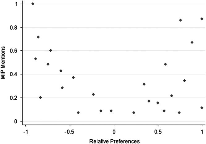
Figure 1 plots the hypothetical relationship between policy-based MIPs (on the y-axis) and relative preferences (on the x-axis). The depiction here is at the aggregate level, though a similar pattern applies at the individual level. The MIP scale between 0 and 1.0 indicates the fraction of respondents that mentions an issue, and the relative preferences scale between −1.0 and 1.0 indicates the net support for “less” or “more” policy. In the figure we can see a V-shaped pattern, owing to the fact that policy concerns undergird MIP responses. (Technically, we might expect a parabolic pattern instead.) People do not have problems in domains in which they are happy with the policy status quo—when they do not want more or less policy than is currently in place. They do have problems where they think the government should do more or less, that is, moving to the right or left of center along the x-axis.
Policy-based MIP and relative preferences.

There is a lot of variation in the pattern shown in the figure. This is not “noise;” it reflects the fact that not all of the domains to the left and right are the most important to many people. That MIP requires a forced choice—naming the single “most” important problem—is one factor. That importance is not perfectly correlated with preferences for policy change is another. Indeed, it may be that certain areas that have modest problems are more important to people than those with more severe problems.Footnote 8 What is important in Figure 1 is that where MIP responses strictly reflect policy concerns, they are not good substitutes for relative preferences. Consider that the Pearson’s correlation for the hypothetical data points in Figure 1 is trivial −0.16 (p=0.45). This implies that there is potentially no relationship whatsoever between measured MIP and R in practice.
Now let us consider cases in which MIP responses do not reflect policy concerns but register evaluations of conditions or outcomes instead. This conceptualization seems to better fit the empirical evidence (for example, Hibbs Reference Hibbs1979; Hudson Reference Hudson1994; Soroka Reference Soroka2002; Wlezien Reference Wlezien2005; Jennings and Wlezien Reference Jennings and Wlezien2011). Here people simply assess whether there is a problem with current conditions in different domains, and then choose the most important of these. Even if this is how people evaluate problems, MIP responses may still relate to policy preferences if they want the government to do something about problems. Specifically, we expect a positive relationship between relative preferences and MIP responses because, when focusing only on conditions, problems are defined asymmetrically: if there is a problem, conditions are worse than people would like. It is hard to imagine that people would have a problem if things are better than they want (that they would conclude that national security is too strong, there is too little crime, the environment is too clean or education is too good). In effect, focusing on conditions tends to increase the valence status of issues where voters are in broad agreement about the desirability of outcomes. To the extent that people want the government to do something about problems, we would expect a positive relationship between relative preferences and assessments of problems based on conditions. Of course, there will be a good deal of variation because importance varies across issues, and each individual has only one MIP, by definition.
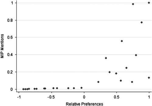
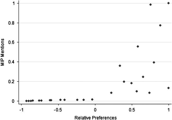
Figure 2 depicts the hypothetical relationship between outcome-based MIP and relative preferences. As discussed, the figure shows a positive relationship between the two. It reveals growing dispersion as R increases, owing to the variation in importance and the constrained choice of only the “most” important problem. The point is that people will want more policy in some domains that are most important problems and in others that are not. (In domains in which R is low, and people want less government, outcomes presumably are not problems.) Although it is not perfect, there is still a relationship between measured R and MIP. In the figure, the Pearson’s correlation between the hypothetical data points is 0.69 (p<0.01). Recall that this relationship is based on made-up numbers. In reality the relationship may be stronger than Figure 2 suggests. It also may be weaker. It may vary across policy domains. One possibility is that people do not want the government to do anything (or much) about the problems they identify. If this is so, we might expect very little connection between MIP and R. The problem is that we do not know how respondents formulate their MIP responses. We also do not know how much correspondence there is between those responses and relative preferences. That needs to be settled empirically.
Outcome-based MIP and relative preferences.
The Correspondence Between Public Preferences and Most Important Problems
Survey organizations have been asking about the MIP for many years. Gallup first asked the question in the US in 1935 and in the UK in 1947, specifically, “What is the most important problem facing the country today?” In the UK the wording was later changed to “Which would you say is the most urgent problem facing the country at the present time?”Footnote 9 Our analysis compares aggregate responses to these questions to relative preferences for spending over time in the two countries.Footnote 10 We examine spending preferences because this is the only subject that survey organizations have asked the public about on a regular basis, as noted above. Specifically, survey organizations have asked: Do you think the government is spending too much, too little or the right amount on (health)? The question has been asked for only a limited period of time: in the US, annually since 1972 and then in every other year since 2004; in the UK, first in 1961, and in most years between 1975 and 1995 (in 16 out of 21 years, with occasional gaps). These two countries afford us the longest possible time period over which we can observe differences or similarities between the measures.
Respondents have consistently been asked about spending preferences in a limited set of categories, which differs across countries: in the US, cities, crime, defense, education, the environment, foreign aid, health, space, parks, roads and welfare; in the UK, defense, education, health, pensions and roads. To characterize aggregate public preferences in each domain in each year (and country), we rely on “percentage difference” measures. There are calculated by taking the percentage that says the government is spending “too little” and subtracting the percentage saying “too much.” The measure is virtually indistinguishable over time from the mean preference, but it provides a much more intuitive empirical referent. In the analysis that follows, we refer to the measure as “net support” for spending.
In order to compare spending preferences and MIP responses, it is necessary to aggregate the latter into common categories. We were able to do this using MIP data from the Policy Agendas Project (www.policyagendas.org) and the UK Policy Agendas Project (www.policyagendas.org.uk), matching the preference data with the corresponding policy topics—this includes categories for defense, education, health, the environment, foreign aid, transport, crime and social welfare.Footnote 11 (The numerical topic code for the Policy Agendas Project is reported in the left-hand column of Table 1, below.) The MIP data is simply the percentage of MIP mentions referring to a given topic, taking a value between 0 and 100 percent.
Correlation of MIP and Preferences for Spending (GSS)

Note: N in parentheses, *p≤0.05; **p≤0.01.
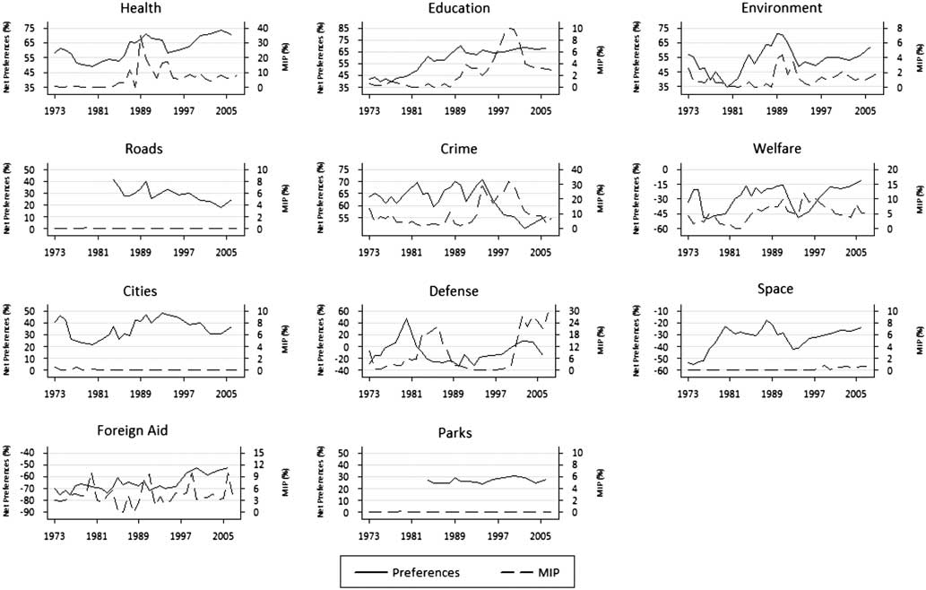
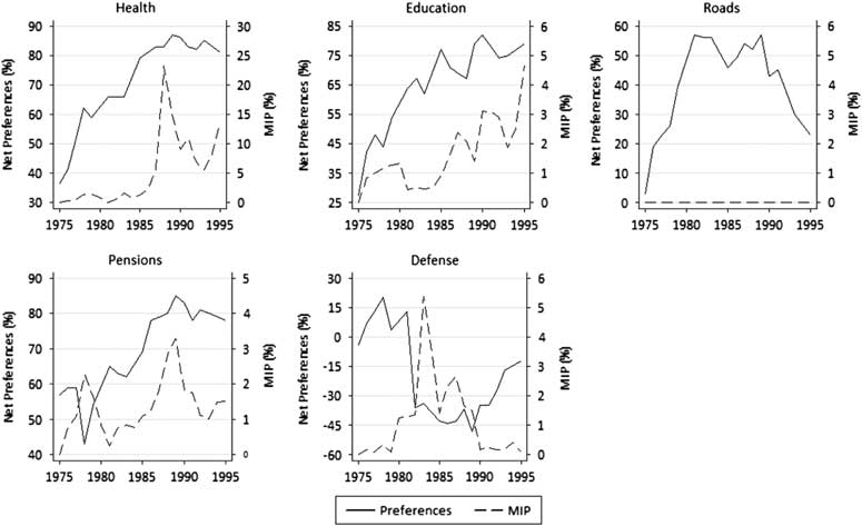
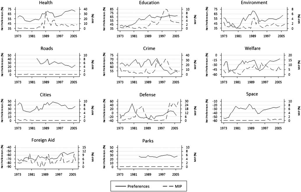
Figures 3 and 4 plot public spending preferences and MIP responses in each of the policy areas in the US and UK. The figures are revealing. To begin with, we can see that the measures often differ at particular points in time. This is perfectly understandable, given the differences in the scales of the two variables, and it tells us little about their correspondence. What interests us is the relationship over time, which the figures suggest varies across issues and countries. In Figure 3, US spending preferences and MIP responses tend to move together in some domains—health and environment—but not in others. Figure 4 appears to reveal more correspondence in the UK, at least in the three domestic policy areas (health, education and pensions). It is notable that there is no correspondence whatsoever between preferences and MIP responses for a number of categories that are extremely low in salience—that is, when the mean of MIP responses tends toward zero: roads, space and parks in the US and roads in the UK.Footnote 12
MIP and preferences, US, 1973–2006.
MIP and preferences, UK, 1975–95.
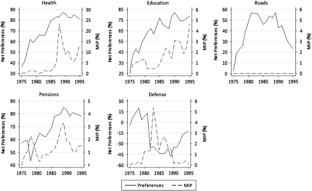
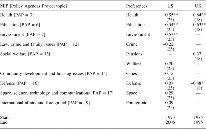
Table 1 provides a statistical analysis. It contains Pearson’s correlations between preferences and MIP responses for each of the categories, with results for the US and UK shown in separate columns. In the table we can see that MIP responses and relative preferences are not closely related over time. The correlations are positive in 10 of the 13 cases, but significantly greater than zero in only five: for health and education in both the US and UK and for the environment in the US.Footnote 13 Even in these five cases, the correlations average below 0.60. In one case, defense in the UK, the correlation is negative and statistically significant. That is, when defense is considered to be a problem, the public supports less spending, not more. For the full set of 13 cases, the mean correlation is a meager 0.24. The relationship is slightly stronger in the UK, as we see positive, significant correlations in two of the four cases there and a larger mean correlation—0.29 compared with 0.22 in the US.
Before drawing any conclusions about cross-national differences, it is important to note that the difference in mean correlations is small and not statistically significant. Even to the extent that there are differences between the US and UK, these may reflect differences in the number and types of policy domains for which data on relative preferences is available—in the UK, we have data for a handful of comparatively salient domains. In any event, we are not primarily concerned with differences across countries, and what is clear from our analysis in both countries is that MIP and preferences tap different things. Less than one-tenth of the variance is common to the two measures on average; that is, 90 percent is unique. This is not very different in policy domains in which the two measures are most highly correlated, as here about one-third of the variance is common. Although the estimates of uniqueness are inflated by measurement error, they still reveal substantial differences between MIP and spending preferences.
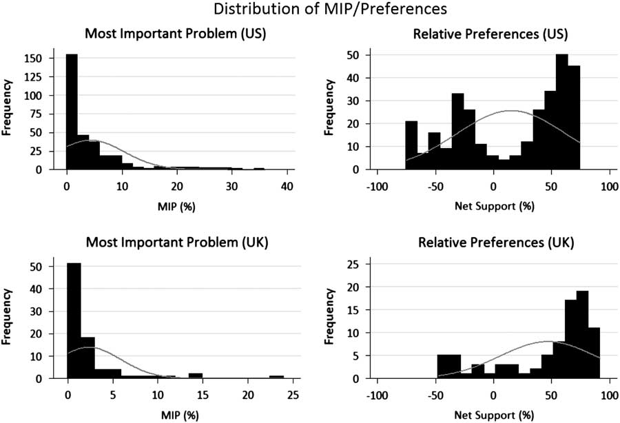
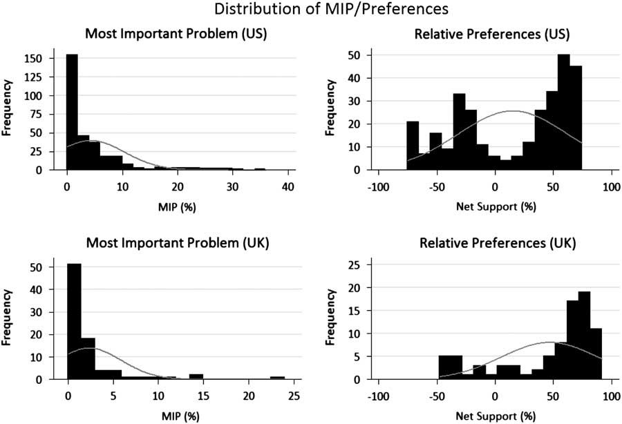
The statistical properties of the MIP and preference series also differ substantially. Some domains (for example, the economy and defense) are consistently more important than others, and so variation in their problem status has a sizeable effect on MIP responses, whereas in other domains problem status does not matter (Wlezien Reference Wlezien2005). This means that some issues have restricted variance.Footnote 14 This is more likely to generate distributions of MIP that are skewed and non-normal (Jones and Baumgartner Reference Jones and Baumgartner2005; also see Jennings and John Reference Jennings and John2009). This is confirmed in Figure 5, in which a large number of MIP responses are equal to or close to zero, and the distribution of net support for spending is more evenly spread. The distributions of MIP responses exhibit positive kurtosis, whereas relative preferences are bimodal.Footnote 15 Further, the MIP distributions are more skewed, due to clustering of the peak of the distribution close to zero. Practically, the restricted variance of MIP compared to relative preferences may further reduce the degree of correspondence between these measures for some issues (Achen Reference Achen1990).
Distributions of MIP responses and relative preferences in the US and UK.
The results thus demonstrate that MIP responses are not a good substitute for relative preferences in most spending domains. Although they may indicate preferences in some areas, this is the exception, not the rule. Even here, they are partial indicators. This is precisely as we hypothesized above, where MIP responses reflect public assessments of conditions, not policy per se. (Of course, it may be that they reflect both policy and conditions.)
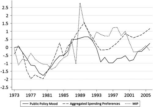
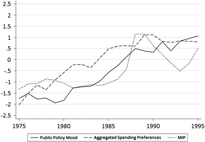
Although MIP responses may not work well in specific spending domains, they may function better for related policy domains taken together. For instance, MIP responses for the aggregation of policy areas may serve to indicate relative preferences for general government policy.Footnote 16 We can test this proposition in two ways, focusing particularly on “social” domains. First, it is possible to assess the degree of correspondence between MIP responses on social issues (the sum of MIP responses for the civil rights, health, welfare, education, environment and housing categories) and aggregated spending preferences in the same domains (the average of net support for spending for health, environment, education, welfare and cities in the US and for health, pensions and education in the UK). Second, it is possible to substitute Stimson’s public policy mood, that is, citizens’ relative preference for either more liberal or more conservative government policy in general (Stimson Reference Stimson1991; Erikson, MacKuen and Stimson Reference Erikson, MacKuen and Stimson2002; Bartle, Dellepiane-Avellaneda and Stimson Reference Bartle, Dellepiane-Avellaneda and Stimson2011). We know that these alternative measures of relative preferences – regarding spending and policy in general – are closely correlated (Wlezien Reference Wlezien1995). The two series are plotted alongside MIP responses on social issues in Figures 6 and 7 on a standardized scale. There we can see that the three measures exhibit a degree of common movement over time.
Domestic MIP and aggregate public policy preferences, US, 1973–2006.

Domestic MIP and aggregate public policy preferences, UK, 1975–95.
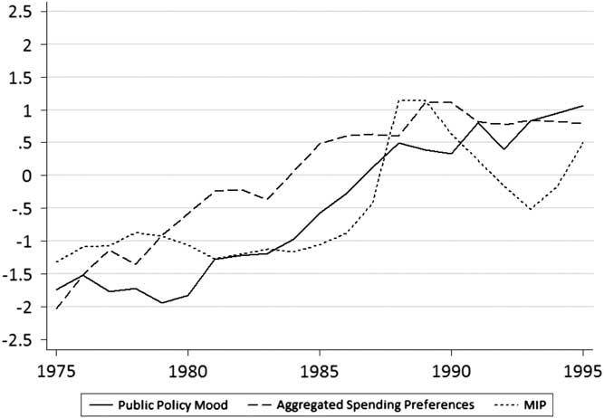
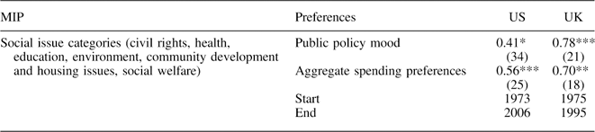
Table 2 presents an analysis of the two measures of aggregate preferences and MIP totals for social policy domains. Understandably, the results largely summarize what we saw in Table 1: modest relationships between the variables that are stronger in the UK. The correlations with social spending preferences reported in Table 2 are about twice as large as the average correlations across spending domains from Table 1. This partly reflects the fact that the analysis in Table 2 combines policy areas that show the closest correspondence. Consider that the average correlations for the “social” domains in Table 1—0.34 in the US and 0.55 in the UK—are not that much lower than in Table 2, where they are combined. MIPs for related (social) domains seemingly do not work significantly better when preferences for spending are taken together or when public preferences for government policy are measured on a general left-right dimension.Footnote 17 Our findings in Tables 1 and 2 may be a best case for the relationship between MIP and preferences. Consider that when we estimate correlations of the first differences of MIP responses and relative preferences for specific domains, we find no significant relationships for either the US or the UK.Footnote 18 The same is true for the correlation of MIPs and preferences in the combined social domains. The relationship between MIPs and preferences is at best modest and typically weak.
Correlation between Aggregations of MIP (Social Issues) and Preferences

Note: N in parentheses, *p≤0.05; **p≤0.01; ***p≤0.001, with gaps for preference series.
The Consequences of Measurement
We have seen that MIP responses are generally poor substitutes for the public’s relative spending preferences, but that the performance varies across domains. Now we want to see what difference the measures make. This is interesting unto itself but also important, as it allows us to assess whether (and how) the observed differences in the measures really do matter, and how this varies across domains. For this analysis, we focus on policy responsiveness in different domains. If there is responsiveness, the change in policy (ΔPt) will be a function of relative preferences (R), which reflects support for policy change. Other things also matter for policy, of course, including the partisan control of government (G). Note that both R and G are lagged to reflect preferences and party control when budgetary policy, the focus of our empirical analysis, is made.Footnote 19 For any particular domain, then, the equation is:
 $$\Delta {\rm P}_{t} ={\rm \rrho }{\plus}{\rm \rgamma }_{{\rm 1}} {\rm R}_{{t{\minus}{\rm 1}}} {\plus}{\rm \rgamma }_{{\rm 2}} {\rm G}_{{t{\minus}{\rm 1}}} {\plus}{\rm \rmu }_{t} ,$$
where ρ and μt represent the intercept and the error term, respectively. The equation captures both responsiveness and indirect representation. The latter—representation through election results and subsequent government partisanship—is captured by γ2, and the former—adjustments to policy reflecting shifts in preferences—is captured by γ1. Other variables can be added to the model, of course.
The coefficient γ1 is most critical for our purposes. It captures policy responsiveness, the kind of dynamic representation that we expect to differing degrees across policy domains. A positive coefficient need not mean that politicians literally respond to changing public preferences, of course, as it may be that they and the public both respond to something else, for example, changes in the need for more spending. All we can say for sure is that γ1 captures policy responsiveness in a statistical sense—the extent to which policy change is systematically related to public preferences, other things being equal.Footnote 20 This is of (obvious) importance, as we want to know whether public policy follows public preferences.
The dependent variable in our analysis is the change in government spending in each particular domain. In the US, we rely on measures from the Historical Tables published by the Office of Management and Budget, with temporally consistent functions back to 1972, the first year for which have preference data. In the UK, there are problems with the reliability of government data, and so we rely on Soroka, Wlezien and McLean’s (Reference Soroka, Wlezien and McLean2006) re-recalculations of spending back to 1980. When combined with two years of earlier data recalculated by HM Treasury for Public Expenditure Statistical Analysis, we have functionally consistent data from 1978 to 1995, the last year for which preference data are available. We adjust all of the measures for inflation.Footnote 21
As noted above, the models include measures of the party composition of government. In the US, there are measures for the president and Congress. The former variable takes the value 1 under Democratic presidents and 0 under Republican presidents, and the latter variable represents the average percentage of Democrats in the House and Senate. In the UK, party control of government is coded 1 under Conservative governments and 0 under Labour governments. As for net support, these political variables are measured during year t−1. Models in selected UK domains (education and health) also include the unemployment rate.Footnote 22
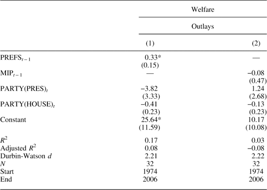
Now, we are interested in seeing what difference it makes to use MIP responses in place of relative preferences. To make this assessment, we first estimate Equation 2 for each spending domain using our measures of net support and then estimate the same equation using MIP responses in place of net support. To begin with, we present these two estimated equations for the US welfare spending domain. The results are shown in Table 3.
Welfare Spending Representation, US

Note: *p≤0.05.
In the first column of Table 3 we see that changes in welfare spending do follow public preferences for spending in that domain over time. As indicated by the positive, significant coefficient (0.33) for net support, when the public preference for more spending is high, politicians tend to provide more spending. A one-point increase in support for more spending in year t−1 leads to a $0.33 billion increase in year t. This is evidence of policy responsiveness; that is, spending changes in response to preferences independently of party control of government, which itself may reflect preferences. (However, neither party control of the presidency nor Congress reliably influences welfare spending.)
Using MIP in place of preferences produces very different results. The coefficient for welfare MIP (−0.08) on spending is negative, though not statistically significant. Model performance also is inferior, with the R 2 equal to just 0.03 compared to 0.17 using the measure of spending preferences. The evidence is thus clear: the measures matter, and in fundamental ways. Welfare MIP is not at all a good substitute for actual spending preferences. Of course, this is just one domain in one country.
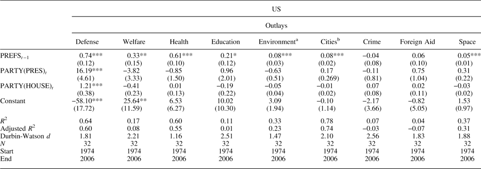
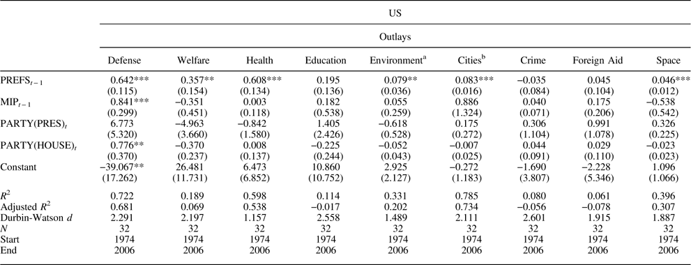
Let us next compare the pattern of dynamic representation across all domains, in both the US and the UK. First, in Table 4 we present the results from estimating the equation in each US spending domain, using measures of public preferences. Here there is unmistakable evidence of representation of preferences, with positive and significant coefficients in seven out of the nine domains. An increase in support for spending in year t−1 leads to an increase in spending in year t, just as for welfare spending. The size of the effect varies across domains, however. For example, a one-point increase in net support for defense spending leads to a $0.74 billion increase, whereas a one-point increase in net support for the environment leads to a $0.08 billion increase. Only for crime and foreign aid do we fail to detect representation using spending preferences.
Spending Representation, US (Preferences)

Note: aIncludes dummy for FY1977; bIncludes dummy for FY1977 and FY1978; *p≤0.1; **p≤0.05; ***p≤0.01.
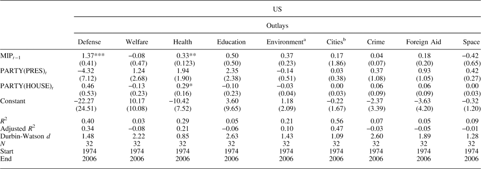
The results using MIP responses in the US, summarized in Table 5, show much less evidence of representation. Positive and significant coefficients are observed for just two issues: defense and health. When MIP is used as substitute for preferences, an increase in public concern about an issue is typically not translated into a change in spending. Further, the models using preferences tend to explain far more variation than those using MIP, that is, the R 2 is greater in all but one case, and the average R 2 is equal to 0.35 compared to 0.19. This is true even in the defense and health domains, in which MIP responses have positive effects on spending. Thus, from the US case it is clear that MIP responses are not good substitutes for spending preferences, which has substantively important implications for inferences about dynamic representation: when MIP is used, the degree of correspondence between public opinion and policy is far weaker and spotty.
Spending Representation, US (MIP)

Note: aIncludes dummy for FY1977; bIncludes dummy for FY1977 and FY1978; *p≤0.1; **p≤0.05; ***p≤0.01
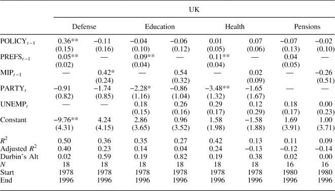
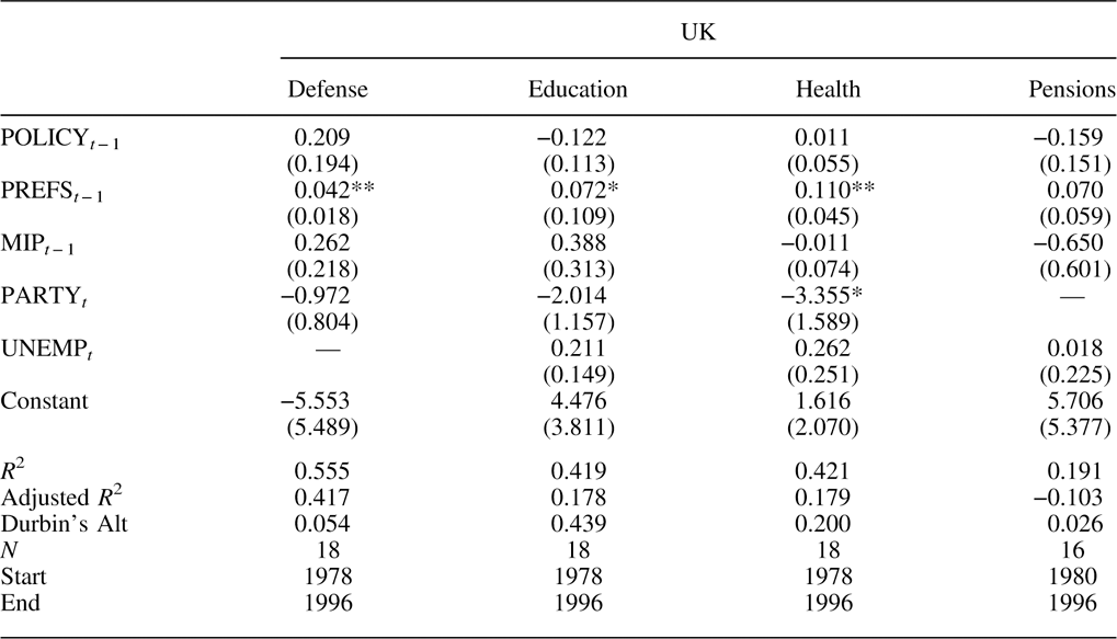
Now let us turn to the UK. Table 6 shows the results of estimating the equation using measures of preferences and MIP responses in the UK.Footnote 23 Using spending preferences, there is substantial evidence of representation, with positive and significant coefficients in three out of the four domains—defense, health and education. For instance, a one-point increase in net support in year t−1 leads to a £0.36 billion increase in defense spending in the following year. (Adjusting for the exchange rate during the period, the effect is virtually identical to that in the US.) In contrast, the effect of MIP on spending is positive and significant in just one case—defense. The coefficient is negative for education and pensions, although not statistically significant. Again, model performance is better for spending preferences than for MIP responses: the R 2 is greater in all cases, and the average R 2 is equal to 0.35 compared to 0.21. In the UK, MIP responses are not good substitutes for spending preferences, and using them significantly impacts the inferences we make.
Spending Representation, UK (Preferences and MIP)

Note: *p≤0.1; **p≤0.05.
Together, the results for the US and the UK point to the same pattern: there is far greater evidence of representation when measured preferences are used instead of MIP responses. Moreover, when MIP and preferences are included in the same model, MIP has a positive and significant effect in just one case (defense in the US), whereas preferences are statistically significant in nine out of 13 cases. For details, see Appendix Tables A1 and A2. Keep in mind that these findings do not include models for spending in domains in which MIP responses are virtually zero over the time period—roads and parks in the US and roads in the UK. If anything, therefore, our analyses exaggerate the degree to which MIP responses can serve as effective substitutes for preferences in the study of representation.
Conclusion
MIP responses clearly are not public policy preferences. Based on our analysis of the US and UK, they are also poor substitutes. They are more closely related in some policy domains than in others, but not very well even there. We find that using MIP in place of preferences also matters a lot for models of dynamic representation. The results differ substantially: preferences have a positive and statistically significant effect on government spending in ten out of 13 domains, whereas MIP responses have an effect in just three out of 13. This leads us to draw quite different conclusions about the functioning of representative democracies. Specifically, the use of MIP introduces Type II error, leading us to substantially understate the level and extent of opinion representation in policy. While the US and UK political systems may not be “most different,” they are quite different—a federal-presidential system versus a unitary-parliamentary system. The common patterns thus suggest general patterns, though a definitive conclusion awaits research in other countries.
MIP responses might sometimes be usable as a substitute for preferences in certain domains, but this is the exception rather than the rule. The relationship between MIP and relative preferences depends on what people think about when identifying their MIP. When focusing only on conditions, problems are defined asymmetrically, where conditions are worse than people would like (that is, people rarely desire “more crime,” “more unemployment” and so on). As discussed above, there may be a degree of correspondence between MIP and preferences in such cases, as MIP mentions will tend to increase as conditions worsen and people want the government to do something about it, i.e., enact more policy. It is notable that the domain in which the effect of MIP is found to be significant in both countries, defense, is one of the archetypal valence issues (Stokes Reference Stokes1963).Footnote 24 Recall that, even in these cases, we do not expect the relationship to be perfect, for at least two reasons: (1) people may not want more policy in response to bad conditions (and actually may want less) and (2) people may want more policy even if conditions are good.
Even though MIP responses are poor indicators of public spending preferences, this does not mean that they contain little meaningful information about public opinion on policy. Nor does it suggest that MIP has no broader utility for the study of policy. As we have discussed, MIP responses tap public attention to issues both at particular points in time and over time. That is, they reveal a lot about the areas in which the public wants the government to take action. This is important because attention is crucial to policy making (for example, Jones and Baumgartner Reference Jones and Baumgartner2005), and MIP has clear utility in tracing the issues that the public is attending to at any moment in time. Specifically, MIP provides a measure of priorities, indicating which issue is most important for both individuals and the public in the aggregate. As such, there is reason to suppose that MIP will account for much of the variation in policy activism across domains at particular points in time—that is, where MIP is high (low) we expect much (little) policy activity. MIP responses are not perfect indicators of attention, however, as the total number of mentions remains (largely) fixed over time, due to the survey question requiring respondents to choose a single important problem even where they have more than one.Footnote 25
The relative ranking of issues as problems at the aggregate level may also work well as a measure of priorities. Although MIP responses tend to reflect variation in problem status rather than the importance of issues to the public, they do appear to indicate the general importance of issues when aggregated over long stretches of time (see, for example, Soroka and Wlezien Reference Soroka and Wlezien2010). This evidently averages out the variation in problem status, making the underlying importance of the domains (more) visible. MIP responses might also reveal useful information about the importance of issues across individuals at particular points in time (Bartle and Laycock Reference Bartle and Laycock2012). They could provide information about differences in the importance of issues across contexts as well. MIP is not equivalent to preferences, however, and a good measure of one does not work well as a measure of the other. Most importantly, using MIP responses in the study of public opinion and policy has substantive consequences for our understanding of how representative democracy works.
Supplementary material
To view supplementary material for this article, please visit http://dx.doi.org/10.1017/S2049847015000035
Appendix
Spending Representation (Using Both MIP and Preferences), US

Spending Representation (Using Both MIP and Preferences), UK