2.1. Frequency-based BMS

In the classical BMS, both the a priori and a posteriori classification are fully determined by the frequency while ignoring the severity. We present a random effect model for this BMS, calling it “the frequency model” under the general frame work of generalized linear models (GLMs) [Reference Nelder and Wedderburn16]. For a given policyholder, the frequency model consists of several components, described as follows.

The frequency, $N_{t}$, of a given policyholder in the $t$th policy year is specified using a count regression model conditioning on $\boldsymbol {X}^{[1]}=\boldsymbol {x}_\kappa ^{[1]}$ and $\Theta ^{[1]}=\theta ^{[1]}$, that is,

$$N_{t}\,\vert\,(\boldsymbol{x}_\kappa^{[1]},\theta^{[1]}) \overset{\textrm{i.i.d.}}{\sim} F_1({\cdot}; \lambda_\kappa^{[1]}\theta^{[1]}, \psi^{[1]} ),$$

for some discrete distribution $F_1$ with the mean parameter $\lambda _\kappa ^{[1]}\theta ^{[1]}$ and the other parameter $\psi ^{[1]}$. Following the convention, the a priori rate is modeled as $\lambda _\kappa ^{[1]}= (\eta ^{[1]})^{-1}(\boldsymbol {x}_\kappa ^{[1]}\boldsymbol {\beta }^{[1]})$, where $\boldsymbol {\beta }^{[1]}$ is the regression coefficient vector to be estimated from the data. Hence, having information on $\boldsymbol {x}_\kappa ^{[1]}$ is equivalent to knowing $\lambda _\kappa ^{[1]}$, provided that the model has been fully specified. For the brevity of exposition, we will use $\lambda _\kappa ^{[1]}$ instead of $\boldsymbol {x}_\kappa ^{[1]}$ when the a priori characteristics $\boldsymbol {x}_\kappa ^{[1]}$ appear as a conditional quantity; for example, ${\mathbb {E}}[{N_{T+1}\,\vert \, \lambda _\kappa ^{[1]}, \theta ^{[1]}}]$ will be used instead of ${\mathbb {E}}[{N_{T+1}\,\vert \, \boldsymbol {x}_\kappa ^{[1]}, \theta ^{[1]}}]$. Note that $\lambda _\kappa ^{[1]}$ and $\theta ^{[1]}$ vary over policyholders, whereas $\psi ^{[1]}$ remains constant, common for all policyholders. As such, we will suppress this common parameter for quantities that do not vary over individual policyholders. In a special case where $F_1 \in$ EDF, $\psi ^{[1]}$ becomes the common dispersion parameter.

By definition, the observations $N_t$ are conditionally independent given the a priori risk characteristics $\boldsymbol {x}_\kappa ^{[1]}$ and residual (or random) effect $\theta ^{[1]}$, but are dependent unconditionally. We assume that $\Theta ^{[1]}$ is distributed as

$$\Theta^{[1]}\overset{\textrm{i.i.d.}}{\sim} G_1,$$

where $G_1$ is a distribution function. Individual policyholders have different realizations of $\Theta ^{[1]}$, which capture the residual heterogeneity; it is assumed that ${\mathbb {E}}[{\Theta ^{[1]}}] =1$ for convenience, following the convention.

The ideal premium for the next year in this frequency model is the hypothetical mean, also known as individual premium in the credibility literature, written as

$${\mathbb{E}}[{N_{T+1}\,\vert\, \lambda_\kappa^{[1]}, \theta^{[1]}}].$$

This, however, can be numerically obtained only when $(\Lambda ^{[1]}, \Theta ^{[1]})$ are known. While $\Lambda ^{[1]}$ is known at the outset of the contract and remains fixed over time, the value of $\Theta ^{[1]}$ is never known, as it is a random variable. The solution is then to revise the distribution parameters of $\Theta ^{[1]}$ based on the past claim frequency history $\mathcal {F}_{T}^\textrm {[freq]}$ and compute the predictive mean ${\mathbb {E}}[{N_{T+1}\,\vert \, \lambda _\kappa ^{[1]}, \mathcal {F}_{T}^\textrm {[freq]} }]$. This is called the Bayesian premium.

Although the Bayesian premium is deemed to be the best premium possible, most ratemaking systems in the auto insurance industry maintain a BMS, which can be considered a discrete approximation of the Bayesian premium, as explained below. The classical BMS constitutes three elements: the BMS levels, transition rule, and relativities. Without loss of generality, let us assume that the insurer has $z+1$ BM levels varying from $0$ to $z$, with $-1/+h$ system as a transition rule. Thus, in this system, a claim-free year is rewarded by moving one BM level downward, while each reported claim, regardless of the claim size, is penalized by climbing $h$ levels per claim at the end of the period. Theoretically, the choice of the number of BM levels and the transition rule are arbitrary, though insurers may have constraints subject to local regulations in practice. The transition rule affects how the drivers are populated over $z+1$ different BM levels, which, in turn, determines the optimal premium of a driver in each level for the following year.

The last element of the classical BMS is the relativity. In the classical frequency-driven BMS, the relativity associated with BM level $\ell$, denoted by ${r}^\textrm {[freq]}(\ell )$, is used to predict the frequency in the next year through the multiplicative form

(1) \begin{equation} \lambda_\kappa^{[1]}r^\textrm{[freq]}(\ell), \quad \ell=0,\ldots,z, \end{equation}

where the a priori rate $\lambda _{\kappa }^{[1]}= (\eta ^{[1]})^{-1}(\boldsymbol {x}_{\kappa }^{[1]}\boldsymbol {\beta }^{[1]})$ reflects the risk class to which the policyholder belongs. Expression (1) is obtained from the following minimization by Tan et al. [Reference Tan, Li, Li and Balasooriya22]:

$$(\tilde{r}^\textrm{[freq]}(0), \ldots, \tilde{r}^\textrm{[freq]}(z))={\arg\, \min}_{({r}(0), \ldots, {r}(z))\in \mathbb{R}^{{z+1}}} {\mathbb{E}}\left[{( \mathbb{E}[{N_{T+1}\,\vert\, \Lambda^{[1]}, \Theta^{[1]}}]-\Lambda^{[1]}{r}(L))^{2}}\right],$$

where $L$ denotes the BM level occupied by a randomly selected policyholder in the steady stateFootnote ¹ under $-1/+h$ system.

2.2. BMS based on both frequency and severity

Though widely used in practice, the frequency-based BMS completely ignores the claim severity information. A more statistically solid approach would be based on the aggregate severity, or the total loss of the collective risk model, which reflects both claim frequency and severity. In traditional collective risk models, the frequency and severity are assumed independent. Although a series of recent studies shows that this unwarranted assumption can be relaxed in the collective risk model, and, thus, further in the Bayesian premium and BMS. In fact, the dependence between the frequency and severity in auto insurance is shown to be statistically significant in recent empirical studies such as Frees et al. [Reference Frees, Lee and Yang8] and Garrido et al. [Reference Garrido, Genest and Schulz9].

While various dependent collective risk models exist as mentioned in the “Introduction” section, including the two-step frequency–severity model and the copula-based model, we find that the bivariate random effect model is most convenient for the development of a better BMS because of its conditioning structure in the model specification. In this section, we focus on the model by Oh et al. [Reference Oh, Shi and Ahn17], as it offers the most comprehensive bivariate random effect model: It contains other existing bivariate random effect models in the literature—Pinquet [Reference Pinquet20], Boudreault et al. [Reference Boudreault, Cossette, Landriault and Marceau2], Hernández-Bastida et al. [Reference Hernández-Bastida, Fernández-Sánchez and Gómez-Déniz11], Baumgartner et al. [Reference Baumgartner, Gruber and Czado1], Lu [Reference Lu14], and Cheung et al. [Reference Cheung, Ni, Oh and Woo3]—as special cases.

Paralleling the frequency model in Section 2.1, the dependent collective risk model of Oh et al. [Reference Oh, Shi and Ahn17] is specified as follows. We call this “the frequency–severity model,” as it requires both frequency and severity models. For the given a priori rate $(\Lambda ^{[1]}, \Lambda ^{[2]})=(\lambda _\kappa ^{[1]}, \lambda _\kappa ^{[2]})$ and residual effect $(\Theta ^{[1]}, \Theta ^{[2]})=(\theta ^{[1]}, \theta ^{[2]})$, the observations

$$N_{t} \quad \text{and}\quad Y_{t,j}\quad\text{for}\;\; t,j\in\mathbb{N}$$

are independent. In the frequency–severity model, the distributional assumption for $N_t$ is identical to the frequency model in Section 2.1. The individual severity $Y_{t,j}$ is specified using a regression model conditioning on the a priori risk characteristics $\boldsymbol {X}^{[2]}=\boldsymbol {x}_\kappa ^{[2]}$, or equivalently $\Lambda ^{[2]}=\lambda _\kappa ^{[2]}$ as previously mentioned, and the residual effect $\Theta ^{[2]}$, such that

$$Y_{t,j}\,\vert \,( \lambda_\kappa^{[2]}, \theta^{[2]}) \overset{\textrm{i.i.d.}}{\sim} \textrm{EDF}( \lambda_\kappa^{[2]}\theta^{[2]}, \psi^{[2]}),$$

where the EDF has mean parameter $\lambda _\kappa ^{[2]}\theta ^{[2]}$ with $\lambda _\kappa ^{[2]}=(\eta ^{[2]})^{-1}(\boldsymbol {x}_\kappa ^{[2]} \boldsymbol {\beta }^{[2]})$ and dispersion parameter $\psi ^{[2]}$. Finally, the residual effect characteristic $(\Theta ^{[1]},\Theta ^{[2]})$, which is assumed to be independent of the a priori rate $(\Lambda ^{[1]}, \Lambda ^{[2]})$, has a joint distribution $H$. That is,

(2) \begin{equation} (\Theta^{[1]}, \Theta^{[2]} )\overset{\textrm{i.i.d.}}{\sim} H=C(G_1, G_2 ), \end{equation}

where $G_1$ and $G_2$ denote the marginal distribution functions for $\Theta ^{[1]}$ and $\Theta ^{[2]}$, respectively, and $C$ is a bivariate copula that defines the dependence structure in $H$. We use $g_1$, $g_2$, and $h$ to denote the density functions of $G_1$, $G_2$, and $H$, respectively. As before, it is further assumed

$${\mathbb{E}}[{\Theta^{[1]}}] = {\mathbb{E}}[{\Theta^{[2]}}] = 1$$

for convenience.

There are several conditional independence relations under this frequency–severity model specification. For example, given $(\lambda _\kappa ^{[1]}, \lambda _\kappa ^{[2]})$, and $(\theta ^{[1]}, \theta ^{[2]})$, the claim history $(N_{t}, \boldsymbol {Y}_{t})$ of a given policyholder is independent across time, and independence between frequency and individual severities and independence among individual severities are further implied. However, marginally or unconditionally, various dependence relations are observed:

• • Dependence among frequencies induced by residual effect $\Theta ^{[1]}$;

• • Dependence among severities induced by residual effect $\Theta ^{[2]}$;

• • Dependence between frequency and severity induced by residual effects $(\Theta ^{[1]},\Theta ^{[2]}$) via the copula $C$.

Recalling that the individual severity $Y_{t,j}$ is assumed EDF distributed, we note that the conditional average severity is again EDF distributed. That is,

$$M_{t}\,\vert\, (\lambda_\kappa^{[1]}, \lambda_\kappa^{[2]},\theta^{[1]},\theta^{[2]}, N_{t}) \overset{\textrm{i.i.d.}}{\sim} \textrm{ED}( \lambda_\kappa^{[2]}\theta^{[2]}, \, \psi^{[2]}/N_{t}), \quad N_{t}>0,$$

and

$${\mathbb{P}}({M_{t}=0\,\vert\, \lambda_\kappa^{[2]},\theta^{[2]}, N_{t} })=1, \quad \text{if }N_{t}=0,$$

where the mean parameter of the EDF, $\lambda _\kappa ^{[2]}\theta ^{[2]}$, is modeled through $\lambda _\kappa ^{[2]}=(\eta ^{[2]})^{-1}(\boldsymbol {x}_\kappa ^{[2]} \boldsymbol {\beta }^{[2]})$. Thus, the distribution of $M_t$ is the same as that of $Y_{t,j}$, except for the dispersion parameter. This allows us to efficiently model the aggregate severity $S_t$ as a product form $N_t M_t$, whose mean serves as the premium under the frequency–severity model. There are two noteworthy sub-modes of the frequency–severity model. First, it reduces to the frequency model in Section 2.1 by removing the severity part. Second, if the copula $C$ embedded in $H$ is an independent copula, then the frequency and severity can be independently modeled, leading to the standard collective risk model.

We found that the optimal frequency-premium takes a form of $\lambda _\kappa ^{[1]}\tilde {r}^\textrm {[freq]}(\ell )$ in the frequency model from (1). Now, suppose we predict the aggregate severity as the premium using the history of the frequency only. A simple, but widely, used approach in the literature [Reference Denuit, Maréchal, Pitrebois and Walhin5] is to multiply the average severity of all policyholders in the same risk class to the frequency such that the BMS premium is predicted with

(3) \begin{equation} \lambda_{\kappa}^{[1]}\tilde{r}^\textrm{[freq]}(\ell) \times \lambda_{\kappa}^{[2]}. \end{equation}

This multiplicative form is less than ideal in at least two aspects. First, by incorporating the average severity of the entire portfolio, it reflects the history of the frequency of a given policyholder, but completely ignores the past severity records of individual policyholders. Second, the multiplicative form can be justified only when the independence of the frequency and severity is warranted, which is not valid in general. In fact, the BMS premium (3) is motivated from the following Bayesian premium with the implied independence between frequency and severity:

(4) \begin{equation} {\mathbb{E}}[{S_{T+1}\,\vert\, \lambda_\kappa^{[1]}, \lambda_\kappa^{[2]}, \mathcal{F}_{T}^\textrm{[freq]} }] =\lambda_\kappa^{[1]}{\mathbb{E}}[{\Theta^{[1]}\,\vert\, \lambda_\kappa^{[1]}, \lambda_\kappa^{[2]}, \mathcal{F}_{T}^\textrm{[freq]} }] \times \lambda_\kappa^{[2]}. \end{equation}

From this, the relativity $\tilde {r}^\textrm {[freq]}(\ell )$ in (3) can be interpreted as the BMS version of the posterior estimation

$${\mathbb{E}}[{\Theta^{[1]}\,\vert\, \lambda_\kappa^{[1]}, \lambda_\kappa^{[2]}, \mathcal{F}_{T}^\textrm{[freq]} }]$$

in (4). Therefore, while convenient and simple, the BMS premium (3) may result in a considerable bias when dependence between frequency and severity is strong. To adjust such bias, Oh et al. [Reference Oh, Shi and Ahn17] suggested the following BMS premium from a policyholder at BM level $\ell$ in a $-1/+h$ system under the frequency–severity model:

(5) \begin{equation} \lambda_{\kappa}^{[1]}\lambda_{\kappa}^{[2]} \tilde{r}^\textrm{[dep]}(\ell), \quad \ell=0,\ldots,z, \end{equation}

where optimal relativity $\tilde {r}^\textrm {[dep]}(\ell )$ for $\ell =0,\ldots ,z$ is the solution of the optimization,

(6) \begin{align} & (\tilde{r}^\textrm{[dep]}(0), \ldots, \tilde{r}^\textrm{[dep]}(z))\nonumber\\ & \quad ={\arg \, \min}_{({r}(0), \ldots, {r}(z))\in \mathbb{R}^{{z+1}}} {\mathbb{E}}\left[{( \mathbb{E}[{S_{T+1}\,\vert\, \Lambda^{[1]}, \Lambda^{[2]}, \Theta^{[1]}, \Theta^{[2]} }]-\Lambda^{[1]}\Lambda^{[2]}{r}(L))^{2}}\right] \end{align}

which is an extended setting of that in Tan et al. [Reference Tan, Li, Li and Balasooriya22]. Here, $L$ denotes the BM level occupied by a randomly selected policyholder in the steady state under the $-1/+h$ system. We refer to Oh et al. [Reference Oh, Shi and Ahn17] for the detailed derivation of (6).

Similar to (3), the premium (5) can be viewed as the BMS version of the Bayesian premium from

(7) \begin{equation} {\mathbb{E}}[{S_{T+1}\,\vert\, \lambda_\kappa^{[1]}, \lambda_\kappa^{[2]}, \mathcal{F}_{T}^\textrm{[freq]} }] =\lambda_\kappa^{[1]}\lambda_\kappa^{[2]} {\mathbb{E}}[{\Theta^{[1]}\Theta^{[2]}\,\vert\, \lambda_\kappa^{[1]}, \lambda_\kappa^{[2]}, \mathcal{F}_{T}^\textrm{[freq]} }] \end{equation}

and, consequently, the relativity $\tilde {r}^\textrm {[dep]}(\ell )$ in (5) can be interpreted as the BMS version of the posterior estimation

(8) \begin{equation} {\mathbb{E}}[{\Theta^{[1]}\Theta^{[2]}\,\vert\, \lambda_\kappa^{[1]}, \lambda_\kappa^{[2]}, \mathcal{F}_{T}^\textrm{[freq]} }]. \end{equation}

Notably, the BMS premium of Oh et al. [Reference Oh, Shi and Ahn17] operates under the $-1/+h$ system, where the BM level transition is driven by the claim frequency only and is unable to penalize high severity claims. Also, as seen from (8), the severity history is not used inside the condition. In reality, the severity information is indirectly incorporated only through the dependence between $\Theta ^{[1]}$ and $\Theta ^{[2]}$. Thus, the BMS premium of Oh et al. [Reference Oh, Shi and Ahn17] approximates the Bayesian premium, but in a limited sense, because it incorporates the history of claim frequency and not severity. Later, we propose to improve the BMS premium prediction with a direct incorporation of the history of severity as well.

2.3. Motivation for transition rules driven by the severity history

As discussed in the previous subsection, the BMS premium of Oh et al. [Reference Oh, Shi and Ahn17] in (5) can be viewed as the BMS version of the Bayesian premium in (7). However, the premium in (7) is not optimal in that it uses only part of the claim history. The most complete Bayesian premium can be obtained by incorporating the full history of the given policyholder, including both frequency and severity:

(9) \begin{equation} {\mathbb{E}}[{S_{T+1}\,\vert\, \lambda_\kappa^{[1]}, \lambda_\kappa^{[2]}, \mathcal{F}_{T}^\textrm{[full]}}] =\lambda_\kappa^{[1]}\lambda_\kappa^{[2]}{\mathbb{E}}[{\Theta^{[1]}\Theta^{[2]}\,\vert\, \lambda_\kappa^{[1]}, \lambda_\kappa^{[2]}, \mathcal{F}_{T}^\textrm{[full]}}]. \end{equation}

The inclusion of the past claim history of severity in addition to the past claim history of frequency is important in terms of the efficiency of the prediction as the following theorem shows.

Theorem 1 For the frequency–severity model in Section 2.2, we obtain the following inequality of mean square errors (MSEs):

$${\mathbb{E}}[{(S_{T+1}-{\mathbb{E}[S_{T+1}\,\vert\, \Lambda^{[1]}, \Lambda^{[2]}, \mathcal{F}_{T}^\textrm{[full]}]})^{2}}] \le{\mathbb{E}}[{(S_{T+1}-{\mathbb{E}[S_{T+1}\,\vert\, \Lambda^{[1]}, \Lambda^{[2]}, \mathcal{F}_{T}^\textrm{[freq]}]})^{2}}].$$

In plain terms, Theorem 1 states that, for the frequency–severity model, adding the past claim history of severity on top of the frequency history always increases the prediction power by providing a smaller MSE. This is true even when the frequency and severity are assumed to be independent. Relatedly, we find conditions where adding the severity history does not improve the prediction performance and whose solution is presented below. The proof is straightforward and is omitted.

Corollary 1 If ${\mathbb {P}}({\Theta ^{[2]}=1})=1$, the equality in Theorem 1 holds. That is,

$${\mathbb{E}}[{S_{T+1}\,\vert\, \lambda_\kappa^{[1]}, \lambda_\kappa^{[2]}, \mathcal{F}_{T}^\textrm{[full]}}] = {\mathbb{E}}[{S_{T+1}\,\vert\, \lambda_\kappa^{[1]}, \lambda_\kappa^{[2]}, \mathcal{F}_{T}^\textrm{[freq]}}].$$

The condition ${\mathbb {P}}({\Theta ^{[2]}=1})=1$ is equivalent to assuming only dependence among frequencies is present, removing all other dependencies. Hence, in light of the analogy between the Bayesian premium and BMS premium, the main implication of Theorem 1 is that the inclusion the past claim history of severity in the BMS transition rule can result in a more efficient estimation of the premium.

In the next section, we show how to modify the classical BMS by incorporating the transition rule for severity and, thus, derive the related optimal relativity.

3.1. New transition rule: the $-1/+h_1/+h_2$ system

To distinguishes the degree of claim severity, we classify each claim into two types based on the claim size following Picard [Reference Picard19] and Gómez-Déniz [Reference Gómez-Déniz10]. The severity with $y\leq \varphi$ is called a Type I claim and the severity with $y > \varphi$ is called a Type II claim for some predetermined threshold $\varphi$. For a given policyholder, define $L_{t-1}\in \{0, \ldots , z\}$ to be the (random) BM level occupied during time $(t-1, t)$ and assume that the new policyholder starts at level $l_0$ at time 0. A claim-free year in this BMS is rewarded by coming down one BM level; each Type I claim will be penalized by climbing up by $h_1$ levels per claim and each type II claim by $h_2$ levels per claim. We denote this BMS system as the $-1/+h_1/+h_2$ system with threshold $\varphi$. Naturally, we assume $h_2\ge h_1$; if $h=h_1=h_2$, this reduces to the classical $-1/+h$ BMS system [Reference Denuit, Maréchal, Pitrebois and Walhin5]. We denote the number of Type I claims during time $(t-1, t)$ as $N_{t-1}^{\{{\rm I}\}}$ and the number of Type II claims as $N_{t-1}^{\{{\rm II}\}}$.

Now, consider a driver in level $L_{t-1} \in \{0,\ldots , z\}$ during time $(t-1, t)$. The new level in the next time period $L_t$ can be determined based on the claim history $( N_{t-1}^{\{{\rm I}\}}, N_{t-1}^{\{{\rm II}\}} )$ via

(10)\begin{equation} L_t=\begin{cases} \max\{L_{t-1}-1, 0 \}, & N_{t-1}^{\{{\rm I}\}}=N_{t-1}^{\{{\rm II}\}}=0;\\ \min\{L_{t-1}+h_1N_{t-1}^{\{{\rm I}\}}+h_2N_{t-1}^{\{{\rm II}\}}, z \}, & \text{otherwise}.\\ \end{cases} \end{equation}

Because of the recursive nature, $L_t$ is a function of

$$N_0^{\{\rm I\}}, \ldots, N_{t-1}^{\{\rm I\}}\quad\text{and}\quad N_0^{\{\rm II\}}, \ldots, N_{t-1}^{\{\rm II\}}$$

for a given $L_0=\ell _0$. Also, as $L_t$ does not depend on $L_0, \ldots , L_{t-2}$, provided that $L_{t-1}$ is given, the process $L_t$ for $t=0, 1, \ldots ,$ is Markovian. The transition probabilities of this Markov chain from $L_{t-1}=\ell$ to $L_t=\ell ^{*}$, given the observed and residual effect characteristics $\lambda _\kappa ^{[1]},\lambda _\kappa ^{[2]},\theta ^{[1]},\theta ^{[2]}$, is defined as

$$p_{\ell, \ell^{*}}(\lambda_\kappa^{[1]},\lambda_\kappa^{[2]},\theta^{[1]},\theta^{[2]})={\mathbb{P}}({L_{t}=\ell^{*}\,\vert\, \lambda_\kappa^{[1]},\lambda_\kappa^{[2]},\theta^{[1]},\theta^{[2]}, L_{t-1}=\ell}),$$

and can be calculated as follows.

Theorem 2 Consider the frequency–severity model in Section 2.2 and a policyholder with

$$(\Lambda^{[1]},\Lambda^{[2]},\Theta^{[1]},\Theta^{[2]} )=(\lambda_\kappa^{[1]},\lambda_\kappa^{[2]},\theta^{[1]},\theta^{[2]} )$$

under the $-1/+h_1/+h_2$ BMS system with threshold $\varphi$. Then, for $\ell , \ell ^{*}\in \{0,1, \ldots , z\}$ and $\ell ^{*}\neq z$, the transition probabilities of moving from level $\ell$ to $\ell ^{*}$ are

(11)\begin{align} & {p_{\ell, \ell^{*}}(\lambda_\kappa^{[1]},\lambda_\kappa^{[2]},\theta^{[1]},\theta^{[2]} )}\nonumber\\ & \quad = \begin{cases} \displaystyle \sum_{(k_1, k_2)\in\mathcal{J}(\ell, \ell^{*})}\left[ q_1(k_1+k_2) {k_1+k_2 \choose k_1} (q_2(\varphi))^{k_2} (1-q_2(\varphi))^{k_1}\right], & \ell<\ell^{*}\ \text{or}\ \ell^{*}=\ell=z;\\ q_1(0), & \max\{ \ell-1, 0 \}=\ell^{*};\\ 0, & \text{otherwise}, \end{cases} \end{align}

where $k_1$ and $k_2$ are the number of Type I and II claims, respectively, and

(12)\begin{equation} \mathcal{J}(\ell, \ell^{*})=\{ (k_1, k_2)\in\mathbb{N}_0\times\mathbb{N}_0 \,\vert\, \ell^{*}=\max\{\ell+k_1h_1+k_2h_2, z\}\} \end{equation}

with $q_1(k)$ and $q_2(\varphi )$ being probabilities defined as

(13)\begin{equation} q_1(k)={\mathbb{P}}({N_t=k\,\vert\, \lambda_\kappa^{[1]},\theta^{[1]}}) \end{equation}

and

(14)\begin{equation} q_2(\varphi)={\mathbb{P}}({Y_{t,j}>\varphi\,\vert \,\lambda_\kappa^{[2]},\theta^{[2]} }). \end{equation}

While the above result is precise, the implementation of the transition probability is cumbersome, mainly because of the complicated definition of the index function in (12). An alternative expression of this quantity, which can be easily implemented using a computer, is provided in the following lemma.

Lemma 1 The transition probability in (11) in Theorem 2 can be written as

(15)\begin{align} & p_{\ell, \ell^{*}}(\lambda_\kappa^{[1]},\lambda_\kappa^{[2]},\theta^{[1]},\theta^{[2]} )\nonumber\\ & \quad = \begin{cases} \displaystyle \sum_{k_2 \in \mathcal{D}} \left[ q_1(k_2+\zeta(k_2)) \, {\zeta(k_2)+k_2 \choose \zeta(k_2)} (q_2(\varphi))^{k_2} (1-q_2(\varphi))^{\zeta(k_2)} \right], & \ell<\ell^{*} ;\\ q_1(0), & \max{\{\ell -1, 0\}}=\ell^{*};\\ 0, & \text{otherwise;} \end{cases} \end{align}

for $\ell ^{*}\neq z$, where $q_1$ and $q_2$ are defined in (13) and (14), and

$$\zeta(k_2)=\frac{(\ell_2-\ell_1) - k_2 h_2 }{h_1} \quad \text{and}\quad \mathcal{D}=\left\{k_2\in\mathbb{N}_0\left\vert \,\frac{(\ell_2-\ell_1) - k_2 h_2}{h_1} \in \mathbb{N}_0\right.\right\}.$$

For $\ell ^{*}=z$, we have

$$p_{\ell, z}(\lambda_\kappa^{[1]},\lambda_\kappa^{[2]},\theta^{[1]},\theta^{[2]})=1-\sum_{\ell^{*}=0}^{z-1} p_{\ell, \ell^{*}}(\lambda_\kappa^{[1]},\lambda_\kappa^{[2]},\theta^{[1]},\theta^{[2]}).$$

Proof. It is satisfactory to show (15). For $\ell ^{*}\neq z$, we obtain

$$\ell^{*}=\max\{\ell+k_1h_1+k_2h_2, z\}$$

if and only if $\ell ^{*}=\ell +k_1h_1+k_2h_2$. Hence, we obtain $(k_1, k_2)\in \mathcal {J}(\ell , \ell ^{*})$ if and only if $k_2\in \mathcal {D}$, which concludes (15) from (11) for $\ell ^{*}\neq z$.

3.2. Long-term behavior

From the transition probability ${p_{\ell , \ell ^{*}}(\lambda _\kappa ^{[1]},\lambda _\kappa ^{[2]},\theta ^{[1]},\theta ^{[2]} )}$ in Theorem 2, we can construct the one-step transition matrix for the policyholder

$$\boldsymbol{P}( \lambda_\kappa^{[1]},\lambda_\kappa^{[2]},\theta^{[1]},\theta^{[2]})$$

of size $(z+1)\times (z+1)$. The associated conditional stationary distribution for the policyholder to be in level $\ell$ is then given by

(16)\begin{equation} \boldsymbol{\pi}(\lambda_\kappa^{[1]}\theta^{[1]},\lambda_\kappa^{[2]}\theta^{[2]}) =(\pi_0(\lambda_\kappa^{[1]}\theta^{[1]},\lambda_\kappa^{[2]}\theta^{[2]}), \ldots, \pi_{z}(\lambda_\kappa^{[1]}\theta^{[1]},\lambda_\kappa^{[2]}\theta^{[2]}) )^{\mathrm T} \end{equation}

whose $(l+1)$th element is the stationary probability for the policyholder to remain in BM level $\ell$. An explicit expression for the stationary probability from the transition probability is presented in Lemma 2 in Appendix B.

Finally, with this proposed transition rule, the BM level $L$ occupied by the randomly selected policyholder in the steady state, that is, the unconditional stationary distribution, is given as

(17)\begin{equation} {\mathbb{P}}({L=\ell})=\sum_{\kappa \in\mathcal{K}} w_{\kappa} \iint \pi_\ell(\lambda_{\kappa}^{[1]}\theta^{[1]},\lambda_{\kappa}^{[2]}\theta^{[2]} ) h(\theta^{[1]},\theta^{[2]}) \textrm{d}\theta^{[1]}\textrm{d}\theta^{[2]}, \quad \text{for}\ \ell=0, \ldots, {z}. \end{equation}

3.3. Optimal relativities under the $-1/+h_1/+h_2$ system

In this subsection, we develop the optimal relativities for the frequency–severity model in Section 2.2 by incorporating the history of severity as well as frequency under the new $-1/+h_1/+h_2$ rule. For a policyholder in the $\kappa$th risk class at the outset of the contract, the BMS premium takes the following form

$$\lambda_{\kappa}^{[1]}\lambda_{\kappa}^{[2]}{r}^\textrm{[new]}(\ell), \quad \ell=0,\ldots,z,$$

based on the analogy from the Bayesian premium in (9). The set of optimal relativities $\tilde {r}^\textrm {[new]}(\ell )$ in this setting is the solution of the following optimization problem for the aggregate severity:

(18)\begin{align} & (\tilde{r}^\textrm{[new]}(0), \ldots, \tilde{r}^\textrm{[new]}(z))\nonumber\\ & \quad ={\arg\,\min}_{(r(0), \ldots, r(z))\in \mathbb{R}^{{z+1}}} {\mathbb{E}}\left[{(\mathbb{E}[{S_{T+1} \,\vert\, \Lambda^{[1]},\Lambda^{[2]},\Theta^{[1]},\Theta^{[2]}]}-\Lambda^{[1]} \Lambda^{[2]} r(L))^{2}}\right]\nonumber\\ & \quad ={\arg\,\min}_{({r}(0), \ldots, {r}(z))\in \mathbb{R}^{{z+1}}} \sum_{\ell=0}^{z}{\mathbb{E}}\left[{( \Lambda^{[1]}\Lambda^{[2]}\Theta^{[1]}\Theta^{[2]} -\Lambda^{[1]}\Lambda^{[2]}{r}(L))^{2}|L=l}\right]{\mathbb{P}}({L=\ell}). \end{align}

We note that the optimization problem in (18) is identical to that in (6), except that the stationary distribution of $L$ in (18) is now determined by both frequency and severity history as shown in the previous subsection. This is in contrast to (6), where the distribution of $L$ is determined by the parameters of frequency history only. Hence, the analytical solution of (18) can be obtained in a similar manner as (6).

Theorem 3 Consider the frequency–severity model in Section 2.2 under the $-1/+h_1/+h_2$ BMS system. The optimal relativity $\tilde {r}^\textrm {[new]}(\ell )$ that solves (18) is given by

(19)\begin{equation} \tilde{r}^\textrm{[new]}(\ell)=\frac{{\mathbb{E}}[{( \Lambda^{[1]}\Lambda^{[2]})^{2} \Theta^{[1]}\Theta^{[2]}\,\vert\, L=l}]}{{\mathbb{E}}[{(\Lambda^{[1]} \Lambda^{[2]})^{2}\,\vert\, L=l}]} \quad\text{for}\ \ell=0, \ldots,{z}, \end{equation}

where

(20)\begin{align} & {\mathbb{E}}[{( \Lambda^{[1]}\Lambda^{[2]})^{2} \Theta^{[1]}\Theta^{[2]}\,\vert\, L=l}]\nonumber\\ & \quad =\frac{\sum_{\kappa\in\mathcal{K}} w_{\kappa} (\lambda_{\kappa}^{[1]}\lambda_{\kappa}^{[2]})^{2} \iint \theta^{[1]}\theta^{[2]} \pi_\ell(\lambda_{\kappa}^{[1]}\theta^{[1]}, \lambda_{\kappa}^{[2]}\theta^{[2]}) h(\theta^{[1]}, \theta^{[2]})\textrm{d}\theta^{[1]}\textrm{d} \theta^{[2]}} {\sum_{\kappa\in\mathcal{K}}w_{\kappa} \iint \pi_\ell(\lambda_{\kappa}^{[1]}\theta^{[1]}, \lambda_{\kappa}^{[2]}\theta^{[2]} ) h(\theta^{[1]}, \theta^{[2]})\textrm{d}\theta^{[1]}\textrm{d} \theta^{[2]} } \end{align}

and

(21)\begin{equation} {\mathbb{E}}[{( \Lambda^{[1]}\Lambda^{[2]})^{2}\,\vert\, L=l}] = \frac{\sum_{\kappa\in\mathcal{K}} w_{\kappa} (\lambda_{\kappa}^{[1]}\lambda_{\kappa}^{[2]})^{2} \iint \pi_\ell(\lambda_{\kappa}^{[1]}\theta^{[1]}, \lambda_{\kappa}^{[2]}\theta^{[2]} )h(\theta^{[1]}, \theta^{[2]})\,\textrm{d}\theta^{[1]}\,\textrm{d} \theta^{[2]}} {\sum_{\kappa\in\mathcal{K}} w_{\kappa} \iint \pi_\ell(\lambda_{\kappa}^{[1]}\theta^{[1]}, \lambda_{\kappa}^{[2]}\theta^{[2]} ) h(\theta^{[1]}, \theta^{[2]})\,\textrm{d}\theta^{[1]}\,\textrm{d} \theta^{[2]}}. \end{equation}

While the optimal relativity (19) has a similar expression as in (6), it differs in that the distribution of $L$ in (19) is determined by both the frequency and severity components, while the distribution of $L$ in (6) is determined by the frequency component only. As a result, $\tilde {r}^\textrm {[new]}(\ell )$ in (19) is different from $\tilde {r}^\textrm {[dep]}(\ell )$ in (6). We remark that the Bayesian version of the BM premium in this section can be represented as follows:

(22)\begin{equation} {\mathbb{E}}[{S_{T+1}\,\vert\, \lambda_\kappa^{[1]}, \lambda_\kappa^{[2]}, \mathcal{F}_{T}^\textrm{[full]} }] =\lambda_\kappa^{[1]}\lambda_\kappa^{[2]}{\mathbb{E}}[{\Theta^{[1]}\Theta^{[2]}\,\vert\, \lambda_\kappa^{[1]}, \lambda_\kappa^{[2]}, \mathcal{F}_{T}^\textrm{[full]} }]. \end{equation}

Hence, BM relativity $\tilde {r}^\textrm {[new]}(\ell )$ can be interpreted as the BMS version of the posterior estimation

$${\mathbb{E}}[{\Theta^{[1]}\Theta^{[2]}\,\vert\, \lambda_\kappa^{[1]}, \lambda_\kappa^{[2]}, \mathcal{F}_{T}^\textrm{[full]}}]$$

in (22).

4.1. Impact of different dependence between frequency and severity

We first study the impact of different degrees of dependence between frequency and severity on the HMSE. In particular, we consider three different copula dependence parameters: $\rho =-0.8,\ -0.4$, and $0.4$. Hence, the larger the value of $\rho$, the stronger the dependence becomes. We assess the impact of these changes on two BMSs: the $-1/+1$ system of [Reference Oh, Shi and Ahn17] and our proposed $-1/+1/+2$ system. As our BMS depends on the severity threshold value $\varphi$, we consider four different thresholds, namely the 75th, 90th, 99th, and 99.9th quantile of severity, for $\varphi$. The remaining parameters are fixed at $\lambda ^{[1]}=0.5$, $\lambda ^{[2]}=\exp (8.8)$, $(\sigma ^{[1]})^{2}=0.99$, $(\sigma ^{[2]})^{2}=0.29$, and $\psi ^{[2]}=1/0.67$, which are motivated from the real data analysis in Section 6. Under this specification, the threshold values are given by $\varphi =8{,}200$, 16,800, 48,100, and 94,300.

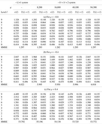
The result is summarized in Table B.1, which shows the optimal relativity, stationary distribution, and HMSE for each $\rho =-0.8,\ -0.4$, and $0.4$. Several comments are in place from this table:

• • For a given $\rho$ value, as $\varphi$ grows larger, the optimal relativities, stationary distribution, and HMSE become identical for both the $-1/+1$ and $-1/+1/+2$ BMSs. This is from a general property that, by definition, the $-1/+1/+2$ system with infinitely large threshold is the same as the $-1/+1$ system.

• • On the other hand, a smaller $\varphi$ means heavier penalty and more drivers end up in a higher BM level. This is confirmed by the stationary probability at the highest level ${\mathbb {P}}({L=9})$ growing larger as $\varphi$ decreases for all $\rho$ values. For $\rho =-0.8$ and $-0.4$, the threshold $\varphi$ at the 90th quantile shows the best performance in terms of the HMSE between four thresholds, whereas, in $\rho =0.4$ case, the 99th quantile is the best threshold. In general, the HMSE of the $-1/+1/+2$ system varies by the threshold and is not always smaller than that of the $-1/+1$ system. However, the best HMSE of the $-1/+1/+2$ system beats that of the $-1/+1$ system with an appropriate choice of the threshold $\varphi$, following the argument of Theorem 4. The optimal threshold can be found with numerical iterations, though its general solution is not straightforward.

• • As the dependence between frequency and individual severities becomes stronger, the aggregate severity becomes larger and the premium increase will be more substantial. We observe this from comparing the optimal relativities across different $\rho$ values. In particular, as $\rho$ becomes larger, the optimal relativities become larger for most BM levels with the exception in the lower BM levels, especially at level 0, in both the $-1/+1$ and $-1/+1/+2$ systems.

4.2. Impact of different mean frequency and transition rule

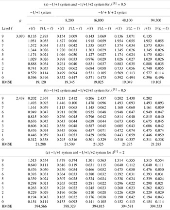
To study the impact of different frequency parameters and the transition rule, we consider several combinations on the mean frequency, whose result is shown in Table B.2, while other parameters are fixed at $\lambda ^{[2]}=\exp (8.8)$, $\psi ^{[2]}=1/0.67$, $(\sigma ^{[1]})^{2}=0.99$, and $(\sigma ^{[2]})^{2}=0.29$. For the dependence, we set $\rho =-0.45$, the choice made from an actual dataset in the next section.

• • In comparing (a) and (b) in Table B.2, we note that both keep the same frequency parameter $\lambda ^{[1]}$, but Table B.2(b) adopts a more stringent transition rule by having the $-1/+1/+3$ system. Consequently, the stationary probabilities ${\mathbb {P}}({L=\ell })$ in Table B.2(b) tend to be larger in the upper BM levels and smaller in the lower BM levels compared with Table B.2(a), as they should.

• • Furthermore, the best threshold among other alternatives in terms of the HMSE is $\varphi =16{,}800$ in Table B.2(a), but $\varphi =48{,}100$ in Table B.2(b). This implies that the optimal threshold depends on the transition rule as well as other parameters, as previously mentioned.

• • Table B.2(a) and (c) share the same transition rule but have different mean frequency $\lambda ^{[1]}$ values. By having a larger frequency mean, Table B.2(c) leads to a higher proportion of drivers in higher BM levels compared with Table B.2(a) under both the $-1/+1$ and $-1/+1/+2$ systems. However, the relativities are generally smaller in Table B.2(c) under both the BMS rules because of the negative $\rho$ value. That is, in this specific setting, the average claim size becomes smaller as there are more claims, and this, in turn, leads to a smaller aggregate loss on average. Similar to the above point, we also see that the optimal threshold in terms of the HMSE changes as $\lambda ^{[1]}$ does; for $\lambda ^{[1]}=0.5$, the optimal threshold is $\varphi =16{,}800$, corresponding to the 90th quantile, whereas $\varphi =94{,}300$, corresponding to the 99.9th quantile, when $\lambda ^{[1]}=2$.

4.3. Impact of different dependence among severities

Here, we study the impact of the dependence among individual severities by changing $\sigma ^{[2]}$. We assume the independence between frequency and individual severities by setting $\rho =0$ for this study. The other parameters are fixed at $\lambda ^{[1]}=0.5$, $\lambda ^{[2]}=\exp (8.8)$, $\psi ^{[2]}=1/0.67$, and $(\sigma ^{[1]})^{2}=0.99$.

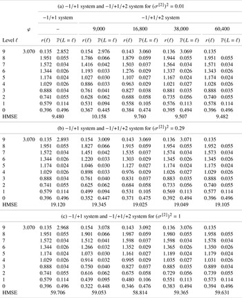
• • Focusing on the $-1/+1$ system, the optimal relativities remain the same over different $\sigma ^{[2]}$ values. This is because the $-1/+1$ system is driven by the frequency only and its relativities from the independence between frequency and severity; it responds to the mean $E( \Theta ^{[2]})$, but this mean is fixed at 1, although $\sigma ^{[2]}$ changes.

• • The independence between frequency and severity similarly affects the $-1/+1/+2$ system, where the stationary distribution stays the same over different $\sigma ^{[2]}$ values, which is justified from (19). However, the optimal relativities do change. In particular, the relativities become larger in higher BM levels as $\sigma ^{[2]}$ increases, for a given threshold $\varphi$. This occurs because a larger $\sigma ^{[2]}$ value yields larger claims.

• • As before, the optimal threshold varies as the $\sigma ^{[2]}$ value changes. For $(\sigma ^{[2]})^{2}=0.29$ and $1$, the optimal threshold in terms of the HMSE is found at the 90th quantile, whereas the optimal threshold is suggested to be much larger for $(\sigma ^{[2]})^{2}=0.01$.

5.1. Data description and estimation results

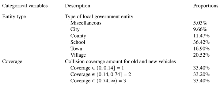
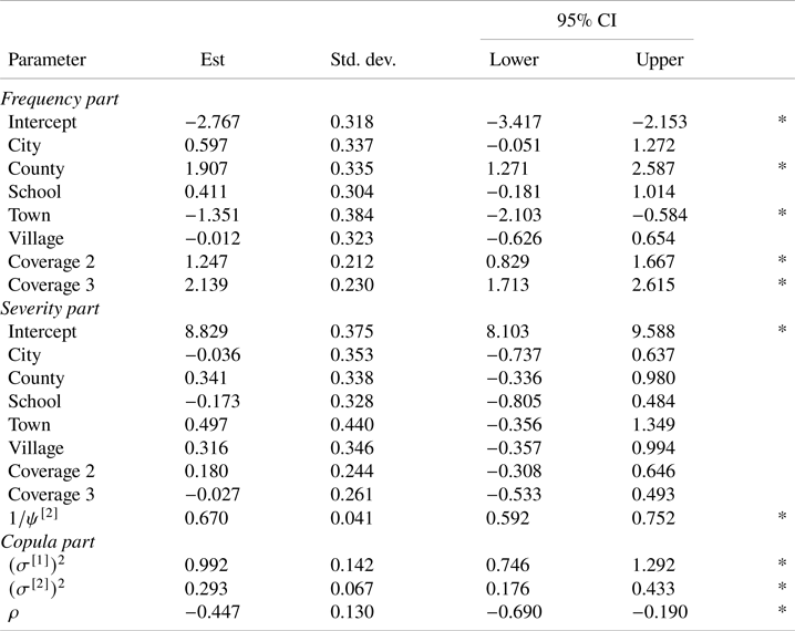
To examine the effect of the dependence on BM relativities, we now consider an actual insurance dataset concerning a collision coverage of new and old vehicles from the Wisconsin Local Government Property Insurance Fund (LGPIF) [Reference Frees, Lee and Yang8]. A detailed information on the project can be found at the LGPIF project website. The collision coverage provides cover for the impact of a vehicle with an object, impact of a vehicle with an attached vehicle, and overturn of a vehicle. The observations include policyholders who have either a new collision coverage, an old collision coverage, or both. In our analysis, longitudinal data over the policy years from 2006 to 2010 with 497 governmental entities are used. There are two categorical variables identical to the dataset studied in Oh et al. [Reference Oh, Shi and Ahn17]: the entity type with six levels and the coverage with three levels, as shown in Table B.4. Following this, we model the frequency part as

$$N_{t}\,|\,(\lambda_{\kappa}^{[1]}, \theta^{[1]})\sim \textrm{Poisson}(\lambda_\kappa^{[1]}\theta^{[1]})\quad \text{with} \ \lambda_\kappa^{[1]}=\exp(\boldsymbol{x}_\kappa^{[1]}\boldsymbol{\beta}^{[1]}),$$

and the individual severity part as

$$Y_{t,j}\,|\,(\lambda_{\kappa}^{[2]}, \theta^{[2]}) \sim \textrm{Gamma}(\lambda_\kappa^{[2]}\theta^{[2]},1/\psi^{[2]}) \quad \text{with} \ \lambda_\kappa^{[2]}=\exp(\boldsymbol{x}_\kappa^{[2]}\boldsymbol{\beta}^{[2]}),$$

where $\lambda _\kappa ^{[2]}\theta ^{[2]}$ is the mean and $1/\psi ^{[2]}$ is the shape parameter. In this data analysis, we use same a priori risk characteristics for both the frequency and severity parts, that is, $\boldsymbol {x}_\kappa ^{[1]}=\boldsymbol {x}_\kappa ^{[2]}$, and $\boldsymbol {\beta }^{[1]}$ and $\boldsymbol {\beta }^{[2]}$ are the corresponding regression coefficient vectors. For the bivariate random effect $(\Theta ^{[1]},\Theta ^{[2]})$, we assume bivariate Gaussian copula $C$ in (2) with the correlation coefficient $\rho$, and the Lognormal distributions with different parameters for the marginal distributions specified as

$$\Theta^{[1]} \sim \textrm{Lognormal}(-(\sigma^{[1]})^{2}/2, (\sigma^{[1]})^{2}) \quad \text{and} \quad \Theta^{[2]} \sim \textrm{Lognormal}(-(\sigma^{[2]})^{2}/2, (\sigma^{[2]})^{2}).$$

The estimation results of this model are summarized in Table B.5, and we refer to Oh et al. [Reference Oh, Shi and Ahn17] for further detailed estimation procedures. Note that $*$ sign indicates that the parameters whose 95$\%$ credible interval does not contain zero.

5.2. Optimal BM relativities in the modified BMS

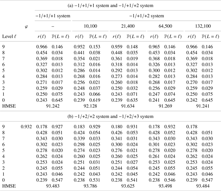
With the parameter estimates in Table B.5, the optimal BM relativities in (19) and the stationary distribution in (17) are calculated under four different BMSs. As per the threshold $\varphi$, we consider the estimated 75th, 90th, 99th, and 99.9th quantile of severity distribution, and the values of the HMSE are also provided to compare the performance. The results are summarized in Table B.6.

In Table B.6(a) and (b), the BMSs with $h_1=h_2$ are identical to those in Table B.2 of Oh et al. [Reference Oh, Shi and Ahn17]. Paying attention to the $-1/+1/+2$ and $-1/+2/+3$ systems, we note that:

• • As $\varphi$ decreases, the proportion of policyholders increases in higher BM levels and decreases in lower BM levels, as seen from the stationary distributions. This occurs because more drivers end up in high BM levels under smaller threshold $\varphi$. This tendency is naturally more pronounced for the $-1/+2/+3$ system compared with the $-1/+1/+2$ system, as the penalty under the former system is heavier.

• • Interestingly, the HMSEs of the optimal relativities under the $-1/+1/+2$ system are generally smaller than those under the $-1/+2/+3$ system for each given threshold. Though difficult to explain this in plain terms, we believe that the stationary distributions under the $-1/+1/+2$ system is more evenly spread than that under the $-1/+2/+3$ system, which, in turn, marginally stabilizes the BMS and produces smaller relativities. For the relationship between the stationary distribution and the optimal relativity, see Eqs. (19)–(21).

• • In terms of the HMSE, we see that the optimal threshold $\varphi$ must be quite large under both the $-1/+1/+2$ and $-1/+2/+3$ systems in this particular dataset.

Overall, based on the HMSE criterion, we would recommend the $-1/+1/+2$ transition rule with a highest threshold $\varphi$, the 99.9th quantile, as a new BMS of choice; different datasets may lead to different optimal thresholds. Though the improvement in the HMSE may seem marginal compared with the frequency-driven BMS case in this dataset, the actual amount of dollar saved can be substantial for insurers with large auto portfolios.