


%20--%3e%3c!DOCTYPE%20svg%20PUBLIC%20'-//W3C//DTD%20SVG%201.0//EN'%20'http://www.w3.org/TR/2001/REC-SVG-20010904/DTD/svg10.dtd'%3e%3csvg%20version='1.0'%20id='Layer_1'%20xmlns='http://www.w3.org/2000/svg'%20xmlns:xlink='http://www.w3.org/1999/xlink'%20x='0px'%20y='0px'%20width='64px'%20height='64px'%20viewBox='5.5%20-3.5%2064%2064'%20enable-background='new%205.5%20-3.5%2064%2064'%20xml:space='preserve'%3e%3cg%3e%3ccircle%20fill='%23FFFFFF'%20fill-opacity='0'%20cx='37.785'%20cy='28.501'%20r='28.836'/%3e%3cpath%20fill='%23595959'%20d='M37.441-3.5c8.951,0,16.572,3.125,22.857,9.372c3.008,3.009,5.295,6.448,6.857,10.314%20c1.561,3.867,2.344,7.971,2.344,12.314c0,4.381-0.773,8.486-2.314,12.313c-1.543,3.828-3.82,7.21-6.828,10.143%20c-3.123,3.085-6.666,5.448-10.629,7.086c-3.961,1.638-8.057,2.457-12.285,2.457s-8.276-0.808-12.143-2.429%20c-3.866-1.618-7.333-3.961-10.4-7.027c-3.067-3.066-5.4-6.524-7-10.372S5.5,32.767,5.5,28.5c0-4.229,0.809-8.295,2.428-12.2%20c1.619-3.905,3.972-7.4,7.057-10.486C21.08-0.394,28.565-3.5,37.441-3.5z%20M37.557,2.272c-7.314,0-13.467,2.553-18.458,7.657%20c-2.515,2.553-4.448,5.419-5.8,8.6c-1.354,3.181-2.029,6.505-2.029,9.972c0,3.429,0.675,6.734,2.029,9.913%20c1.353,3.183,3.285,6.021,5.8,8.516c2.514,2.496,5.351,4.399,8.515,5.715c3.161,1.314,6.476,1.971,9.943,1.971%20c3.428,0,6.75-0.665,9.973-1.999c3.219-1.335,6.121-3.257,8.713-5.771c4.99-4.876,7.484-10.99,7.484-18.344%20c0-3.543-0.648-6.895-1.943-10.057c-1.293-3.162-3.18-5.98-5.654-8.458C50.984,4.844,44.795,2.272,37.557,2.272z%20M37.156,23.187%20l-4.287,2.229c-0.458-0.951-1.019-1.619-1.685-2c-0.667-0.38-1.286-0.571-1.858-0.571c-2.856,0-4.286,1.885-4.286,5.657%20c0,1.714,0.362,3.084,1.085,4.113c0.724,1.029,1.791,1.544,3.201,1.544c1.867,0,3.181-0.915,3.944-2.743l3.942,2%20c-0.838,1.563-2,2.791-3.486,3.686c-1.484,0.896-3.123,1.343-4.914,1.343c-2.857,0-5.163-0.875-6.915-2.629%20c-1.752-1.752-2.628-4.19-2.628-7.313c0-3.048,0.886-5.466,2.657-7.257c1.771-1.79,4.009-2.686,6.715-2.686%20C32.604,18.558,35.441,20.101,37.156,23.187z%20M55.613,23.187l-4.229,2.229c-0.457-0.951-1.02-1.619-1.686-2%20c-0.668-0.38-1.307-0.571-1.914-0.571c-2.857,0-4.287,1.885-4.287,5.657c0,1.714,0.363,3.084,1.086,4.113%20c0.723,1.029,1.789,1.544,3.201,1.544c1.865,0,3.18-0.915,3.941-2.743l4,2c-0.875,1.563-2.057,2.791-3.541,3.686%20c-1.486,0.896-3.105,1.343-4.857,1.343c-2.896,0-5.209-0.875-6.941-2.629c-1.736-1.752-2.602-4.19-2.602-7.313%20c0-3.048,0.885-5.466,2.658-7.257c1.77-1.79,4.008-2.686,6.713-2.686C51.117,18.558,53.938,20.101,55.613,23.187z'/%3e%3c/g%3e%3c/svg%3e)
%20--%3e%3c!DOCTYPE%20svg%20PUBLIC%20'-//W3C//DTD%20SVG%201.0//EN'%20'http://www.w3.org/TR/2001/REC-SVG-20010904/DTD/svg10.dtd'%3e%3csvg%20version='1.0'%20id='Layer_1'%20xmlns='http://www.w3.org/2000/svg'%20xmlns:xlink='http://www.w3.org/1999/xlink'%20x='0px'%20y='0px'%20width='64px'%20height='64px'%20viewBox='5.5%20-3.5%2064%2064'%20enable-background='new%205.5%20-3.5%2064%2064'%20xml:space='preserve'%3e%3cg%3e%3ccircle%20fill='%23FFFFFF'%20fill-opacity='0'%20cx='37.637'%20cy='28.806'%20r='28.276'/%3e%3cg%3e%3cpath%20fill='%23595959'%20d='M37.443-3.5c8.988,0,16.57,3.085,22.742,9.257C66.393,11.967,69.5,19.548,69.5,28.5c0,8.991-3.049,16.476-9.145,22.456%20C53.879,57.319,46.242,60.5,37.443,60.5c-8.649,0-16.153-3.144-22.514-9.43C8.644,44.784,5.5,37.262,5.5,28.5%20c0-8.761,3.144-16.342,9.429-22.742C21.101-0.415,28.604-3.5,37.443-3.5z%20M37.557,2.272c-7.276,0-13.428,2.553-18.457,7.657%20c-5.22,5.334-7.829,11.525-7.829,18.572c0,7.086,2.59,13.22,7.77,18.398c5.181,5.182,11.352,7.771,18.514,7.771%20c7.123,0,13.334-2.607,18.629-7.828c5.029-4.838,7.543-10.952,7.543-18.343c0-7.276-2.553-13.465-7.656-18.571%20C50.967,4.824,44.795,2.272,37.557,2.272z%20M46.129,20.557v13.085h-3.656v15.542h-9.944V33.643h-3.656V20.557%20c0-0.572,0.2-1.057,0.599-1.457c0.401-0.399,0.887-0.6,1.457-0.6h13.144c0.533,0,1.01,0.2,1.428,0.6%20C45.918,19.5,46.129,19.986,46.129,20.557z%20M33.042,12.329c0-3.008,1.485-4.514,4.458-4.514s4.457,1.504,4.457,4.514%20c0,2.971-1.486,4.457-4.457,4.457S33.042,15.3,33.042,12.329z'/%3e%3c/g%3e%3c/g%3e%3c/svg%3e)
%20--%3e%3c!DOCTYPE%20svg%20PUBLIC%20'-//W3C//DTD%20SVG%201.0//EN'%20'http://www.w3.org/TR/2001/REC-SVG-20010904/DTD/svg10.dtd'%3e%3csvg%20version='1.0'%20id='Layer_1'%20xmlns='http://www.w3.org/2000/svg'%20xmlns:xlink='http://www.w3.org/1999/xlink'%20x='0px'%20y='0px'%20width='64px'%20height='64px'%20viewBox='5.5%20-3.5%2064%2064'%20enable-background='new%205.5%20-3.5%2064%2064'%20xml:space='preserve'%3e%3cg%3e%3ccircle%20fill='%23FFFFFF'%20fill-opacity='0'%20cx='36.924'%20cy='28.403'%20r='28.895'/%3e%3cpath%20fill='%23595959'%20d='M37.442-3.5c8.99,0,16.571,3.085,22.743,9.256C66.393,11.928,69.5,19.509,69.5,28.5c0,8.992-3.048,16.476-9.145,22.458%20C53.88,57.32,46.241,60.5,37.442,60.5c-8.686,0-16.19-3.162-22.513-9.485C8.644,44.728,5.5,37.225,5.5,28.5%20c0-8.762,3.144-16.343,9.429-22.743C21.1-0.414,28.604-3.5,37.442-3.5z%20M12.7,19.872c-0.952,2.628-1.429,5.505-1.429,8.629%20c0,7.086,2.59,13.22,7.77,18.4c5.219,5.144,11.391,7.715,18.514,7.715c7.201,0,13.409-2.608,18.63-7.829%20c1.867-1.79,3.332-3.657,4.398-5.602l-12.056-5.371c-0.421,2.02-1.439,3.667-3.057,4.942c-1.622,1.276-3.535,2.011-5.744,2.2%20v4.915h-3.714v-4.915c-3.543-0.036-6.782-1.312-9.714-3.827l4.4-4.457c2.094,1.942,4.476,2.913,7.143,2.913%20c1.104,0,2.048-0.246,2.83-0.743c0.78-0.494,1.172-1.312,1.172-2.457c0-0.801-0.287-1.448-0.858-1.943l-3.085-1.315l-3.771-1.715%20l-5.086-2.229L12.7,19.872z%20M37.557,2.214c-7.276,0-13.428,2.571-18.457,7.714c-1.258,1.258-2.439,2.686-3.543,4.287L27.786,19.7%20c0.533-1.676,1.542-3.019,3.029-4.028c1.484-1.009,3.218-1.571,5.2-1.686V9.071h3.715v4.915c2.934,0.153,5.6,1.143,8,2.971%20l-4.172,4.286c-1.793-1.257-3.619-1.885-5.486-1.885c-0.991,0-1.876,0.191-2.656,0.571c-0.781,0.381-1.172,1.029-1.172,1.943%20c0,0.267,0.095,0.533,0.285,0.8l4.057,1.83l2.8,1.257l5.144,2.285l16.397,7.314c0.535-2.248,0.801-4.533,0.801-6.857%20c0-7.353-2.552-13.543-7.656-18.573C51.005,4.785,44.831,2.214,37.557,2.214z'/%3e%3c/g%3e%3c/svg%3e)
%20--%3e%3c!DOCTYPE%20svg%20PUBLIC%20'-//W3C//DTD%20SVG%201.1//EN'%20'http://www.w3.org/Graphics/SVG/1.1/DTD/svg11.dtd'%3e%3csvg%20version='1.1'%20id='Layer_1'%20xmlns='http://www.w3.org/2000/svg'%20xmlns:xlink='http://www.w3.org/1999/xlink'%20x='0px'%20y='0px'%20width='64.000977px'%20height='64px'%20viewBox='0%200%2064.000977%2064'%20enable-background='new%200%200%2064.000977%2064'%20xml:space='preserve'%3e%3cg%3e%3ccircle%20fill='%23FFFFFF'%20fill-opacity='0'%20cx='32.064453'%20cy='31.788086'%20r='29.012695'/%3e%3cg%3e%3cpath%20fill='%23595959'%20d='M31.943848,0C40.896484,0,48.476562,3.105469,54.6875,9.314453C60.894531,15.486328,64.000977,23.045898,64.000977,32%20s-3.048828,16.457031-9.145508,22.513672C48.417969,60.837891,40.779297,64,31.942871,64%20c-8.648926,0-16.152832-3.142578-22.513672-9.429688C3.144043,48.286133,0,40.761719,0,32.000977%20c0-8.723633,3.144043-16.285156,9.429199-22.68457C15.640137,3.105469,23.14502,0,31.943848,0z%20M32.060547,5.771484%20c-7.275391,0-13.429688,2.570312-18.458496,7.714844C8.381836,18.783203,5.772949,24.954102,5.772949,32%20c0,7.125,2.589844,13.256836,7.77002,18.400391c5.181152,5.181641,11.352051,7.770508,18.515625,7.770508%20c7.123047,0,13.332031-2.608398,18.626953-7.828125C55.713867,45.466797,58.228516,39.353516,58.228516,32%20c0-7.3125-2.553711-13.484375-7.65625-18.513672C45.504883,8.341797,39.333984,5.771484,32.060547,5.771484z%20M44.117188,24.456055%20v5.485352H20.859863v-5.485352H44.117188z%20M44.117188,34.743164v5.481445H20.859863v-5.481445H44.117188z'/%3e%3c/g%3e%3c/g%3e%3c/svg%3e)
1. Introduction and background
Following Reference GrievesGrieves (2015) seminal whitepaper describing the Digital Twin (DT) Academic publications on DTs have grown at an average rate of 47% per year between 2015 and 2025 (Scopus). This academic enthusiasm is mirrored in market predictions. The Digital Twin industry is expected to grow from a current valuation of £14.38B to £210.36B by 2032, a compound annual growth rate of 39.8% (Reference InsightsInsights, 2025). Interest from technical leads in industry share this sentiment with 59% of executives across various industries planning to integrate Digital Twins (Businesswire, 2023), while 70% of c-suite technology executives are actively exploring or investing in Digital Twin technology (Mckinsey, 2022). A 2024 industry study surveyed 660 C-level executives across 11 industries and found that 91% of respondents were planning to maintain or increase their investment in Digital Twins in the coming year, and 72% were planning to increase their spending in this area (Hexagon, 2024). In the same study, 75% of respondents who claimed that they were very familiar with Digital Twins thought that they could deliver significant value for their organisation. Despite the enthusiasm and market expectancy, there exist few methodologies and tools to support firms in designing their Digital Twin and subsequent investment strategy to realise it. The majority of support to date comes through consultancy projects with DT experts. Cost estimate heuristics vary widely during the concept design stage, highlighting the financial challenge. The development of the core Digital Twin software platform alone, not including hardware, data connections, or simulation models, is estimated to be $20,000 to $45,000 for a small company, rising to between $75,000 and $90,000 for large enterprises (RisingMax, 2024). More holistic estimates, which include all elements (sensing, communication, simulation, intervention) of the DT, range from $300,000 for a Digital Twin of a distribution centre, to between $4 million and $5.6 million for a complex physical entity such as a shopping centre (Lengthorn, n.d.). It can be particularly difficult to estimate the total cost of a Digital Twin project at the early conceptual design stages leading to uncertainty around investment, resulting in delayed or slow adoption (Reference Mihai, Yaqoob, Hung, Davis, Towakel, Raza, Karamanoglu, Barn, Shetve, Prasad, Venkataraman, Trestian and NguyenMihai et al., 2022).
Traditional methods for undertaking investment decisions, are not sufficient to understand the cost-benefit proposition of DTs. Techniques such as Net Present Value or Internal Rate of Return typically treat the project as a monolithic capital expenditure (Capex) with predictable returns (Reference BrealeyBrealey, 2023). These approaches fail to capture the emergent nature of the return of a DT, and the interconnected nature of the cost drivers of the many assets that form a DT and the benefits they provide and contribute to. Analysis of the economics of DTs highlights that characterising the full spectrum of costs and benefits is a significant challenge, with benefits often embedded in operational processes, making it difficult to assign value (Reference ThomasThomas, 2024). The constituent elements of a DT are a mixture of Capital Expenditures (CapEx), and ongoing Operational Expenditure (OpEx) costs, which can vary greatly, and scale non-linearly with the number of assets, data fidelity and model complexity (Reference McClenaghan, Gopsill, Ballantyne and HicksMcClenaghan et al., 2023).
DTs are emergent in nature, they can be implemented over time with new sensors, databases, and feedback mechanisms being added. At the early concept stage, it is beneficial to be able to map out the entire space, which can then be queried to define the elements that offer the greatest cost-benefit proposition to the company.
This paper contributes to the design of Digital Twins by providing a schema that augments existing DT network architecture modelling practices with the cost information necessary to evaluate costs at the concept stage. The paper continues by summarising related work, including existing cost estimation techniques that serve as inputs to any financial model and the uses of graphs in engineering in Section 2, followed by presenting the schema and the methodology used to derive it in Section 3. Analysis metrics for the schema are presented in Section 4, with a worked example demonstrating their use shown in Section 5. Finally, Section 6 discusses the implications, advantages, and limitations of this approach, concluding with directions for future work.
2. Related work
This section presents existing costing methodologies, and the drawbacks of each. It then follows with an examination of how graphs are used in the engineering field to represent systems before introducing schemas, and the benefits they provide when applied to graphs of this nature.
2.1. Costing methodologies
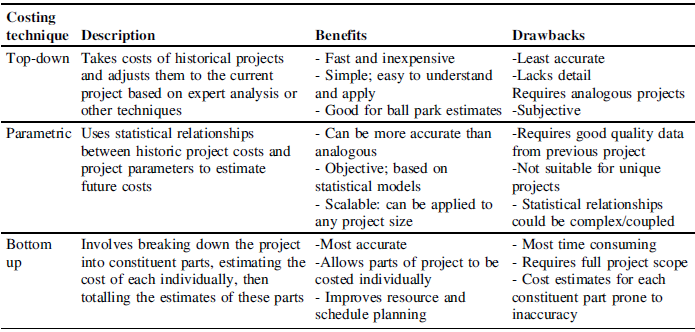
There are three main categories of cost estimation techniques, analogous (Top down) methods, parametric methods, and bottom up methods, also called “grassroots” methods (NASA, 2023). Table 1 provides a description, and a summary of the benefits and drawbacks of each technique.
Overview of costing techniques

This bottom up approach is well suited to the modular nature of a Digital Twin, however a simple aggregation of parts fails to capture the interdependencies and non-linear scaling effects inherent in DTs. To extend this bottom-up approach and enable a full cost-benefit analysis (CBA), this paper proposes that the costs and benefits can be represented through a directed, attributed graph.
2.2. Graphs in the design of engineering systems and digital twins
A DT is a system, a combination of interacting elements organized to achieve one or more stated outcomes, (International Organization for Standardization et al., 2023). An intuitive way of modelling systems is a graph consisting of nodes that represent system elements and edges representing the relationships between them (Reference Heckmann, Schwanghart and PhillipsHeckmann et al., 2014). The use of graphs for the representation of engineering systems is a mature area of research, with applications in fields such as electrical circuit analysis, modelling transport systems, and signal flow, among many others (Reference DeoDeo, 1974). In the costing space, the benefits of graphs are being increasingly utilised; Reference Khan, Matskin, Prodan, Bussler, Roman and SoyluKhan et al. (2024) used them to calculate and optimise the cost of cloud infrastructure, while Reference Guo, Tian, Jiang and WangGuo et al. (2018) utilised graphs to model the costs of changes to supply chains.
To effectively represent Digital Twins in this way, a directed multi-graph is required, which has a direction constraint placed on edges, and multiple possible edges between nodes. More detail of the mathematical foundations of graphs of this type can be found in (Reference DiestelDiestel, 2018).
Graphs of engineering systems typically adhere to defined schemas that enable analysis of the complex technical correlations within a system, and efficient storage in databases (Reference Patzwahl and HybaPatzwahl & Hyba, 2022). A schema is a set of rules that governs how data is organised, named, and how different pieces of data relate to one another. Examples include JSON (Reference Pezoa, Reutter, Suarez, Ugarte and VrgočPezoa et al., 2016), GraphML (Reference Brandes, Eiglsperger, Herman, Himsolt, Marshall, Mutzel, Jünger and LeipertBrandes et al., 2002), GML (Reference HimsoltHimsolt, 2010). Schemas such as these enables data consistency, validity and interoperability for data. In contrast, architecture diagrams for DTs at the conceptual stage remain largely visual with ad-hoc unstructured annotations. It is often only at the embodiment design stage where more structured schemas, such as UML, are used to define the interfaces between assets within a DT.
3. Schema
This section details the proposed cost schema to augment existing DT architectural network design practices with cost information in a structured manner that can be subsequently used to provide insights and forecast the cost of a DT deployment earlier in the design stage.
3.1. Schema development
In literature, DTs are typically presented in the form of an architecture diagram that depicts the key services and data flow(s). To translate these architectures to graphs representations that can be used for cost analysis, a schema is required to govern the types of nodes, edges, and required parameters for each.
To establish the requirements for the schema, we searched Scopus for publications that contained holistic Digital Twin architectures. The search resulted in 10 papers that presented complete representations of their architecture. We then extracted the necessary detail and synthesised them into simplified representations, containing all nodes, and representative edges connecting them. Two examples of the outputs of this process can be seen in Figure 1. From these graphs, we derived an initial schema containing the minimum set of node types that could represent the graphs. Through a series of iterations, we refined the schema until it captured all the necessary information and could represent all the presented architectures completely. In the remainder of Section 3 we define the final schema produced in this process.
Examples of adaptations of architectures from literature, (a) adapted from Reference Gürdür Broo, Bravo-Haro and SchoolingGürdür Broo et al. (2022), (b) adapted from Reference Alonso, Locci and RecuperoAlonso et al. (2024)

3.2. Node schema
Through the iteration of the schema, we determined that all architectures could be represented by a graph containing four node types: 1) Source; 2) Sink; 3) Store, and, 4) Transformer.
All four node types inherit a base node definition (Figure 2(a)), which describes attributes that all nodes have in common. Every node has an id, an optional name and description, an active Boolean and an associated cost function. The active Boolean determines whether that node is included in the costing calculations. This is utilised when isolating data streams to examine the cost-benefit proposition of different Digital Twin outputs. One of the key findings from the review of architectures and cost elements is that the costs can all be modelled by a function, parameterised by the size and frequency of data entering the node. This cost function also encapsulates the costs incurred by transferring data between nodes. The schema places no constraints on the structure of the cost function as it will be dependent on the context that node represents, however it will be a function of the size and frequency of the data flowing into the node and will return data in the form of a Cost, the definition of which is shown in Figure 2(b). The function will have access to the node’s context and must be defined.
3.2.1. Source
A source is a point at which data enters the DT. It is defined in the schema as a node that has a data output, but no data input. Examples of sources could include sensors, connections to external APIs to get information, human input from a technician, as well as data from a manufacturing machine such as a 3D printer. The class definition for a source can be seen in Figure 2(c). The send attribute is a list, to allow the source to send data to multiple nodes, to send multiple pieces of data to one node, or a combination of the two. The one-to-many mapping of data out to another node would allow for the situation where a sensor is producing multiple data types, as each data edge specifies one piece of data. An example of this would be an accelerometer, sending x, y, z data. In this scenario, the accelerometer would be represented as a single source, however each piece of data out would be carried along its own edge to its respective destination.
3.2.2. Sink
A sink is a point at which data exits the DT and provides a useful output outside of the DT, allowing value to be derived from the data that enters the sink. It represents an output of the graph and is defined as a node that receives information, does not produce any, and enables the realisation of a benefit from the information it receives. Examples of sinks could be a dashboard, an email notification service, or an automated intervention that happens based on the data it receives. The sink class includes a benefits attribute, which can be used to assign benefits to the sink, such as a percentage throughput improvement, or a reduction in the number of defective parts. The class definition of a sink can be seen in Figure 2(d).
3.2.3. Store
A store node is defined as a node that both receives and produces data but does not manipulate the data. The cost function of the Store node captures the cost of holding data in that node. The send and receive attributes contain lists that define the edges into and out of each node. The class definition of a Store can be seen in Figure 2(e). Examples of stores include Data Lakes, Databases and Blob Stores.
3.2.4. Transformer
A transformer is any node that receives and produces data and performs some manipulation on that data. The manipulation performed is not defined in the schema at this stage, but the cost of the manipulation is captured in the cost function, inherited from the base node class. Examples of transformers include a simulation running in a cloud based virtual machine, or a serverless cloud computation instance that is activated to clean data before it is passed to another element. Each Transformer has an attribute for send and receive, each containing a list of all the edges into and out of the node. The class definition can be seen in Figure 2(f).
Base node and cost (a,b) and node definitions (c-f)

3.3. Edge schema
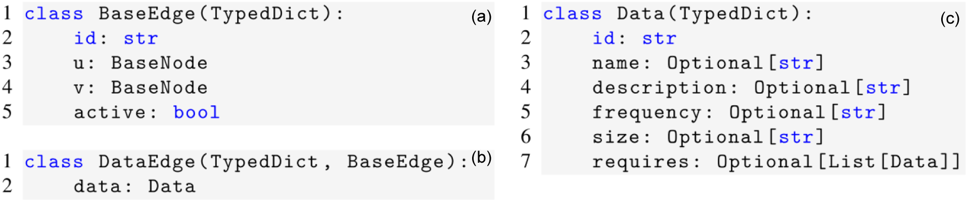
With the nodes defined, the schema must now define the connections between them. In the same way as the node schema, the edge schema begins with a base edge class, as can be seen in Figure 3(a). The base edge contains an id attribute, an active attribute, which behaves in the same way as this attribute of Base Node, and u and v attributes, which define the start and end nodes respectively.
Inheriting from the Base Edge class is the Data Edge.
3.3.1. Data edge
The data edge defines a connection where data is being transferred between two nodes. The class definition can be seen in Figure 3(b). Since DataEdge inherits its start and end nodes from the BaseEdge class, the only attribute is data, which defines the data passed along the edge. This data is governed by the Data class, as can be seen in Figure 3(c). The data class contains an id attribute, to allow that piece of data to be traced throughout the graph, as well as optional name and description attributes. It also includes metadata describing the underlying data; its frequency, how often that piece of data is transferred along that edge, and the size, the size of each piece of data being transferred. The class also includes a requires attribute. This attribute is used for traceability of data through the graph. An example of its use would be if temperature data was passed to a transformer representing a Finite Element analysis used to calculate thermal expansion. The thermal expansion data instance, that was the output data of that transformer, would list temperature in its required attribute.
Base edge definition (a), data edge definition (b), and data attribute definition (b)

3.4. Global rules
Beyond the definition of nodes and edges, there are several rules that are applied globally to ensure that the graph representation is valid. A valid graph means that all nodes obey the class definitions previously presented and that the following rules are adhered to:
-
1. All data produced by a source must terminate at one or more stores or sinks, or be transformed within a transformer.
-
2. The graph must be acyclic. This means that a type of data must either be transformed, stored, or sunk; there can be no cycles.
Rule 1 ensures that all data produced by sources is used in some form or another. If a source produces data that is not utilised anywhere else in the graph, this data should not be included in the analysis. It is valid for data to be produced and terminate in a store, as this may be the case for incremental development of a DT, data might be collected now, and stored for future processing, but the data cannot be produced and go nowhere. Rule 2 necessitates an acyclic graph, this is to prevent infinite loops where a piece of data is perpetually moved in a cycle, without being utilised elsewhere. From a pragmatic standpoint, this constraint is essential for the stability of the cost algorithm presented in Section 4 as the presence of cycles would render the recursive calculations intractable.
4. Cost analysis at the conceptual design phase
This section details the proposed analysis methodologies that this schema will allow, before a vision demonstrator is presented in Section 5.
4.1. Path isolation
Sub-graphs can be generated that includes only the nodes and edges that directly contribute to a given sink node, enabling analysis of per-benefit cost calculations. The approach takes a directed graph of the entire DT, G and a target sink t as inputs. It then finds the set R of all ancestor nodes of t in the graph. An ancestor node is any node that has a directed path of any length to the target node. A sub-graph of 𝐺 is then created, which includes only the nodes in 𝑅, as well as the target node t. The sub-graph includes all edges from G that connect the nodes in R. The pseudocode for this approach can be seen in Figure 4. The Benefit score associated with that sink is taken as the benefit side of the analysis, and the costs of the subset of the graph associated with that sink is compared against it. To consider multiple outputs simultaneously, the union of multiple subgraphs can be taken.
Algorithm to get subgraph for target node

4.2. Cost calculation
Each node in the graph has an associated cost attribute, which is defined as a function that returns a cost value for a given period. To establish the cost of a specific output, represented by a sink, the subset of the overall DT that contributes to that sink is identified using the path isolation algorithm. The cost calculation methodology traverses the path between nodes and calls the cost function of each visited node. This cost function increments a global cost counter. An overview of the algorithm to achieve this is shown in Figure 5.
By repeating this process for different graph configurations, designers can perform a comparative Cost Analysis between proposed options, allowing the design of the DT to be optimised before any physical implementation. A designer could also examine the impact of altering the parameters of elements of the DT, such as sensing rate or fidelity of a source, by calculating the downstream impact on the total cost of a specific sink node. Alternatively, when combined with the benefits assigned to each sink node, the cost-benefit trade-off of adding new elements to the DT could also be investigated, and the order of their implementation optimised to maximise the benefit accrued for each element added to the design.
To account for the uncertainty in early-stage design, probabilistic approaches could also be incorporated, to improve the accuracy of cost estimates. By assigning a probability distribution to each parameter, or to the output of the cost function, these distributions can be randomly sampled, forming a Monte-Carlo analysis to produce and overall probability distribution for the resultant cost.
Cost calculation algorithm

5. Worked example
To demonstrate the schema in the design process for a Digital Twin, it will now be applied to a hypothetical case study that was produced using knowledge from the review of architecture during the development of the schema. The scenario for this case study is that a proposed DT design is being assessed for viability. The physical entity in this case study is a 3D printer, and the outputs are a predictor of the printer’s next state, an email notification service to notify a technician that the print is complete, a report generator, and a delta between the bed temperature and the target bed temperature. Using the presented schema, this case study is represented as a graph in Figure 6. The labels on each edge represent the name of the data object associated with that edge.
Case study architecture represented as a graph

To conduct the analysis, the graph was built using the networkx package for python, with nodes and edges created in accordance with the class definitions presented in Section 3. Each node contained attributes for each of the parameters outlined in its definition in Section 3. For the purposes of this example the cost function of each node was set as a constant, these are summarised in Table 2, along with illustrative benefits assigned to each output.
Illustrative costs for nodes

Using the path isolation algorithm detailed in Figure 4, the sub-graphs pertaining to the Report generation sink (RG), the State Prediction Sink (SP) and the Temp Dashboard Sink (TD) can be identified, and are shown in Figure 7 (a), (b), and (c) respectively.
Sub-graph for each sink

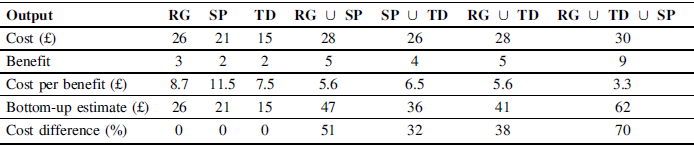
The costs for each subgraph are calculated using the costing algorithm detailed in Figure 5, combined with the costs defined in Table 2, the results are shown in Table 3. For design options with multiple outputs, the cost estimate is compared to a bottom-up estimate, which involves aggregating the cost of each output individually.
Comparison of costs of different outputs from the worked example

The percentage differences between the estimate approaches demonstrates that traditional bottom-up approaches significantly overestimate the cost of implementation of these features when the estimate contains multiple outputs. This demonstrates that traditional methods fail to account for the interconnected nature of DTs and the benefits of using a graph-based approach. The cost per benefit score indicates the trade-off between cost and benefit in this case and can help to prioritise implementation to achieve an optimal implementation order. This analysis is summarised in Table 4, and shows that an optimal implementation order of
 $$TD \to RG \to SP$$
can be deduced.
Optimal implementation order for worked example

6. Discussion and conclusions
The primary contribution of this work is the formalisation and extension of a DT architecture into a computable, algorithmically queryable topology. This representation through a formal graph schema provides a direct solution to the key challenges of DT cost analysis, particularly the problem of evaluating and attributing interconnected costs. As demonstrated through the worked example, bottom-up summations can provide overestimates of costs, as they fail to account for shared uses of nodes. It showed that bottom-up estimate, which aggregates the cost of individual outputs, overestimated the total cost by up to 70% for a system with three outputs (RG ∪ TD ∪ SP). This overestimation could be particularly prevalent in situations where siloed teams are developing components of the DT separately. The holistic graph representation allows opportunities for consolidation and therefore cost reduction to become apparent. The analysis framework provides better understanding of the marginal cost of adding new features and can help to identify areas where existing capabilities to be leveraged to achieve more benefits in the form of new outputs. Table 4 demonstrates that these capabilities can be utilised to determine an optimal implementation order, that maximises the cost-benefit proposition at each stage of the process.
Beyond costing, this form of representation can be used for overall systems analysis. The path isolation algorithm presented in Figure 4 can be used for impact analysis, looking at the propagation of failures if a node were to become inoperable, and identification of optimisation opportunities beyond pure cost optimisation.
There are several limitations to the current work, which in turn define the path for future research. The first limitation is that while the paper proposes a schema that can be used for full Cost-benefit analysis, it only provides a fully realised methodology for cost-estimation. The worked example includes indicative benefits, however, the methodology for quantifying these benefits and assigning them to specific business functions is an ongoing avenue of future work. To characterise the benefits and attribute them to Sink nodes, the future work will involve developing a database of benefits, and a ranking or weighting system to assign them as numerical values to the sink nodes, similar to the indicative values assigned in Section 5. Extensions to the schema to include dedicated nodes capturing these benefits are another possibility to be explored.
Another limitation is that the cost function attributed to each BaseNode, Figure 3(a), is currently presented as a node-specific black box. This paper proposed the framework and return type for these functions but did not define their specific structure. The practical implementation of this framework hinges on defining realistic cost functions for each node. This is another important area of future work and will involve empirical studies of real-world DT components to create a catalogue of standardised, parameter-driven cost functions. Another area of future work in this area is the implementation of probabilistic costing. This would be valuable as it would allow the appraisal of the potential range and uncertainty of the project.
The worked example utilised in this study is a relatively simple scenario. While useful for demonstrating the techniques presented, it does not accurately reflect the size and complexity of industrial DTs. Investigation of the schema’s scalability and performance with highly complex DTs with large numbers of nodes, and intricate interdependencies is another important area of future work.
The schema presented in this work is designed to be used in the early stages of the design cycle, to determine an estimate of the cost-benefit proposition of potential DT projects. The paper has presented proposed analysis techniques to utilise the structure of the schema to calculate cost estimates for proposed architectures, and compare them to a metric quantifying the benefits. The analysis of the proposed architecture demonstrates the importance of considering costs as a union of services, rather than costs in isolation. The schema presented is sector agnostic, in that it can represent a DT for any purpose, and allows for iteration of multiple architecture concepts to decide on the optimal structure for a proposed Digital Twin.








 Open access

