





1. Introduction
Spectropolarimetric inversions are a fundamental tool for studying the solar atmosphere by analyzing the light we observe from the sun. This light is characterized by its raw intensity and the polarization states that are all described by the so-called Stokes parameters I, Q, U, and V. By means of spectropolarimetric analysis, we can decode the fingerprints encoded by the physical behavior of the solar atmosphere in the emitted light (del Toro Iniesta and Ruiz Cobo Reference del Toro Iniesta and Ruiz Cobo2016). There are various techniques for performing spectropolarimetry, but all of them are based on the same concept of inversion of the Radiative Transfer Equation (RTE), which is the general model that describes how light interacts with a medium (del Toro Iniesta and Ruiz Cobo Reference del Toro Iniesta and Ruiz Cobo2016; del Toro Iniesta Reference del Toro Iniesta2007; Chandrasekhar Reference Chandrasekhar1960). Diverse algorithms have been developed to solve the inversion problem, ranging from numerical methods that assume local thermodynamic equilibrium (LTE) to non-local thermodynamic equilibrium (NLTE) (del Toro Iniesta and Ruiz Cobo Reference del Toro Iniesta and Ruiz Cobo2016). Since these methods tend to be too computationally demanding, in addition to having unrealistic processing times for scientific development, new techniques involving technologies such as Machine Learning models have been developed (Mistryukova et al. Reference Mistryukova, Plotnikov, Khizhik, Knyazeva, Hushchyn and Derkach2023; Asensio Ramos et al. Reference Asensio Ramos, Cheung, Chifu and Gafeira2023a).
Recent advances in artificial intelligence and machine learning technology have not left the solar physics community indifferent. Various kinds of applications of Machine Learning algorithms have been implemented in recent years, including superresolution models, forecasting algorithms, classification of features in the solar atmosphere at different heights, and segmentation, among others Asensio Ramos et al. (Reference Asensio Ramos, Cheung, Chifu and Gafeira2023b). For the topic that concerns this work, Machine learning algorithms have also been applied for spectropolarimetric inversions. These algorithms vary from simple, deeply connected neural networks that are used for generation or classification, such as the first ever published work on deep learning inversions from Carroll and Staude (Reference Carroll and Staude2001), to different models that apply convolutions (Asensio Ramos and D az Baso 2019; Milić and Gafeira Reference Milić and Gafeira2020; Gafeira et al. Reference Gafeira, Orozco Suárez, Milić, Quintero Noda, Ruiz Cobo and Uitenbroek2021), invertible models (Osborne et al. Reference Osborne, Armstrong and Fletcher2019), and even the application of uncertainty generation (Higgins et al. Reference Higgins, Fouhey, Zhang, Antiochos, Barnes, Hoeksema, Leka, Liu, Schuck and Gombosi2021; Mistryukova et al. Reference Mistryukova, Plotnikov, Khizhik, Knyazeva, Hushchyn and Derkach2023).
Continuing this approach, this work aims to create a one dimensional model that is trained on synthetic data using a modified loss function that includes a physical constraint for the magnetic field in the line-of-sight, and then verify its application on actual observations to check its capacity for generalization.
2. Data
2.1. Model training
For training the neural network, synthetic data for temperature, T, density,
 $\rho$
, and both velocity and magnetic field in the line-of-sight (LOS),
 $v_{\text{LOS}}$
and
 $B_{\text{LOS}}$
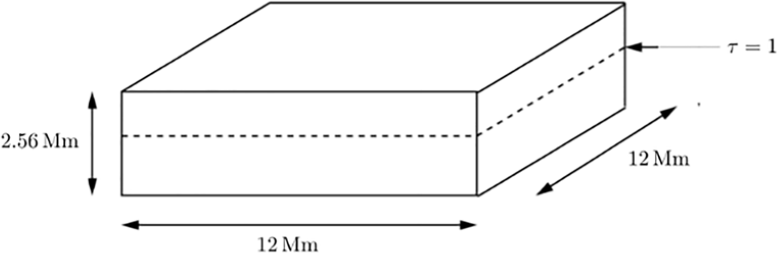
, were generated using the MURaM simulation code Vögler et al. (Reference Vögler, Shelyag, Schüssler, Cattaneo, Emonet and Linde2005) in a domain that includes both the convective zone and the photosphere, as seen in Fig. 1. In this domain, the atmospheric parameters were generated along geometric height. However, since actual inversion methodologies generate the corresponding atmospheric parameters using optical depth as a measurement of height, it is necessary to perform a mapping from geometrical height to optical depth. This process is applied by using the Rosseland opacities Rose (Reference Rose2001), obtaining 21 optical depth values ranging from
 $\log \tau = -2.0$
to
 $\log \tau = 0$
with a sampling of
 $\log \tau = 0.1$
. Apart from the atmospheric parameters, we also have the corresponding spectropolarimetric profiles for each Stokes parameter I, Q, U, and V, which were generated by applying the NLTE numerical code NICOLE (Socas-Navarro et al. Reference Socas-Navarro, de la Cruz Rodríguez, Asensio Ramos, Trujillo Bueno and Ruiz Cobo2015) for 300 wavelength points from
 $6300.5\,\unicode{x212B}$
to
 $6303.5\,\unicode{x212B}$
with a spectral sampling of
 $\Delta \lambda = 0.01\,\unicode{x212B}$
, including the FeI absorption lines in
 $6301.5\,\unicode{x212B}$
and
 $6302.5\,\unicode{x212B}$
. This data was adapted to the Hinode SOT/SP instrument specifications (Tsuneta et al. Reference Tsuneta, Ichimoto, Katsukawa, Nagata, Otsubo, Shimizu, Suematsu, Nakagiri, Noguchi, Tarbell, Title, Shine, Rosenberg, Hoffmann, Jurcevich, Kushner, Levay, Lites, Elmore, Matsushita, Kawaguchi, Saito, Mikami, Hill and Owens2008) by applying the spectral and spatial sampling, the spectral and spatial PSF, and the noise of the instrument, corresponding to gaussian random noise with a
 $\sigma = 5 \times 10^{-3}$
of the continuum intensity
 $I_c$
. Additionally, a weighting was applied to the stokes parameters, realizing that there are differences of orders of magnitude (Lagg et al. Reference Lagg, Solanki, Doerr, Martnez González, Riethmüller, Collados Vera, Schlichenmaier, Orozco Suárez, Franz, Feller, Kuckein, Schmidt, Asensio Ramos, Pastor Yabar, von der Lühe, Denker, Balthasar, Volkmer, Staude, Hofmann, Strassmeier, Kneer, Waldmann, Borrero, Sobotka, Verma, Louis, Rezaei, Soltau, Berkefeld, Sigwarth, Schmidt, Kiess and Nicklas2016; Castellanos Durán et al. Reference Castellanos Durán, Milanovic, Korpi-Lagg, Löptien, van Noort and Solanki2024) between them, which could lead the neural network to prioritize those with higher magnitudes if not treated properly. Also, We applied a filtering technique using the Otsu threshold (Otsu Reference Otsu1979) to separate both regions with high and low intensity, as well as the regions with high and low polarization This approach allows us to have an equal amount of data from both regions, despite their physically different behaviors (Vögler et al. Reference Vögler, Shelyag, Schüssler, Cattaneo, Emonet and Linde2005).
Domain of the MURaM simulated parameters. The domain includes the corrugated surface where the optical depth,
 $\tau$
, meets the condition
 $\log \tau = 1$
, meaning that the domain includes both convective zone and photosphere from the solar atmosphere. The geometrical dimensions of the box are
 $12\,\text{Mm} \times 12\,\text{Mm}$
with a height of
 $2.56\,\text{Mm}$
.

The data extracted correspond to various simulation steps of the MURaM simulation for the quiet sun as observed in the center of the disk. After applying all the preprocessing, we obtained a total of
 $140\,382$
pixels for training. For testing the model on synthetic data, a step of the simulation was left outside the training set.
2.2. Observational
To test the ability of generalization of the neural network model, it is intended to apply it to actual observations. In this case, an observation corresponding to the MODEST catalog (Castellanos Durán et al. Reference Castellanos Durán, Milanovic, Korpi-Lagg, Löptien, van Noort and Solanki2024), with ID 0560, was chosen for testing. This observation corresponds to Active region number 11967 from the NOAA Active Region catalog, observed on February 3, 2014, with a field of view of
 $254'' \times 124''$
, longitude
 $x_c = 16''$
, latitude
 $y_c''=126$
, and heliocentric angle
 $\mu=0.99$
, indicating that we are close to the center of the disk. Additionally, based on this observation, we selected a region that did not include the umbra or penumbra. An image on the continuum of this AR, along with the selected region, is shown in Fig. 2. The atmospheric parameters of this observation in the MODEST catalog correspond to SPINOR 2D spatially coupled inversions (Siu-Tapia et al. Reference Siu-Tapia, Lagg, Solanki, van Noort and Jurčák2017).
Observation with ID 0560 from the MODEST catalog along with the selected region used for testing the neural network model.

3. Neural Network model
3.1. Architecture
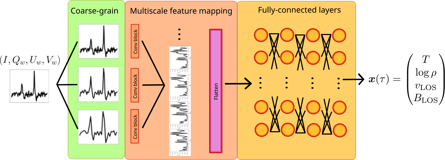
Since the data we are dealing with correspond to spectropolarimetric profiles, it is necessary to use a model that can extract as many features as possible from a 1D signal. For this purpose, we used a mixture of convolutional neural networks (CNNs) with deeply connected layers in an architecture named Multi-Scale Convolutional Neural Network (MSCNN; see Fig. 3), which was first implemented by Jiang et al. (Reference Jiang, He, Yan and Xie2019) with the aim of diagnosing turbine gearbox health through the analysis of the turbine time series. This architecture implements a coarse-grain layer that separates the profiles in different scalings through the application of an average kernel. Each scale passes through a convolutional block that extracts a 1D feature map. All the feature maps are concatenated and then provided to a fully connected block that retrieves the corresponding atmospheric parameters for each analyzed pixel in its outer layer.
Scheme of the MSCNN architecture. The model receives the weighted stokes parameters, coarse-grain and generate feature maps for each scale for finally passing the concatenated maps to a fully connected neural network block that leads to the output of the corresponding atmospheric parameters.

Figure 3 Long description
A diagram of the MSCNN architecture. The model starts with the input of weighted Stokes parameters, represented as four different graphs. These parameters undergo coarse-grain processing, depicted in the green section. The processed data then moves through multiple convolutional blocks, shown in the orange section, generating feature maps at different scales. These feature maps are concatenated and flattened before being passed into a series of fully-connected layers, illustrated in the yellow section. The output of the fully-connected layers provides the corresponding atmospheric parameters, labeled as T, log ρ, v_LOS, and B_LOS.
For training the neural network, an Adam optimizer was used, along with a learning rate of
 $10^{-3}$
and 40 epochs of training.
3.2. Physical constraint
Based on the idea of Physics-Informed Neural Networks (PINNs; Raissi et al. (Reference Raissi, Perdikaris and Karniadakis2019), we modified the loss function to include a term based on the Weak Field Approximation (WFA) for the
 $B_{\text{LOS}}$
. The total loss function uses a weight w to leverage the influence of the terms, where the WFA term is multiplied by w while the mean absolute error (MSE) term is multiplied by
 $1-w$
). The WFA constraint term compares the magnitude approximation for the magnetic field in the line-of-sight with specific optical depth layers that present the most similarity to the results of the
 $B_{\text{LOS}}$
obtained by the WFA. The approximation is only applied under a threshold of WFA
 $B_{\text{LOS}}$
under
 $1000\,$
G and also after the MSE loss term reaches values below
 $4 \times 10^{-4}$
. The values of w used for the experiment were
 $w = 0, 0.001, 0.01, 0.1, 0.5$
.
4. Results
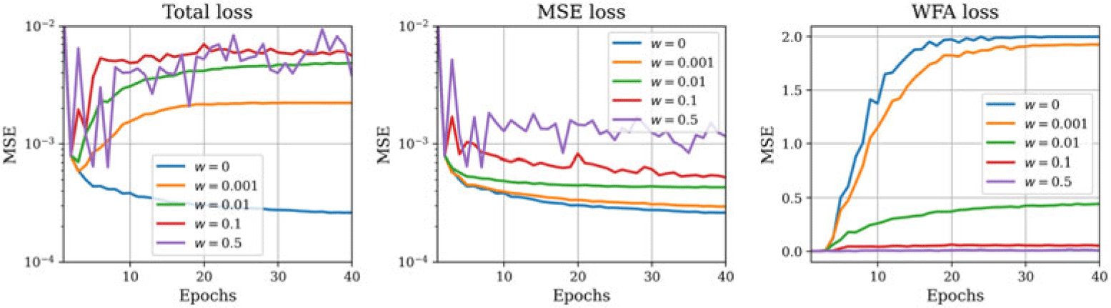
The loss curves for the training process of each of the neural networks for each value of the weight w are shown in Fig. 4. As shown by the curves, the most effective behavior curve that balances the influence of both the typical MSE loss and the WFA term corresponds to the curve of
 $w=0.01$
, which could indicate that the resulting model with this weight value would find a better equilibrium between data information and the physical information of the magnetic field.
Loss curves for each of the values of the weight w that were used. The left hand figure shows the total loss used for applying the backpropagation over the neural network, while the middle and right hand figures correspond to the MSE loss term and WFA loss term, respectively.

The RMSE and correlation values calculated along the optical depth for the MURaM test set compared to the generated data using the MSCNN model are shown in Fig. 5. From these plots, one could infer that, in general, the best RMSE and correlation values along optical depth would correspond to
 $w = 0, 0.01$
, whereas, in some cases,
 $w = 0.01$
seems to outperform the results with no constraint.
RMSE and correlation values calculated along all optical depth nodes comparing the ground-truth MURaM data with the generated one by the neural netwrok after receiving the corresponding stokes profiles for each pixel.

Figure 5 Long description
Panel A: Four scatter plots depict RMSE values for temperature (T), density (log(ρ)), line-of-sight velocity (V_LOS), and line-of-sight magnetic field (B_LOS) against log(τ). Each plot includes multiple data series distinguished by different colors and markers, representing different weighting values (w = 0, w = 0.001, w = 0.01, w = 0.1, w = 0.5). The x-axis is labeled 'log(τ)' and the y-axis is labeled 'RMSE' with appropriate units for each plot. Panel B: Four scatter plots depict Pearson correlation values for the same parameters against log(τ). The x-axis is labeled 'log(τ)' and the y-axis is labeled 'Pearson Correlation'. Each plot includes multiple data series distinguished by different colors and markers, representing different weighting values (w = 0, w = 0.001, w = 0.01, w = 0.1, w = 0.5).
When applied to the observations from the MODEST catalog, Fig. 6 and Fig. 7 show a comparison between the resulting quantities for both weights
 $w = 0, 0.01$
. As can be seen, the MSCNN model with the physical constraint presents results of sharper magnetic fields compared to those of the case without constraint; however, it introduces confusion regarding the direction of the magnetic field flux. Additionally, the RMSE value decreases when the constraint is applied, indicating that the constraint allows for better generalization of the machine learning model when applied to observational data compared to state-of-the-art numerical methods. We only show the resulting magnetic field in the LOS since the thermodynamic quantities and
 $v_{\text{LOS}}$
differ greatly from what is obtained by SPINOR 2D in all cases.
Comparison between the magnetic field in the line-of-sight from the MODEST nodes
 $\log \tau = -0.8, 0$
with the one generated with the MSCNN model with not constraint applied in the loss function.

Comparison between the magnetic field in the line-of-sight from the MODEST nodes
 $\log \tau = -0.8, 0$
with the one generated with the MSCNN model with the constraint applied on the loss function with
 $w = 0.01$

Figure 7 Long description
Panel A: A heat map labeled 'MODST' for log τ = 0. The x and y axes represent spatial coordinates. The color scale ranges from -300 to 300 Gauss, indicating the magnetic field strength in the line-of-sight. Green areas represent positive values, while pink areas represent negative values. Panel B: A heat map labeled 'MSCNN (w=0.01)' for log τ = 0. The x and y axes represent spatial coordinates. The color scale ranges from -300 to 300 Gauss, indicating the magnetic field strength in the line-of-sight. Green areas represent positive values, while pink areas represent negative values. Panel C: A heat map labeled 'MODST' for log τ = -0.8. The x and y axes represent spatial coordinates. The color scale ranges from -300 to 300 Gauss, indicating the magnetic field strength in the line-of-sight. Green areas represent positive values, while pink areas represent negative values. Panel D: A heat map labeled 'MSCNN (w=0.01)' for log τ = -0.8. The x and y axes represent spatial coordinates. The color scale ranges from -300 to 300 Gauss, indicating the magnetic field strength in the line-of-sight. Green areas represent positive values, while pink areas represent negative values.
5. Discussion
According to the results of the model appĺied to the synthetic data for testing, it appears that the model is capable of replicating the atmospheric parameters with remarkable precision and even improving the generation when the WFA constraint is applied. This result replicates when applied to the observational data for the case of the magnetic field in the line-of-sight, noting that when applying the physical constraint, the physical generation of the results compared to those obtained from SPINOR 2D improves. However, it is important to mention that for the remaining parameters, the generalization was not as good, probably indicating that the addition of other constraints is needed.
In general, this work, which is the first in its class on implementing physical constraints based on approximations of the radiative transfer inversion problem as a constraint for applying spectropolarimetric inversions, shows promising results that could motivate the application of physical constraints on data driven models for refining their generalization capabilities. These could also provide hints that an interesting approach for applying machine learning algorithms to analyze solar phenomena might involve supplying information about the physical behavior of the system we are studying to the model in order to achieve improved accuracy.
 τ
 logτ=1
 12Mm×12Mm
 2.56Mm



 logτ=−0.8,0

 logτ=−0.8,0
 w=0.01

 Open access

