
 α





1. Introduction
The Lyman-
 $\alpha$
(Ly
 $\alpha$
) line, corresponding to the
 $2p \rightarrow 1s$
transition of neutral hydrogen, plays a crucial role in interpreting observations and constraining galaxy formation physics in the high-redshift Universe (Partridge & Peebles Reference Partridge and Peebles1967). As hydrogen becomes ionised in H ii regions around young stars, recombination leads to efficient emission of Ly
 $\alpha$
radiation. Subsequently, Ly
 $\alpha$
photons undergo a resonant scattering process in the neutral hydrogen surrounding compact ionised bubbles where absorption into the 2p state is almost immediately followed by re-emission back into the 1s state. This resonant scattering process makes Ly
 $\alpha$
radiative transfer conceptually and numerically complex, especially in realistic environments with extremely high optical depth (Dijkstra Reference Dijkstra2014). When benchmarking Ly
 $\alpha$
radiation pressure calculations, it becomes apparent that frequencies around line centre are particularly problematic, highlighting the need to understand its behaviour in greater detail. The purpose of this paper is therefore to analyse and decompose the frequency-dependent properties of Ly
 $\alpha$
radiative transfer to better assess the accuracy and limitations of analytical methods adopting diffusion approximations compared to numerical numerical simulations.
Foundational works motivated the study of Ly
 $\alpha$
radiative transfer from back-of-envelope scaling arguments, providing physical insights into resonant scattering with significant differences from the properties of monochromatic transfer (Osterbrock Reference Osterbrock1962; Adams Reference Adams1972, Reference Adams1975; Hansen & Oh Reference Hansen and Oh2006). Analytical methods have been developed over time, which are mainly based on a diffusion approximation in the full radiative transfer equation for partial frequency redistribution (Unno Reference Unno1952; Hummer Reference Hummer1962) rigorously understood within a Fokker–Planck framework (Rybicki & Dell’Antonio Reference Rybicki and Dell’Antonio1994; Meiksin Reference Meiksin2006). The first accurate solutions were for the idealised cases of uniform slab, spherical, and cube geometries (Harrington Reference Harrington1973; Neufeld Reference Neufeld1990; Dijkstra et al. Reference Dijkstra, Haiman and Spaans2006; Tasitsiomi Reference Tasitsiomi2006b), as well as extended Ly
 $\alpha$
halos in an expanding neutral intergalactic medium (Loeb & Rybicki Reference Loeb and Rybicki1999). Further generalisations have recently been made, such as analysing the Wouthuysen-Field effect (Higgins & Meiksin Reference Higgins and Meiksin2012; Seon & Kim Reference Seon and Kim2020), improvements for boundary conditions and time dependence (McClellan et al. Reference McClellan, Davis and Arras2022), Ly
 $\alpha$
feedback during direct collapse black hole formation (Ge & Wise Reference Ge and Wise2017; Smith et al. Reference Smith, Becerra, Bromm and Hernquist2017b), methods for Ly
 $\alpha$
radiation hydrodynamics (Smith et al. Reference Smith, Bromm and Loeb2017a, Reference Smith, Tsang, Bromm and Milosavljević2018; Kimm et al. Reference Kimm, Haehnelt, Blaizot, Katz, Michel-Dansac, Garel, Rosdahl and Teyssier2018; Mushano et al. Reference Mushano, Ogawa, Ohsuga, Yajima and Omukai2024; Nebrin et al. Reference Nebrin, Smith, Mellema, Lorinc and Manzoni2026), and the studies that motivate this paper, exploring emissivity, density, destruction, and velocity gradients (Lao & Smith Reference Lao and Smith2020; Nebrin et al. Reference Nebrin, Smith, Lorinc, Hörnquist, Larson, Mellema and Giri2025; Smith et al. Reference Smith, Lorinc, Nebrin and Lao2025).
These theoretical developments are central to understanding a wide array of physical applications at Cosmic Dawn where Ly
 $\alpha$
feedback may act as a primary driver of pre-supernova stellar feedback. These include regulating the star formation efficiency and shaping the initial mass function of Population III stars (Wise et al. Reference Wise, Abel, Turk, Norman and Smith2012; Nebrin Reference Nebrin2022; Klessen & Glover Reference Klessen and Glover2023), destroying natal gas clouds during the formation of metal-poor star clusters and ultra-faint dwarf galaxies (Abe & Yajima Reference Abe and Yajima2018), and providing a critical source of internal radiation pressure capable of impeding super-Eddington accretion onto early massive black holes (Inayoshi et al. Reference Inayoshi, Visbal and Haiman2020; Mushano et al. Reference Mushano, Ogawa, Ohsuga, Yajima and Omukai2024). Additionally, capturing these precise force updates is essential for calibrating subgrid prescriptions in large-scale cosmological galaxy formation simulations that currently omit this process entirely Nebrin et al. (Reference Nebrin, Smith, Mellema, Lorinc and Manzoni2026).
With the aid of high-performance computing, direct numerical solutions to the radiative transfer equation typically employ Monte Carlo radiative transfer (MCRT), which can be compared with these analytical results for validation before generalising to more complex geometries (Zheng & Miralda-Escudé Reference Zheng and Miralda-Escudé2002; Dijkstra et al. Reference Dijkstra, Haiman and Spaans2006; Tasitsiomi Reference Tasitsiomi2006a; Verhamme et al. Reference Verhamme, Schaerer and Maselli2006; Semelin et al. Reference Semelin, Combes and Baek2007; Laursen et al. Reference Laursen, Razoumov and Sommer-Larsen2009; Yajima et al. Reference Yajima, Li, Zhu and Abel2012; Smith et al. Reference Smith, Safranek-Shrader, Bromm and Milosavljević2015; Gronke & Dijkstra Reference Gronke and Dijkstra2016; Michel-Dansac et al. Reference Michel-Dansac, Blaizot, Garel, Verhamme, Kimm and Trebitsch2020; Seon & Kim Reference Seon and Kim2020; Byrohl & Nelson Reference Byrohl and Nelson2025). Most MCRT methods rely on core-skipping algorithms to significantly reduce the computational load of repeated core scatterings, which preserves the emergent spectra but can introduce errors for the internal radiation field. Recently, the dynamical impact of Ly
 $\alpha$
, arising from the momentum transfer that occurs at each scattering event, has been explored as a potentially dominant form of early (i.e. pre-supernova) stellar feedback, especially relevant in the dust-poor conditions of early galaxies (Dijkstra & Loeb Reference Dijkstra and Loeb2008; Smith et al. Reference Smith, Bromm and Loeb2016, Reference Smith, Bromm and Loeb2017a; Abe & Yajima Reference Abe and Yajima2018; Kimm et al. Reference Kimm, Haehnelt, Blaizot, Katz, Michel-Dansac, Garel, Rosdahl and Teyssier2018; Tomaselli & Ferrara Reference Tomaselli and Ferrara2021; Mushano et al. Reference Mushano, Ogawa, Ohsuga, Yajima and Omukai2024; Nebrin et al. Reference Nebrin, Smith, Lorinc, Hörnquist, Larson, Mellema and Giri2025; Ferrara et al. Reference Ferrara, Manzoni and Ntormousi2025; Manzoni & Ferrara Reference Manzoni and Ferrara2025). To this end, accurate force calculations are crucial in determining the true dynamical impact of Ly
 $\alpha$
radiation pressure in such environments.
MCRT provides the gold standard for numerical Ly
 $\alpha$
radiation transport, since it solves the full radiative transfer equation without any approximations while remaining straightforward to understand and generalise. The MCRT framework makes it possible to track the internal radiation field (e.g. number of scatterings, energy density, momentum exchange, and pressure) and externally observed quantities (e.g. escape fractions, spectral flux, and surface brightness). For internal properties, various biasing techniques can be employed to increase the speed of statistical convergence. The most important ones include differentiating between an event-based sampling approach where photons are treated individually and path-based approaches where photons packets have an associated weight that is updated based on path lengths traversed and the probability of events occurring along the trajectory (Lucy Reference Lucy1999; Smith et al. Reference Smith, Kannan, Tsang, Vogelsberger and Pakmor2020). For properties that are sensitive to the details of scattering, such as the force, an event-based approach can significantly outperform a path-based one, but other properties, such as energy density and dust absorption, greatly benefit from the implicit treatment of changes during transport, so a path-based approach is better. However, even with statistical biasing techniques, MCRT can exhibit poor convergence properties, especially as the optical depth increases, which leads to the need to sample a large number of photon paths before solutions can be fully trusted (Camps & Baes Reference Camps and Baes2018). The convergence properties of resonant-line MCRT is further complicated by the frequency-dependent opacity (Kasiri et al. Reference Kasiri, Smith, Lorinc, Nebrin and Kimura2026).
The extreme line-centre optical depths make resonant-line Ly
 $\alpha$
MCRT a computationally expensive method, which led to the development of various acceleration techniques. One of the most common and highly beneficial schemes involves core-skipping algorithms, which preferentially choose the velocity of the scattering atom to push core photons, which are trapped due to extreme optical depths (
 $\tau_0 \sim 10^6$
–
 $10^{10}$
), out into the wing where they can continue their frequency diffusion process (Ahn et al. Reference Ahn, Lee and Lee2002; Smith et al. Reference Smith, Safranek-Shrader, Bromm and Milosavljević2015; Michel-Dansac et al. Reference Michel-Dansac, Blaizot, Garel, Verhamme, Kimm and Trebitsch2020). The speedups can be as large as
 $\sim$
 $10^3$
times faster, which makes the use of such methods appealing. Alternative speedups can be achieved by resonant Discrete Diffusion Monte Carlo (rDDMC) methods by sacrificing the tracking of exact photon trajectories (Smith et al. Reference Smith, Tsang, Bromm and Milosavljević2018). Although external field properties are not significantly affected by the use of acceleration techniques, core skipping can introduce errors in the internal radiation field, especially properties that are sensitive to the total number of scatterings. This means that using any amount of core skipping leads to errors in force calculations, even when the MCRT simulation statistics are fully converged.
As the dynamical importance of Ly
 $\alpha$
feedback receives additional attention, it is necessary to devise methods where force calculations remain accurate. Fortunately, recent analytical progress in Ly
 $\alpha$
radiative transfer allows for the stratified development of such methods (Lao & Smith Reference Lao and Smith2020; Tomaselli & Ferrara Reference Tomaselli and Ferrara2021; McClellan et al. Reference McClellan, Davis and Arras2022; Nebrin et al. Reference Nebrin, Smith, Lorinc, Hörnquist, Larson, Mellema and Giri2025; Smith et al. Reference Smith, Lorinc, Nebrin and Lao2025). In this paper, we extend these results by deriving the spectral distributions of the force multiplier
 $M_{\text{F}}$
and the photon trapping time
 $t_{\text{trap}}$
(related to the energy density) for idealised clouds containing neutral hydrogen. We then compare this with the results of MCRT simulations that do not adopt core skipping. This is a robust test of the applicability of the diffusion approximation across the entire spatial–spectral domain of resonant-line transfer. We further explore numerous related numerical experiments to probe how Ly
 $\alpha$
photons scatter and escape optically-thick environments.
This paper is organised as follows. In Section 2, we review the fundamentals of Ly
 $\alpha$
radiative transfer relevant for this paper, including the MCRT algorithm. In Section 3 we derive spectral distributions for the force multiplier, the trapping time, and the number of scatterings. We gain insight into the various diffusion approximations, specifically the breakdown of the Fokker–Planck approximation in the core. We introduce a modification to the MCRT algorithms based on the gradient of the energy density to increase the convergence rate of force calculations when core skipping is not used and note that the analytical solution can be used as minor, yet incomplete, correction to the force multiplier when core skipping is used. Finally, we find that the Eddington approximation does not hold everywhere within the cloud, especially near the core–wing transition. In Section 4, we provide insight into resonant line radiative transfer from robust high-optical depth MCRT simulations with no core skipping, such as the average radius reached and path length traversed before reaching a given frequency for the first time, and we also show the fraction that escapes a certain frequency and compare with the integrated emergent spectra. In Section 5, we show properties of RT that show anomalous diffusion in fat-tailed distributions along with some statistics about excursions that lead to escape and the probability that a photon at a given frequency returns to the core. In Section 6, we present a summary of our findings and discuss the consequences for numerical algorithms.
2. Ly
 $\boldsymbol{\alpha}$
radiative transfer

In this section, we provide some background on Ly
 $\alpha$
radiative transfer, focusing on aspects relevant for MCRT simulations and the theoretical aspects necessary to calculate properties internal to the cloud. During transport, photons probabilistically interact with neutral hydrogen intervening in its path, with a frequency-dependent mean-free path of
 $\lambda_{\text{mfp}}(\nu) = 1/$
n
H i
 $\sigma_\nu$
, where n
H i
is the number density of neutral hydrogen (which we assume is uniform in this paper) and
 $\sigma_\nu$
is the frequency-dependent cross section. As photons undergo multiple scatterings, they randomly walk in both space and frequency, where the path lengths between scatterings depend on the frequency. To fully describe the steady-state radiation field we need to know the specific intensity
 $I_\nu({\boldsymbol{{r}}},{\boldsymbol{{n}}})$
, which is the energy per unit frequency,
 $\nu$
, and the direction of propagation
 ${\boldsymbol{{n}}}$
, as a function of spatial position
 ${\boldsymbol{{r}}}$
. For a static medium with no dust, the steady-state radiative transfer equation is
 \begin{equation} {\boldsymbol{{n}}} \boldsymbol{\cdot} \boldsymbol{\nabla} I_\nu = j_\nu - k_\nu I_\nu + \iint k_{\nu'} I_{\nu'} R_{\nu', {\boldsymbol{{n}}}' \rightarrow \nu, {\boldsymbol{{n}}}} \, \text{d}\Omega' \text{d}\nu' \, ,\end{equation}
where
 $j_\nu$
and
 $k_\nu$
are the emission and absorption coefficients, respectively. The integral in the last term on the right accounts for the frequency redistribution caused by partially coherent scattering (e.g. Dijkstra Reference Dijkstra2014). The conditional redistribution function
 $R_{\nu', {\boldsymbol{{n}}}' \rightarrow \nu, {\boldsymbol{{n}}}}$
is the differential probability per unit initial photon frequency
 $\nu'$
and per unit initial directional solid angle
 $\Omega'$
that scattering of such a photon travelling in the direction
 ${\boldsymbol{{n}}}'$
would place the scattered photon at frequency
 $\nu$
and in the direction of the unit vector
 ${\boldsymbol{{n}}}$
. The development of resonant scattering redistribution functions is given in detail in Hummer (Reference Hummer1962) and Hubeny & Mihalas (Reference Hubeny and Mihalas2015). For Ly
 $\alpha$
the appropriate redistribution function is
 $R_{\text{II}}$
, but notice the way we define it here that it is a conditional probability rather than a joint probability. This makes for easier analytical progress. In treating single-line problems like Ly
 $\alpha$
, it is convenient to switch to the dimensionless frequency
 \begin{equation} x \equiv \frac{\nu - \nu_0}{\Delta \nu_{\text{D}}} \, ,\end{equation}
where
 $\nu_0 = 2.466 \times 10^{15} \, \text{Hz}$
is the frequency at line centre,
 $\Delta \nu_{\text{D}} \equiv (v_{\text{th}}/c)\nu_0$
the Doppler width of the profile, and
 $v_{\text{th}} \equiv (2 k_{\text{B}} T / m_{\text{H}})^{1/2}$
the thermal velocity. To characterise the frequency dependence on the cross section, we define the Hjerting–Voigt function
 $H(a,x) = \sqrt{\pi} \Delta \nu_{\text{D}} \phi_{\text{Voigt}}(a, \nu)$
as the dimensionless convolution of Lorentzian and Maxwellian distributions,
 \begin{equation} H(a,x) = \frac{a}{\pi} \int_{-\infty}^\infty \frac{e^{-y^2}\text{d}y}{a^2+(y-x)^2} \approx \begin{cases} e^{-x^2} & \quad \text{`core'} \\ {\displaystyle \frac{a}{\sqrt{\pi} x^2} } & \quad \text{`wing'} \end{cases} \, .\end{equation}
The ‘damping parameter’,
 $a \equiv \Delta \nu_\mathrm{L} /2 \Delta \nu_\mathrm{D}$
, describes the relative thermal broadening compared to the natural line width. We focus on the case of Ly
 $\alpha$
where
 $\Delta \nu_{\text{L}} = 9.936 \times 10^7 \, \text{Hz}$
, and, in an isothermal gas, the damping parameter traces the temperature T. Specifically
 $a \approx 4.702 \times 10^{-4} \, (T/10^4 \, \text{K})^{-1/2}$
. The cross section at dimensionless frequency x is
 $\sigma_x = \sigma_0 H(a,x)$
, where
 $\sigma_0 = 5.898 \times 10^{-14} \, (T/10^4 \, \text{K})^{-1/2} \, \mathrm{cm}^2$
is the cross section at line centre. This allows us to give the optical depth as
 \begin{equation} \tau_x = \int_{\text{path}} k({\boldsymbol{{r}}}) \, H(a,x) \, \text{d}\ell \, ,\end{equation}
where
 $k({\boldsymbol{{r}}}) =$
n
H i
 $({\boldsymbol{{r}}}) \sigma_0$
is the absorption coefficient at line centre at position
 ${\boldsymbol{{r}}} = {\boldsymbol{{r}}}_0 + \ell {\boldsymbol{{n}}}$
. We define the line centre optical depth
 $\tau_0$
as the integrated value from the centre to the outer boundary of a spherical cloud, and use this throughout as a simulation parameter.
In general, it is only possible to solve Eq. (1) numerically, however further analytical progress can be made if the product
 $a \tau_0$
is sufficiently large (for a comprehensive discussion see Nebrin et al. Reference Nebrin, Smith, Lorinc, Hörnquist, Larson, Mellema and Giri2025). In this regime, scattering may be treated as a diffusion process in both space and frequency, and we find analytical solutions for the angular-averaged frequency
 $J_x \equiv \frac{1}{4\pi} \int I_x \, \text{d} \Omega$
. To do so, we integrate Eq. (1) further defining
 ${\boldsymbol{{H}}}_x \equiv \frac{1}{4\pi} \int {\boldsymbol{{n}}} I_x \, \text{d} \Omega$
to give us
 \begin{align} \ \boldsymbol{\nabla} \boldsymbol{\cdot} {\boldsymbol{{H}}}_x = \int \frac{j_x}{4\pi} \, \text{d} \Omega - k_x J_x + \int k_{x'} J_{x'} R_{x' \rightarrow x} \, \text{d}x' \, ,\end{align}
where
 $R_{x' \rightarrow x} \equiv (4\pi)^{-2} \iint \text{d}\Omega' \text{d}\Omega \, R_{x', {\boldsymbol{{n}}}' \rightarrow x, {\boldsymbol{{n}}}}$
is the angular-averaged redistribution function, with
 $R_{x' \rightarrow x} = \Delta\nu_{\text{D}}^2 \, R_{\nu' \rightarrow \nu}$
, and
 $J_x = \Delta\nu_{\text{D}} J_\nu$
. In optically thick environments, the intensity is nearly isotropic (Eddington approximation), and we can apply Fick’s law as a closure relation to the moment equations:
 \begin{equation} {\boldsymbol{{H}}}_x \approx -\frac{\boldsymbol{\nabla} J_x}{3 k_x} \, .\end{equation}
The Fokker–Planck approximation (FPA) is often used to approximate the redistribution integral, but, as will be explained below, the common form of the approximation is only accurate for wing frequencies (Rybicki & Dell’Antonio Reference Rybicki and Dell’Antonio1994; Rybicki Reference Rybicki2006; McClellan et al. Reference McClellan, Davis and Arras2022) where frequency diffusion occurs. The error of the FPA is explicitly shown in the Appendix A from which it is clear that the Fokker–Planck treatment can only be expected to have good results in the wing. The usual approximation is
 \begin{align} -k_xJ_x + &\int k_{x'} J_{x'} R_{x' \rightarrow x} \, \text{d}x' \approx \frac{1}{2}\frac{\partial}{\partial x}\left(k_x\frac{\partial J_x}{\partial x}\right) \, ,\end{align}
from which one can write down the diffusion equation under an analytical transform and solve for J. Then one can derive the radiation energy density, related to the angular-averaged intensity as
 $u({\boldsymbol{{r}}}) = \frac{4\pi}{c} \int J_x({\boldsymbol{{r}}})\,\text{d}x$
, the trapping time, defined as
 $t_{\text{trap}} \equiv \mathcal{L}^{\, -1} \int u({\boldsymbol{{r}}})\,\text{d}V$
with
 $\mathcal{L}$
the source luminosity,Footnote
a
and the outward force multiplier
 \begin{equation} M_{\text{F}} \equiv \mathcal{L}^{\, -1} \iint k({\boldsymbol{{r}}}) F \,\text{d}x\,\text{d}V \approx -\frac{c}{3\mathcal{L}} \int \nabla u({\boldsymbol{{r}}})\,\text{d}V \, ,\end{equation}
where the second expression follows from Ficks law, replacing the flux by
 $F \approx -c \nabla u / 3k$
for diffusive radiation. The force multiplier quantifies the enhancement of the momentum coupling compared to the single scattering limit of
 $\mathcal{L}/c$
(e.g. Dijkstra & Loeb Reference Dijkstra and Loeb2008). We define the Ly
 $\alpha$
scattering rate as
 $P_\alpha = (4\pi / \mathcal{L})\int \sigma_x J_x \, \text{d} x$
, where we normalise by the total luminosity
 $\mathcal{L}$
since we express intensity in terms of energy instead of photon number, as previous authors have done in Higgins & Meiksin (Reference Higgins and Meiksin2012) and Seon & Kim (Reference Seon and Kim2020). Then the average number of scatterings is
 $N_{\text{scat}} = \int P_\alpha$
n
H i
 $\,\text{d} V$
which becomes
 \begin{equation} N_{\text{scat}} = \frac{4 \pi}{\mathcal{L}} \iint k({\boldsymbol{{r}}})\,H(a,x)\,J_x({\boldsymbol{{r}}})\,\text{d} x\,\text{d} V \, .\end{equation}
The diffusion approximation has been analytically explored in numerous works (e.g. Harrington Reference Harrington1973; Neufeld Reference Neufeld1990; Dijkstra et al. Reference Dijkstra, Haiman and Spaans2006; Tomaselli & Ferrara Reference Tomaselli and Ferrara2021; McClellan et al. Reference McClellan, Davis and Arras2022), however, the notation and definitions in this paper are consistent with Lao & Smith (Reference Lao and Smith2020) and Smith et al. (Reference Smith, Lorinc, Nebrin and Lao2025), which explore more general solutions that account for gradient structures in density and velocity space, respectively. In Nebrin et al. (Reference Nebrin, Smith, Lorinc, Hörnquist, Larson, Mellema and Giri2025), a combination of a wide range of effects were analytically treated. All analytical results were validated with MCRT simulations, and the diffusion approximation is accurate as long as
 $a\tau_0 \gg 1\,000$
.
To directly solve Eq. (1) without any approximations, we employ the MCRT algorithm which samples a large number of individual photon paths to generate statistically converged properties of the radiation field. We utilise the Cosmic Ly
 $\alpha$
Radiative Transfer code (colt), which is described in Smith et al. (Reference Smith, Safranek-Shrader, Bromm and Milosavljević2015, Reference Smith, Ma, Bromm, Finkelstein, Hopkins, Faucher-Giguère and Kereš2019, Reference Smith2022) and McClymont et al. (Reference McClymont, Smith and Tacchella2025). Concisely, the optical depth to be traversed between scattering events is drawn from an exponential distribution, consistent with the interpretation of the optical depth
 $\tau_x$
from Eq. (4) as the inverse mean free path between photon interactions. Once the photon has traversed enough distance to attenuate this randomly drawn optical depth, the photon undergoes a scattering event, and the frequency and direction are updated accordingly. This process is repeated until the photon escapes the computational domain. Sampling enough photon paths will result in converged properties of the radiation field thus solving Eq. (1) for the intensity
 $I({\boldsymbol{{r}}},x,{\boldsymbol{{n}}})$
and related quantities with the definitions provided.
Although accurate when fully converged without using any acceleration scheme, resonant-line MCRT suffers significantly from repeated core scatterings when the photon is near the line centre frequency, which causes the algorithm to slow down. Each time the photon goes to a resonant frequency, it gets trapped in space until a random excursion into the wing of the line (caused by an interaction with a hydrogen atom of sufficiently large velocity) enables the photon to move a non-negligible distance. Further, the error scales linearly with optical depth, meaning that higher-density simulations would require more photons for the same level of error, contributing to a very long runtime to produce converged simulations. The exact details of Ly
 $\alpha$
MCRT convergence are given in Kasiri et al. (Reference Kasiri, Smith, Lorinc, Nebrin and Kimura2026). To avoid photon trapping, the core-skipping algorithm picks an interaction with an atom that has enough velocity to push the core photons out into the wing of the line, the boundary of which will be defined in Section 3. Core-skipping retains accuracy for emergent properties, since photons cannot move in physical space until they diffuse in frequency and are already in the wing. Unfortunately, core photons can considerably impact internal properties, specifically the force multiplier, since repeated core scatterings impart momentum in a way that does not cancel out. Clearly, the inherent accuracy of Monte Carlo is challenged by core-skipping, especially for frequency-dependent quantities, which we explore in this paper as the cause for missing momentum when comparing analytical results to Monte Carlo results. To avoid misinterpreting MCRT simulations, we refrain from using core-skipping in our simulations unless otherwise mentioned.
3. Spectral distributions of radiation
Core photons can contribute significantly to internal radiation properties, such as the total number of scatterings, the trapping time, and the total momentum imparted. Fully capturing these contributions in simulations requires running MCRT simulations without the commonly adapted core-skipping algorithms that result in a significant ray-tracing speed-up. From previous analytical developments in Ly
 $\alpha$
RT (Lao & Smith Reference Lao and Smith2020; Nebrin et al. Reference Nebrin, Smith, Lorinc, Hörnquist, Larson, Mellema and Giri2025; Smith et al. Reference Smith, Lorinc, Nebrin and Lao2025), we can derive spectral distributions of internal fields to quantify the relative contribution of core scatterings relative to wing scatterings based on the diffusion approximation for the various internal quantities. We use the results from Lao & Smith (Reference Lao and Smith2020) in reference to spherical geometry without any velocity or density gradients. We compare these distributions with MCRT simulations that do not use core-skipping to analyse the accuracy of our analytical findings. Using core-skipping gives results that converge to the wrong answer because of the missing core contributions. To amend this, a semi-analytical core correction can approximate core contributions to the force multiplier, trapping time, and number of scatterings while allowing for the use of core skipping. This works quite well for the trapping time and the number of scatterings, but the force multiplier suffers from the breakdown of diffusion approximations, which we elaborate on. More practically, we show that the force can be efficiently calculated from a quickly convergent energy density or pressure calculation with even less error than the analytical correction. We compare this with an upcoming Ly
 $\alpha$
code based on the diffusion approximation, lydion (Nebrin et al. Reference Nebrin, Smith, Mellema, Lorinc and Manzoni2026). Future calculations rely heavily on
 $\tilde{x}$
, defined in differential form as
 \begin{equation} \text{d}\tilde{x} = \sqrt{\frac{2}{3}}\frac{\text{d}x}{\tau_0 H(a, x)} \, .\end{equation}
Here
 $\tilde{x}$
depends on both the temperature and frequency through H(a, x). When finding exact solutions, we use numerical integration to solve for
 $\tilde{x}(x)$
. To distinguish between the ‘core’ and ‘wing’ frequencies, we use the approximations in Eq. (3) to find
 \begin{equation} \text{Wing: }\, \tilde{x} \approx \sqrt{\frac{2\pi}{27}} \frac{x^3}{a \tau_0} \quad \text{Core: } \,\tilde{x} \approx \sqrt{\frac{\pi}{6}} \frac{\text{erfi}(x)}{\tau_0} \,,\end{equation}
where the imaginary error function is
 $\text{erfi}(x) = -i\,\text{erf}(i x)$
. Equating the two approximations and solving gives a critical frequency
 ${x_{\text{cw}}^\ast}$
. This frequency is different from
 $x_{\text{cw}}$
from Eq. (21) of Smith et al. (Reference Smith, Safranek-Shrader, Bromm and Milosavljević2015), which is defined by equating the two approximations in Eq. (3) for H(a, x). We show
 $x_{\text{cw}}^\ast$
, defined by equating the approximations after integrating
 $1/H(a,x)$
, better characterises differences in behaviour between the core and the wing than the traditional
 $x_{\text{cw}}$
. The transcendental equation for
 $x_{\text{cw}}^\ast$
is
 \begin{equation} \frac{2}{3} {x_{\text{cw}}^\ast}^3 = a \,\text{erfi}({x_{\text{cw}}^\ast}) \, ,\end{equation}
and an accurate fitting formula in our relevant parameter range is
 \begin{equation} {x_{\text{cw}}^\ast}(a) = \frac{1.53760 - 0.37024 \ln(a)}{0.85538 - 0.04730 \ln(a)} \, .\end{equation}
We plot the relative error, which is strongly bounded over the relevant parameter range, in Figure 1 and show the exact form in an inset versus the fitting formula along with the value of
 $x_{\text{cw}}$
as a reference in red to highlight the difference in definition. The procedure through this section is as follows: let Q be a general radiative transfer quantity, for example, from Eqs. (8)–(9). We define the spectral distribution of Q as the frequency derivative
 $\text{d} Q/\text{d} x \equiv Q_x$
. Similarly, the contribution to Q over a frequency range
 $x_{\text{min}}$
to
 $x_{\text{max}}$
is
 $\int_{x_{\text{min}}}^{x_{\text{max}}} Q_x \text{d} x$
. To find the core contribution,
 $Q^{\text{core}}$
, take
 $x_{\text{max}} = x_{\text{cw}}^\ast$
and
 $x_{\text{min}} = - x_{\text{cw}}^\ast$
. Then the wing contribution is defined as
 $Q^{\text{wing}} \equiv Q - Q^{\text{core}}$
. The fraction of contribution to Q coming from frequencies
 $\lt|x|$
is defined as
 \begin{equation} f_{Q,\lt|x|} \equiv \frac{\int_{-x}^x Q_x \,\text{d} x}{\int_{-\infty}^{\infty} Q_x \,\text{d} x} \, ,\end{equation}
and the label can vary depending on Q, but is descriptive of the quantity.
The relative percent error in the fitting formula given by Eq. (13) is shown in green. The bound on the error is very low for the parameter range of interest. In the inset plot, the exact solution for largest solution to Eq. (12) found with a root finder is shown in black while the red line indicates
 $x_{\text{cw}}$
defined as the frequency where H(a, x) transitions from a Gaussian to a Lorentzian distribution, which is important for core-skipping algorithms.

3.1. Spectral trapping time
The spectral trapping time in a general finite-cloud geometry is defined as
 \begin{equation} t_{\text{trap},x} = \frac{\text{d} t_{\text{trap}}}{\text{d} x} \equiv \frac{4 \pi}{\mathcal{L} c} \int J_x({\boldsymbol{{r}}}) \,\text{d} V \, .\end{equation}
We define volume-weighted averages as
 \begin{equation} \langle {\, f} \rangle \equiv \frac{\int f({\boldsymbol{{r}}})\,\text{d}V}{\int \text{d}V} \, .\end{equation}
In spherical geometry, with a total cloud radius R we have
 $t_{\text{trap},x}/t_{\text{light}} = (16 \pi^2 R^2 / 3\mathcal{L})\,\langle J_x \rangle$
, where
 $\langle J_x \rangle$
is the average internal spectrum at a given frequency x, and the light crossing time is
 $t_{\text{light}} \equiv R/c$
. For a static uniform density spherical point source cloud this simplifies to (see Eq. 90 in Lao & Smith Reference Lao and Smith2020)
 \begin{equation} \frac{t_{\text{trap},x}}{t_{\text{light}}} = \frac{\sqrt6}{\pi} \ln\left(1 + e^{-\pi |\tilde{x}|}\right) \, .\end{equation}
To find the trapping time contributions from various frequency ranges, we must integrate the spectral trapping time over a frequency range. We consider the two cases by defining the core contribution as the quantity integrated over core frequencies (
 $|x| \leq x_{\text{cw}}^\ast$
), and the wing contribution as the quantity integrated over wing frequencies (
 $|x| \gt x_{\text{cw}}^\ast$
). Under the core approximation,
 \begin{align} t_{\text{trap},x}^{\text{core}}\,/\,t_{\text{light}} &= \frac{\sqrt6}{\pi} \ln\left[1 + \exp\left(-\sqrt{\frac{\pi^3}{6}} \frac{\text{erfi}(|x|)}{\tau_0}\right)\right] \notag \\ &\approx \frac{\sqrt6}{\pi} \ln(2) \approx 0.540 \, ,\end{align}
where we make use of the fact that
 $x \lt {x_{\text{cw}}^\ast} \implies \text{erfi}(x)/\tau_0 \ll 1$
for any physical optical depth under the diffusion regime. Thus, after integrating from
 $-{x_{\text{cw}}^\ast}$
to
 ${x_{\text{cw}}^\ast}$
, we find
 $t_{\text{trap}}^{\text{core}} \,/\, t_{\text{light}} = (2\sqrt{6}/\pi \,\ln(2)) \, {x_{\text{cw}}^\ast}$
, which only varies weakly with temperature. Under the wing approximation,
 \begin{equation} t_{\text{trap},x}^{\text{wing}}\,/\,t_{\text{light}} = \frac{\sqrt6}{\pi} \ln\left[1 + \exp\left(-\sqrt{\frac{2\pi^3}{27}} \frac{|x^3|}{a\tau_0}\right)\right] \, ,\end{equation}
which may be asymptotically expanded to get a far wing approximation but needs to be numerically integrated to find the general wing contribution. In the limit as
 $x \rightarrow 0$
, both the core and wing approximation approach the same value, so the overall spectral distribution of the trapping time is well described by the wing approximation for all frequencies while the core contribution quickly dies off for
 $|x| \gt {x_{\text{cw}}^\ast}$
. In the bottom panel of Figure 2, we show the spectral trapping time from Eq. (17) with thin lines, and MCRT results with thick lines. In the top panel of Figure 2, we integrate the spectral distribution giving the contribution from the trapping time coming from frequencies
 $\lt|x|$
. The agreement is excellent and the error decreases as
 $\tau_0$
increases. As expected, the distribution in the core is roughly constant at all optical depths, and the wing spread increases as the optical depth increases, which leads to a broader emission line. This follows from increased diffusion as the medium becomes more opaque for wing photons. The wing contribution quickly beats out the core contribution as
 $\tau_0$
increases.
A comparison between analytical trapping time (thin lines) and MCRT simulations (thick lines) as defined in Eq. (15). Bottom Panel: The analytical
 $t_{\text{trap},x}$
from Eq. (17) evaluated exactly with numerical integration for various values of
 $\tau_0$
with a fixed temperature of
 $T = 10^4 \,\text{K}$
compared with binned contributions from MCRT simulations. The vertical line shows
 $x_{\text{cw}}^\ast$
at this temperature. Top Panel: The cumulative fraction of
 $t_{\text{trap}}$
from frequencies
 $\lt |x|$
(
 $f_{\text{trap}}$
) as defined in Eq. (14). The agreement here is almost perfect once the diffusion approximation is valid.

3.2. Spectral number of scatterings
A comparison between the analytical spectral number of scatterings (thin lines) and MCRT simulations (thick lines) as defined in Eq. (20). Bottom Panel: The analytical
 $N_{\text{scat},x}$
from Eq. (21) normalised by
 $\tau_0$
as a function of x at various
 $\tau_0$
at a fixed temperature
 $T = 10^4 \, \text{K}$
compared to binned MCRT simulation data. The vertical dotted line shows the value of
 $x_{\text{cw}}^\ast$
for this temperature. Top Panel: The cumulative scattering fraction
 $f_{\text{scat},\lt|x|}$
as defined in Eq. (14).

Figure 3. Long description
Panel A: A line graph showing the cumulative scattering fraction as a function of x. The horizontal axis is labeled x and ranges from 0.1 to 100. The vertical axis is labeled f scatter subscript x and ranges from 0 to 1. The graph includes multiple lines representing different values of tau subscript 0, with labels in different colors: red for tau subscript 0 equals 10 to the power of 6, purple for tau subscript 0 equals 10 to the power of 7, blue for tau subscript 0 equals 10 to the power of 8, cyan for tau subscript 0 equals 10 to the power of 9, and green for tau subscript 0 equals 10 to the power of 10. The lines show an increasing trend. Panel B: A line graph showing the logarithm of the number of scatterings normalized by tau subscript 0 as a function of x. The horizontal axis is labeled x and ranges from 0.1 to 100. The vertical axis is labeled log subscript 10 of N scatter subscript x divided by tau subscript 0 and ranges from -12 to 0. The graph includes the same multiple lines representing different values of tau subscript 0, with the same color coding. The lines show a decreasing trend. A vertical dotted line labeled x subscript cw is present at a specific value of x.
By a similar notion, we can analyse the spectral average scattering value by defining
 \begin{equation} N_{\text{scat},x} \equiv \frac{\text{d} N_{\text{scat}}}{\text{d} x} = \frac{4\pi}{\mathcal{L}} \int J_x({\boldsymbol{{r}}}) k({\boldsymbol{{r}}}) H(a,x) \, \text{d} V \, ,\end{equation}
which in the case of a constant density static spherical cloud, using Eq. (17), can be expressed in terms of the spectral trapping time as
 \begin{equation} N_{\text{scat},x} = c k_0 H(a,x)\,t_{\text{trap},x} = \frac{\sqrt6}{\pi} \tau_0\,H(a,x) \ln\left(1 + e^{-\pi|\tilde{x}|}\right) .\end{equation}
In Figure 3, the bottom panels display the spectral distribution of the number of scatterings while the top panel illustrates the cumulative contribution defined in Eq. (14) for a variety of optical depths against MCRT simulations. The agreement with MCRT simulations is very good, with only a small error near the core. Across different optical depths, the total
 $N_{\text{scat}}$
is fully determined by the core scatterings. There is excellent agreement in the core and, as will be predicted by Eq. (25), when normalised by
 $\tau_0$
, the distributions lie on top of each other. The cumulative plots are all on top of each other because of the negligible contribution of wing scatterings to the total number of scatterings. The far wing becomes noisy as the number of photons that undergo a lot of scatterings is small, especially for smaller
 $\tau_0$
. To further analyse the core and wing contributions and their scaling, we proceed with analytics. In previous work (Higgins & Meiksin Reference Higgins and Meiksin2012; Seon & Kim Reference Seon and Kim2020), H(a, x) has been treated as a delta function centred at
 $x = 0$
with normalisation
 $\int H(a,x) f(x) \text{d} x \approx \sqrt\pi f(0)$
, from which we recover the usual result for the average number of scatterings in a sphere:
 \begin{equation} N_{\text{scat},\delta} \approx \left(\sqrt\frac{6}{\pi} \ln2 \right) \tau_0 \, \approx 0.958 \, \tau_0 \, ,\end{equation}
where
 $\delta$
signifies that H(a, x) was treated here as a delta function. This assumes that all scatterings occur exactly at line centre, which is true only when
 $\tau_0 \rightarrow \infty$
. For more precision at intermediate optical depths (where the diffusion approximation still holds) and to gain insight into scalings, we derive the core and the wing contributions. Expanding H(a, x) to second order in a gives
 \begin{equation} H(a, x) \approx e^{-x^2} + \frac{2 a}{\sqrt{\pi}} [ 2 x F(x) - 1] + a^2 e^{-x^2} ( 1 - 2 x^2 ) \, ,\end{equation}
where
 $F(x) \equiv \int_0^x e^{y^2 - x^2} \text{d} y$
is the Dawson function. We define the first frequency integral of the Hjerting–Voigt function
 \begin{equation} \Upsilon(a,x) \equiv \int H(a,x)\,\text{d}x \approx \frac{\sqrt{\pi}}{2} \text{erf}(x) - \frac{2 a}{\sqrt{\pi}} F(x) + a^2 x e^{-x^2} \, ,\end{equation}
as in Eq. (82) of Smith et al. (Reference Smith, Lorinc, Nebrin and Lao2025). Using the core expression for
 $t_{\text{trap}}^{\text{core}}$
, we find that for large optical depths
 \begin{align} N_{\text{scat}}^{\text{core}} &= 2\int_0^{x_{\text{cw}}^\ast}\frac{\sqrt6}{\pi} \tau_0 H(a,x) \ln\left[1 + \exp\left(-\sqrt{\frac{\pi^3}{6}} \frac{\text{erfi}(|x|)}{\tau_0}\right)\right] \text{d} x\notag \\ &\approx \left(\frac{2\sqrt{6}}{\pi} \ln(2) \Upsilon(a, x_{\text{cw}}^\ast)\right) \tau_0 \, .\end{align}
Treating H(a, x) as an effective delta function is equivalent to assuming that all scatterings occur in the core, so we can recover Eq. (22) from Eq. (25) by evaluating
 $\Upsilon(x_{\text{cw}}^\ast)$
as
 $x_{\text{cw}}^\ast \rightarrow \infty$
(only the zeroth order term survives, and
 $\text{erf}(x) \rightarrow 1 \,\text{as}\, x \rightarrow \infty$
). We note that for most physical temperatures, Eq. (22) is quite accurate to the zeroth order. For the wing limit, we find
 \begin{align} N_{\text{scat}}^{\text{wing}} &= 2 \int_{x_{\text{cw}}^\ast}^\infty \frac{\sqrt6}{\pi} \tau_0 H(a,x) \ln\left[1 + \exp\left(-\sqrt{\frac{2\pi^3}{27}} \frac{|x^3|}{a\tau_0}\right)\right] \text{d} x \notag \\[4pt] &\approx \frac{2\sqrt6}{\pi^{3/2}} a\tau_0 \int_{x_{\text{cw}}^\ast}^\infty \exp\left(-\sqrt{\frac{2\pi^3}{27}} \frac{|x^3|}{a\tau_0}\right)\bigg/x^2 \, \text{d} x \notag \\[4pt] &= \frac{2}{\sqrt3 \pi} \left(\frac{2}{27}\right)^{1/6} \Gamma \left(-\frac{1}{3},\sqrt{\frac{2\pi^3}{27}} \frac{{x_{\text{cw}}^\ast}^3}{a \tau_0} \right) (a\tau_0)^{2/3}\, ,\end{align}
where
 $\Gamma(z,x) = \int_x^\infty t^{z-1}e^{-t}\text{d} t$
is the upper incomplete gamma function. The integrand is negligible compared to
 $\tau_0$
, so the wing contribution will be negligible compared to the number of core scatterings, that is,
 $N_{\text{scat}}^{\text{wing}} \ll N_{\text{scat}}^{\text{core}}$
. Generally,
 $x_{\text{cw}}^\ast \ll (a \tau_0)^{1/3}$
in the diffusion limit, so we may Taylor expand the incomplete gamma function,
 \begin{equation} \Gamma \left(-\frac{1}{3},\sqrt{\frac{2\pi^3}{27}} \frac{x_{\text{cw}}^3}{a \tau_0} \right) \approx \Gamma\left(-\frac{1}{3}\right) + \frac{3}{x_{\text{cw}}^\ast} \left(\frac{2 a \tau_0}{3}\right)^{1/3} \, .\end{equation}
Note that
 $\Gamma(-1/3) \approx -4.06 \lt 0$
. Then the wing scatterings have a term
 $\propto \tau_0$
, indicating the number of returns from the core (via wing excursions with scatterings
 $\sim$
of order unity) and a negative correction
 $\propto (a\tau_0)^{2/3}$
corresponding to the final wing excursion leading to escape:
 \begin{align} N_{\text{scat}}^{\text{wing}} \approx \frac{2}{\sqrt3 \pi} \left(\frac{2}{27}\right)^{\frac{1}{6}} \Bigg[\!\underbrace{\Gamma\left(-\frac{1}{3}\right) (a\tau_0)^{\frac{2}{3}}}_{\text{final wing excursion}} + \underbrace{\frac{3}{x_{\text{cw}}^\ast} \left(\frac{2}{3}\right)^{\frac{1}{3}} (a\tau_0)}_{\text{core-wing transitions}}\Bigg] \, .\end{align}
Note that
 $x_{\text{cw}}^\ast$
depends on a in a nontrivial manner (see Eq. 13), cancelling out some of the temperature dependence; however, the scaling with
 $\tau_0$
remains unchanged. More optically thick clouds need more wing scatterings to get excursions far enough into the wing for the opacity to drop off and for the photon to escape. However, the scaling differs between different types of wing scatterings between excursions that drift back to the core and excursions that lead to escape. The
 $\tau_0$
scaling is due to small excursions into the wing that drift back to the core. These are much more common than lucky excursions that take you far enough from line centre for escape. The relative dominance of return to the core over these rare wing excursions is easily understood by the exponential-Lorentzian decay of the redistribution function
 $R_{\text{II}}$
for core-wing transitions (e.g. Hummer Reference Hummer1962; Ayres Reference Ayres1985), which falls off asymptotically as
 $e^{-x^2/4}/x^2$
when the incoming frequency
 $x' \lt x_{\text{cw}}^\ast$
. The
 $(a\tau_0)^{2/3}$
scaling is the correction for wing scatterings in the final wing excursion leading to escape and follows from back of the envelope estimates of
 $N_{\text{scat}} \sim \tau_{\text{crit}}^2$
, with the optical depth at the critical escape frequency being
 $\tau_{\text{crit}} \sim x_{\text{crit}} \sim (a\tau_0)^{1/3}$
.
To check the scalings in Eq. (28), we use MCRT to count the number of total scatterings, the number of scatterings in the core, and the number of scatterings in the excursion leading to escape for each photon. Each
 $\tau_0$
then gives a distribution, the mean of which follows the analytical scaling predictions. In the bottom panel of Figure 4, the distribution of the number of scatters in the wing (excluding the scatterings in the final excursion) is shown for various cloud optical depths. The points represent the mean of the distributions, and the arrows show the expected scaling prediction from one optical depth to the next. As predicted by the second term in Eq. (28), the number of wing scatterings scales linearly with
 $\tau_0$
. The top panel shows the cumulative probability that a photon has less than
 $N_{\text{scat,wing}}$
scatterings prior to the final excursion. For lower optical depths, the CDF being
 $\gt 0$
at
 $N_{\text{scat,wing}} = 1$
indicates that the photons may escape in a single wing excursion without ever returning to the core. In the bottom panel of Figure 5, the distribution of the number of scatterings in the excursion that led to escape is shown for various optical depths. The vertical line distinguishes the zero bin, for example, the discrete probability that a photon does not scatter after making it to the wing for the final time. The arrows verify the expected scaling based on the previous mean and the analytical estimate from the first term in Eq. (28) as
 $(a\tau_0)^{2/3}$
, especially between higher optical depths, where the diffusion assumptions are most valid. The top panel shows the cumulative distribution, the probability that a photon has
 $\lt N_{\text{scat,last excursion}}$
scatterings in the last wing excursion. At low optical depth, this is nonzero from the start since in optically thin clouds, escape in the core can occur. For higher optical depth, this verifies the
 $(a\tau_0)^{2/3}$
scaling for wing scatterings in the last excursion derived in Lao & Smith (Reference Lao and Smith2020) and re-derived later in Section 4. This shows that photons escape into the wing and scatter several times prior to escape.
Statistics on the number of wing scatterings for photons that eventually return to the core. Bottom Panel: The probability density function of photons having
 $N_{\text{scat, wing}}$
scatters in the wing excluding the scatters in the final excursion leading to escape for various values of
 $\tau_0$
. The temperature is fixed at
 $T = 10^4 \, \text{K}$
. The dots represent the mean of the distribution and the arrows point from one mean to the location of the next predicted mean based off the analytical form in Eq. (28). The scaling comes to better agreement as the optical depth increases. Top Panel: The cumulative probability that a photon scatters less than
 $N_{\text{scat,wing}}$
times prior to the final wing excursion.

Statistics on the number of wing scatterings for photons that eventually return to the core. Bottom Panel: the probability density function of photons having
 $N_{\text{scat, last excursion}}$
scatterings in the final wing excursion leading to escape across several optical depths. The temperature is fixed at
 $T = 10^4 \,\text{K}$
. Again, the dots present means and the arrows point to the next predicted mean based off the scaling in Eq. (28). The agreement is excellent at higher optical depths. The vertical dotted line distinguishes the leftover photons in the zero bin that are plotted discretely. Top Panel: the cumulative distribution giving the probability that a photon has
 $\lt N_{\text{scat, last excursion}}$
scatterings in its last excursion.

Figure 5. Long description
Panel A: A line graph showing the cumulative distribution function. The horizontal axis is labeled N scatter last excursion and the vertical axis is labeled f less than N scatter last excursion. The graph includes four lines representing different optical depths: tau 0 equals 10 to the power of 6 in red, tau 0 equals 10 to the power of 7 in purple, tau 0 equals 10 to the power of 8 in blue, and tau 0 equals 10 to the power of 9 in cyan. Each line shows an increasing trend. Panel B: A line graph showing the probability density function. The horizontal axis is labeled N scatter last excursion and the vertical axis is labeled p N scatter last excursion. The graph includes the same four lines representing different optical depths. The lines show various trends with means marked by dots and arrows indicating the next predicted mean based on scaling. A vertical dotted line distinguishes the leftover photons in the zero bin.
3.3. Spectral force multiplier
The force multiplier describes the factor by which repeated resonant scatterings amplify radiation feedback relative to the single-scattering limit (Dijkstra & Loeb Reference Dijkstra and Loeb2008; Kimm et al. Reference Kimm, Haehnelt, Blaizot, Katz, Michel-Dansac, Garel, Rosdahl and Teyssier2018; Lao & Smith Reference Lao and Smith2020; Nebrin et al. Reference Nebrin, Smith, Lorinc, Hörnquist, Larson, Mellema and Giri2025). Nebrin et al. (Reference Nebrin, Smith, Lorinc, Hörnquist, Larson, Mellema and Giri2025) demonstrates how this can be important even in the presence of damping mechanisms. In performing the MCRT simulations for Nebrin et al. (Reference Nebrin, Smith, Lorinc, Hörnquist, Larson, Mellema and Giri2025), we found that there was some discrepancy between the analytical and numerical results, especially at intermediate optical depths. This can be attributed to the breakdown of the diffusion approximation. We find here that the diffusion approximation breaks down in the core specifically, while the analytical agreement with MCRT in the wing is very good. We define the spectral force multiplier by
 \begin{equation} M_{\text{F},x} = \frac{\text{d}M_{\text{F}}}{\text{d}x} \equiv \mathcal{L}^{\, -1} \int k({\boldsymbol{{r}}}) F \,\text{d}V \approx -\frac{4\pi}{3\mathcal{L}} \int \nabla J_x({\boldsymbol{{r}}})\,\text{d}V \, .\end{equation}
In the case of a point source in a static uniform density spherical cloud without dust (Lao & Smith Reference Lao and Smith2020), Eq. (29) reduces to
 \begin{equation} M_{\text{F},x} = -\frac{\sqrt{8/3}}{\pi} \ln\left[\text{tanh}\left(\frac{\pi |\tilde{x}|}{2}\right)\right] \, .\end{equation}
A comparison between the analytical spectral force multiplier (thin lines) and MCRT simulations (thick lines) as defined in Eq. (29). Bottom Panel: The analytical
 $M_{\text{F},x}$
from Eq. (30) evaluated exactly with numerical integration for various values of
 $\tau_0$
and for a temperature
 $T = 10^4 \, \text{K}$
comparing to the binned contributions from MCRT simulations. The vertical dotted line shows the value of
 $x_{\text{cw}}^\ast$
for this temperature corresponding to where the qualitative behaviour of the function changes. Top Panel: The cumulative fraction of
 $M_{\text{F}}$
from frequencies
 $\lt|x|$
(
 $f_{M_{\text{F}},\lt|x|}$
) as defined in the text in Eq. (14). The higher the optical depth, the more diffusion there is into the wing of the line leading to smaller contributions of the force multiplier from core scatterings.

As described in Section 1, core scatterings are not tracked when core-skipping acceleration schemes are used, leading to a missing momentum contribution that these photons would have every time they return to the core, since only one of the core scatterings is contributing when there could have been
 $\sim$
 $\tau_0$
scatterings that were skipped. To compute the force multiplier contributed by core scatterings, we notice that in the diffusion approximation in combination with the core approximation for
 $\tilde{x}$
leads to
 \begin{equation} M_{\text{F},x}^{\text{core}} \approx - \sqrt\frac{8}{3\pi^2} \ln\left(\sqrt{\frac{\pi^3}{24}} \,\frac{\text{erfi}(|x|)}{\tau_0}\right) \, ,\end{equation}
and the contribution to
 $M_{\text{F}}$
in the wing is
 \begin{equation} M_{\text{F},x}^{\text{wing}} \approx - \sqrt{\frac{8}{3\pi^2}} \ln\left[\tanh\left(-\sqrt{\frac{2 \pi^3}{27}} \frac{x^3}{a \tau_0}\right)\right] \, .\end{equation}
As illustrated in Figure 6, the analytical framework systematically underestimates the true spectral force multiplier near line centre. The bottom panel shows the spectral force multiplier
 $M_{\text{F},x}$
from Eq. (30) where
 $\tilde{x}$
is exactly evaluated with numerical integration. The temperature is fixed at
 $T = 10^4 \, \text{K}$
and the different curves correspond to various optical depths. The vertical line shows the (constant) value of
 $x_{\text{cw}}^\ast$
, which shows the qualitative change in the core-wing transition. The top panel shows the cumulative fraction of contribution to the force multiplier
 $f_{M_{\text{F},\lt|x|}}$
from frequencies
 $\lt|x|$
. The significant discrepancy between the analytical diffusion solution and the numerical MCRT results within the core frequency domain (
 $|x| \le x_{\text{cw}^{*}}$
) represents a fundamental breakdown of standard diffusion theory. This spectral mismatch is highly pronounced at intermediate optical depths, where core scatterings contribute a larger fraction of the integrated force multiplier than at extreme optical depths where wing diffusion dominates, which explains the discrepancies between simulations and analytical results in previous studies (Nebrin et al. Reference Nebrin, Smith, Lorinc, Hörnquist, Larson, Mellema and Giri2025; Smith et al. Reference Smith, Lorinc, Nebrin and Lao2025). The deeper theoretical origin of this failure can be traced to the Fokker–Planck expansion itself. As derived in Appendix A, the second-order Fokker–Planck approximation drops a critical line profile derivative term to artificially enforce photon conservation in the core (Rybicki & Dell’Antonio Reference Rybicki and Dell’Antonio1994), introducing an order-unity error where the frequency displacement step
 $\Delta x$
is comparable to the frequency x itself. However, photon conservation can be enforced if we expand the product of
 $R_{\text{II}} J$
as opposed to just J. The result, following Meiksin (Reference Meiksin2006), gives
 \begin{align} -k_xJ_x + &\int k_{x'} J_{x'} R_{x' \rightarrow x} \, \text{d}x' \approx \frac{1}{2}\frac{\partial}{\partial x}\left[k_x\frac{\partial J_x}{\partial x} + \frac{1}{3} \frac{\partial}{\partial x} \left(\frac{\partial^2 k_x}{\partial x^2} J_x\right)\right] \, ,\end{align}
but even with this term and the numerical solution of the diffusion equation from initial explorations with lydion (Nebrin et al. Reference Nebrin, Smith, Mellema, Lorinc and Manzoni2026), it is not obvious that this improves the accuracy of
 $M_{\text{F}}$
calculations in diffusion regimes. This establishes that a standard local frequency-diffusion picture is fundamentally invalid in the resonant core.
Furthermore, the binned MCRT results within the core exhibit noticeable local noise and struggle to fully converge even when the number of propagated photon packets is significantly increased. This core-region convergence issue is driven by two distinct factors: the physical nature of resonant frequency redistribution and the statistical problem of isotropic cancellation. While wing scatterings are highly coherent and behave as a local diffusion process, core scatterings under the type-II redistribution kernel (
 $R_{\text{II}}$
) are effectively random-redistributive. Photons entering the core are dynamically reshuffled across the line profile rather than smoothly diffusing. Because these core interactions occur at immense optical depths, the local mean free path is tiny, forcing photons to experience a massive number of core scatterings (
 $\sim$
 $\tau_0$
). Each individual event provides an order-unity momentum kick vector, but because the radiation field in the core is nearly isotropic, these opposing vectors experience massive mutual cancellation. The true radial acceleration is a tiny residual signal left behind after subtracting these immense opposing quantities. Resolving this microscopic residual signal amidst a sea of large symmetric fluctuations imparts an incredibly high per-packet variance to the binned core estimator, demanding massive photon populations (
 $\sim$
 $10 \times \tau_0$
) to produce a visually smooth spectral profile.
Crucially, this binned core noise does not prevent the global integrated force multiplier
 $M_{\text{F}}$
from converging cleanly. Because the elementary momentum kicks within a single photon trajectory are tightly correlated, their intra-history covariance acts as a telescoping sum where intermediate momentum states cancel out. Thus, while the local binned values of
 $M_{\text{F},x}$
look noisy, their sum smoothly averages out over the entire volume, yielding a robust integrated total force (Kasiri et al. Reference Kasiri, Smith, Lorinc, Nebrin and Kimura2026).
3.4. Uniform source solutions
In this brief subsection, we derive the corresponding spectral distributions for the limiting case of a uniform source with constant density and no velocity structure where the emission is uniformly spread throughout the cloud. The general solutions for spherical geometry in this case are neatly presented in Lao & Smith (Reference Lao and Smith2020). The spectral trapping time derived from Eq. (15) to Eq. (99) in Lao & Smith (Reference Lao and Smith2020) is
 \begin{equation} \frac{t_{\text{trap},x}}{t_{\text{light}}} = \frac{3 \sqrt6}{\pi^3} \text{Li}_3\left(e^{-\pi|\tilde{x}|}\right) \, ,\end{equation}
where the polylogarithm is
 $\text{Li}_s(z) = \sum_{n=1}^\infty z^n/n^s$
. Multiplying by
 $\tau_0 H(a,x)$
gives the spectral number of scatterings as
 \begin{equation} N_{\text{scat},x} = \left[ \frac{3 \sqrt6}{\pi^3}H(a,x) \, \text{Li}_3 \left(e^{-\pi|\tilde{x}|}\right) \right] \tau_0 \, ,\end{equation}
and finally the spectral force multiplier for a uniform source from Eq. (29) using Eq. (95) from Lao & Smith (Reference Lao and Smith2020) gives
 \begin{align} M_{\text{F},x} = \frac{2\sqrt6}{\pi^3} \bigg[ \text{Li}_3 \Big(e^{-\pi|\tilde{x}|}\Big) - \text{Li}_3 \Big(-e^{-\pi|\tilde{x}|}\Big) \bigg] \, .\end{align}
This analytical solution is shown in Figure 7 with the blue curves corresponding to the solutions using different calculation methods to get
 $M_{\text{f},x}$
. These methods are explained in the following subsection, but the analytical solution works very well in the uniform case, as is expected from Nebrin et al. (Reference Nebrin, Smith, Lorinc, Hörnquist, Larson, Mellema and Giri2025) where the uniform source solutions matched the analytical solutions more neatly.
The spectral force multiplier
 $M_{\text{F},x}$
computed with various numerical techniques compared to our analytical solutions for both a uniform source and a point source using a constant optical depth
 $\tau_0 = 10^7$
and a constant temperature
 $T = 10^4 \, \text{K}$
. The numerical techniques include direct total change in momentum from MCRT, the gradient of the energy density and pressure, and from Lydion, an upcoming Ly
 $\alpha$
diffusion solver.

Figure 7. Long description
A line graph compares the spectral force multipliers computed with various numerical techniques against analytical solutions for both a uniform source and a point source. The horizontal axis is labeled with ‘x’ and the vertical axis is labeled with ‘M subscript F, x’. The graph includes multiple lines representing different techniques: Uniform, Point, Analytic, Diffusion Solver, Energy density, Pressure, Direct MCRT, and Averaged MCRT. The Uniform line is blue and shows a fluctuating trend with peaks and valleys. The Point line is magenta and shows a smoother, declining trend. The Analytic line is black and follows a similar declining trend as the Point line. The Diffusion Solver line is black and dotted, closely following the Analytic line. The Energy density line is black and solid, while the Pressure line is black and dashed, both showing similar trends. The Direct MCRT line is black and solid, and the Averaged MCRT line is gray and solid, both following the overall declining trend. The graph illustrates how different numerical techniques compare in computing the spectral force multiplier for uniform and point sources.
3.5. Diffusion-based force estimators
As mentioned above, numerous core scatterings slow down MCRT codes by several orders of magnitude. To achieve significant speed-ups, core scatterings are skipped by preferentially selecting interacting hydrogen atoms with enough velocity to move the photon out into the wing. Core-skipping algorithms come in multiple flavours, the simplest of which sets a fixed critical frequency
 $x_{\text{crit}}$
. The photons inside the core, typically defined as
 $x_{\text{cw}}$
rather than
 $x_{\text{cw}}^\ast$
(see Figure 1), are then minimally pushed out to frequencies
 $x \gt x_{\text{crit}}$
. In a more complex manner,
 $x_{\text{crit}}$
can be set dynamically by analysing the minimum optical depth needed for escape. From the previous subsections, it is obvious that skipping these scatterings leads to errors in some internal radiation properties. We now discuss potential solutions to avoid needing high-photon, no core-skipping MCRT, which is too computationally burdensome in practice. Firstly, if only emergent radiation properties are needed, and core-skipping is safe to use, then we recommend using
 $x_{\text{cw}}^\ast$
as opposed to
 $x_{\text{cw}}$
as the boundary between core and wing frequencies, which the plot of
 $N_{\text{scat},x}$
(Figure 3) clearly shows is the boundary where the power-law scaling of the wing starts.
If internal radiation properties are needed, then core skipping will give wrong results even if fully converged, since the core portion of the spectral distributions is almost completely lost. Core scatterings can account for anywhere from 5% to 80% of the total force multiplier (depending on optical depth and the source type) and account for virtually all scatterings. In the diffusion regime, path-based MCRT estimators for energy density and pressure are less computationally expensive than direct event-based MCRT momentum exchange, while also giving a force multiplier that is closer to no core skipping calculations than the analytical solution. The analytical estimate for the number of scatterings
 $\leq x_{\text{cw}}^\ast$
is very accurate, so we focus on strategies to accelerate the convergence of
 $M_{\text{F}}$
. The most efficient, but perhaps resulting in the lowest accuracy correction, is to add
 $\int_{|x|\lt x_{\text{cw}}^\ast} M_{\text{F},x}^{\text{core}}$
to the force multiplier after completing a MCRT simulation with core skipping based on the analytical estimate. Either way, we suggest using the gradient of the energy density (
 $\nabla u$
) or the divergence of the pressure tensor (
 $\nabla \cdot P$
) integrated over the volume (Roth & Kasen Reference Roth and Kasen2015), as suggested by Eq. (8). The energy density calculation is cheaper than computing the momentum transfers since the energy density is computed with a path-based approach that relies on spatial resolution to accurately compute gradients as opposed to a scattering-based estimator. For more characteristics on the convergence properties of path-based versus scattering based estimators see Kasiri et al. (Reference Kasiri, Smith, Lorinc, Nebrin and Kimura2026). The pressure approach converges slower than the energy density gradient, but it is more fundamental to Fick’s law in Eq. (6) from which Eq. (8) for the force multiplier follows, and allows for an anisotropic force in multi-dimensional geometries.
Figure 7 displays the spectral force multiplier
 $M_{\text{F},x}$
computed across our different numerical and analytical acceleration strategies at a constant optical depth of
 $\tau_0 = 10^7$
and
 $T = 10^4 \,\text{K}$
. To do this in MCRT, an internal spectrum tracker is used to find
 $u({\boldsymbol{{r}}},x)$
. We find that the analytical solution breaks down in the core and results in the lowest
 $M_{\text{F}}$
when integrated over all frequencies. For the point source case, calculating
 $M_{\text{F}}$
from the energy density has better agreement, but the error is still large in the core. The pressure estimator is even closer to the actual value of
 $M_{\text{F}}$
, however, disagrees with the energy density estimator in the core and for frequencies near the core. For the uniform source scenario, the direct binned MCRT momentum computation maps more closely onto the path-based estimators (in comparison with the point source case), with all numerical methods matching the analytical uniform trend within a factor of two. This behaviour is dictated by a trade-off between spatial launch statistics and core trapping physics. Because an unbiased uniform simulation launches photon packets in proportion to cell volume (
 $p_i \propto V_i$
), the geometric core encompasses an incredibly small volume fraction and consequently receives very few initial photon packets. However, this spatial under-sampling is heavily mitigated over time by frequency core trapping. Because line-centre opacities are immense, the few photons that are launched within or diffuse into the central shells are tightly trapped, scattering an enormous number of times locally before escaping into the wings. This massive inflation of local interaction events effectively rescues the uniform source estimator, stabilising the integrated core force multiplier distribution and allowing it to match the analytical expectation more tightly than the point-source configuration which suffers from smoothing out the gradient near the geometric centre leading to systematic underestimates of
 $M_{\text{F}}$
(Kasiri et al. Reference Kasiri, Smith, Lorinc, Nebrin and Kimura2026). The result of the lydion diffusion solver for a point source is not converged (since that would require very fine radial binning) and hence it appears even lower than the path-based estimators, but the force multiplier agrees with the MCRT pressure calculation. The lydion result for the uniform source is converged since it requires less spatial resolution.
The Eddington Factor
 $3 \, P_{\text{rad},x}\,/\,u_{\text{rad},x}$
for optical depths
 $\tau_0 = 10^6$
(top panel),
 $\tau_0 = 10^7$
(middle panel), and
 $\tau_0 = 10^8$
(bottom panel) versus normalised radius
 $r\,/\,R$
and frequency x. The temperature is fixed at
 $T = 10^4 \, \text{K}$
, and each simulation uses
 $10^5$
photons (enough for convergence). The images are placed on a black background and the opacity of each data cell is weighted by the normalised energy density at each radius. The expected value is 1, corresponding to the lower limit of the colour bar.

The discrepancy between the energy density calculation and the pressure calculation in the point source calculations implies that the Eddington approximation (
 $P_{\text{rad}} = u_{\text{rad}}/3$
) is not valid at certain frequencies and positions within the cloud. The pressure tensor is diagonalised under the isotropic radiation field approximation, and the eigenvalues should all be
 $P_{\text{rad}}(r) = u_{\text{rad}}(r)/3$
in spherical geometry. We plotted the frequency-dependent Eddington factor, defined as
 $P_{\text{rad,x}}(r)/u_{\text{rad,x}}(r)$
, in Figure 8 for a variety of
 $\tau_0$
values in the different panels and a spherical point source with
 $T = 10^4 \,\text{K}$
. The expected value is
 $3 \times \text{Eddington Factor} = 1$
, which is the lower limit of the colour bar. As also suggested in Figure 7 in the discrepancy between the energy density and pressure calculations, the Eddington factor is higher than
 $1/3$
near
 $\sim x_{\text{cw}}$
, especially at lower radii. The more optically thick the cloud (or consequently the larger the radius), the more isotropic the radiation field becomes. This explains why the approximation is better near the edge of the cloud and at smaller radii for higher cloud optical depths. Overall, the Eddington approximation still holds in the limit
 $\tau_0 \rightarrow \infty$
, however, for optical depths that are computationally affordable, there is a breakdown near the source, which may contribute to some error in the analytic solutions.
4. Photon-based transport and escape statistics
In the previous section, we derived spectral distributions of internal radiation properties from the diffusion approximation to characterise the relative contribution of core scatterings and wing scatterings, and we compared our findings with MCRT simulations. The robustness of MCRT allows us to keep track of more information than is possible to track analytically. In this subsection, we present some statistics related to Ly
 $\alpha$
escape and scattering to understand the properties of Ly
 $\alpha$
radiation at different frequencies, enhancing our understanding of resonant-line transfer properties and escape, and complementing the results of Section 3. Ly
 $\alpha$
photons are traditionally thought to escape in a single longest excursion to the wing, where the optical depth drops to order unity, allowing the photon to diffuse in space. As a result, the higher the line centre optical depth
 $\tau_0$
, the higher the frequency must be for escape to become probable. However, escape to larger frequencies is rare, so a photon can undergo many small excursions, and it is unclear whether these can result in escape before the photon returns to the core. We compute the fraction of photons that escape a frequency, the expectation value of the total path length traversed, the total number of scatterings undergone, the radius reached, and the sum of the changes in frequency prior to a photon escaping a given frequency bin. Each expectation value is computed as a function of the max-frequency bin a photon has visited until the photon escapes the cloud. All simulation data come from the same set of no core-skipping MCRT simulations that fix the temperature at
 $T = 10^4$
K while the number of photons was increased as high as modest computational resources allowed.
To explain the power-law scalings that will appear for wing frequencies, we review some prior scaling relations with the additional rigour of this paper. Osterbrock (Reference Osterbrock1962) derived the drift back to the core for wing frequencies as
 $-1/x$
and the RMS frequency displacement as x resulting in
 $\sim$
 $x^2$
scatterings to return to the core. In Appendix B, we derive this result in a more rigorous manner with a small correction and test it with simulations. In the wing, the photon travels a greater distance, and if it escapes, then standard random walk arguments give
 $N_{\text{scat}} \approx (R/\lambda_{\text{mfp}})^2$
. Now in the wing,
 $\lambda_{\text{mfp}} = R/\tau_0 H(x) \approx \sqrt\pi Rx^2/a\tau_0$
. Equating these two gives a characteristic escape frequency as
 $x_{\text{esc}} = (a\tau_0/\sqrt{\pi})^{1/3}$
. From this we recover that for the escape excursion
 $N_{\text{scat,last excursion}} \propto (a\tau_0)^{2/3}$
which is consistent with the rigorous derivation from Eq. (28). For a homogeneous medium,
 $\tau(r) = (r/R) \tau_0$
, so
 $\tau_0$
can be replaced with
 $\tau(r)$
for inner rings of our spherical clouds of radius r.
Figure 9 shows the fraction of photons that escape at a frequency
 $\geq |x|$
in thick lines and compares it with the complement of the integrated spectra using Eq. (88) from Lao & Smith (Reference Lao and Smith2020) (see also Dijkstra et al. Reference Dijkstra, Haiman and Spaans2006) in thin lines as a reference for various values of
 $\tau_0$
. The integrated value of the spectra is
 \begin{align} 1- \frac{\int_{-x}^x J(x) \, \text{d} x}{\int_{-\infty}^\infty J(x) \, \text{d} x} = 1 - \text{tanh}\left(\sqrt{\frac{\pi^3}{54}} \frac{x^3}{a\tau_0}\right) \, ,\end{align}
which is an estimate of the escape fraction. Note that the value of these two is not expected to agree since photons can escape to a high frequency and then drift back towards the core with subsequent wing scatterings that have a small preferential drift
 $-1/x$
(see Appendix B, and Osterbrock Reference Osterbrock1962). Photons must surpass larger frequencies as
 $\tau_0$
increases, indicating a wider range of trapping even for frequencies further from resonance in the diffusion limit. The frequency needed for escape to be likely (e.g. when
 $f_{\text{esc},x} = 0.5$
) scales as
 $(a\tau_0)^{1/3}$
, as expected from the scaling arguments.
The faction of photons that escape to a frequency
 $\geq |x|$
,
 $f_{\text{esc},x}$
for various optical depths with data from MCRT simulations. Normalising the frequency axis by
 $(a\tau_0)^{1/3}$
results in nearly an identical function with small deviations from one
 $\tau_0$
to another. The integrated spectra from Eq. (37) are below the numerical curves because they represent the emergent values allowing for drifts back to lower frequencies than the maximum excursion.

The average number of scatterings normalised by
 $\tau_0$
before a Ly
 $\alpha$
photon escapes the frequency
 $|x|$
for various optical depths with data from MCRT simulations. The dotted vertical line shows
 $x_{\text{cw}}^\ast$
from Eq. (13).

The average number of scatterings undergone before a photon escapes a frequency
 $|x|$
normalised by optical depth, as suggested by Eq. (22), is presented for different optical depths in Figure 10. The average number of scatterings to escape the core remains roughly the same as there is an order of magnitude difference between each curve in
 $\langle N_{\text{scat}} \rangle_{\lt|x|}/\tau_0$
at the frequency
 $|x| =x_{\text{cw}}^\ast$
. The order of magnitude difference in
 $\tau_0$
shows the constancy. The power law scaling in the wing observed before the physical cutoff is
 $\langle N_{\text{scat}}\rangle_{\lt|x|} / \tau_0 \propto x^3$
. This can be understood from the perspective of a first passage problem. The optical depth is proportional to the radius of the cloud due to the homogeneity of the cloud. In addition, we know that the characteristic number of scatterings to escape a cloud of optical depth
 $\tau(r)$
is just
 $\tau(r)$
, which characterises the number of scatterings needed to escape the core at such an optical depth (Lao & Smith Reference Lao and Smith2020). From the scaling arguments, a wing frequency of
 $x_{\text{esc}} \propto [a\tau(r)]^{1/3}$
is needed for escape, so
 $\langle N_{\text{scat}}\rangle_{\lt|x|} \propto \tau(r) \propto x^3$
. This explains the scaling in the wing. After
 $\sim \tau_0$
scatterings, the photons eventually gets a lucky excursion and escape the cloud, resulting in the physical cutoff. This asymptotic flattening corresponds to the average number of scatterings to escape the cloud, which scales as
 $\tau_0$
, but not exactly by an order of magnitude, since the diffusion approximation becomes more accurate as
 $\tau_0 \rightarrow \infty$
, and we find a better agreement with Eq. (22).
Figure 11 shows the average radius reached before a photon escapes a frequency
 $|x|$
, which we call
 $\langle r \rangle_{\lt|x|}$
, normalised by the cloud radius. The average radius to escape
 $x_{\text{cw}}^\ast$
is
 $\propto \tau_0^{-1}$
since photons in optically thicker environments have a lower mean free path across frequencies, making escape from the core more difficult until a sufficiently large frequency is reached. The power law scaling in the wing is as in the case of the average number of scatterings
 $\langle r \rangle_{\lt|x|}/ R \propto x^3$
. This scaling is explained similarly by the mean free path argument. The asymptotic value of
 $\sim$
 $0.7$
approached by all values of
 $\tau_0$
characterises the average radius reached before a photon escaped a cloud without reaching a higher frequency. This does not mean that the photon will not scatter at a radius
 $ \geq 0.7 R$
, but, on average, the photon will not drift to a higher frequency beyond that radius.
The average radius in units of cloud radius before a Ly
 $\alpha$
photon escapes the frequency
 $|x|$
for various optical depths with data from MCRT simulations. The dotted vertical line shows
 $x_{\text{cw}}^\ast$
from Eq. (13).

The average total change in frequency before a Ly
 $\alpha$
photon escapes the frequency
 $|x|$
for various optical depths with data from MCRT simulations. The dotted vertical line shows
 $x_{\text{cw}}^\ast$
from Eq. (13).

Figure 12 shows the cumulative sum of all frequency changes before escaping a frequency
 $|x|$
, that is,
 $\sum_{\lt|x|} \Delta x /\tau_0$
. Note that this is binned by the max frequency bin reached, so once a photon has an absolute frequency
 $\gt |x|$
, changes in frequency do not contribute to the sum even if the frequency goes below
 $|x|$
subsequently. We normalise this by
 $\tau_0$
since, on average, the frequency displacement between scatterings is
 $\Delta x \approx 1$
(see Appendix A for the first moment of the redistribution function, and Osterbrock Reference Osterbrock1962), so that
 $\sum \Delta x \sim N_{\text{scat}} \propto \tau_0$
. As in the case of
 $\langle N_{\text{scat}} \rangle$
, the total frequency displacement before leaving the core is roughly constant across optical depths. The wings scale with frequency as
 $\sum_{\lt|x|} \Delta x / \tau_0 \propto x^3$
, and this scaling is explained by the same argument as for the average number of scatterings since
 $\sum \Delta x \sim \tau_0$
. The similar asymptotic value
 $\Delta x_{\text{tot}} \approx 0.4 \tau_0$
indicates that
 $\sum_{\lt|x|} \Delta x$
scales with
 $\tau_0$
.
Figure 13 is the average path length traversed before reaching a frequency
 $|x|$
, normalised by the cloud radius for various optical depths. As the optical depth increases, the average path length to escape the core decreases since core photons are extremely optically thick, so the distance between scatterings is very small, and photons cannot diffuse in space until they undergo a random wing excursion. Outside of the core, the average path length scales as a power law in frequency
 $\langle \ell \rangle_{\lt|x|}/R\propto x^4$
. The extra factor of x arises from the simple fact that
 $\langle \ell \rangle_{\lt|x|} \approx N_{\text{scat, last excursion}} \lambda_{\text{mfp}}$
. In the wing for the excursion that leads to escape, we know
 $N_{\text{scat}} \propto x_{\text{esc}}^2$
and
 $\lambda_{\text{mfp}} \propto x_{\text{esc}}^2$
in the wings, so
 $\langle \ell \rangle_{\lt|x|}/R\propto x^4$
. The curves flatten asymptotically once most photons have escaped the cloud, which couples physical space to frequency space. The frequency at which the curves depart from the power-law scaling is comparable to the frequency that only
 $\sim$
50% of photons reach, which can be seen in Figure 9. These statistics provide strong evidence that
 $x_{\text{cw}}^\ast$
is the singular frequency that represents the boundary between the core and the wing, as the characteristic power law scaling in the wings begins to be valid around this frequency across all statistics. Additionally, we gain insight into the coupling of the diffusion process in both frequency and physical space and how the spatial boundary conditions cause asymptotic behaviour for many statistics.
The average total path length traversed by a Ly
 $\alpha$
photon in units of cloud radius before escaping the frequency
 $|x|$
for various optical depths with data from MCRT simulations. The dotted vertical line shows
 $x_{\text{cw}}^\ast$
from Eq. (13). There is a strong bias to experience most of the transport near the expected critical escape frequency
 $x_{\text{esc}} \approx (a\tau_0)^{1/3}$
.

Statistics on photon jump lengths
 $\ell_{\text{jump}}$
between successive scatterings normalised by the cloud radius R for various values of
 $\tau_0$
all for a fixed temperature of
 $T = 10^4 \,\text{K}$
. Bottom Panel: The probability density function
 $p(\ell_{\text{jump}}/R)$
. The vertical dotted lines show
 $1/\tau_0$
, which is roughly the predicted mean free path. The tails of the distribution are power laws. Top Panel: The cumulative distribution function
 $1 - P(\lt\ell_{\text{jump}}) = P(\gt\ell_{\text{jump}})$
that gives the probability a photon had a jump
 $\gt$
 $\ell_{\text{jump}}$
.

5. Anomalous spatial but classical spectral diffusion
In this section, we explore the distribution of jump lengths and the overall change in frequency between successive scatterings, suggesting anomalous diffusion due to the fat-tailed wings of their probability density functions. In the previous section, all figures demonstrated diffusion in both frequency and physical space, which are tightly intertwined depending on whether the photon was in the wing or the core, but the analytical treatment of optically thick radiative transfer as a double diffusion process is not valid across all frequencies because of the breakdown of both Fick’s law and Fokker–Planck for core frequencies (see Figure 6). This raises the question of what the accurate model is. Recently, anomalous diffusion was pointed out as a potential model for cosmic rays, and it was pointed out that in resonant-line radiative transfer the Lorentzian tails of
 $H(x) \propto x^{-2}$
in the wings can give rise to ‘Levy-like’ behaviour (Liang & Oh Reference Liang and Oh2025; Almada Monter et al. Reference Almada Monter, Gronke and Chang2025). If certain distributions are fat-tailed, then this can help explain the breakdown of the diffusion approximation and suggests a different treatment of diffusion, specifically when the incoming or outgoing frequency is in the core of the line
 $|x| \leq x_{\text{cw}}^\ast$
. The alternative, to be explored in future work, is fractional diffusion models that can accurately capture the non-local effects of anomalous diffusion (Metzler & Klafter Reference Metzler and Klafter2000). We also numerically compute frequency statistics on escaped photons and present the probability that a photon that escapes has some frequency by calculating the minimum and maximum frequencies reached in the wing excursion leading to escape, which leads to insights into the behaviour of frequency diffusion around core frequencies.
The probability distribution of frequency shifts between successive scatterings
 $p(\Delta x)$
. This is plotted for a fixed optical depth value of
 $\tau_0 = 10^7$
and
 $T=10^4$
, however the distribution is independent of
 $\tau_0$
and T. The lower end follows a power law scaling but the distribution has an exponential cutoff.

In the bottom panel of Figure 14, the distribution of path lengths between scattering events, normalised by the cloud radius, is shown for various optical depths. The vertical dotted lines are at values
 $1/\tau_0$
, as Eq. (22) suggests as
 $\sim$
the mean free path
 $\langle \ell_{\text{jump}} \rangle$
and is very near the peak of each distribution. Both tails of this distribution follow a linear power law (
 $\propto \ell_{\text{jump}}$
on the left wing and
 $\propto \ell_{\text{jump}}^{-1}$
on the right wing), which continues until Monte Carlo sampling limits the distribution on the lower end, and the radius of the cloud coupled with the optical depth limits the upper end. Note that the maximum jump length is 2 R. As is the argument in the cosmic-ray community, this physical limit cuts off the fat tail of the distribution, limiting the effect of anomalous diffusion in practice (Liang & Oh Reference Liang and Oh2025). The top panel shows the probability that a photon had a jump
 $\gt \ell_{\text{jump}}$
normalised by radius. We note that as the optical depth increases there is an additional transition where spatial transport of wing photons becomes non-anomalous since the mean-free-path at the critical escape frequency becomes much smaller than the cloud radius.
In Figure 15, the distribution of changes in frequency between scattering events is shown for various optical depths. The distribution has linear scaling as
 $\Delta x \rightarrow 0$
, but decreases exponentially for larger jumps. Linear scaling arises from the coherent nature of core scatterings (the flat profile of R(x, x’) when
 $x, x' \lesssim x_{\text{cw}}$
), which integrates to give linear scaling. Once
 $\Delta x \sim x_{\text{cw}}$
the scattering couples to space and causes the exponential cutoff since a photon that undergoes a large change in frequency is likely to escape from the cloud with successive wing scatterings of order unity. The exponential decay in the redistribution function for core-wing transitions also contributes to this cutoff. The shape is independent of the optical depth as increasing the optical depth simply increases the number of interactions, and thus has no impact on individual scattering statistics. Changing the temperature changes the width of the Maxwellian velocity, so the frequency shifts in physical units
 $\Delta \nu$
are different, but the temperature dependence is encoded in
 $\Delta x = \Delta\nu/\Delta \nu_{\text{D}}$
through the Doppler width
 $\Delta \nu_{\text{D}} \propto T^{1/2}$
and thus in dimensionless units there is no temperature dependence. This was verified with simulations across different optical depths and temperatures. This distribution can be understood as the weighting of the redistribution function with a given frequency shift
 $\Delta x$
with the average internal spectrum
 $\langle J_x \rangle \equiv \int J(r,x) \,\text{d} V / \int \text{d} V$
:
 \begin{equation} p(\Delta x) = \frac{ \int_{-\infty}^{\infty} \langle J_{x'}\rangle R_{\text{II}}(x' +\Delta x, x') \,\text{d} x'}{\int_{-\infty}^{\infty} \langle J_{x'}\rangle \varphi(x') \,\text{d} x' } \, ,\end{equation}
where, to alleviate confusion, we define
 $R_{\text{II}}(x,x') = \varphi(x') R_{x' \rightarrow x}$
as the joint probability, normalised to unity after integrating over both incoming and outgoing frequencies, that a photon is absorbed at frequency x’ and remitted at frequency x assuming that the ground state has no natural line width (the appropriate assumption for Ly
 $\alpha$
, coined by Hummer Reference Hummer1962 as type II redistribution) and
 $\langle J_x \rangle$
is the same as preceding Eq. (17). The peak of
 $p(\Delta x)$
is
 $\sim 1$
, changing frequency by one Doppler width as expected from the second moment of the redistribution function given in Appendix B.
Figure 16 shows statistics on wing excursions leading to photon escape for various optical depths. We track the initial frequency of each excursion, defined as the frequency the photon has after leaving the core (
 $x_{\text{init}}$
), the maximum frequency reached during that excursion (
 $x_{\text{max}}$
), and whether the photon escapes as a result of that excursion. If a photon escapes the cloud while
 $|x_{\text{esc}}| \lt x_{\text{cw}}^\ast$
, then we count
 $x_{\text{init}} = x_{\text{esc}}$
since it never had an excursion that led to escape for us to track
 $x_{\text{max}}$
. In the bottom panel, the dotted lines show the probability density that a photon that escapes has an initial excursion frequency
 $x_{\text{init}}$
. Aside from the medium optical depth case (
 $\tau_0 = 10^5$
), where diffusion in the wing does not hold even near the core, this distribution is universal outside of
 $x_{\text{cw}}^\ast$
. The solid lines show the probability density that a photon reaches some
 $x_{\text{max}}$
during the excursion that leads to escape. We also show the normalised emergent spectra obtained from the MCRT simulations
 $J(x)/\int J(x)\,\text{d} x$
and see that photons tend to drift back towards the core after reaching their maximum frequency before finally escaping. The top panel shows the cumulative probability that a photon had a frequency
 $\lt|x|$
as its maximum or initial escape frequency, as well as the cumulative spectrum, which is the complement of Eq. (37). The drift in distributions from the initial excursion frequency distribution, to the max excursion frequency distribution, and finally the emergent spectra shows that photons that escape are mostly those that escape from the core with a frequency close to
 $x_{\text{cw}}^\ast$
, rather than a large jump, and diffused out to a large enough frequency in several lucky wing scatterings that pushed the photons further out into the wing before returning diffusely prior to escape. The cumulative distribution reaching 1 for
 $x\sim10$
further shows that most excursions have a small initial wing frequency before moving further into the wing. When the optical depth is medium, the distributions do not shift as much as even small escapes from the core render the opacity small enough to escape the cloud.
Statistics on photon wing excursions that lead to escape across several optical depths for a fixed
 $T = 10^4 \,\text{K}$
. The vertical dotted line denotes the value of
 $x_{\text{cw}}^\ast$
. The dashed lines show the probability density that an initial excursion frequency leads to escape. The solid lines show the probability density of the max frequency reached during the wing excursion that leads to escape. Finally, the normalised spectra obtained from the MCRT simulations is plotted to show the shift from max excursion frequency to escape frequency.

The statistics on excursions combined with the frequency change distribution are evidence that the standard diffusion picture holds outside the core boundary, but even near
 $x_{\text{cw}}^\ast$
, as it is too rare to have large jumps either from the core out into the far wing or jumps from the far wing back into the core. The jump probability distribution, however, is fat-tailed on both ends indicating that even if RT is diffusive in frequency space, there can still be rare Levy flight behaviour in physical space for individual photons.
6. Summary and discussion
In this paper, we have performed a detailed analysis of the frequency-dependent structure of Ly
 $\alpha$
radiative transfer in static, homogeneous spherical clouds. We focused on isolating core and wing contributions to internal radiation properties and understanding when diffusion-based analytic approximations remain reliable and where they lose accuracy. We summarise our main results from benchmarking high optical depth diffusion solutions with converged MCRT calculations without core-skipping:
-
1. A physically motivated core–wing transition. We introduced a new definition of the core–wing transition frequency,
$x_{\text{cw}}^\ast$
, based on the integrated diffusion variable
$\tilde{x}$
rather than the local behaviour of the Voigt profile alone, as was done for
$x_{\text{cw}}$
. This definition more cleanly delineates the change in transport regime between nearly coherent, non-diffusive core scatterings and genuine frequency diffusion in the wings. In practice, we find that using
$|x| \lt x_{\text{cw}}^\ast$
as the trigger for core-skipping in MCRT codes is better aligned with the actual onset of wing-like behaviour than the usual choice based on H(a, x), and should therefore be preferred for use with core-skipping whenever only emergent properties are desired. -
2. Spectral trapping times and number of scatterings. Using the diffusion approximation, we derived spectral distributions for the trapping time
$t_{\text{trap},x}$
and the scattering rate
$N_{\text{scat},x}$
for point and uniform sources. These analytic spectra agree extremely well with our no core-skipping MCRT results over the full frequency range once the
$a\tau_0 \gg 10^3$
diffusion criterion is satisfied. Core photons contribute a nearly constant baseline independent of temperature and
$\tau_0$
to
$t_{\text{trap}}$
, while the wings dominate the growth of
$t_{\text{trap}}$
with optical depth. In contrast, the total number of scatterings
$N_{\text{scat}}$
is almost entirely set by core interactions and scales
$\propto \tau_0$
with only a small wing correction. We also rigorously derived and numerically confirmed the scaling
$N_{\text{scat, last excursion}} \propto (a\tau_0)^{2/3}$
for the final wing excursion and
$N_{\text{scat, wing}} \propto a\tau_0$
for the cumulative scaling for the number of wing scatterings that eventually return to the core. -
3. Limitations of the Diffusion approximation for the force multiplier. We constructed analytic expressions for the spectral force multiplier
$M_{\text{F},x}$
and compared them to MCRT estimates based on the total momentum exchange, the gradient of the energy density, and the gradient of the radiation pressure. In the wings, the diffusion solutions reproduce the numerical
$M_{\text{F},x}$
remarkably well. However, in the core, diffusion theory systematically underestimates the true force. In the integrated results from Nebrin et al. (Reference Nebrin, Smith, Lorinc, Hörnquist, Larson, Mellema and Giri2025), this is more noticeable for intermediate optical depths where the total fraction of force imparted by core scatterings is greater than for higher optical depths where wing scatterings dominate. We show that this discrepancy arises from a breakdown of the standard Fokker–Planck approximation and, more fundamentally, from the fact that scattering in the core is only weakly diffusive in frequency. On the numerical side, we find that MCRT force estimates converge slowly, with the required number of photon packets increasing at higher optical depths as a result of more scattering with near-isotropic cancellations. In practice, force estimators based on
$\boldsymbol{\nabla} u_{\text{rad}}$
or
$\boldsymbol{\nabla} \boldsymbol{\cdot} \textsf{P}_{\text{rad}}$
converge substantially faster than direct momentum exchange and are therefore strongly recommended for precise Ly
$\alpha$
radiation pressure feedback calculations. For a uniform source, we find good agreement between the momentum, pressure, and energy density calculations of spectral force multiplier. However, for point sources, there are still order unity relative differences at intermediate optical depths compared to converged MCRT results. -
4. Eddington and Fokker–Planck approximations. By comparing energy density and pressure-based force estimators, we quantified where the Eddington approximation
$P_{\text{rad,x}} = u_{\text{rad},x}/3$
fails inside the cloud. For point sources, the Eddington factor deviates most strongly from
$1/3$
near the core–wing transition and at smaller radii, particularly for moderate
$\tau_0$
. These deviations decrease as
$\tau_0$
increases and the radiation field becomes more isotropic and wing diffusion dominated. We confirm that the second-order Fokker–Planck approximation is strictly valid only in the wings, whereas in the core the redistribution kernel is broad. In most cases the Fokker–Planck and Eddington approximations can be safely applied. -
5. Escape channels and coupled spatial–spectral diffusion. Using no core-skipping MCRT, we characterised how photon frequencies and spatial positions couple. The probability that a photon ever reaches a given frequency, the average number of scatterings, total path length traversed, and radius attained before first crossing
$|x|$
all exhibit clear power-law scalings in the wings once
$|x| \gtrsim x_{\text{cw}}^\ast$
. In particular, we find
$\langle N_{\text{scat}} \rangle_{\lt|x|} \propto x^3$
,
$\langle r \rangle_{\lt|x|}/R \propto x^3$
, and
$\langle \ell_{\text{tot}} \rangle_{\lt|x|}/R \propto x^4$
, up to a cutoff set by the finite cloud size. The primary escape mechanism in optically thick clouds is not in extraordinarily large jump directly from the core to
$x \sim (a\tau_0)^{1/3}$
, but rather a sequence of failed and lucky wing excursions. Photons typically leave the core in modest steps just beyond
$x_{\text{cw}}^\ast$
, undergo multiple scatterings in the wings, and return to the core or, more rarely, diffuse out to
$|x| \sim (a\tau_0)^{1/3}$
and escape. -
6. Anomalous diffusion and fat-tailed statistics. Finally, we studied the statistics of spatial and frequency jumps between successive scatterings. The jump length distribution exhibits broad, power-law wings that are truncated only by the finite cloud radius, while the frequency shift distribution peaks at
$|\Delta x| \sim \mathcal{O}(1)$
and shows a linear scaling for small
$|\Delta x|$
followed by an exponential cutoff. Escape-excursion statistics indicate that frequency space is well-described by normal diffusion, but individual photons can undergo rare, long spatial jumps reminiscent of Lévy flights with power-law tails, however the radiative trasnfer equation does not immediately lend itself to fractional diffusion treatment because of the exponential falloff in the redistribution function for core–wing transitions. These fat-tailed statistics help explain why diffusion-based analytic treatments break down in the core and suggest that fractional or non-local diffusion formalisms may be required to accurately describe resonant-line transport in that regime.


Taken together, these results provide a coherent framework for understanding where analytic diffusion treatments of Ly
 $\alpha$
radiative transfer are reliable and where full MCRT (or hybrid) methods are indispensable. For emergent spectra alone, core-skipping remains an efficient and accurate strategy, especially if the threshold is tied to the physically motivated
 $x_{\text{cw}}^\ast$
. However, for internal quantities that control Ly
 $\alpha$
radiation pressure feedback, core scatterings are essential and diffusion-based estimates of the force multiplier systematically miss the core contribution, which are also missed with core-skipping. In such cases, analytic corrections, energy-density- or pressure-based force estimators, and diffusion solvers like lydion (Nebrin et al. Reference Nebrin, Smith, Mellema, Lorinc and Manzoni2026) can be combined to restore much of the missing physics at a fraction of the cost of brute-force MCRT.
Our analysis has focused on Ly
 $\alpha$
transport within idealised, static, dust-free, homogeneous spherical clouds. Future work could extend these methods to more realistic astrophysical environments, including dust absorption and destruction, inhomogeneous and clumpy media, and dynamical backgrounds with velocity gradients and time dependence. Incorporating anomalous-diffusion-inspired closures, or alternative treatments of the radiative transfer equation by splitting the scattering kernel for wing and core frequencies, as well as carefully validated core-skipping and diffusion schemes, into radiation-hydrodynamic simulations will be particularly important for quantifying Ly
 $\alpha$
radiation pressure as a pre-supernova feedback channel in high-redshift galaxies.
Acknowledgements
We thank the referee for constructive comments and suggestions which have improved the quality of this work. We thank Ethan Stace, Hyunbae Park, and Daniele Manzoni and the broader Ly
 $\alpha$
community for fruitful discussions. All computations were performed on the Juno cluster supported by UT Dallas. AS acknowledges support through HST AR-17859, HST AR-17559, and JWST AR-08709.
Appendix A. Redistribution function moments
We consider the moments of the redistribution term
 $k_{x'} R_{x' \rightarrow x}$
needed in the derivation of the Fokker–Planck approximation. For convenience, we use the normalised Voigt profile
 $\varphi(x) = H(a,x)/\sqrt\pi$
where we drop the a dependence since it is constant under our isothermal regime. The moments of the redistribution function are defined as A
 \begin{equation} \mathcal{M}_k({\boldsymbol{{n}}}', x, {\boldsymbol{{n}}}) \equiv \int (x' - x)^k R_{\text{II}}(x', {\boldsymbol{{n}}}'; \, x,{\boldsymbol{{n}}}) \,\text{d} x' \, .\end{equation}
For the cases we consider, the angular dependence reduces to a dependence on
 $\mu \equiv {\boldsymbol{{n}}} \cdot {\boldsymbol{{n}}}'$
. The easiest way to evaluate these integrals is in Fourier space based on the Fourier transform of
 $R_{\text{II}}$
(Rybicki & Dell’Antonio Reference Rybicki and Dell’Antonio1994). Here we ignore the recoil term and the additional effects considered in Basko (Reference Basko1981), Rybicki (Reference Rybicki2006), and Meiksin (Reference Meiksin2006). In addition, we only require the angular-averaged moments, so we define
 $\mathcal{M}_k(x) \equiv \iint\mathcal{M}_k({\boldsymbol{{n}}}', x, {\boldsymbol{{n}}}) \text{d}\Omega'\text{d}\Omega$
. To find these angular-averaged moments, we integrate the results with angular dependence. The atom-frame phase function is either
 $g_A({\boldsymbol{{n}}}',{\boldsymbol{{n}}}) = 1$
in the isotropic case or
 $g_B({\boldsymbol{{n}}}',{\boldsymbol{{n}}}) = \frac{3}{4}[1 + ({\boldsymbol{{n}}}'\cdot{\boldsymbol{{n}}})^2]$
in the dipole scattering case, or simply
 $g_B(\mu) = \frac{3}{4}(1 + \mu^2)$
. The first five fully angle-dependent moments are (for up to second order, see Rybicki & Dell’Antonio Reference Rybicki and Dell’Antonio1994):
 \begin{align} \mathcal{M}_0(x,\mu) &= g(\mu)\varphi(x) \end{align}
 \begin{align} \mathcal{M}_1(x,\mu) &= \frac{1}{2} g(\mu) (1 - \mu) \varphi'(x) \end{align}
 \begin{align} \mathcal{M}_2(x,\mu) &= g(\mu) \left[(1 - \mu)\varphi(x) + \frac{1}{4} (1 - \mu)^2 \varphi''(x)\right] \end{align}
 \begin{align} \mathcal{M}_3(x,\mu) &= g(\mu) \left[-\frac{3}{2} ( 1 - \mu)^2 \varphi'(x) + \frac{1}{8}(1 - \mu)^3 \varphi'''(x)\right] \end{align}
 \begin{align} \mathcal{M}_4(x,\mu) &= g(\mu)\bigg[3(1 - \mu)^2 \varphi(x) \notag\\ &\qquad- \frac{3}{2} ( 1 - \mu)^3 \varphi''(x) + \frac{1}{16}(1 - \mu)^4 \varphi''''(x)\bigg]\, .\end{align}
To proceed, we need the moments of the phase functions, which we define as
 $G_k = \frac{1}{2}\int_{-1}^1 g(\mu)\,\text{d}\mu$
, and they are
 \begin{equation} G_{\{0,2,4\}}^A = \left\{1, \frac{1}{3}, \frac{1}{5}\right\} \quad \text{and} \quad G_{\{0,2,4\}}^B = \left\{1, \frac{2}{5}, \frac{9}{35}\right\} \, ,\end{equation}
where the odd moments are 0, and the superscript denotes whether its case A (isotropic) or case B (dipole) scattering. We leave it general (no superscript) below so both can be easily incorporated. We find (see Meiksin Reference Meiksin2006 for the isotropic scattering case with recoil terms, noting differences in convention)
 \begin{align} \mathcal{M}_0(x) &= \varphi(x) \end{align}
 \begin{align} \mathcal{M}_1(x) &= \frac{1}{2} \varphi'(x) \end{align}
 \begin{align} \mathcal{M}_2(x) &= \varphi(x) + \frac{1}{4} ( 1 + G_2) \varphi''(x) \end{align}
 \begin{align} \mathcal{M}_3(x) &= -\frac{3}{2} (1 + G_2) \varphi'(x) + \frac{1}{8}(1 +3 G_2) \varphi'''(x) \end{align}
 \begin{align} \mathcal{M}_4(x) &= 3 ( 1 + G_2) \varphi(x) - \frac{3}{2} (1 + 3 G_2)\varphi''(x)\notag \\ &\qquad+ \frac{1}{16} ( 1 + 6 G_2 + G_4) \varphi''''(x) \,.\end{align}
The derivatives of the Voigt profile are more easily expressed in terms of the Voigt functions H(a, x), which is defined in Eq. (3), and K(a, x), which are defined as
 \begin{equation} K(a,x) = \frac{1}{\pi} \int_{-\infty}^\infty \frac{e^{-y^2} (x -y)}{(y-x)^2 + a^2} \,\text{d} y\, .\end{equation}
We can then use the recurrence relations derived in Heinzel (Reference Heinzel1978) to write the above moments exactly in terms of the Voigt functions. The only derivative that does not appear explicitly in Heinzel (Reference Heinzel1978) is the fourth derivative term which we can write as
 \begin{align} &\frac{\partial^4 H}{\partial x^4} = \,4H(a,x) \left[3 + 4a^4 - 12 x^2 + 4x^4 + 12 a^2 ( 1 - 2x^2)\right] \notag\\ &\quad+ 32 a x K(a,x) \left(2a^2 - 2x^2 + 3\right) + \frac{8 a}{\sqrt\pi} \left(6x^2 -2 a^2 - 5\right) \, .\end{align}
In Figure A1, we display the first five moments of the
 $R_{\text{II}}$
redistribution function using the joint-probability definition. There is a considerable difference for higher moments between the isotropic and dipole scattering cases, while the first few moments are identical (or nearly identical in the
 $n = 2$
case.
The first five angular-averaged moments of the
 $R_{\text{II}}$
redistribution function
 $\mathcal{M}_k$
. The solid lines show the moments assuming the isotropic scattering case and the dotted lines show the dipole scattering case.

In Rybicki & Dell’Antonio (Reference Rybicki and Dell’Antonio1994), it was argued that dropping the second-order Voigt profile derivative term in Eq. (A4) was an acceptable approximation in the wing, for example,
 $\mathcal{M}_2(x) \approx g(\mu)(1-\mu)\varphi(x)$
, since it was the simplest choice to enforce photon conservation. However, the error in the core was simply accepted. After taking the angular average, the error in this approximation is equivalent to
 $|\mathcal{M}_2(x) - \mathcal{M}_0(x)|$
, which we present in Figure A2 for a realistic range of temperatures. The error is low and falls off as a power law in the wing, but is quite high in the core (tens of percent), which explains the breakdown of the Fokker–Planck approximation for frequency-dependent quantities in the core. Making other approximations using only the first three moments will not lead to any additional accuracy, so the only way to improve the accuracy in the core with the Fokker–Planck method would be to use the higher-order moments in the Fokker–Planck expansion to account for the differences in frequency being on the order of the frequency itself. However, it is not obvious how to achieve this numerically while enforcing photon conservation.
The Error in the redistribution moment approximation for various temperatures. We plot only the isotropic case since the dipole case is nearly identical for
 $\mathcal{M}_2$
. The dots represent the value of
 $x_{\text{cw}}^\ast$
corresponding to the temperature plotted, which varies slightly over this temperature range. The agreement is only good in the wing. Bottom Panel: The absolute difference between the second moment and zeroth moments
 $|\mathcal{M}_2 - \mathcal{M}_0|$
. Top Panel: the relative difference between the first and second moments
 $|\mathcal{M}_2 - \mathcal{M}_0|/ \mathcal{M}_0$
.

Appendix B. Return to the core
It is a well known scaling argument that for a photon in the wing (
 $x \gg x_{\text{cw}}^\ast$
), it takes
 $x^2$
scatterings to return to the core. To see how this arises rigorously, we look at this process as the evolution of the frequency density distribution considering only the scattering process. Let
 $p_n(x)\,\text{d} x$
be the probability that a photon has a frequency between
 $x \in (x , x +\text{d} x)$
after n scattering events. Then the conditional redistribution function
 $R(x|x')$
(the probability that a photon is re-emitted at frequency x given that it was absorbed with frequency x’) allows us to write the recursive relationship
 \begin{equation} p_{n+1}(x) = \int R(x|x')\,p_{n}(x')\,\text{d} x' \, .\end{equation}
Subtracting
 $p_{n}(x)$
from both sides and letting
 $\Delta = x' - x$
. There are enough scattering events that we can treat n as a continuous variable, so
 $p_{n+1}(x) - p_n(x) \rightarrow \frac{\partial p_n}{\partial n}$
. Then expand
 $p_n(x+\Delta)$
and note that the resulting moments are equivalent to the moments in the appendix of Rybicki & Dell’Antonio (Reference Rybicki and Dell’Antonio1994) normalised by the Voigt profile
 $\varphi(x)$
. To second order,
 \begin{equation} \frac{\partial p_n(x)}{\partial n} = M_1(x) \frac{\partial p_n(x)}{\partial x} + \frac{1}{2} M_2(x) \frac{\partial^2 p_n(x)}{\partial x^2} \, ,\end{equation}
where
 \begin{equation} M_k(x) = \int \Delta^k R(x | x+ \Delta) \,\text{d} \Delta \, .\end{equation}
 $M_1 = \varphi'(x)/\varphi(x) \approx - 1/x$
in the wing, and also since the second order term falls off as
 $\sim$
 $6/x^2$
, we can ignore it in the wing, so
 $M_2 \approx 1$
. These moments are the drift and variance of
 $p_n$
, respectively. This equation mirrors the backward Kolmogorov equation, whose Fokker–Planck operator can be used to solve for the mean hitting time (Risken & Caugheyz Reference Risken and Caugheyz1991). Let T(x) be the mean number of scatterings to reach
 $x \in \{ |x| \lt x_{\text{cw}}^\ast\}$
given the initial frequency x. Then T satisfies the equation
 \begin{equation} \frac{1}{2} T''(x) -\frac{1}{x} T'(x) = -1\end{equation}
subject to the boundary condition
 $T(x_{\text{cw}}^\ast) = 0$
and the natural condition
 $T''(x) \lt \infty$
as
 $x \rightarrow \infty$
. This is physically motivated by escape to infinite frequency, suggested by an accelerating mean number of scatterings as a function of initial frequency, being non-physical in the context of resonant line scattering. The solution is
 \begin{equation} T(x) = x^2 - {x_{\text{cw}}^\ast}^2 \, ,\end{equation}
which agrees with the back-of-the-envelope calculation in Osterbrock (Reference Osterbrock1962) with the additional boundary correction, previously absent in the Ly
 $\alpha$
literature.
The relative error in the number of scatterings a photon takes to return to the core given an initial frequency
 $x_{\text{init}}$
when compared to the analytical estimate from Eq. (B5). The error starts out high but decreases with a power-law scaling until the error
 $\leq 1 \%$
. The MCRT simulations are with
 $5 \times 10^7$
photons for each initial frequency with 40 initial frequencies ranging from
 $x = 5$
to
 $x = 80$
. The temperature is held fixed at
 $T = 10^4 \,\text{K}$
.

Bottom: The distribution
 $P(N_{\text{scat}})$
for various initial frequencies
 $x_{\text{init}}$
indicated by the colour bar. The distributions shift over evenly indicating the power-law scaling of the mean. The distributions are fat-tailed on the upper end of
 $N_{\text{scat}}$
with a power-law slope of
 $\propto N_{\text{scat}}^{-1.5}$
. Top: The cumulative distribution giving the probability that a photon undergoes
 $\leq N_{\text{scat}}$
scatterings to return to the core given
 $x_{\text{init}}$
. The thicker lines correspond to thicker tick marks on the colour bar and are meant to guide the eye. The simulations are the same as those described in Figure B1.

To test this solution, we remove the spatial component of MCRT and simply scatter photons with a fixed initial frequency
 $x_{\text{init}}$
repeatedly until the frequency enters the core, so that
 $x \lt x_{\text{cw}}^\ast$
. In Figure B1, we show the relative error in the analytical estimate from Eq. (B5) and the MCRT simulations as a function of the initial frequency where all photons are injected. Once the initial frequency is far enough in the wing, the error becomes
 $\lesssim$
 $1 \%$
, and the correction for the boundary condition significantly reduces the error for wing frequencies closer to the core around
 $x \sim 10$
. Figure B2 shows the individual distributions for the number of scatterings that each photon took to reach the core from an initial frequency indicated by the colour bar. The distributions simply shift, indicating the power-law scaling of the mean. The power-law fit indicates that this is a fat-tailed distribution, and the mean is significantly dragged up by photons that venture far into the wing (
 $x \geq 10^3$
) before drifting back into the core (represented by the far right end of the tail). Numerically capturing the tail is difficult, and an escape condition was included for photons with
 $x \geq 10^4$
to avoid the photon drifting out towards infinity where the drift towards the core is 0. About
 $(5 \times 10^{-6}) \%$
across all initial frequencies actually escaped from this condition, but it explains the breakdown of the power-law scaling of the relative error for higher
 $x_{\text{init}}$
where the escape is more heavily weighted (
 $\sim$
 $(5 \times 10^{-5}) \%$
escape). The fit is empirical and, for now, we do not provide insight into where the scaling
 $-1.5$
comes from. The top panel shows the cumulative distribution, giving the probability that a photon takes
 $\leq N_{\text{scat}}$
scatterings to return to the core.
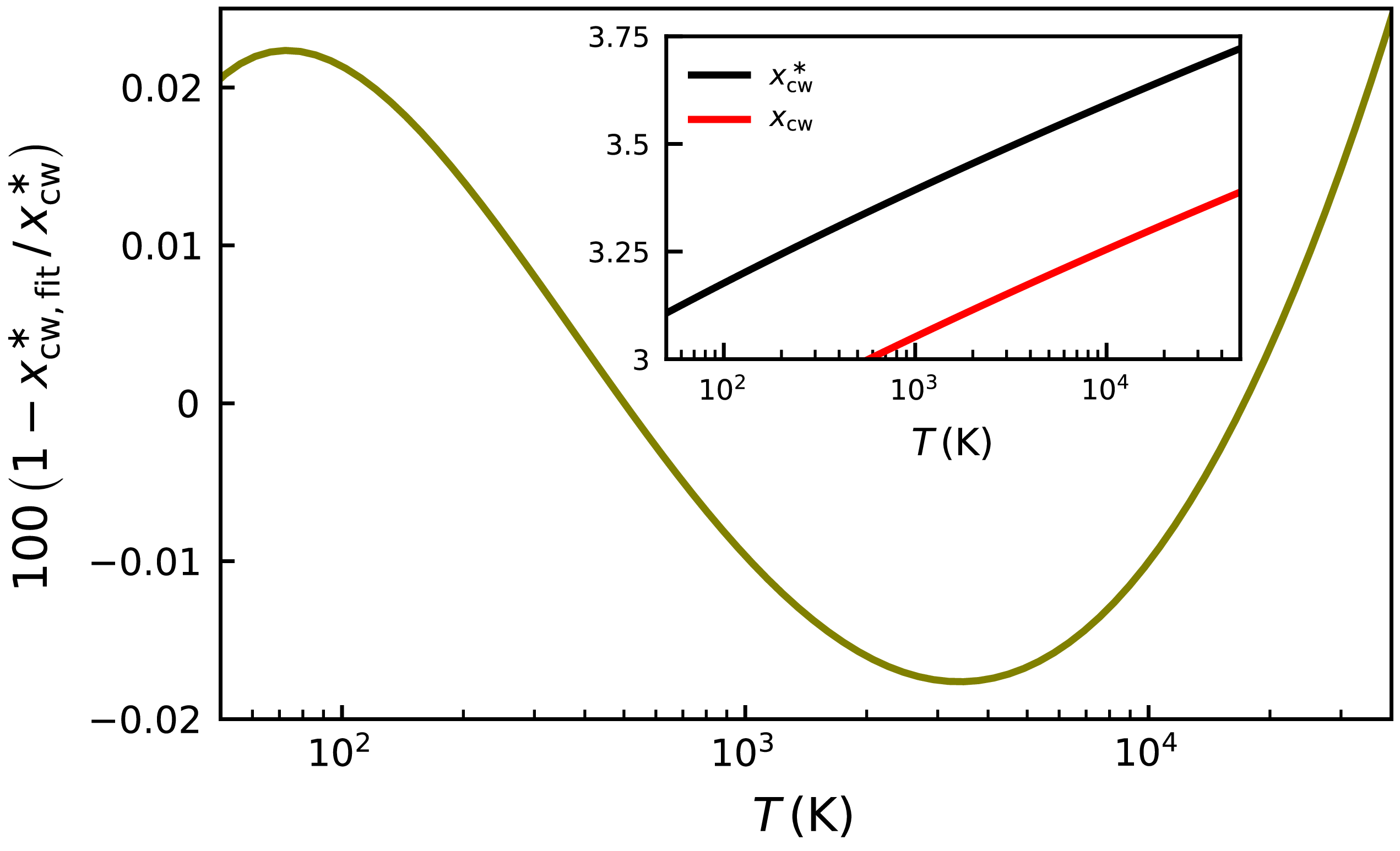
 xcw

 ttrap,x
 τ0
 T=104K
 xcw∗
 ttrap
 <|x|
 ftrap

 Nscat,x
 τ0
 τ0
 T=104K
 xcw∗
 fscat,<|x|

 Nscat, wing
 τ0
 T=104K
 Nscat,wing

 Nscat, last excursion
 T=104K


 MF,x
 τ0
 T=104K
 xcw∗
 MF
 <|x|
 fMF,<|x|

 MF,x
 τ0=107
 T=104K
 α

 3Prad,x/urad,x
 τ0=106
 τ0=107
 τ0=108
 r/R
 T=104K
 105

 ≥|x|
 fesc,x
 (aτ0)1/3
 τ0

 τ0
 α
 |x|
 xcw∗

 α
 |x|
 xcw∗
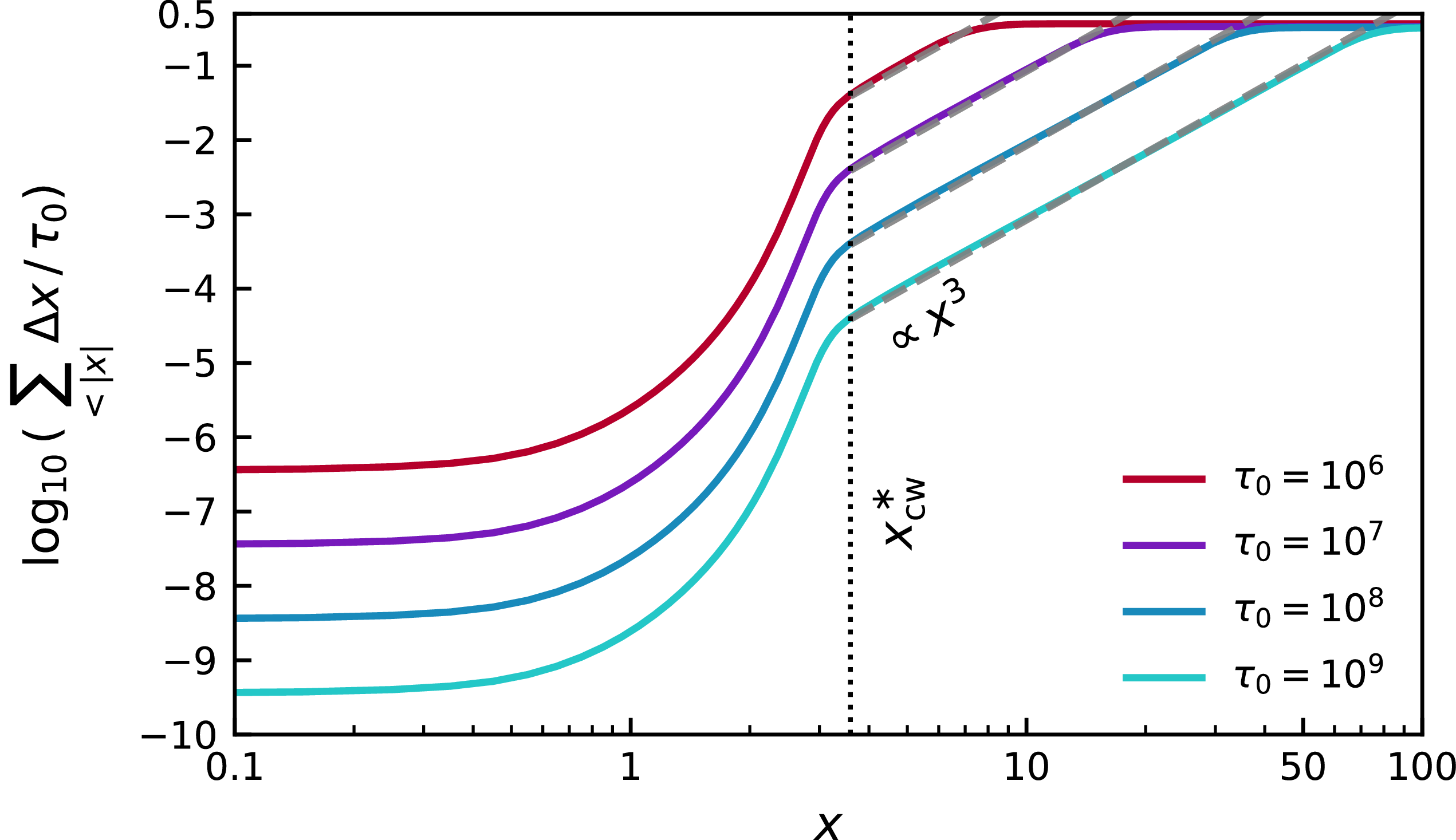
 α
 |x|
 xcw∗

 α
 |x|
 xcw∗
 xesc≈(aτ0)1/3

 ℓjump
 τ0
 T=104K
 p(ℓjump/R)
 1/τ0
 1−P(<ℓjump)=P(>ℓjump)
 >
 ℓjump
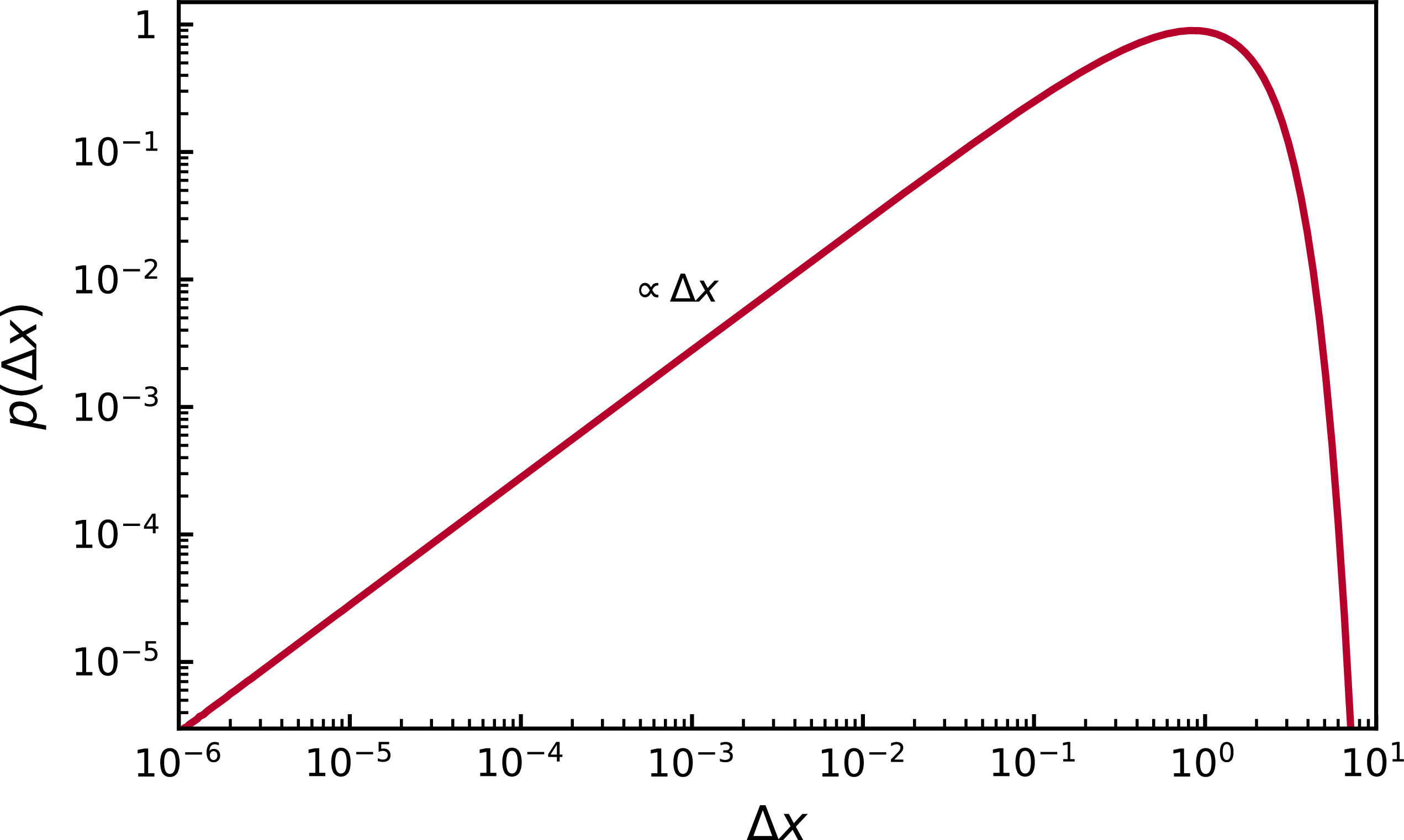
 p(Δx)
 τ0=107
 T=104
 τ0

 T=104K
 xcw∗
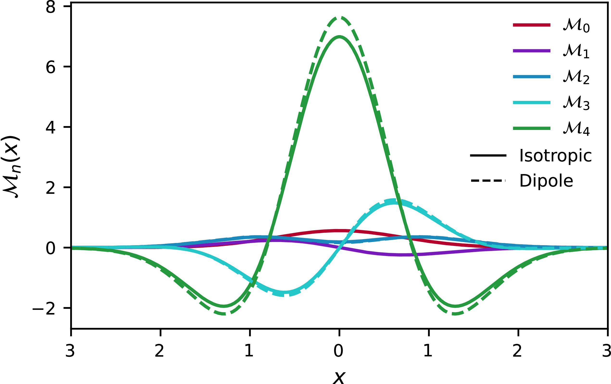
 RII
 Mk

 M2
 xcw∗
 |M2−M0|
 |M2−M0|/M0
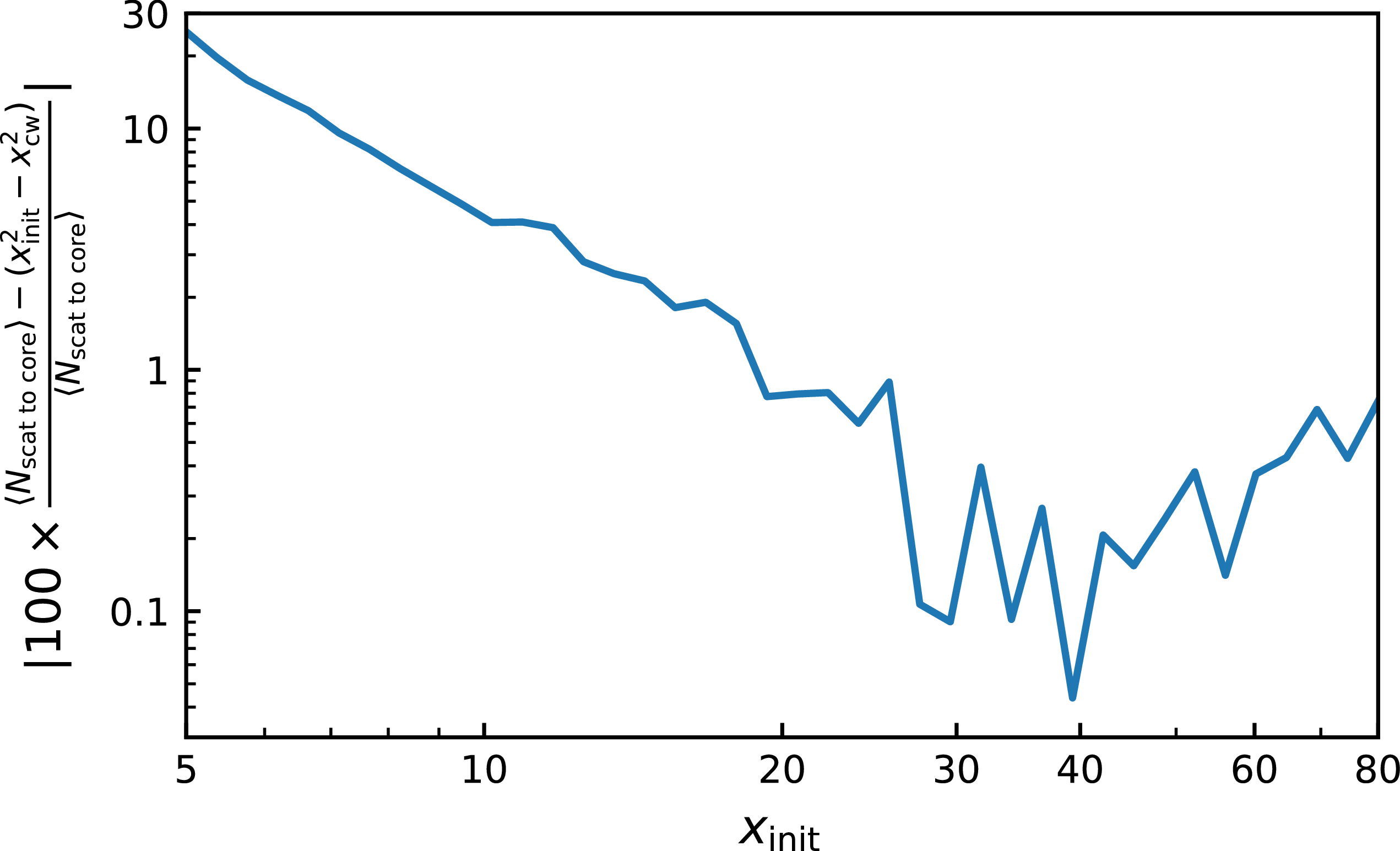
 xinit
 ≤1%
 5×10⁷
 x=5
 x=80
 T=104K

 P(Nscat)
 xinit
 Nscat
 ∝Nscat−1.5
 ≤Nscat
 xinit

 Open access

