





1. Introduction
Radio pulsars have long been of scientific interest for their wide-ranging phenomenology and for their ability to reveal physical properties of matter at high density and verify properties of general relativity. For example, a comprehensive list of pulsar observed properties is given in the Australia Telescope National Facility’s (ATNF) pulsar catalogue (Manchester et al. Reference Manchester, Hobbs, Teoh and Hobbs2005), which now includes
 $\sim$
4 000 pulsars. Polarimetry measurements of pulsars (Johnston & Kerr Reference Johnston and Kerr2018) are an important input for models on how radio pulsations are produced.
Understanding the birth and evolution of single pulsars (Faucher-Giguère & Kaspi Reference Faucher-Giguère and Kaspi2006) and of pulsars in binary systems (Bhattacharya & van den Heuvel Reference Bhattacharya and van den Heuvel1991) are important for constraining stellar evolution in general and for understanding interactions and mass transfer in binary systems (Verbunt Reference Verbunt1993). For constraining nuclear physics and physics of matter under high densities which occur inside neutron stars mass measurements are required, including for binary radio pulsars (Thorsett & Chakrabarty Reference Thorsett and Chakrabarty1999). Here we take an observational approach and consider what the new Evolutionary Map of the Universe (EMU) and Polarisation Sky Survey of the Universe’s Magnetism (POSSUM) radio sky surveys can tell us about radio pulsars.
Because pulsars are compact sources, they show flux variability caused by diffractive and refractive interstellar scintillations (e.g. Rickett et al. Reference Rickett, Coles and Bourgois1984). Kumamoto et al. (Reference Kumamoto2021) carried out a flux density variability survey of 286 radio pulsars with Parkes telescope at 1.4 GHz. One characterisation of the variability is the modulation index, m, defined as
 $m = \sigma_S /S$
with mean flux density S and
 $\sigma_S$
is the standard deviation of the flux densities of a given pulsar. They confirmed that m is inversely correlated with dispersion measure (DM) with large scatter (their Figure 3) and that for DM
 ${\gt}$
100 cm
 $^{-3}$
pc the modulation indices are less than 0.4.
Radio spectrum measurements for pulsars (Izvekova et al. Reference Izvekova, Kuzmin, Malofeev and Shitov1981) are needed to constrain emission mechanisms. Several studies of spectra and spectral indices have been carried out previously. Recent studies include the following. Pulsar flux densities and spectral fits for 281 pulsars were compiled by Maron et al. (Reference Maron, Kijak, Kramer and Wielebinski2000), who find most fit by a simple power-law and about 10% fit by a broken power-law. Jankowski et al. (Reference Jankowski2018) study spectra of 441 pulsars and obtained spectral fits with the following models: simple or broken power law, power law with either low or high-frequency cut-off and log-parabolic spectrum. They find that 79% of the pulsars that could be classified have simple power-law spectra. Measurements for 1 170 pulsars observed by the SARAO MeerKAT radio telescope in multiple epochs (Posselt et al. Reference Posselt2023) enabled measurements of spectra and modulation indices. They also studied correlations among spectral parameters
Identification of new pulsars to increase the known numbers for carrying out population level studies of pulsars and to find interesting individual objects is important. This is becoming possible with new radio telescope facilities. Frail et al. (Reference Frail2024) used the MeerKAT radio telescope to find pulsar candidates. To identify pulsars from the vast numbers (
 $\sim10^5$
to
 $10^7$
) of radio sources, circular polarisation, linear polarisation, in-band spectral index, compactness, variability, and multiwavelength counterparts are used to select pulsar candidates. Dai et al. (Reference Dai2015) measure the multifrequency polarisation pulse profiles for 24 millisecond pulsars and study the variability of polarisation with pulsar rotation phase, which demonstrates that observed polarisation properties in a continuum imaging survey are reduced compared to time-domain observations, thus limiting the ability to search for pulsars by polarisation properties in continuum imaging surveys. The use of flux variability from interstellar scintillations to identify pulsars is discussed in Dai et al. (Reference Dai2016).
The EMU and POSSUM surveys are currently being carried out with the Australian Square Kilometre Array Pathfinder (ASKAP) telescope (Johnston et al. Reference Johnston2008; Hotan et al. Reference Hotan2021). The EMU survey has a frequency band 288 MHz wide centred at 943 MHz and is producing the state-of-the-art radio atlas of the southern sky for a wide array of scientific goals (Hopkins et al. Reference Hopkins2025). EMU will have a larger sky coverage than previous surveys combined with high sensitivity. The POSSUM survey (Gaensler et al. 2025) is being carried out to measure the polarisation and rotation measure (RM) properties of a wide range of extragalactic and Galactic objects and to contribute interferometric data with excellent surface brightness sensitivity, which can be combined with single-dish data to study the diffuse Galactic interstellar medium.
A related work (Ahmad et al. Reference Ahmad2025) analyses EMU data to search for radio pulsars using the variance imaging method (Dai et al. Reference Dai2016; Dai et al. Reference Dai, Johnston and Hobbs2017). That work analysed 16 EMU observations (fields) covering
 $\sim$
480 square degrees of high Galactic latitude sky containing 59 800 compact radio sources. 20 variable sources were found, including 9 known pulsars, 1 radio star, 1 ultra-long period source, 3 radio star candidates and 6 pulsar candidates. The aim of the current work is, instead, to analyse known radio pulsars to determine which pulsar properties can be measured using the EMU and POSSUM surveys, and what we can learn from these measurements.
Here we carry out a pilot study of radio pulsars using 28 fields of observations for the EMU and POSSUM surveys. We identify known radio pulsars in the same sky area from the ATNF pulsar catalogue, and measure their basic properties, discussed in Section 2. Then we describe the measured pulsar properties, including RMs and flux densities/spectra in Section 3. We discuss the implications of the new measurements in Section 4, and give a brief summary in Section 5.
2. Data and analysis
2.1. Observations
ASKAP is a radio interferometer consisting of 36 dishes, each with 12 m diameter, located at Inyarrimanha Ilgari Bundara, CSIRO’s Murchison Radio-astronomy Observatory, Western Australia (Hotan et al. Reference Hotan2021). The dishes have phased-array feeds, each of which forms 36 dual-polarisation beams. This provides ASKAP with a
 $\sim$
30 square degrees area field of view. EMU is an all-sky survey with ASKAP which has the goal of making deep radio continuum maps covering the southern sky
 $-90^{\circ}\leq DEC \leq +10^{\circ}$
(Hopkins et al. Reference Hopkins2025). POSSUM (Gaensler et al. 2025) is a commensal survey with EMU which adds polarisation measurements so combined, EMU and POSSUM capture full Stokes information. The surveys have a central frequency of 943 MHz and a bandwidth of 288 MHz with 1 MHz-wide channels and integration time for a typical observation of 10 h, thus obtaining a Stokes I sensitivity of
 $\sim$
20–30
 $\mu$
Jy beam
 $^{-1}$
.
Each observation is given a unique schedule block (SB) ID. Data processing is carried out using the ASKAPsoft package (Guzman et al. Reference Guzman2019), which includes calibration, flagging, and image generation. A full-Stokes radio continuum image for the field of view is produced and total intensity catalogues and noise maps are generated with Selavy (Whiting & Humphreys Reference Whiting and Humphreys2012). After completing scientific validation, data are uploaded to the CSIRO ASKAP Science Data Archive (CASDAFootnote a ) and made publicly available.
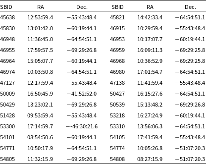
List of observations (SBIDs).

Table 1. Long description
A table titled ‘List of observations (SBIDs)’ with two columns each for SBID, RA, and Dec. The table has 30 rows and 6 columns. Each row presents a unique schedule block ID, right ascension, and declination values. Row 1: SBID 45638, RA 12:53:59.4, Dec 55:43:48.4, SBID 45821, RA 14:42:33.4, Dec 64:54:51.1. Row 2: SBID 45830, RA 13:01:42.0, Dec 60:19:44.1, SBID 46915, RA 10:29:59.4, Dec 55:43:48.4. Row 3: SBID 46948, RA 11:36:45.0, Dec 64:54:51.1, SBID 46953, RA 10:17:07.7, Dec 60:19:44.1. Row 4: SBID 46955, RA 17:59:57.5, Dec 69:29:26.8, SBID 46959, RA 16:09:11.3, Dec 69:29:25.8. Row 5: SBID 46964, RA 15:05:07.7, Dec 60:19:44.1, SBID 46968, RA 10:36:52.9, Dec 69:29:25.8. Row 6: SBID 46974, RA 10:03:50.8, Dec 64:54:51.1, SBID 46980, RA 17:01:54.7, Dec 64:54:51.1. Row 7: SBID 47127, RA 12:17:59.4, Dec 55:43:48.4, SBID 47138, RA 11:41:59.4, Dec 55:43:48.4. Row 8: SBID 50009, RA 16:50:45.9, Dec 41:52:52.0, SBID 50427, RA 16:15:27.6, Dec 64:54:51.1. Row 9: SBID 50429, RA 13:23:02.1, Dec 69:29:26.8, SBID 50539, RA 15:13:48.2, Dec 69:29:26.8. Row 10: SBID 51428, RA 09:53:59.4, Dec 55:43:48.4, SBID 53218, RA 16:27:24.9, Dec 60:19:44.1. Row 11: SBID 53300, RA 17:14:59.7, Dec -46:30:21.6, SBID 53310, RA 13:56:06.3, Dec 64:54:51.1. Row 12: SBID 54101, RA 08:54:50.6, Dec 60:19:44.1, SBID 54105, RA 17:41:59.4, Dec 55:43:48.4. Row 13: SBID 54771, RA 10:50:17.9, Dec 64:54:51.1, SBID 54774, RA 10:05:26.8, Dec 51:07:20.3. Row 14: SBID 54805, RA 11:32:15.9, Dec 69:29:26.8, SBID 54808, RA 08:27:15.9, Dec 51:07:20.3.
EMU Stokes I image of field centred on R.A. 10 H 17 M DEC
 $-60^{\circ}$
, image ID SB46953, with locations of ATNF Pulsars marked by green circles.

2.2. EMU/POSSUM data and ATNF catalogue
We consider 28 EMU/POSSUM fields within 10
 $^{\circ}$
of the Galactic plane. These are listed in Table 1 with the coordinates of their centres. The fields each cover a sky area of
 $\sim6^{\circ}$
by 6
 $^{\circ}$
with circular beam size of 15
 $^{\prime\prime}$
, the standard observing field size and resolution for the EMU and POSSUM surveys (Hopkins et al. Reference Hopkins2025). Each field consists of 288 images of 1 MHz bandwidth centred on 943 MHz. These are processed by the EMU and POSSUM pipelines to produce a 288 MHz bandwidth Stoke I image and full Stokes cubes (1 MHz channels). The standard pipelines also produce an EMU catalogue and a POSSUM catalogue for each field, with more details given in Hopkins et al. (Reference Hopkins2025) and Gaensler et al. (2025).
We also carried out a custom processing for the 28 fields which produced the following for each field: a continuum (Stokes I) image, Stokes Q and U images, a Faraday depth (FD) cube, a polarised intensity image and an image of RM at the peak FD value for each pixel.
The ATNF pulsar database was downloaded on March 22, 2024, consisting of properties for 3 474 pulsars. The properties for each pulsar include the pulsar name, position and other parameters. See the ATNF online Catalogue for definitions of the parameters. From the ATNF catalogue we included only those pulsars that had observed radio emission.
2.3. Analysis
One of the EMU field Stokes I images is shown in Figure 1. The first pass of the analysis was to determine which ATNF pulsars were within each image, with the second pass to determine whether they were within the area covered by the EMU and POSSUM catalogues. The latter area is less than the full area of the image because of a region around the edge of the image which is not included in the catalogues, because of its lower sensitivity. The second step was carried out by additionally matching the ATNF pulsar positions with the source positions from the EMU catalogue on the Stokes I image. Typically there were a few ATNF pulsars in each field, but 25 000–30 000 EMU catalogue sources in each field.
As an exploratory step, we separated out the non-radio emitters from the ATNF catalogue. This list was reduced to those that have position errors of 10 arcsec or less, then position matched with the EMU catalogues of radio sources (29 catalogues, one per observation with each catalogue containing 25 000–30 000 sources). There were no matches found between the EMU 943 MHz sources and non-radio emitting pulsars.
To match the pulsars with catalogue sources, we obtained the position errors from the ATNF catalogue: 3 have large errors (2 with error
 ${\gt}400^{\prime\prime}$
, 1 with no error listed) thus those 3 pulsars were omitted from further consideration. The remaining pulsars in the catalogue area have errors below 10
 $^{\prime\prime}$
(3.7 micro
 $^{\prime\prime}$
to 9.7
 $^{\prime\prime}$
). The pulsar position matches were carried out with EMU/POSSUM catalogues keeping matches up to 10
 $^{\prime\prime}$
.
We determined which ATNF pulsars were inside the area of the fields covered by the catalogues. For an ATNF pulsar to have properties included in the EMU and POSSUM catalogues, it had to match a catalogue source. The total number of pulsars in the catalogue area was 210. Of these 159 pulsars were detected and matched a catalogue source. 24 pulsars were detected by manual inspection in the catalogue region but were not in the catalogue; and 27 pulsars had no detection in the catalogue region or in the catalogue.
Of the 159 pulsars, 8 had measurements in two different EMU/POSSUM observations. The 28 EMU/POSSUM images have between 0 pulsars and 24 pulsars each. The two largest separations between the ATNF and EMU positions are 7.6
 $^{\prime\prime}$
and 8.8
 $^{\prime\prime}$
, both having pulsar position errors of 5.7
 $^{\prime\prime}$
. Thus, all matches are consistent with real matches (maximum difference
 ${\lt}2$
times the
 $1\sigma$
position error).
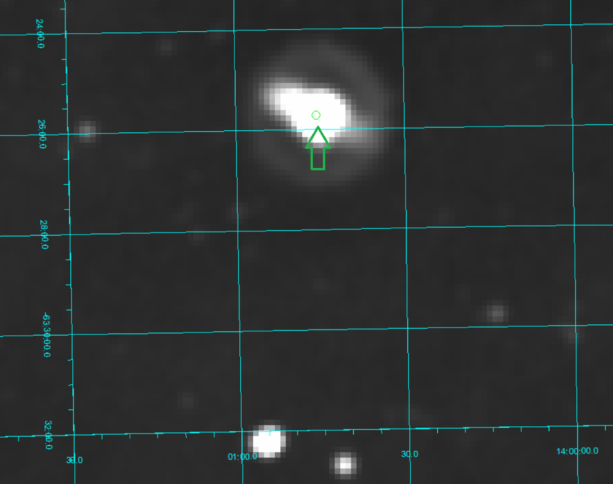
In summary, a high fraction of the ATNF pulsars in the images were detected (183 of 210), and a high fraction are found in the EMU catalogues (159 of 210 or 75%). Most are consistent with unresolved point sources, but some are clearly extended (see Figure 2), and others were consistent with a point source embedded within bright extended emission (see Figure 3). For the cases with significant source extension at 943 MHz (17 of the 159 pulsars) at least a significant fraction of the flux density must be coming from the emission surrounding the pulsar, either associated with the pulsar or along the same line-of-sight.Footnote b
3. Measured pulsar properties
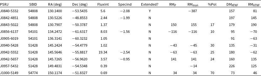
A summary of the measured properties of the 159 pulsars studied here is given in Table 2. Only the first 10 pulsars are listed here, the full set of 159 are in the on-line Table.
Example of an extended source associated with the ATNF pulsar J1400-6325 (green circle with arrow, upper centre of image).

Example of a point-like source associated with the ATNF pulsar J1016-5857 (green circle with arrow, upper right of image) embedded in extended emission.

Properties of EMU/POSSUM pulsar sample.
 $^{\rm a,b}$

Table 2. Long description
A table with 10 rows and 12 columns detailing properties of pulsars detected in a survey. The columns are labeled as PSRJ, SBID, RA (deg), Dec (deg), Fluxint, Specind, Extended?, RMp, RMman, %Pol, DMATNF, and RMATNF. Each row lists specific values for these properties. For example, Row 1: PSRJ, J0840-5332; SBID, 54808; RA (deg), 130.1400; Dec (deg), -53.5435; Fluxint, 5.6; Specind, -2.08; Extended?, Y; RMp, -387; RMman, 157; %Pol, 81; DMATNF, 157; RMATNF, 81.
 $^{\rm a}$
The first 10 entries are shown here. The full Table is published online.
 $^{\rm b}$
The column names are: SBID- observation number; Fluxint- integrated flux density; Specind: in-band spectral index; Extend?- Y: has extended emission, N: consistent with a point source; RM
 $_P$
- rotation measure in the POSSUM catalogue; RM
 $_{\rm man}$
- rotation measure extracted manually; %Pol- percent linear polarisation; DM
 $_{\rm ATNF}$
and RM
 $_{\rm ATNF}$
- dispersion measure and rotation measure from the ATNF online pulsar catalogue.
3.1. Pulsars with two EMU/POSSUM observations
There were eight pulsars observed at two different times in the EMU data. Four had 943 MHz flux density measurements consistent (
 ${\lt}3\sigma$
) between the two observations (B1110-65, J1019-5749, J1415-6621 and J1700-4422) and four had strong evidence for 943 MHz flux density variations: J1035-6720 (5.6
 $\sigma$
difference), J1047-6709 (24.4
 $\sigma$
), J1056-7117 (7.4
 $\sigma$
) and J1137-6700 (7.6
 $\sigma$
).
3.2. Rotation measures
RMs are listed for many pulsars (105 of the 159) in the ATNF catalogue (hereafter RM
 $_{\rm ATNF}$
). We measure RM using two methods here. The first is to extract the FDpeak_fit value (called RM
 $_{\rm POSSUM}$
here) from the POSSUM catalogue sources matched to the pulsars, yielding 81 RM values. The second method was to extract the RM value from the custom processing of the POSSUM Stokes cubes (called RM
 $_{\rm manual}$
here). This yielded 121 pulsars with RM values. Thus the largest number of RM values is RM
 $_{\rm manual}$
.
For the 54 of the 159 pulsars in the ATNF catalogue that have no listed RM value, 29 have RM
 $_{\rm manual}$
and 6 have RM
 $_{\rm POSSUM}$
, and the 6 with RM
 $_{\rm POSSUM}$
also have RM
 $_{\rm manual}$
. For all cases, RM
 $_{\rm POSSUM}$
and RM
 $_{\rm manual}$
values agree. Figure 4 shows RM
 $_{\rm manual}$
and RM
 $_{\rm POSSUM}$
compared to RM
 $_{\rm ATNF}$
. For a few pulsars we find different values for RM
 $_{\rm manual}$
than RM
 $_{\rm ATNF}$
. These could be caused by a source brighter than the pulsar along the same line-of-sight (behind or in front of the pulsar) that has a different RM than the ATNF pulsar. The four with different RM (in units of rad/m
 $^2$
) are: B0839-53 with RM
 $_{\rm manual}$
= −386.9, RM
 $_{\rm ATNF}$
=+81; J0957-5432 has RM
 $_{\rm manual}$
= −14, RM
 $_{\rm ATNF}$
=+125; J1415-6621 has RM
 $_{\rm manual}$
= +18.8, RM
 $_{\rm ATNF}$
=+302; and J1709-4401 has RM
 $_{\rm manual}$
= −48.1, RM
 $_{\rm ATNF}$
=−122.
New measurements of rotation measure (RM, in units of rad/m
 $^2$
) from POSSUM (vertical axis) vs. RM (in units of rad/m
 $^2$
) from the ATNF catalogue (horizontal axis). New RMs were obtained for 29 ATNF pulsars which had no previous RMs. RM values of 0 mean no measurement (for both horizontal and vertical axes).

3.3. Spectral indices
3.3.1. Multi-band spectral indices
Initially, 2-band spectral indices were computed from the 943 MHz flux densities in the EMU catalogue compared to (a) the ATNF 400 MHz flux densities (43 cases) and (b) 1 400 MHz flux densities (158 cases) in the ATNF catalogue. As a more reliable method for measuring multi-band spectral indices, the pulsar_spectra software package was used (Swainston et al. Reference Swainston, Lee, McSweeney and Bhat2022). pulsar_spectra contains a database of pulsar flux measurements and it allows a user to add their own flux density measurements then fit and show the spectrum of a given pulsar. Thus, we added the flux density for each pulsar from EMU. For pulsars with
 $\ge$
4 measurements, a power law (PL) spectrum is fit; for those with
 $\ge$
5, a high frequency cutoff power law (HFCO) is also fit; for those with
 $\ge$
6, a broken power-law (BPL) and a low frequency turn-over power law (LFTO) are also fit; for those with
 $\ge$
7 a double turnover spectrum (DTO) is also fit. The best fit model among those fitted is chosen using the Akaike information criterion (AIC), with details given in Swainston et al. (Reference Swainston, Lee, McSweeney and Bhat2022).
For the 159 pulsars, we obtained best-fit spectra using pulsar_spectra, where we fit the 8 pulsars with 2 EMU 943 MHz measurements twice, once for each measurement. 58 pulsars were fit best with a PL; 12 pulsars were fit best with a LFTO; 11 pulsars were fit best with a BPL; 9 pulsars were fit best with a HFCO; none were fit best by a DTO.
An example PL fit and an example BPL fit are shown in Figure 5. Most fits with several (
 ${\gt}5$
) measurements show the following features: the overall fit looks quite reasonable; there are several flux density measurements that do not agree with the fit (outliers) and often two different measurements at nearly the same frequency that do not agree. The number of outliers is typically 20% to 60% of the number of flux densities.
Example fits to the multi-band fluxes of the pulsars. The top panel shows a power law fit to the flux densities of J0940-5428, and the lower panel shows a broken power law fit to the flux densities of J0942-5552. Most pulsars have several outlier fluxes which do not match the fit.

For the remaining pulsars with
 ${\lt}$
4 flux density measurements, we fit a power law model. These consisted of 77 cases with 2 flux densities and 2 cases with 3 flux densities. For these cases there were no flux density outliers.
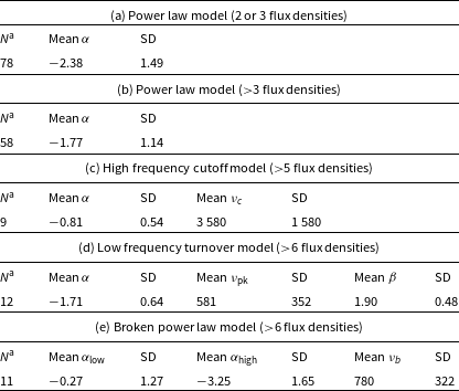
Multi-band spectral index statistics.

Table 3. Long description
A table comparing spectral index statistics across different models and flux densities. The table has five sections, each representing a different model. Each section includes the sample size (N), mean, and standard deviation (SD) for various parameters. Panel A: Power law model (2 or 3 flux densities) with 78 samples, mean alpha of 2.38, and SD of 1.49. Panel B: Power law model (>3 flux densities) with 58 samples, mean alpha of 1.77, and SD of 1.14. Panel C: High frequency cutoff model (>5 flux densities) with 9 samples, mean alpha of 0.81, SD of 0.54, mean nu_c of 3580, and SD of 1580. Panel D: Low frequency turnover model (>6 flux densities) with 12 samples, mean alpha of 1.71, SD of 0.64, mean nu_pk of 581, SD of 352, mean beta of 1.90, and SD of 0.48. Panel E: Broken power law model (>6 flux densities) with 11 samples, mean alpha_low of 0.27, SD of 1.27, mean alpha_high of 3.25, SD of 1.65, mean nu_b of 780, and SD of 322.
 $^{\rm a}$
N is the sample size.
The summary statistics of the spectral indices from the model fits to the multi-band flux densities are given in Table 3. The included fits are those that converged and produced a best-fit model. The different cases are shown: the power law fits to 2 or 3 flux densities; the more reliable power law fits to
 ${\gt}3$
flux densities; the high frequency cut-off model fits; the low frequency turn-over model fits; and the broken power law model fits.
The EMU 943 MHz flux densities were outliers for eight of the 90 cases with
 ${\gt}3$
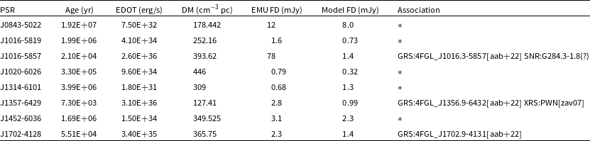
flux densities, with the EMU flux density above the model for seven cases and below for one case. For one additional case, J1019-5749, one EMU measurement was above the model and the other EMU measurement agreed with the model. Properties, including age, spindown energy loss rate and DM, of these eight outliers are listed in Table 4. Of the eight outliers, three are young (spindown age
 ${\lt}10^5$
yr) and are associated with a gamma-ray source. These three also have high spindown power (
 ${\gt}3\times10^{35}$
erg/s).
As noted in Section 3.1, of the eight pulsars with two 943 MHz measurements, four had significant (
 ${\gt}5\sigma$
) flux density variations. ISM refractive and diffractive scintillations could be the cause of the flux density variations of a factor of up to a few, as explained by Kumamoto et al. (Reference Kumamoto2021). This would be consistent with both EMU and other instruments having a significant fraction of flux densities off the best fit model regardless of model type.
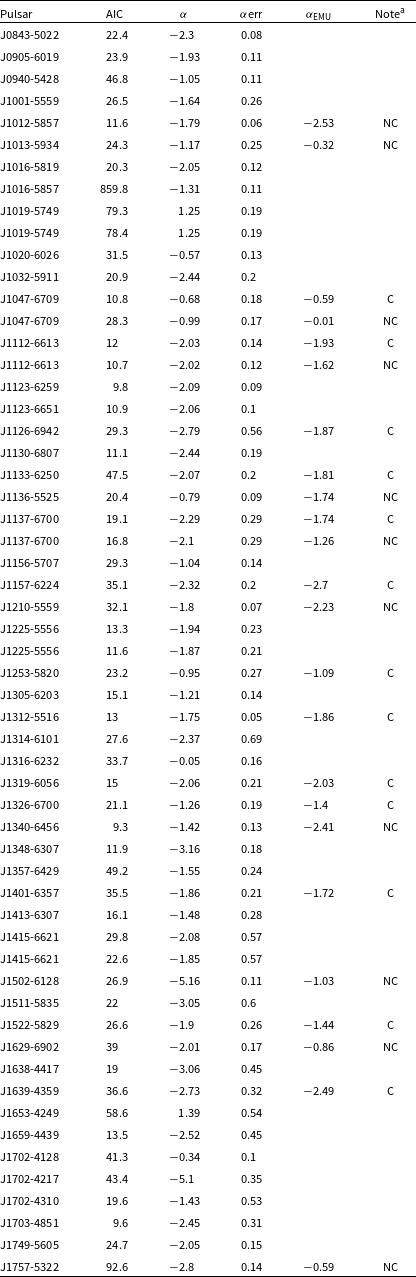
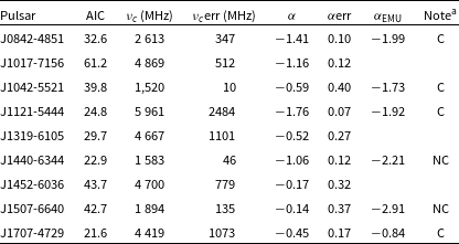
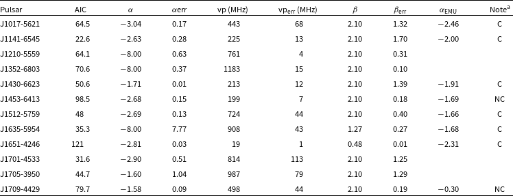
The resulting best fit models for the cases with
 ${\gt}3$
flux densities are shown: for the PL model in Table 5; for the HFCO model in Table 6; for the LFTO model in Table 7; and for the BPL model in Table 8.
3.3.2. EMU in-band spectral indices
The EMU catalogues include in-band spectral indices for approximately 1/3 of the brightest sources, but do not include in-band spectral index errors. 53 of the 159 pulsars had in-band spectral indices. The mean EMU in-band 943 MHz spectral index (
 $\alpha_{943}$
) is
 $-1.54$
with a standard deviation (SD) of 1.04.
The EMU in-band spectral indices were compared to the spectral model fits to the multi-band flux densities. The multi-band spectral indices have different meanings for the different spectral models. For the PL model the in-band and PL spectral index have the same meaning. For the BPL model, depending on the break frequency, the EMU index should be either equal to the low frequency index, the high frequency index or in-between the two. For the HFCO model, if the cutoff frequency is
 ${\gt\gt}$
943 MHz the EMU index should be the spectral index and if the cutoff frequency is near or below 943 MHz the EMU index should be steeper (more negative) than the HFCO index. For the LFTO model, if the turn-over frequency is
 $\lt\lt$
943 MHz the EMU index should agree with the LFTO index and if the turn-over frequency is near or above 943 MHz the EMU index should be flatter (more positive) than the LFTO index.
We examined all spectral fits with
 ${\gt}3$
fluxes and determined whether the EMU in-band spectral index was consistent with the multi-band model fit. For the 53 cases with both EMU spectral index and multi-band model fits (
 ${\gt}3$
fluxes): 2 model fits were bad (clear disagreement with flux densities) and 4 model fits had
 $\sim \gt$
50% of the data off the model, thus 6 model fits were judged as not reliable. Another 3 cases were time variable in EMU data and had one of the two EMU measurements off the model fit. The remaining 44 cases had EMU spectral index consistent with the fit model (within 2
 $\sigma$
) for 31 cases and inconsistent with the fit model for 13 cases. Thus the majority (
 $\simeq$
70%) of the EMU spectral indices agree with the multi-band spectral index of the fit models.
4. Discussion
4.1. Rotation measures
216 pulsars from the ATNF catalogue are located in the region analysed here, of which 159 (74%) are in the EMU/POSSUM catalogues of sources. The EMU survey (Hopkins et al. Reference Hopkins2025) will cover 2
 $\pi$
sr (50%) of sky, giving an estimated pulsar EMU/POSSUM set of
 $\sim$
2 500 of the
 $\sim$
3 500 in the ATNF catalogue. New RM measurements were obtained for 29 pulsars of the 216 in the area covered. The existing number of RM values for the 216 pulsars in the studied area is 105, so the EMU/POSSUM survey, when complete, should increase the number of measured RMs by
 $\sim$
27%. This should enable better modelling of the magnetic field in our Galaxy.
Pulsars for which the EMU flux density was an outlier.

Table 4. Long description
A table with eight rows and seven columns. The columns are labeled PSR, Age (yr), EDOT (erg/s), DM (cm^-3 pc), EMU (mJy), Model FD (mJy), and Association. The table lists properties of pulsars for which the EMU flux density was an outlier. Row 1: PSR, J0843-5022; Age (yr), 1.92E+07; EDOT (erg/s), 7.50E+32; DM (cm^-3 pc), 178.442; EMU (mJy), 12; Model FD (mJy), 8.0; Association, *. Row 2: PSR, J0106-5819; Age (yr), 1.99E+06; EDOT (erg/s), 4.10E+34; DM (cm^-3 pc), 252.16; EMU (mJy), 1.6; Model FD (mJy), 0.73; Association, *. Row 3: PSR, J0106-5857; Age (yr), 2.10E+04; EDOT (erg/s), 2.60E+36; DM (cm^-3 pc), 393.62; EMU (mJy), 78; Model FD (mJy), 1.4; Association, GRS:4FGL_J0106.3-5857[aab+22] SNR:G284.3-1.8(?). Row 4: PSR, J0102-6026; Age (yr), 3.30E+05; EDOT (erg/s), 9.60E+34; DM (cm^-3 pc), 446; EMU (mJy), 0.79; Model FD (mJy), 0.32; Association, *. Row 5: PSR, J1314-6101; Age (yr), 3.99E+06; EDOT (erg/s), 1.80E+31; DM (cm^-3 pc), 309; EMU (mJy), 0.68; Model FD (mJy), 1.3; Association, *. Row 6: PSR, J1357-6429; Age (yr), 7.30E+03; EDOT (erg/s), 3.10E+36; DM (cm^-3 pc), 127.41; EMU (mJy), 2.8; Model FD (mJy), 0.99; Association, GRS:4FGL_J1356.9-6432[aab+22] XRS:PWN[zav07]. Row 7: PSR, J1452-6036; Age (yr), 1.69E+06; EDOT (erg/s), 1.50E+34; DM (cm^-3 pc), 349.525; EMU (mJy), 3.1; Model FD (mJy), 2.3; Association, *. Row 8: PSR, J1702-4128; Age (yr), 5.51E+04; EDOT (erg/s), 3.40E+35; DM (cm^-3 pc), 365.75; EMU (mJy), 2.3; Model FD (mJy), 1.4; Association, GRS:4FGL_J1702.9-4131[aab+22].
4.2. Pulsar spectra
4.2.1. Comparison of spectrum fits with and without EMU flux densities
The EMU flux densities have generally lower uncertainties than other published flux densities: the average EMU 943 MHz flux density of the pulsars was 6.6 mJy, with a mean error of 0.13 mJy. The smaller errors meant that the spectrum type (PL, HFCO, LFTO or BPL) and the spectral parameters were determined better than previously. The exceptions were cases where the EMU flux density was significantly variable, and other cases related to previously published flux densities with a higher fraction of outliers.
Comparing fits including the EMU flux densities (denoted EMU) to fits omitting the EMU flux densities (denoted noEMU), we find the following for best fit spectrum types. PL fits (
 ${\gt}3$
flux densities): 58 EMU cases, 54 noEMU cases; HFCO fits (
 ${\gt}5$
flux densities): 9 EMU cases, 6 noEMU cases; LFTO fits (
 ${\gt}6$
flux densities): 12 EMU cases, 15 noEMU cases; BPL fits (
 ${\gt}6$
flux densities): 11 EMU cases, 2 noEMU cases. For the less reliable power law fits to cases with 2 or 3 flux densities, there were 78 EMU cases and 8 noEMU cases. There were 2 EMU cases and 74 noEMU cases with not enough data to fit.
Power law model (
 ${\gt}3$
flux densities) fit results.

Table 5. Long description
Panel A: Line graph showing the best fit model for the Power Law (PL) model. The x-axis represents an unspecified variable, and the y-axis represents flux densities. The graph includes a trend line indicating the fit of the PL model. Panel B: Line graph showing the best fit model for the High-Frequency Cut-Off (HFCO) model. The x-axis represents an unspecified variable, and the y-axis represents flux densities. The graph includes a trend line indicating the fit of the HFCO model. Panel C: Line graph showing the best fit model for the Low-Frequency Turn-Over (LFTO) model. The x-axis represents an unspecified variable, and the y-axis represents flux densities. The graph includes a trend line indicating the fit of the LFTO model. Panel D: Line graph showing the best fit model for the Broken Power Law (BPL) model. The x-axis represents an unspecified variable, and the y-axis represents flux densities. The graph includes a trend line indicating the fit of the BPL model.
 $^{\rm a}$
C means EMU spectral index consistent within 2
 $\sigma$
of spectral model fit, NC means not consistent within 2
 $\sigma$
.
Including the EMU flux densities in the fits resulted in: 71 cases of no good fit becoming a PL (2–3 data) fit and 7 cases of a PL (2–3 data) fit becoming a PL (
 ${\gt}3$
data) fit. Of the PL (
 ${\gt}3$
data) fits, 3 became LFTO fits, 4 became HFCO fits and 5 became BPL fits. Of the LFTO fits, 2 became PL (
 ${\gt}3$
data) fits, 1 became HFCO fit and 4 became BPL fits. Of the HFCO fits, 1 became PL (
 ${\gt}3$
data) fit, 1 became LFTO fit and 0 became BPL fits. Lastly, of the BPL fits, 0 became PL (
 ${\gt}3$
data) fits, 1 became LFTO fit and 0 became HFCO fits. Thus overall a significant number (22 pulsars) changed fit type of the 159 cases.
We compare the cases which had (more reliable) PL fits (
 ${\gt}3$
data) without and with the EMU flux densities. For fits without the EMU data, the mean PL spectral index was
 $-1.62$
(standard deviation 1.00) with a mean index error 0.30. For fits with the EMU data, the mean PL spectral index was
 $-1.77$
(standard deviation 1.15) with a mean index error of 0.24. Thus, the index errors were reduced and the mean overall spectral index steepened. The difference in mean spectral index is significant at 2.9
 $\sigma$
.Footnote
c
Herafter we use the spectral fits including EMU flux densities.
4.2.2. Spectral fit indices compared to EMU in-band spectral indices
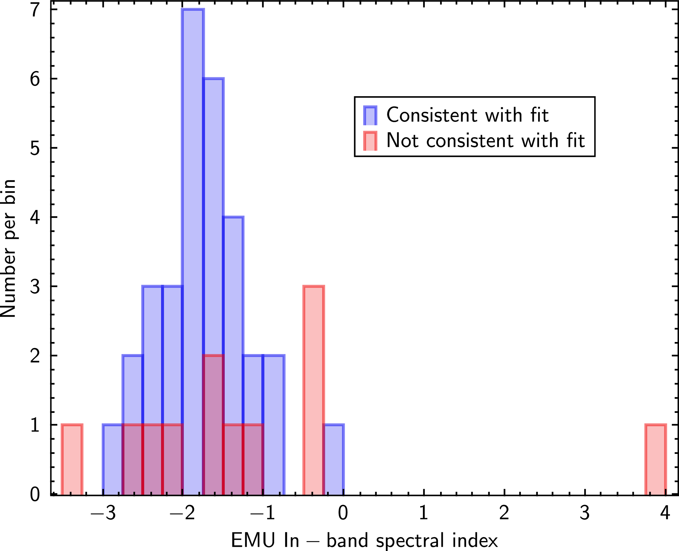
The distribution of EMU in-band spectral indices consistent with the spectral fits (Figure 6) shows a nearly Gaussian distribution centred on an index of
 $-1.9$
, but the values inconsistent with the spectral fits are scattered between
 $-4$
and
 $+4$
. A possible cause is the same as the cause of the flux outliers discussed in Section 3.3.1: frequency-dependent flux density time variability of the pulsars caused by refractive and diffractive scintillations.
To search for other causes for the outliers in EMU in-band spectral index, the two sets (consistent and inconsistent spectral indices) were examined as functions of source size (to check for extended emission), of dispersion measure (to check interstellar scintillations) and of other properties (such as RM, deconvolved major axis and spin-down age). For EMU, a source is detected as extended if the deconvolved major axis is greater than
 $\sim$
7 arcsec (half the spatial resolution). If the presence of a pulsar wind nebula affected the 943 MHz flux density or 943 MHz spectral index and not the multi-frequency measurements, we would expect to find a correlation with source size. We did not find any property that correlated with whether the EMU in-band spectral index agreed with the spectral fit or not.
High frequency cutoff model (
 ${\gt}5$
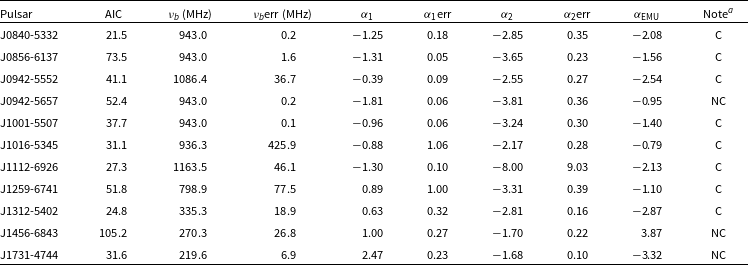
flux densities) fit results.

Table 6. Long description
The table presents model fit results for various cases with flux densities. It includes columns for AIC, alpha, alpha error, and alpha SMU, along with notes. The table has 75 rows and 6 columns. Each row represents a different model fit result. The columns are labeled as follows: AIC, alpha, alpha error, alpha SMU, and Note. The values in the columns represent the specific parameters and results of the model fits. Notable trends or outliers are not explicitly mentioned in the table.
 $^{\rm a}$
C means EMU spectral index consistent within 2
 $\sigma$
of spectral model fit, NC means not consistent within 2
 $\sigma$
.
4.2.3. General results from the spectral fits
The examination of the radio flux density measurements for the 159 pulsars observed in this pilot study shows that a significant fraction (
 $\sim$
20% to 60%) of flux density measurements (EMU and published flux densities from other radio telescopes) disagree with any given model fit. Here, the fit models (see Section 3.3.1) include PL, HFCO, LFTO and BPL. Because of the high prevalence of outlier flux densities, we consider the PL fits for cases with only 2 or 3 flux densities to be significantly less reliable. This leaves 90 (more) reliable spectral fits to examine, 58 for the PL case.
Maron et al. (Reference Maron, Kijak, Kramer and Wielebinski2000) compiled spectra of 281 pulsars with the majority described by a simple power law with average value of spectral index
 $-1.8\pm0.2$
. Spectra of 441 radio pulsars (Jankowski et al. Reference Jankowski2018) were fit the following models: simple or broken power law, power law with either low or high-frequency cut-off and log-parabolic spectrum. The mean index for the simple power law subset was
 $-1.60\pm 0.03$
. Posselt et al. (Reference Posselt2023) carried out power law spectral fits the those pulsars showing weak variability (modulation index
 ${\lt}$
0.13) which was 657 of their total sample of 1 170 pulsars. They found a mean spectral index of
 $-$
1.8 with a standard deviation of 0.8. The different studies find slightly different mean power law indices, but quite different standard deviations. The results here are generally consistent with the previously published results but include a smaller sample of pulsars.
Low frequency turn-over (
 ${\gt}6$
flux densities) fit results.

Table 7. Long description
A table with 8 rows and 8 columns comparing pulsar fit results. The columns are labeled Pulsar, AIC, ν_0 (MHz), ν_0 err (MHz), α, α err, α_EMU, and Note. The table lists specific values for each pulsar under these columns. For example, the first row shows: Pulsar J0842-4851, AIC 32.6, ν_0 2613 MHz, ν_0 err 347 MHz, α -1.41, α err 0.10, α_EMU -1.99, and Note C. The table provides detailed parameters for each pulsar, including their respective errors and notes.
 $^{\rm a}$
C means EMU spectral index consistent within 2
 $\sigma$
of spectral model fit, NC means not consistent within 2
 $\sigma$
.
We found no correlation of spectral fit type with other properties such as dispersion measure, RM or EMU spectral index. A detailed investigation of correlations among power-law spectral index and other pulsar properties was carried out by Posselt et al. (Reference Posselt2023). They found weak but significant correlations between parameters. The strongest correlation for spectral index was with spin down power (
 $\dot{E}$
). The current sample of 159 pulsars is too small to test the correlations found by Posselt et al. (Reference Posselt2023).
Interstellar scintillations cause typical fractional variations in observed intensities on day to month timescales (Sieber Reference Sieber1982; Romani et al. Reference Romani, Narayan and Blandford1986). To test the effect of variability on spectral fits we simulate variable flux densities then carry out spectral fits. From Kumamoto et al. (Reference Kumamoto2021) the modulation index
 $m=\sigma_S/S$
for 286 pulsars with of their sample (given in their Table 1) had a mean of
 $m_{\rm avg}=0.253$
. For our simulation, flux densities at each observed frequency for a given pulsar were sampled from a Gaussian distribution with mean equal to the observed flux density and standard deviation equal to the mean modulation index times the flux density (
 $\sigma_S=m_{\rm avg}/S$
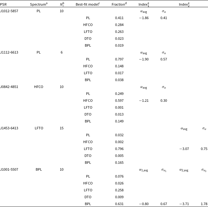
). The simulation was carried out for five pulsars selected from the different best-fit spectral types: PL, HFCO, LFTO and BPL. Two were selected for PL to test the difference in number of observed frequencies. For each pulsar, we created 1 000 simulated spectra (flux densities at all observed frequencies), then fit each spectrum with all models to get 1 000 instances of best-fit model and its spectral parameters.
The results are shown in Table 9. For the two pulsars tested with best-fit PL spectrum, PL was the best-fit model for 41% of the simulated flux densities (J1012-5857) and 80% of the simulated flux densities (J1112-6613). For the best-fit HFCO model (J0842-4851), HFCO was the best-fit model for 60% of the simulated flux densities. For the best-fit LFTO model (J1453-6413), LFTO was the best-fit model for 80% of the simulated flux densities. For the best-fit BPL model (J1001-5507), BPL was the best-fit model for 63% of the simulated flux densities. The results show that variable fluxes, for a pulsar with a typical modulation index of
 $m_{\rm avg}=0.253$
, have a significant effect on the spectral fitting: the best-fit model is robust to flux variations for
 $\sim\!40$
% to
 $\sim\!80$
% of the cases, with overall mean of 65%. This leaves a significant fraction of the simulated spectral (
 $\sim35$
%) giving a different model than the best-fit model to the input observed data.
Thus variability in the flux densities means the individual spectral fits give the initial spectral model only
 $\sim$
65% of the simulations. However for the PL case, the mean spectral index from the simulated spectra (
 $-$
1.88, from top two rows of Table 9) is close to the average spectral index of the fits using the observed flux densities (
 $-$
1.77, case b from Table 3).
Broken power law model (
 ${\gt}6$
flux densities) fit results.

Table 8. Long description
A table comparing pulsar model fit results. The table has 12 rows and 10 columns. Column headers are: Pulsar, AIC, alpha, alpha_err, vp (MHz), vp_err (MHz), beta, beta_err, alpha_EMU, and Note. Row 1: Pulsar, J1017-5621; AIC, 64.5; alpha, -3.04; alpha_err, 0.17; vp (MHz), 443; vp_err (MHz), 68; beta, 2.10; beta_err, 1.32; alpha_EMU, -2.46; Note, C. Row 2: Pulsar, J1141-6545; AIC, 22.6; alpha, -2.63; alpha_err, 0.28; vp (MHz), 225; vp_err (MHz), 13; beta, 2.10; beta_err, 1.70; alpha_EMU, -2.00; Note, C. Row 3: Pulsar, J1210-5559; AIC, 64.1; alpha, -8.00; alpha_err, 0.63; vp (MHz), 761; vp_err (MHz), 4; beta, 2.10; beta_err, 0.31; alpha_EMU, 0.31; Note, C. Row 4: Pulsar, J1352-6803; AIC, 70.6; alpha, -8.00; alpha_err, 0.37; vp (MHz), 1183; vp_err (MHz), 15; beta, 2.10; beta_err, 0.10; alpha_EMU, 0.10; Note, C. Row 5: Pulsar, J1430-6623; AIC, 50.6; alpha, -1.71; alpha_err, 0.01; vp (MHz), 213; vp_err (MHz), 12; beta, 2.10; beta_err, 1.39; alpha_EMU, -1.91; Note, C. Row 6: Pulsar, J1453-6413; AIC, 98.5; alpha, -2.68; alpha_err, 0.15; vp (MHz), 199; vp_err (MHz), 7; beta, 2.10; beta_err, 0.18; alpha_EMU, -1.69; Note, NC. Row 7: Pulsar, J1512-5759; AIC, 48; alpha, -2.69; alpha_err, 0.13; vp (MHz), 724; vp_err (MHz), 44; beta, 2.10; beta_err, 0.40; alpha_EMU, -1.66; Note, C. Row 8: Pulsar, J1635-5954; AIC, 35.3; alpha, -8.00; alpha_err, 7.77; vp (MHz), 908; vp_err (MHz), 43; beta, 1.27; beta_err, 0.27; alpha_EMU, -1.68; Note, C. Row 9: Pulsar, J1651-4246; AIC, 121; alpha, -2.81; alpha_err, 0.03; vp (MHz), 19; vp_err (MHz), 1; beta, 0.48; beta_err, 0.01; alpha_EMU, -2.31; Note, C. Row 10: Pulsar, J1701-4533; AIC, 31.6; alpha, -2.90; alpha_err, 0.51; vp (MHz), 814; vp_err (MHz), 113; beta, 2.10; beta_err, 1.25; alpha_EMU, 1.25; Note, C. Row 11: Pulsar, J1705-3950; AIC, 44.7; alpha, -1.60; alpha_err, 1.04; vp (MHz), 987; vp_err (MHz), 79; beta, 2.10; beta_err, 1.29; alpha_EMU, 1.29; Note, C. Row 12: Pulsar, J1709-4429; AIC, 79.7; alpha, -1.58; alpha_err, 0.09; vp (MHz), 498; vp_err (MHz), 44; beta, 2.10; beta_err, 0.19; alpha_EMU, -0.30; Note, NC.
 $^{\rm a}$
C means EMU spectral index consistent within 2
 $\sigma$
of spectral model fit, NC means not consistent within 2
 $\sigma$
.
Results of spectral fits to pulsars with simulated flux densities.

Table 9. Long description
A table with 12 rows and 11 columns comparing spectral fits to pulsars with simulated flux densities. The columns are labeled as Pulsar, AIC, v_b (MHz), v_b err (MHz), alpha_1, alpha_1 err, alpha_2, alpha_2 err, alpha_EMU, and Note. Each row lists values for different pulsars. Notable trends include variations in AIC values, frequency ranges, and spectral indices. The table provides detailed data on the spectral fits for each pulsar.
 $^{\rm a}$
Best-fit model spectrum using observed flux densities.
 $^{\rm b}N_\nu^{a}$
is number of observed frequencies.
 $^{\rm c}$
Best-fit model spectrum using simulated flux densities.
 $^{\rm d}$
Fraction of the 1 000 simulated spectra which gave this best-fit model.
 $^{\rm e}$
Mean and standard deviation of best-fit spectral index for the model with highest fraction of best-fits. For HFCO this is the PL index of the low frequency part of the spectrum, for LFTO this is the PL index of the high frequency part of the spectrum, for BPL both low frequency index
 $\alpha_{1,{\rm avg}}$
and high frequency index
 $\alpha_{2,{\rm avg}}$
and their standard devations are given.
5. Summary and conclusion
We analysed radio observations from the EMU and POSSUM surveys covering a large area of sky (
 $\sim$
1 000 square degrees) to investigate radio pulsar properties. The EMU and POSSUM products include full Stokes images at 943 MHz with 288 MHz bandwidth and catalogues produced for point sources which were extracted from the images.
Histogram of EMU in-band spectral indices. The pulsars where the EMU spectral index is consistent with the multi-band spectral model fit are shown in blue, the pulsars where the spectral index is not consistent with the fit spectrum model are shown in red.

In the EMU and POSSUM catalogues for this sky area, 159 known pulsars were detected, of which 105 have previously measured RMs. We also carried out custom image processing to produce RM images from which we determined RMs for 29 pulsars without a previous RM.
The uncertainties in the 159 EMU flux densities for these pulsars are, in most cases, smaller than for previously reported flux densities. Eight pulsars were observed at two epochs of which four show variable flux densities (
 ${\gt}5\sigma$
). The EMU flux densities combined with previously measured flux densities at other frequencies and new spectra fits were carried out for the 159 pulsars. The best explanation for outliers in flux-density, which are seen for both EMU and other instruments, is refractive and diffractive interstellar scintillations.
Interstellar scintillations cause typical fractional variations on day to month timescales of
 $\simeq$
25% in observed intensities, thus we simulated the effects of variable flux densities on the spectral fits. The results are that spectral fits with different models yield the input model for
 $\sim\!65$
% of the cases. For simple power-law fits the mean power-law spectral index of a set of pulsars is not strongly affected. This is a major limitation on drawing conclusions from pulsar spectra fits using single epoch observations.
The EMU/POSSUM surveys, when complete, will cover the southern half of the whole sky and are estimated to measure several properties including flux densities and polarisation properties of a large number of pulsars (
 $\sim$
75% of the
 $\sim$
1 800 pulsars). A significant number of pulsars (
 $\sim$
25%) will have RMs measured for the first time.
Acknowledgements
This scientific work uses data obtained from Inyarrimanha Ilgari Bundara, the CSIRO Murchison Radio-astronomy Observatory. We acknowledge the Wajarri Yamaji People as the Traditional Owners and native title holders of the Observatory site. CSIRO’s ASKAP radio telescope is part of the Australia Telescope National Facility (ATNF) (https://ror.org/05qajvd42). Operation of ASKAP is funded by the Australian Government with support from the National Collaborative Research Infrastructure Strategy. ASKAP uses the resources of the Pawsey Supercomputing Research Centre. Establishment of ASKAP, Inyarrimanha Ilgari Bundara, the CSIRO Murchison Radio-astronomy Observatory and the Pawsey Supercomputing Research Centre are initiatives of the Australian Government, with support from the Government of Western Australia and the Science and Industry Endowment Fund. Murriyang, CSIRO’s Parkes radio telescope, is part of the ATNF. We acknowledge the Wiradjuri people as the Traditional Owners of the Observatory site.
Funding statement
This research was supported by a grant from the Natural Sciences and Engineering Research Council of Canada.
Data availability
All data used in this analysis is publicly available through the CASDA or ATNF data archives.


 −60∘

 a,b

 2
 2

 >3
 >5
 >6
 >6

 Open access

