Introduction
The reconstruction of past climate and environmental conditions is of paramount importance for the comprehension of both present and future climate changes (Swetnam et al., Reference Swetnam, Allen and Betancourt1999; Jones and Mann, Reference Jones and Mann2004; Thomas, Reference Thomas2016). Consequently, researchers depend on a variety of natural archives, such as loess–palaeosol sequences (LPS), which serve as continental archives (Kukla, Reference Kukla1978; Kemp, Reference Kemp2001; Terhorst et al., Reference Terhorst, Kühn, Damm, Hambach, Meyer-Heintze and Sedov2014; Lehmkuhl et al., Reference Lehmkuhl, Zens, Krauß, Schulte and Kels2016). These archives yield proxy data that can be used to infer past environmental variations (Buggle et al., Reference Buggle, Hambach, Müller, Zöller, Marković and Glaser2014; Gocke et al., Reference Gocke, Hambach, Eckmeier, Schwark, Zöller, Fuchs, Löscher and Wiesenberg2014; Krauß et al., Reference Krauß, Zens, Zeeden, Schulte, Eckmeier and Lehmkuhl2016; Bösken et al., Reference Bösken, Obreht, Zeeden, Klasen, Hambach, Sümegi and Lehmkuhl2019; Sprafke et al., Reference Sprafke, Schulte, Meyer-Heintze, Händel, Einwögerer, Simon, Peticzka, Schäfer, Lehmkuhl and Terhorst2020; Fischer et al., Reference Fischer, Jöris, Fitzsimmons, Vinnepand, Prud’homme, Schulte and Hatté2021; Vinnepand et al., Reference Vinnepand, Fischer, Jöris, Hambach, Zeeden, Schulte and Fitzsimmons2022). Studies have shown that LPS record both glacial–interglacial climate cycles (Kemp, Reference Kemp2001; Muhs and Bettis, Reference Muhs and Bettis2003; Rousseau et al., Reference Rousseau, Derbyshire, Antoine, Hatté, Elias and Mock2013; Marković et al., Reference Marković, Stevens, Mason, Vandenberghe, Yang, Veres and Újvári2018) and climate changes on a millennial timescale, including the Dansgaard‐Oeschger cycles (Moine et al., Reference Moine, Antoine, Hatté, Landais, Mathieu, Prud’homme and Rousseau2017; Fischer et al., Reference Fischer, Jöris, Fitzsimmons, Vinnepand, Prud’homme, Schulte and Hatté2021; Prud’homme et al., Reference Prud’homme, Fischer, Jöris, Gromov, Vinnepand, Hatté, Vonhof, Moine, Vött and Fitzsimmons2022).
The loess landscape of lower Austria is part of the eastern margin of the European Alps and northern Carpathian Basin loess subdomain, separated only by the Vienna Basin from the Middle Danube Loess Basin (Marković et al., Reference Marković, Stevens, Kukla, Hambach, Fitzsimmons, Gibbard and Buggle2015; Lehmkuhl et al., Reference Lehmkuhl, Nett, Pötter, Schulte, Sprafke, Jary and Antoine2021; Fig. 1). A variety of studies have already been conducted in the area surrounding Langenlois in lower Austria with respect to loess (Piffl, Reference Piffl and Fink1976; Fladerer et al., Reference Fladerer, Havlíček, Roetzel, Salcher, Smolíková and Tuzar2005; Haslinger et al., Reference Haslinger, Smolíková, Havlíček, Roetzel, Heinrich, Holásek, Vachek and Ottner2010; Thiel et al., Reference Thiel, Terhorst, Jaburová, Buylaert, Murray, Fladerer, Damm, Frechen and Ottner2011a; Haesaerts and Damblon, Reference Haesaerts and Damblon2016; Meyer-Heintze et al., Reference Meyer-Heintze, Sprafke, Schulte, Terhorst, Lomax, Fuchs and Lehmkuhl2018; Sprafke et al., Reference Sprafke, Schulte, Meyer-Heintze, Händel, Einwögerer, Simon, Peticzka, Schäfer, Lehmkuhl and Terhorst2020; Boemke et al., Reference Boemke, Einwögerer, Händel and Lehmkuhl2022). The area’s position in a transitional zone between the Atlantic and continental climates (Fink, Reference Fink1956) renders it a particularly compelling subject for palaeoenvironmental studies. Furthermore, the region is distinguished by the presence of numerous archaeological sites embedded in the loess and loess-based palaeosols (Boemke et al., Reference Boemke, Einwögerer, Händel and Lehmkuhl2022 and references therein). These findings range from vast amounts of mammoth bones to settlement structures and human remains from the Gravettian, which were dated between around 31.7 ka cal BP and 26.6 ka BP (Einwögerer et al., Reference Einwögerer, Friesinger, Händel, Neugebauer-Maresch, Simon and Teschler-Nicola2006; Händel et al., Reference Händel, Simon, Einwögerer and Neugebauer-Maresch2009; Marković et al., Reference Marković, Fitzsimmons, Sprafke, Gavrilović, Smalley, Jović, Svirčev, Gavrilov and Bešlin2016). A direct investigation of the loess deposits where they were found, as well as the surrounding area, can provide a more comprehensive understanding of the local palaeoclimate and palaeoenvironmental conditions during these early periods of human occupation. This, in turn, can lead to a more refined understanding of the dispersal of Upper Palaeolithic techno-complexes and the migration of anatomically modern humans within Europe (Kretschmer, Reference Kretschmer2015; Schmidt and Zimmermann, Reference Schmidt and Zimmermann2019).
The loess landscape of lower Austria after Fink (Reference Fink1956) and the locations of the loess–palaeosol sequences in Langenlois and other studies in the region referenced in this paper. An overview map, placing the location in the European loess belt (Lehmkuhl et al., Reference Lehmkuhl, Nett, Pötter, Schulte, Sprafke, Jary and Antoine2021) and showing the last glacial maximum (LGM) extent of glaciers (Ehlers et al., Reference Ehlers, Gibbard and Hughes2011). (Topography from GEOinfo NÖ, loess distribution around Langenlois from GeoSphere Austria).

Figure 1 Long description
The map of lower Austria showing loess distribution, loess landscapes and the locations of study sites. It also includes a topographic representation with elevation in meters above sea level (m a.s.l.). The map identifies three main loess landscapes: ′Dry Loess Landscape,′ ′Transition Loess Landscape,′ and ′Humid Loess Landscape.′ The ′Dry Loess Landscape′ is marked in the northeastern region, while the ′Humid Loess Landscape′ is in the southwest. The ′Transition Loess Landscape′ lies between these two areas. The map also shows the Danube River and its tributary, the Kamp River, flowing through the region. The location of this study's site, Langenlois, and the locations of key loess sites in the region, such as Krems Wachtberg, Großer Buriweg, Ziegelei Hammerer und Kammern-Grubgraben are marked. An inset map in the top left corner provides a broader view of the study area′s location within Europe, showing loess distribution and the extent of the Last Glacial Maximum (LGM) glaciers. A scale bar and north arrow are included for reference.
Reconstructing past climate and environmental conditions from LPS requires the integration of multiple proxies (Frank et al., Reference Frank, Terhorst, Damm, Thiel, Frechen and Peticzka2011; Gocke et al., Reference Gocke, Hambach, Eckmeier, Schwark, Zöller, Fuchs, Löscher and Wiesenberg2014; Krauß et al., Reference Krauß, Zens, Zeeden, Schulte, Eckmeier and Lehmkuhl2016; Meyer-Heintze et al., Reference Meyer-Heintze, Sprafke, Schulte, Terhorst, Lomax, Fuchs and Lehmkuhl2018; Fischer et al., Reference Fischer, Hambach, Klasen, Schulte, Zeeden, Steininger, Lehmkuhl, Gerlach and Radtke2019, Reference Fischer, Jöris, Fitzsimmons, Vinnepand, Prud’homme, Schulte and Hatté2021). Because common parameters applied in loess research reflect a combination of geomorphic and paleoenvironmental influences, combining them has been shown to facilitate the disentangling of distinct influences and the creation of a more detailed and nuanced picture. In this study, we integrate spectrophotometric analysis for high-resolution quantification of colour variations (Debret et al., Reference Debret, Sebag, Desmet, Balsam, Copard, Mourier and Susperrigui2011; Buggle et al., Reference Buggle, Hambach, Müller, Zöller, Marković and Glaser2014; Sprafke, Reference Sprafke2016; Zeeden et al., Reference Zeeden, Krauß, Kels and Lehmkuhl2017), grain-size distribution (GSD) (Schulte et al., Reference Schulte, Sprafke, Rodrigues and Fitzsimmons2018; Újvári et al., Reference Újvári, Kok, Varga and Kovács2016; Vandenberghe, Reference Vandenberghe2013), and geochemical proxies such as weathering indices and elemental ratios (Bokhorst et al., Reference Bokhorst, Beets, Marković, Gerasimenko, Matviishina and Frechen2009; Buggle et al., Reference Buggle, Glaser, Hambach, Gerasimenko and Marković2011; Schatz et al., Reference Schatz, Scholten and Kühn2014; Reiss et al., Reference Reiss, Stüwe, Einwögerer, Händel, Maier, Meng, Pasda, Simon, Zolitschka and Mayr2022; Vinnepand et al., Reference Vinnepand, Fischer, Jöris, Hambach, Zeeden, Schulte and Fitzsimmons2022, Reference Vinnepand, Fischer, Hambach, Jöris, Craig, Zeeden and Thornton2023; Maslov and Podkovyrov, Reference Maslov and Podkovyrov2023). The temporal framework is established through optically stimulated luminescence (OSL) dating.
Despite their significance, the interpretation of LPS remains challenging due to site-specific factors such as reworking, erosion, and local geomorphological influences (Lehmkuhl et al., Reference Lehmkuhl, Zens, Krauß, Schulte and Kels2016; Sprafke, Reference Sprafke2016). These processes can alter GSDs through size-specific sorting and compromise chronological frameworks via sediment hiatuses or secondary relocation. Furthermore, such dynamics may result in the deposition of soil sediments and induce significant spatiotemporal variations in sedimentation rates, necessitating a rigorous assessment of the primary environmental signals. This study investigates three LPS (LLS 1, LLS 2, LAN 4) situated close to one another along a slope. This enables the distinction between the impacts of local sedimentary dynamics and regional climate as recorded in the studied proxies. The regional climate signals can be correlated with other terrestrial climate archives (North Greenland Ice Core Project Members, 2007; Lehmkuhl et al., Reference Lehmkuhl, Zens, Krauß, Schulte and Kels2016; Sprafke et al., Reference Sprafke, Schulte, Meyer-Heintze, Händel, Einwögerer, Simon, Peticzka, Schäfer, Lehmkuhl and Terhorst2020).
By applying a multiproxy, multi-profile approach, we aim to differentiate between sedimentary, pedogenic, and reworking processes reliably. The aim is to correlate the LPS of Langenlois and integrate them into regional and European contexts to obtain a clearer picture of climate and environmental changes during Marine Isotope Stage 2 (MIS 2). The well-documented LPS from Krems-Wachtberg, known for its robust stratigraphic record and archaeological significance (Einwögerer et al., Reference Einwögerer, Friesinger, Händel, Neugebauer-Maresch, Simon and Teschler-Nicola2006; Terhorst et al., Reference Terhorst, Kühn, Damm, Hambach, Meyer-Heintze and Sedov2014; Meyer-Heintze et al., Reference Meyer-Heintze, Sprafke, Schulte, Terhorst, Lomax, Fuchs and Lehmkuhl2018; Sprafke et al., Reference Sprafke, Schulte, Meyer-Heintze, Händel, Einwögerer, Simon, Peticzka, Schäfer, Lehmkuhl and Terhorst2020; Händel et al., Reference Händel, Thomas, Sprafke, Schulte, Brandl, Simon and Einwögerer2021a), serves as a key reference for the regional comparison.
Regional setting and stratigraphy
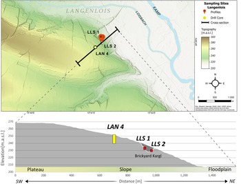
The three LPS are located south of the city of Langenlois (Fig. 2): LLS 1 (48°27′59.7″N 15°41′09.8″E), LLS 2 (48°27′59.7″N 15°41′11.6″E), and LAN 4 (48°27′56.5″N 15°41′03.5″E) (WGS 84). LLS 1 and LLS 2 are located in the pit of the former Kargl brickyard, 40 m apart from each other on the northeast and the southeast walls, respectively. Sediment core LAN 4 was drilled around 150 m farther upslope to the southwest. All sites are located on the loess-covered Early Pleistocene Gobelsburg terrace of the Kamp River at the edge of the river plain (Wessely, Reference Wessely2006). As the palaeo-wind directions in this region are similar to today (Sebe et al., Reference Sebe, Roetzel, Fiebig and Lüthgens2015), the LPS are located on the lee side of the terrace, providing optimal conditions for loess sedimentation during glacial periods (see Boemke et al., Reference Boemke, Einwögerer, Händel and Lehmkuhl2022), making this area a promising site for loess research. Early studies reported significant loess accumulation, with thicknesses of up to 20 m documented at the southern plateau edge (Götzinger, Reference Götzinger1936) and even thicker on the eastern slopes of the Kremsfeld (Piffl, Reference Piffl1955).
Cross section of the slope showing the location of the three sampling sites, LLS 2, LLS 1, and LAN 4, from lowest to highest elevations, respectively. The elevation profile shows the plateau, the sampling on its edge, and the Kamp River floodplain.

Figure 2 Long description
The map shows the area south of the city of Langenlois with topography indicated by shading and a gradient colour scale from 200 to 300 meters above sea level. Sampling sites LLS 1, LLS 2 and LAN 4 are marked. LLS 1 and LLS 2 are identified with profile symbols, while LAN 4 is marked with a drill core symbol. The Kamp River is visible to the east. A cross-section line is drawn through the sampling sites. The cross-section below illustrates the elevation profile from southwest to northeast, showing a plateau, slope and floodplain. Elevation ranges from 200 to 270 meters above sea level. The locations of LLS 1, LLS 2 and LAN 4 are marked on the profile, with LLS 1 and LLS 2 in the Brickyard Kargl and LAN 4 further up the slope. The cross-section highlights the different slope positions for the drill core and the two profiles.
The mean annual temperature in Langenlois is 9.1°C, with an average precipitation of 451.3 mm per year for the period from 1971 to 2000 (ZAMG, n.d). The relatively low precipitation compared with surrounding regions is attributed to the rain shadow effect of the Bohemian Massif, as prevailing winds primarily originate from the northwest (Hiebl et al., Reference Hiebl, Reisenhofer, Auer, Böhm and Schöner2011).
The LPS are located at different elevations. LLS 2, the lowest, is situated 200 m above sea level (m asl), followed by LLS 1 at 201 m asl and LAN 4 at 220 m asl. LLS 1 and LLS 2 have the same slope inclination, whereas LAN 4 is positioned on a less steep section (Fig. 2).
Across Austria, LPS show a west–east gradient in pedogenesis from MIS 3 into MIS 2, positioning Langenlois within the transitional zone (Fink, Reference Fink1956; Terhorst et al., Reference Terhorst, Sedov, Sprafke, Peticzka, Meyer-Heintze, Kühn and Solleiro Rebolledo2015; Sprafke et al., Reference Sprafke, Peticzka, Thiel and Terhorst2024). From the humid loess landscape west of the Bohemian Massif to the dry loess landscape east of the Bohemian Massif, the intensity of pedogenesis generally decreases, both in weathering and in the formation of reduction features, while sedimentation rates increase. In the humid loess landscape, the uppermost Bv horizon developed during the Middle Würmian (Terhorst et al., Reference Terhorst, Frechen and Reitner2002), after which loess–Cryosol units that form under permafrost conditions dominate. In the transitional zone (e.g., Stratzing [Zöller et al., Reference Zöller, Oches and McCoy1994; Thiel et al., Reference Thiel, Buylaert, Murray, Terhorst, Hofer, Tsukamoto and Frechen2011b]; Krems [Terhorst et al., Reference Terhorst, Kühn, Damm, Hambach, Meyer-Heintze and Sedov2014; Meyer-Heintze et al., Reference Meyer-Heintze, Sprafke, Schulte, Terhorst, Lomax, Fuchs and Lehmkuhl2018; Sprafke et al., Reference Sprafke, Schulte, Meyer-Heintze, Händel, Einwögerer, Simon, Peticzka, Schäfer, Lehmkuhl and Terhorst2020]; and Langenlois [Piffl, Reference Piffl and Fink1976; Thiel et al., Reference Thiel, Terhorst, Jaburová, Buylaert, Murray, Fladerer, Damm, Frechen and Ottner2011a]), loess accumulation is significantly higher at the end of the MIS 3 period. Interstadial soils are thin or incipient, and weak pedogenesis and frequent Cryosol horizons persist into MIS 2. Most LPS in this region are located on slopes, resulting in erosional and colluvial overprinting. Farther east in the dry loess landscape (e.g., Stillfried [Peticzka et al., Reference Peticzka, Holawe and Riegler2010; Terhorst et al., Reference Terhorst, Thiel, Peticzka, Sprafke, Frechen, Fladerer, Roetzel and Neugebauer-Maresch2011]), cambic and humic horizons lead up to the Middle/Upper Würmian transition, followed by intensified loess deposition, subdued Cryosols under drier conditions, and high sedimentation in the Upper Würmian.
The LPS in and around Langenlois have been extensively studied, providing key insights into Quaternary landscape evolution. Piffl (Reference Piffl and Fink1976) first described LPS at the western wall of the Hammerer brickyard, 1.5 km west of this study’s sampling locations. He identified a transition from fluvial to aeolian deposits with complex palaeosol development. Later studies at this location refined this framework, with Haslinger et al. (Reference Haslinger, Smolíková, Havlíček, Roetzel, Heinrich, Holásek, Vachek and Ottner2010) and Thiel et al. (Reference Thiel, Buylaert, Murray, Terhorst, Tsukamoto, Frechen and Sprafke2011c) highlighting soil formation processes, Cryosol development, and erosional phases. Thiel et al. (Reference Thiel, Buylaert, Murray, Terhorst, Tsukamoto, Frechen and Sprafke2011c) further dated underlying fluvial deposits to at least 300 ka and identified a prolonged loess deposition phase (55–35 ka) with minimal pedogenesis, while last glacial maximum (LGM) loess appears to be missing due to erosion. The provenance of the silt particles in the loess deposits primarily stems from glacially ground rock from the Alps and, secondarily, from weathered material from the Bohemian Massif (Smalley and Leach, Reference Smalley and Leach1978; Marković et al., Reference Marković, Fitzsimmons, Sprafke, Gavrilović, Smalley, Jović, Svirčev, Gavrilov and Bešlin2016; Fenn et al., Reference Fenn, Millar, Durcan, Thomas, Banak, Marković, Veres and Stevens2022).
In the region around Langenlois, multiple Upper Palaeolithic sites with broader implications on early modern human behaviour and human–environment interactions were discovered. The closest are the Kargl brickyard in Langenlois, immediately next to the sampled sections (Einwögerer, Reference Einwögerer2019), Kammern-Grubgraben (Neugebauer-Maresch et al., Reference Neugebauer-Maresch, Einwögerer, Richter, Maier and Hussain2016; Händel et al., Reference Händel, Simon, Maier, Brandl, Groza-Săcaciu, Timar-Gabor and Einwögerer2021b; Pfeifer et al., Reference Pfeifer, Pasda, Händel, Maier and Einwögerer2023), and Krems-Wachtberg (Händel et al., Reference Händel, Einwögerer, Simon and Neugebauer-Maresch2014; Simon et al., Reference Simon, Händel, Einwögerer and Neugebauer-Maresch2014). Further work incorporated loess stratigraphy through high-resolution grain-size and geochemical analyses, OSL ages, and other methods at both Kammern-Grubgraben (Haesaerts and Damblon, Reference Haesaerts and Damblon2016; Händel et al., Reference Händel, Simon, Maier, Brandl, Groza-Săcaciu, Timar-Gabor and Einwögerer2021b; Reiss et al., Reference Reiss, Stüwe, Einwögerer, Händel, Maier, Meng, Pasda, Simon, Zolitschka and Mayr2022) and Krems-Wachtberg (Terhorst et al., Reference Terhorst, Kühn, Damm, Hambach, Meyer-Heintze and Sedov2014; Zeeden et al., Reference Zeeden, Hambach and Händel2015; Meyer-Heintze et al., Reference Meyer-Heintze, Sprafke, Schulte, Terhorst, Lomax, Fuchs and Lehmkuhl2018; Sprafke et al., Reference Sprafke, Schulte, Meyer-Heintze, Händel, Einwögerer, Simon, Peticzka, Schäfer, Lehmkuhl and Terhorst2020).
Palaeontological evidence from Langenlois Buriweg (Smolíková, Reference Smolíková2003; Fladerer et al., Reference Fladerer, Havlíček, Roetzel, Salcher, Smolíková and Tuzar2005) supports a cold, steppe-like environment most probably during the Early Würm period. Regional comparisons confirmed this with preserved gleyic Cryosols indicating permafrost conditions (Terhorst et al., Reference Terhorst, Thiel, Peticzka, Sprafke, Frechen, Fladerer, Roetzel and Neugebauer-Maresch2011). The LPS in this region are commonly affected by solifluction and erosion processes. At many sites, the loess from the LGM has been entirely eroded (Thiel et al., Reference Thiel, Terhorst, Jaburová, Buylaert, Murray, Fladerer, Damm, Frechen and Ottner2011a).
Extensive viticulture in the region has led to significant anthropogenic modifications of landscape and soil, including terracing, deep excavation, and redistribution, often removing the uppermost loess layers. The landscape is further shaped by smaller streams, such as the Loisbach, which incised into the loess plateau. While the plateau is primarily covered by loess, gravel deposits from the Gobelsburg terrace occasionally crop out at the surface. These gravels, composed mainly of weathered crystalline rocks along with limestone and sandstone, date to the Early Pleistocene (Van Husen and Reitner, Reference Van Husen and Reitner2011).
Material and methods
Sediment coring and sampling
To identify a suitable and representative position for retrieving the drill core, three consecutive, overlapping geophysical surveys were conducted perpendicular to the slope to map the terrace depth and target a location with maximum loess thickness (details and results in Supplementary Fig. 1). Sediment core LAN 4 was collected using closed auger heads (63 mm diameter with internal, lightproof polypropylene liner, 50 mm diameter) in combination with an automotive drill rig (Nordmeyer RS 0/2.3). Direct-push techniques using a hydraulic profiling tool (HPT) were applied to collect additional stratigraphic data at site LAN 4. A Geoprobe 540 MT system was used in combination with a Geoprobe K6050 HPT probe measuring electrical conductivity (EC) with a Wenner electrode configuration and hydraulic pressure (Pavg) with 2 cm resolution (for details, see, e.g., Fischer et al., Reference Fischer, Jöris, Fitzsimmons, Vinnepand, Prud’homme, Schulte and Hatté2021).
All LPS and the sediment core were sampled at 4 cm intervals. Before the open profiles were sampled, both LPS were cleaned to remove any contamination or loose material. LLS 1 was sampled from 147 cm to 567 cm below ground level, while LLS 2 was sampled from 273 cm to 573 cm. Above this, the sediments were disturbed. Sediment core LAN 4 extends to a depth of 12 m, although some sections show core loss, particularly in the upper part of the core. The retrieved samples were subject to detailed analyses, including colour determination, geochemical composition assessment, and GSD measurements.
In LLS 1, OSL samples were obtained by hammering steel tubes into cleaned sections at depths of 247 cm, 307 cm, 382 cm, and 494 cm, while in LLS 2, they were collected at 347 cm and 473 cm below ground surface. In the opaque plastic liners of the sediment core LAN 4, luminescence samples were taken from depths of 125 cm, 350 cm, 525 cm, 850 cm, and 1120 cm.
Colour
Sediment colour was quantified using a Konica Minolta cm-5 spectrophotometer, measuring the spectral reflectance in 10 nm increments across the 360 to 740 nm wavelength range. Samples were dried, sieved to <2 mm, homogenised, and measured three times under standardised lighting conditions to ensure consistency. The results were converted into the CIELAB colour space, where L* represents lightness, a* corresponds to the red–green axis, and b* reflects the yellow–blue axis. They can be directly interpreted as proxies for variations in mineral concentrations, which are driven by past climate conditions (Debret et al., Reference Debret, Sebag, Desmet, Balsam, Copard, Mourier and Susperrigui2011; Lukić et al., Reference Lukić, Basarin, Buggle, Markovič, Tomović, Raljič, Hrnjak, Timar-Gabor, Hambach and Gavrilov2014; Zeeden et al., Reference Zeeden, Krauß, Kels and Lehmkuhl2017; Meyer-Heintze et al., Reference Meyer-Heintze, Sprafke, Schulte, Terhorst, Lomax, Fuchs and Lehmkuhl2018; Wacha et al., Reference Wacha, Laag, Grizelj, Tsukamoto, Zeeden, Ivanišević, Rolf, Banak and Frechen2021). Some coloured layers may be attributed to the reworking of previously pigmented materials.
To enhance the visual identification of pedogenic and diagenetic trends, we applied a colour-tuning approach adapted from Sprafke et al. (Reference Sprafke, Schulte, Meyer-Heintze, Händel, Einwögerer, Simon, Peticzka, Schäfer, Lehmkuhl and Terhorst2020). We first established a baseline for relatively unaltered loess by calculating the mean L*, a*, and b* values across all studied profiles to ensure a consistent basis for comparison among the LPS, as the colour across the LPS shows only slight variation. This approach was later confirmed to be viable, as the areas in each LPS with the least pedogenic or other overprinting, as identified in the different indices, remained coloured in a neutral loess-like tone after colour intensification. The deviations from the base colour were calculated using the L*, a*, and b* values for each sample, enabling the colour changes to be assessed quantitatively. These deviations were subsequently amplified using a site-specific scaling factor to create high-contrast colour maps for each LPS.
While Sprafke et al. (Reference Sprafke, Schulte, Meyer-Heintze, Händel, Einwögerer, Simon, Peticzka, Schäfer, Lehmkuhl and Terhorst2020) utilised RGB values in their calculations, we opted for CIELAB colour values to minimise the impact of brightness-related noise. As the R, G, and B components are all strongly correlated with luminosity, RGB-based deviations from an average colour can mix changes in brightness and hue. Although this effect is mitigated, as all R, G, and B are equally correlated with brightness, it still leaves a noticeable amount of noise when the enhanced values are compared directly to L*a*b* enhancement. By utilising L*a*b* coordinates, we mathematically isolate hue and saturation (a*, b*) from lightness (L*), resulting in a more precise representation of stratigraphic signals. A direct comparison of these two methods demonstrating the reduction in noise is provided in Supplementary Figure 2.
Geochemistry
Carbonate content was determined using the Scheibler method following ISO 10693 (International Organization for Standardization, 1995). Total carbon content was measured using a Euro EA 3000 elemental analyser. However, due to the high carbonate content and low organic content, the systematic error exceeds the signal, making the data non-interpretable. They are therefore excluded from further analysis.
Elemental composition was analysed using an X-ray fluorescence (XRF) spectrometer (XEP0S 3). Each sample measured in the XRF spectrometer is made of 8 g of <63 µm sieved material that has been dried at 105°C, then mixed with 2 g of cereox wax, and compressed into tablets under a pressure of 20 t for 2 minutes. These tablets were measured twice for 600 seconds, with the average taken as the final value.
Variations in elemental composition can be used as a proxy for chemical weathering intensity in LPS by calculating the ratio between soluble, mobile elements and non-soluble, immobile elements (Yang et al., Reference Yang, Li, Yang and Li2004; Bokhorst et al., Reference Bokhorst, Beets, Marković, Gerasimenko, Matviishina and Frechen2009; Sheldon and Tabor, Reference Sheldon and Tabor2009; Buggle et al., Reference Buggle, Glaser, Hambach, Gerasimenko and Marković2011; Wani et al., Reference Wani, Najar, Wani, Ramzan, Hakeem, Hakeem, Akhtar and Sabir2016; Vinnepand et al., Reference Vinnepand, Fischer, Jöris, Hambach, Zeeden, Schulte and Fitzsimmons2022; Maslov and Podkovyrov, Reference Maslov and Podkovyrov2023). To quantify the intensity of chemical weathering, the Chemical Index of Alteration (CIA) and the Chemical Proxy of Alteration (CPA) were calculated using molar proportions. These indices provide a more robust assessment than individual element ratios by integrating multiple soluble elements to reflect mineralogical changes.
 \begin{equation*}\left[ {{\text{CIA}} = \frac{{{\text{A}}{{\text{l}}_2}{{\text{O}}_3} + {\text{N}}{{\text{a}}_2}{\text{O}} + {\text{CaO}} + {{\text{K}}_2}{\text{O}}}}{{{\text{A}}{{\text{l}}_2}{{\text{O}}_3}}}{\text{*}}100} \right]\end{equation*}
 \begin{equation*}\left[ {{\text{CPA}} = \frac{{{\text{A}}{{\text{l}}_2}{{\text{O}}_3} + {\text{N}}{{\text{a}}_2}{\text{O}}}}{{{\text{A}}{{\text{l}}_2}{{\text{O}}_3}}}{\text{*}}100} \right]\end{equation*}
The CIA is the most widely used weathering index (McLennan, Reference McLennan1993; Buggle et al., Reference Buggle, Glaser, Hambach, Gerasimenko and Marković2011; Schatz et al., Reference Schatz, Scholten and Kühn2014; Ding et al., Reference Ding, Ma, Yao, Lin and Jing2016; Krauß et al., Reference Krauß, Zens, Zeeden, Schulte, Eckmeier and Lehmkuhl2016; Bösken et al., Reference Bösken, Obreht, Zeeden, Klasen, Hambach, Sümegi and Lehmkuhl2019; Wang et al., Reference Wang, Du, Yu, Algeo, Zhou, Xu, Qi, Yuan and Pan2020), first introduced by Nesbitt and Young (Reference Nesbitt and Young1982). To eliminate the dependency on CaO, the CPA introduced by Buggle et al. (Reference Buggle, Glaser, Hambach, Gerasimenko and Marković2011) is also calculated, leaving out CaO and K2O compared with the CIA. This adjustment not only addresses the uncertainties concerning CaO but also omits K2O, which has been found to have nonlinear leaching behaviour with ongoing weathering (Harnois, Reference Harnois1988; Maslov and Podkovyrov, Reference Maslov and Podkovyrov2023).
Grain size
The GSD was measured with a laser diffraction particle size analyzer (Beckman Coulter LS 13 320 with additional polarization intensity differential scattering technology). In preparation, all samples were dried at 35°C, homogenised, and passed through a 2 mm sieve. Organic matter was removed by treating the samples with 0.70 ml of 30% H2O2 at 70°C for several hours over a maximum period of 3 days until sediment bleaching occurred (Allen and Thornley, Reference Allen and Thornley2004). To keep particles dispersed, the samples were treated with 1.25 ml Na4P207 for 12 hours in an overhead shaker (ISO 11277) (Pye and Blott, Reference Pye and Blott2004; International Organization for Standardization, 2020a).
The results obtained from the laser diffraction particle size analyzer are interpreted using two established optical models: the Fraunhofer approximation (FH) and the Lorenz-Mie theory (MIE) (ISO 13320) (International Organization for Standardization, 2020b). MIE is utilised to calculate the GSD, as it gives more accurate results in the clay size range (de Boer et al., Reference de Boer, de Weerd, Thoenes and Goossens1987; Schulte et al., Reference Schulte, Lehmkuhl, Steininger, Loibl, Lockot, Protze, Fischer and Stauch2016; Varga et al., Reference Varga, Újvári and Kovács2019).
While both models return practically identical GSDs in the coarser range, considerable differences are observed in the submicron fraction. By calculating the difference between the results of the two models (ΔGSD = GSDFH − GSDMie), the clay content explicitly related to postdepositional clay mineral formation can be obtained (Schulte and Lehmkuhl, Reference Schulte and Lehmkuhl2018). As the GSD is subject to the compositional data effect (constant sum of 100%), the variability of grain-size classes with low concentrations, such as the clay fraction, can be misleading. Therefore, a centred log-ratio transformation (clr) is applied to both GSDs before the calculation of the differential to transform them from closed to real number space (Aitchison, Reference Aitchison1982; Roberson and Weltje, Reference Roberson and Weltje2014). This transformation renders the resulting ΔGSDclr more robust against other grain size–influencing processes, particularly during sediment accumulation by sheetwash, saltation, or enhanced background sedimentation (Schulte and Lehmkuhl, Reference Schulte and Lehmkuhl2018).
Based on the GSD, the grain-size index (GSI) is calculated as the ratio between coarse loam (20–63 µm %) and fine loam and clay (<20 µm %) to condense the three-dimensional data into two dimensions, giving information on wind intensity during loess deposition (Rousseau et al., Reference Rousseau, Antoine, Hatté, Lang, Zöller, Fontugne and Othman2002; Antoine et al., Reference Antoine, Rousseau, Moine, Kunesch, Hatté, Lang, Tissoux and Zöller2009a; Újvári et al., Reference Újvári, Kok, Varga and Kovács2016).
LPS synthesis
The LPS drawings are based on WRB (IUSS Working Group WRB, 2022) horizon designations. The classifications are primarily based on colour-based stratigraphy from the laboratory colour analysis, following the stratigraphic approach pioneered in Sprafke et al. (Reference Sprafke, Schulte, Meyer-Heintze, Händel, Einwögerer, Simon, Peticzka, Schäfer, Lehmkuhl and Terhorst2020) and applied at Bahlingen by Schulze et al. (Reference Schulze, Schwahn, Fülling, Zeeden, Preusser and Sprafke2022). The results from the other indices based on geochemistry and GSD are considered as well. However, in cases, where the indices show incongruent signals, the signals from colour are prioritised. Because field observations are limited by narrow sections and faintly visible changes throughout the LPS, they have not contributed to the stratigraphic synthesis. The division into pedological horizons is purely descriptive and does not necessarily distinguish between in situ soil processes and material reworked by slope processes. The inferred horizons are labelled with small letters, starting at the top of each LPS.
Pedological horizon C is relatively unaltered sediment that has undergone mainly loessification, the consolidation of the sediment mainly due to calcification (Cilek, Reference Cilek2001), resulting in a bright yellow colour. Deviating colours are associated with pedological processes, although they do not necessarily reflect in situ pigmentation by soil formation, but may also represent soil reworked by slope processes. A reddish, brownish pigmentation, in combination with increased chemical weathering from geochemical indices and increased clay content, shows decalcification and oxidation (Torrent et al., Reference Torrent, Schwertmann, Fechter and Alferez1983; Yang and Ding, Reference Yang and Ding2003) and is thus interpreted as BC or CB, depending on intensity. A bluish, greyish colour signal implies reducing conditions (Antoine et al., Reference Antoine, Rousseau, Moine, Kunesch, Hatté, Lang, Tissoux and Zöller2009a) and is thus interpreted as Cr. If the colour is brownish, dark but no other signals are detected in geochemistry or GSD, it is interpreted as due to humic materials and thus classified as CA.
Luminescence dating
For five sediment samples from sediment core LAN 4 and six sediment samples from outcrops LLS 1 and LLS 2, luminescence ages were determined at the Cologne Luminescence Laboratory. Luminescence dating was conducted using fine-grain quartz (4–11 µm). For the LLS samples, additional polymineralic fine-grain extracts (4–11 µm) were measured to evaluate luminescence signal resetting. After sample preparation following standard procedures for silt-sized quartz and polyminerals, samples were measured on Risø TL/OSL DA-20 readers using a single-aliquot regenerative-dose protocol for quartz (Murray and Wintle, Reference Murray and Wintle2000) and post–infrared-stimulated luminescence–infrared-stimulated luminescence (pIRIR) protocols with pIRIR temperatures of 225°C (pIRIR225; Buylaert et al., Reference Buylaert, Murray, Thomsen and Jain2009) and 290°C (pIRIR290; Thiel et al., Reference Thiel, Buylaert, Murray, Terhorst, Hofer, Tsukamoto and Frechen2011b) for polyminerals, resulting in three dating signals: the IR50 signal measured within the pIRIR225 protocol (IR50/pIR225), the pIRIR225 signal, and the pIRIR290 signal. Due to low equivalent dose scatter and relatively normally distributed dose values, burial doses were calculated using the arithmetic mean plus standard deviation for all samples. Ages derived from all polymineralic signals were corrected for anomalous fading using sample-specific g-values determined following the approach of Auclair et al. (Reference Auclair, Lamothe and Huot2003) and the correction approach of Huntley and Lamothe (Reference Huntley and Lamothe2001). Dose rates are based on radionuclide contents derived with high-resolution gamma spectrometry, measured water contents, empirical potassium concentrations in polymineralic extracts of 12.5 ± 0.5% (Huntley and Baril, Reference Huntley and Baril1997), and cosmic dose rates. Calculation of total dose rates and ages was based on the online calculator DRAC (Durcan et al., Reference Durcan, King and Duller2015). For details on methodology see Supplementary Information on the Luminescence Dating and Supplementary Figures 3 and 4.
Stratigraphy of the studied loess–palaeosol sequences (LPS) LAN 4, LLS 1, and LLS 2 with pedological horizons based on multiproxy results and quartz optically stimulated luminescence (OSL) dates. Vertical line plots show colour values (L*, a*, b*) and geochemical indices (Chemical Index of Alteration [CIA], Chemical Proxy of Alteration [CPA], CaCO3 concentration with reversed scale) across all LPS. The background shows from left to right the real (original) colours and increasingly intensified colours (by factor ×2 to ×9) relative to the average colour of all three LPS for each sample. For LLS 1 and LLS 2.

Figure 3 Long description
The figure shows the stratigraphy of the three studied loess sections LAN 4, LLS 1 and LLS 2. Indices from colour and geochemical composition are plotted as line plot where depth in centimetres runs along the Y-axis, increasing downward. Six parameters are plotted along individual X-axes for each log: Cielab colour values L* , a* and b*, Chemical Proxy of Alteration (CPA), Chemical Index of Alteration (CIA) and carbonat content. L* ranges from 65 to 69.1. a* ranges from 1.0 to 2.5. b* ranges from 16 to 19. Chemical Proxy of Alteration ranges from 84 to 90. Chemical Index of Alteration ranges from 20 to 35. Carbonates in percent range from 35 to 20, displayed with a reversed scale. Each parameter is shown as a continuous black line profile running vertically against a layered background strip. The background strip transitions from original sample tones on the left to progressively intensified tones toward the right, scaled by factors of times 2, times 3, times 4, times 6 and times 9 relative to the average tone of all three profiles. LAN 4 covers depth from approximately 350 centimeters to 1100 centimeters. Pedological horizons are labeled along the left margin using lowercase letters from a at the top. Pedological horizon types shown in the legend include C, CA, CB, BC, C(r) and Cr. In all three profiles the stratigraphy is derived from the combined changes of all given indices, including grain-size-based indices, as plotted in Figure 4. Quartz optically stimulated luminescence dates are marked at specific depths; for the results, see Table 1 and Figure 5. Photographs of the outcrop sections are shown alongside LLS 1 and LLS 2.
Results from the grain-size analysis of loess–palaeosol sequences (LPS) LLS 1 and LLS 2 and sediment core LAN 4. Heat maps showing the grain-size distribution (GSD; right) and the ΔGSDclr (left) of all samples. Vertical line plots show the sum of particles <1 µm, median, mode, grain-size index (GSI), and the sum of sand particles. The colours of the stratigraphic signatures use the legend from Figure 4.

Figure 4 Long description
The figure shows heat maps of grain-size distribution (GSD) and delta grain-size clr (ΔGSDclr) in clay particles for profiles LAN 4, LLS 1 and LLS 2 with depth increasing downwards along the Y-axis. The x-axis is labeled grain size in micro-meter, ranging from 0.063 to 2000 on a logarithmic scale. ΔGSDclr represents changes in grain-size distribution, while GSD shows the volume percent of different grain sizes. The line plots above each heat map display the sum of particles less than 1 micro-meter, median and mode grain sizes, grain-size index (GSI) for 20 to 63 micro-meter over greater than 63 micro-meter and sand volume in percent. In LAN 4, notable changes in all GSD-based indices occur around 450 cm, where the buried Lateglacial-Holocene soil is marked. LLS 1 and LLS 2 show similar patterns, with distinct peaks in GSI and sand content at various depths. The heat maps reveal variations in fine and coarse fractions, with ΔGSDclr highlighting differences in clay formation across the profiles. Quartz optically stimulated luminescence dates are marked at specific depths; for the results, see Table 1 and Figure 5.
Results
The LPS appeared homogeneous in the field, with minimal lithological changes visible in the loess sediments. However, laboratory analysis revealed clear variations throughout the LPS.
Multiproxy data
Proxy data results derived from colour and geochemical composition are presented in Figure 3, and those derived from GSD are presented in Figure 4. They are given for each LPS separately. A high-resolution compositional picture of LAN 4 is provided in Supplementary Figure 5.
LAN 4
The LAN 4 core consists of anthropogenic mixed and deposited material in the upper 336 cm and fluvial terrace sediments below 1140 cm depth, as marked by the sudden dominance of coarse sand. As we focus on loess in this study, these deposits will neither be presented nor discussed further. The results for the entire core, including the HPT sounding reaching a depth of 14 m, are attached in Supplementary Figure 6.
The bottom layer LAN 4-zz has a lighter colour, elevated CPA values, a strong increase in clay particle concentration and ΔGSDclr, as well as a secondary peak in the upper medium sand fraction. Regarding the HPT data (Supplementary Fig. 6), the transition from LAN-z to LAN-zz is marked by a sharp increase in EC and Pavg, related to an increasing clay content.
The sediments above this bottom layer, reaching up to LAN 4-o, reveal a distinct change in geochemistry and colour. Relative to the rest of the sediments, this part is generally darker, with every 2-3 samples alternating bluish and more neutral colours and generally elevated CIA values and reduced CaCO3 concentrations. Layers LAN 4-w and LAN 4-y exhibit a shift to a coarser GSD, accompanied by a prominent modal peak and increased GSI, while only LAN 4-w exhibits a decreased HPT pressure. Apart from these layers, GSDs remain relatively stable throughout the LPS.
In the upper part, LAN 4-k stands out with elevated a* and b* values, giving it a reddish hue, as well as elevated CIA and CPA values and decreased CaCO3 concentrations. This is framed by darker, greyish layers (LAN 4-l, LAN 4-j), while the lower one is showing similar geochemical conditions as LAN 4-k. Above, up to the onset of the buried late glacial–Holocene soil, the sediment appears very homogeneous, with low values for chemical weathering indices, clay and sand contents, and a pronounced modal grain size in the 41.68–45.75 µm grain-size class. Minor changes can be detected in colour, with LAN 4-h/e/b, showing slightly reduced a* and b* values.
LLS 1
LLS 1 shows a significant shift across all proxies between the lower and upper part, with the upper part starting at LLS 1-g. In contrast to the upper part, the lower part exhibits a darker colour, increased chemical weathering intensity in CIA, CPA, CaCO3 leaching, and increased ΔGSDclr values, increased clay content, poorer sorting, and lower GSI values.
Sections LLS 1-e/f, LLS 1-j/k and LLS 1-o/p show increased a*and b* values, as well as increased CIA and CPA values and reduced CaCO3 contents. In LLS 1-k and LLS 1-o, the GSI, clay concentrations and ΔGSDclr show strong peaks. In contrast, LLS 1-m/n and LLS 1-h display reduced CIA and CPA values and increased CaCO3 contents, as well as lower a* and b* values, giving them a bluish tint, with LLS 1-m also showing a reduced L* value, appearing darker than the underlying LLS 1-o. LLS 1-i shows the same changes in indices, but to a lesser extent. In addition, LLS 1-o shows a sharp decrease in CIA, which is absent in the other indices but is visible in all the oxides that make up the CIA except Na2O.
At the top of the LPS, LLS 1-c/b/a, a shift in modal grain size from finer (41.68–45.75 µm) to coarser particles (50.22–55.13 µm) occurs. Field observations at LLS 1 revealed sandy bands throughout the LPS, and the GSD shows consistently elevated sand content of more than 30% in volume, exceeding typical loess values (Pye, Reference Pye1995; Vandenberghe, Reference Vandenberghe2013), framing these deposits as sandy loess.
Compared with LAN 4, the modal peak is less pronounced, and the distributions are less well sorted, while the dominant mode remains in the coarse silt range, indicating a persistent admixture of coarser particles. This change in the GSD is significantly more pronounced in the lower half, below LLS 1-g. In addition to higher fine sand contents, the GSD shows sub-modes toward the upper end of the medium sand fraction. The intensity of these features varies with depth, but they remain consistently detectable throughout the entire LPS.
LLS 2
LLS 2 does not show a transition from the lower to the upper parts as found in LAN 4 and LLS 1. At the bottom of the LPS, LLS 2-k stands out with a darker, brownish colour, increased CIA, reduced CaCO3 concentrations, high ΔGSDclr in the clay fraction, and a mode shift of two grain-size classes toward finer grains (50.22–55.13 µm → 41.68–45.75 µm). Upwards, the weathering indices decrease and colour changes to more neutral tones. LLS 2-h shows a substantial dip in a* and b* values, resulting in a bluish-greyish colour and also a high clay content. The same can be observed in a much weaker form in LLS 2-f. Between these horizons, LLS 2-g exhibits the opposite trends.
Three intervals of significantly increased medium sand concentrations were identified at 461–457 cm, 377–369 cm, and 333–329 cm. Around these layers, clay concentration decreases, and GSI increases. The GSD of LLS 2 shows a similar characteristic of elevated sand concentrations as LLS 1.
Luminescence dating
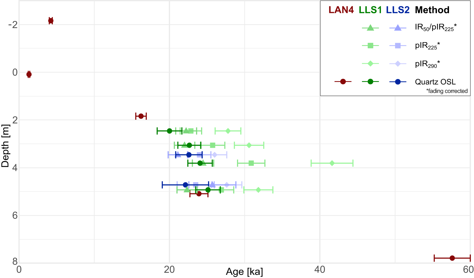
Detailed results from the luminescence dating are presented in Table 1 and visualised in Figure 5. Quartz OSL from LAN 4, arranged from the uppermost to the lowermost stratigraphic position, dates to 4.2 ± 0.2 ka, 1.3 ± 0.1 ka, 16.2 ± 0.7 ka, 23.9 ± 1.2 ka, and 57.6 ± 2.4 ka. At profile LLS 1, the quartz OSL ages increase slightly from 20.0 ± 1.7 ka at layer LLS 1-f to a maximum of 24.05 ± 1.62 ka for layer LLS 1-o. At LLS 2, the quartz OSL ages are indistinguishable at 25.11 ± 1.64 ka and 22.57 ± 1.76 ka for layers LLS 2-e and LLS 2-i. The polymineral ages measured from LLS 1 and LLS 2 tend to overestimate the quartz ages, but fading-corrected IR50 and pIRIR225 are often within 1 SD of uncertainty of the quartz ages for the individual samples.
Luminescence age results with 1 SE from the loess–palaeosol sequences (LPS) LLS 1 and LLS 2 and sediment core LAN 4. Note that for LAN 4, the depth was plotted as 0 m at the top of the buried Holocene chernozem to better align with the depth to LLS 1 and LLS 2. OSL, optically stimulated luminescence; pIRIR, post–infrared-stimulated luminescence–infrared-stimulated luminescence.

Figure 5 Long description
The plot shows luminescence age results versus depth for sequences LAN4, LLS1 and LLS2. The x-axis is labeled ′Age′ in kiloannum (ka), ranging from 0 to 60. The y-axis is labeled ′Depth′ in meters, with depth increasing downward. Data points represent different luminescence methods indicated by different symbols: IR subscript 50 slash pIR subscript 225, pIR subscript 225, pIR subscript 290 and Quartz OSL, with fading correction noted for all but quartz. LAN4 data points are shown in red, LLS1 in green and LLS2 in blue. Error bars indicate one standard error for each measurement. All precise positions and age results are also given in numbers in Table 1.
Data relating to dose rate calculation, burial dose determination and the resulting ages for each sample from the LPS LLS 1 and LLS 2 and sediment core LAN 4 (uncertainties represent 1 SE).

Table 1 Long description
The table reports luminescence dating inputs and results for multiple sediment samples, including radionuclide concentrations, water content, dose rates, burial doses, and calculated ages with one standard error. For the LAN4 core measured with quartz OSL, ages, except for the uppermost one, increase strongly with depth: about 4.2 ka at 1.25 m, 1.3 ka at 3.5 m, 16.2 ka at 5.25 m, 23.9 ka at 8.5 m, and 57.6 ka at 11.2 m, while dose rates stay fairly similar at roughly 3.4 to 3.8 Gy per thousand years. LLS1 quartz OSL ages cluster in the late Pleistocene, about 20.0 ka at 2.47 m, 22.6 ka at 3.07 m, 24.1 ka at 3.82 m, and 25.1 ka at 4.94 m, with dose rates around 3.4 to 3.8 Gy per thousand years. LLS2 quartz OSL ages are about 22.6 ka at 3.47 m and 22.1 ka at 4.73 m, despite higher scatter for the deeper LLS2 sample. Overdispersion is generally low in LAN4 (about 0 to 8 percent) but can be higher in LLS samples, reaching about 25 percent in LLS2-i, indicating more spread among aliquots. Several LLS samples also include feldspar post-IR IR protocols that report g-values and corrected ages; these corrected ages are broadly similar to the quartz ages. Comparisons across protocols should be made cautiously because different minerals and fading corrections can affect the final ages.
a Stratigraphic unit: corresponds to the stratigraphic unit assigned in Fig. 4 from which the sample was taken.
b Protocol: luminescence measurement protocol applied to each sample, as described in the “Material and Methods” section.
c OD, overdispersion.
Discussion
Multiproxy data for profile synthesis
Influences of slope processes at LLS 1 and LLS 2 from grain-size signals
The elevated sand contents in LLS 1 and LLS 2 show two distinct signals from the fine sand and the medium to coarse sand fractions, indicating a polygenetic signature of aeolian and primary slope processes. The medium sand sub-modes (>400 μm) and the systematic presence of sandy bands are characteristic of sheetwash and solifluction, as observed at the nearby site of Krems-Wachtberg (Sprafke et al., Reference Sprafke, Schulte, Meyer-Heintze, Händel, Einwögerer, Simon, Peticzka, Schäfer, Lehmkuhl and Terhorst2020). Because primary loess is typically devoid of grains in the upper medium sand range (Pye, Reference Pye1995; Vandenberghe, Reference Vandenberghe2013), these coarser particles require a non-aeolian local source. We therefore infer the presence of a fluvial terrace outcrop or shallow exposure between LAN 4 and LLS 1. Coarse terrace material was likely redistributed downslope and incorporated into the loess matrix at the footslope positions.
The increase in the finer sand fraction (<400 μm) could result from selective hydraulic sorting of loessic grains during downslope redistribution or from short-distance aeolian transport from the Kamp River floodplain. Due to the proximity and lower elevation of LLS 1 and LLS 2 relative to the fluvial source, these profiles received higher aeolian sand inputs compared with the more distant and topographically higher LAN 4. A denser vegetation cover at the foot of the slope, closer to the river, could have trapped both aeolian and reworked sand (cf. Bosq et al., Reference Bosq, Bertran, Degeai, Kreutzer, Queffelec, Moine and Morin2018). Hence, the origin of the finer sand fractions may result from either or both aeolian sand input and reworked loess.
Given that slope processes repeatedly overprinted LLS 1 and LLS 2, any interpretation of aeolian dynamics based on the GSI must be used with caution (Schulte et al., Reference Schulte, Sprafke, Rodrigues and Fitzsimmons2018; Sprafke et al., Reference Sprafke, Schulte, Meyer-Heintze, Händel, Einwögerer, Simon, Peticzka, Schäfer, Lehmkuhl and Terhorst2020). Sheetwash mobilises the coarse silt and sand fractions better than the more cohesive finer fractions (Vandenberghe et al., Reference Vandenberghe, Sun, Wang, Abels and Liu2018; Zhang et al., Reference Zhang, Ma, Liu, Lei, Liu and Du2022). Therefore, sheetwash leads to higher GSI values, so the GSI at active slope locations reflects both wind dynamics and slope stability. To distinguish between these signals in our slope LPS, we include sand content, modal grain size, and colour in our assessment, and generally treat the GSI with caution.
We propose that, for a stand-alone index of wind dynamics in settings not purely of aeolian genesis, the most reliable indicator of changing wind dynamics is the modal grain size, as the modal position is mostly unaffected by the addition of coarse particles from slope processes (Vandenberghe et al., Reference Vandenberghe, Sun, Wang, Abels and Liu2018). This also holds true for loess that has been subject to strong pedogenic processes, as increasing clay mineral formation could hardly exceed the modal volume in the coarse silt fraction.
Geochemical and colour signals in a carbonate-rich loess context
A strong correlation between L* and carbonate content indicates that brightness in these sequences serves as a proxy for loessification (calcification) rather than for organic matter content. This is especially true because the measured organic carbon content was too low to reliably detect any variations within the measurement accuracy.
Carbonate contents are very high throughout all LPS, reaching about 35 wt% at the top of LAN 4 and decreasing to roughly 20 wt% in the lower parts of LLS 1 and LAN 4. Comparable high carbonate contents in upper pleniglacial loess have been documented in nearby LPS (Gocke et al., Reference Gocke, Hambach, Eckmeier, Schwark, Zöller, Fuchs, Löscher and Wiesenberg2014; Krauß et al., Reference Krauß, Zens, Zeeden, Schulte, Eckmeier and Lehmkuhl2016; Meyer-Heintze et al., Reference Meyer-Heintze, Sprafke, Schulte, Terhorst, Lomax, Fuchs and Lehmkuhl2018; Sprafke et al., Reference Sprafke, Schulte, Meyer-Heintze, Händel, Einwögerer, Simon, Peticzka, Schäfer, Lehmkuhl and Terhorst2020). Under such alkaline conditions, leaching is weak, and silicate alteration remains limited, especially in the younger parts of the sequences.
In this setting, the CIA largely reflects carbonate variability rather than isolating silicate weathering. For the CIA to reliably reflect silicate weathering rather than contributions from easily dissolved carbonates or phosphates, a correction for the measured CaO is required (Nesbitt and Young, Reference Nesbitt and Young1982; McLennan, Reference McLennan1993; Buggle et al., Reference Buggle, Glaser, Hambach, Gerasimenko and Marković2011; Schatz et al., Reference Schatz, Scholten and Kühn2014). Applying a CaO* correction following McLennan (Reference McLennan1993) effectively substitutes silicate CaO by Na2O at these LPS, which makes CIA behaviour converge toward that of CPA. Compared with the CIA, the CPA shows broadly similar changes, but with smaller amplitudes and higher background variability. Due to the very weak pedogenic alteration of silicates, the general background noise, caused by minor heterogeneities in the material and the method, is significant (Yang et al., Reference Yang, Li, Yang and Li2004; Buggle et al., Reference Buggle, Glaser, Hambach, Gerasimenko and Marković2011). We therefore interpret CIA and CPA only in conjunction with other colour and clay-related proxies and do not infer pedogenesis from small excursions in these indices.
Colour as the most sensitive index for initial pedological processes
Colour is often more sensitive than ΔGSDclr to the earliest stages of pedogenesis under an alkaline buffer (Ji et al., Reference Ji, Balsam, Chen and Liu2002; Buggle et al., Reference Buggle, Hambach, Müller, Zöller, Marković and Glaser2014; Sprafke et al., Reference Sprafke, Schulte, Meyer-Heintze, Händel, Einwögerer, Simon, Peticzka, Schäfer, Lehmkuhl and Terhorst2020). In the LPS, intervals with higher a* do not systematically coincide in places with modest CIA or CPA increases and elevated ΔGSDclr, which would be consistent with weak oxidation and initial clay formation. Two brownish CB horizons, LLS 1-k and LAN 4-r, show clear ΔGSDclr signals, but other brownish units lack such a response and display only faint changes in geochemical indices. In such intervals, iron oxide pigments can be adsorbed to the surface of silt and sand particles, while clay aggregates are mobilised by sheetwash or solifluction, producing brown hues without a clay signal. Therefore, we interpret brownish horizons as pedogenic only when colour, ΔGSDclr, and geochemistry converge. Otherwise, we interpret them as reworked slope material.
Proxy signals of reduction features and solifluction
Horizons with reduction features exhibit lower b* values, but rarely show consistent responses in other proxies. In these units, ΔGSDclr shows no significant peaks; CIA and CPA exhibit only small, irregular minima; and clay and sand contents fluctuate without a stable pattern. We interpret these horizons with reduction features as tundra gley horizons formed under seasonal waterlogging above permafrost, consistent with established observations from European loess records (Antoine et al., Reference Antoine, Rousseau, Moine, Kunesch, Hatté, Lang, Tissoux and Zöller2009b; Terhorst et al., Reference Terhorst, Sedov, Sprafke, Peticzka, Meyer-Heintze, Kühn and Solleiro Rebolledo2015; Sprafke et al., Reference Sprafke, Schulte, Meyer-Heintze, Händel, Einwögerer, Simon, Peticzka, Schäfer, Lehmkuhl and Terhorst2020). Under such conditions, iron is reduced, producing grey to bluish hues, while the alkaline carbonate buffer limits hydrolysis and clay neoformation. Local capillary enrichment of CaCO3 can accompany reduction, as observed in nearby sequences (Cilek, Reference Cilek2001; Meyer-Heintze et al., Reference Meyer-Heintze, Sprafke, Schulte, Terhorst, Lomax, Fuchs and Lehmkuhl2018), further explaining the weak CIA and CPA signals.
The increased sand contents in the Cr horizons can be the result of reducing conditions overprinting previously reworked material or solifluction during Cr formation and degradation. The high water saturation required to reduce oxides may also indicate high pore pressures, which tend to trigger soil movement on slopes (Kemp, Reference Kemp2001), leading to the reworking of the deposited loess and the mixing with coarser sediments from upslope sites. Seasonal thawing of the active layer and snowmelt during interstadials could have contributed to this, as the resulting surface runoff selectively transports particles by size (Asadi et al., Reference Asadi, Moussavi, Ghadiri and Rose2011). LAN 4-w, the most developed reduction horizon, most likely reflects these conditions, as it coincides with a shift to a coarser modal grain size and a higher modal concentration, resulting from slope processes preferentially mobilising non-cohesive coarse material over cohesive fines (Vandenberghe et al., Reference Vandenberghe, Sun, Wang, Abels and Liu2018; Zhang et al., Reference Zhang, Ma, Liu, Lei, Liu and Du2022). Although this layer appears not to have developed conclusively in situ, it indicates environmental conditions similar to those of Cr, without signs of reworking.
Chronology
As the quartz luminescence signal is not affected by fading, and all our quartz samples show adequate luminescence properties with none reaching saturation, we selected quartz-based ages to establish the chronologies of our three records. Silt-sized quartz grains were used to target the dominant grain-size fraction of loess. Another advantage of silt-sized grains for dating is higher precision of associated luminescence ages due to stronger signals compared with aliquots based on sand-sized grains. The disadvantage of silt dating, on the other hand, is its limited efficiency in detecting incomplete signal resetting. For sediments affected by slope transport, dating of sand grains might provide more accurate ages.
We investigated this at the LLS 1 and LLS 2 outcrops, as their positions are affected by steeper slopes, and the elevated sand fraction content could lead to a larger proportion of poorly bleached, non-aeolian grains. For all but sample C-L5108, the fine-grained fraction does not appear to be affected by incomplete bleaching. Despite the IR50 and pIRIR signals being bleached by sunlight at significantly slower rates compared with quartz (e.g., Buylaert et al., Reference Buylaert, Jain, Murray, Thomsen, Thiel and Sohbati2012), the age difference between quartz and polymineralic luminescence ages at the LLS outcrops is relatively small or indistinguishable within dating uncertainties (cf. Murray et al., Reference Murray, Thomsen, Masuda, Buylaert and Jain2012). Fine-grain quartz ages are, thus, assumed to provide a robust chronology for the majority of the dated samples. The only exception is sample C-L5108 (LLS 1-o), where fading-corrected pIRIR225 (30.9 ± 1.8 ka) and pIRIR290 (41.6 ± 2.8 ka) ages appear significantly older than the associated quartz age (24.1 ± 1.6 ka). Here, we cannot exclude age overestimation, but quartz must also be assumed to provide the best age estimate. Therefore, we only consider quartz OSL ages for all further chronological interpretation.
After inspection of the multiproxy data, it turned out that three of the OSL samples in LAN 4 were not taken from the LPS. The oldest age sample originated from fluvial terrace sediments (C-L5229), and the two uppermost luminescence samples were found to belong to anthropogenically displaced sediment due to terracing and ploughing during viticulture (C-L5225 and C-L5226).
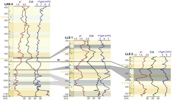
Correlation between loess–palaeosol sequences (LPS) LLS 1 and LLS 2 and sediment core LAN 4 in Langenlois. Tie point (TP) connecting the three LPS. Other lines showing corresponding times across the LPS are based on sediment properties and stratigraphy similarities, rendering them less definitive. CIA, Chemical Index of Alteration.

Figure 6 Long description
Three stratigraphic logs are displayed side by side for sediment sections LAN 4, LLS 1 and LLS 2. Each log shares a common structure: the vertical axis represents depth in centimeters and three curves are plotted horizontally against that depth. The three horizontal variables plotted in each log are a* (the CIELAB redness parameter), Chemical Index of Alteration (CIA) and volume percent of particles smaller 1 µm (<1µm) . Each log contains alternating shaded horizontal bands representing distinct stratigraphic units. Stratigraphic layers are labeled alphabetically from a downward in each log. A tie point labeled TP connects LAN 4 at approximately 855 centimeters to LLS 1 at approximately 300 centimeters and to LLS 2 at approximately 360 centimeters. Additional correlation connectors link corresponding horizons across the three logs at multiple depths, based on matching patterns across all indices. . Quartz optically stimulated luminescence dates are marked at specific depths; for the results, see Table 1 and Figure 5.
Interprofile correlations at Langenlois of LAN 4, LLS 1, and LLS 2
As the pedogenic signals are all very weak and LLS 1 and LLS 2 have been subject to repeated slope processes, identifying horizons in all three LPS that formed simultaneously is difficult. The closest to unaltered loess layers are LAN 4-m, LLS 1-g, and LLS 2-e, characterised by the lowest values for chemical weathering-related indices (especially the CIA), the highest grain concentration in the modal grain-size class, and a bright-yellowish colour. The shared proxy signature, similar stratigraphic context, and overlapping quartz OSL ages strongly suggest synchronous formation. We therefore use these horizons as tie points for the intra-site correlation (Fig. 6). From this point onward, the correlation is based on the weakly developed Cryosols, as they are most likely to have formed in situ.
LLS 1 and LAN 4 show a distinct transition between the lower and upper sediments across several proxies, with more intense pedological processes in the lower parts. In LLS 2, the transition is not clearly identifiable, as the LPS is shorter and underwent more reworking than the others. This transition is not abrupt but extends over several layers, with the upper boundaries coinciding with the tie points, allowing precise dating of the completed transition to a pedologically less active time at about 24 ka. In the lower parts, more intense chemical weathering occurred, as shown by increased CIA values and CaCO3 leaching, likely contributing to its generally darker colour and increased clay content. Together, this information suggests a warmer and more humid climate that facilitated more intense pedogenesis. This internal transition accords with regional evidence for increasing aridity and wind strength around 23 ka (Antoine et al., Reference Antoine, Rousseau, Degeai, Moine, Lagroix, Kreutzer and Fuchs2013, Reference Antoine, Coutard, Guerin, Deschodt, Goval, Locht and Paris2016; Meszner et al., Reference Meszner, Kreutzer, Fuchs and Faust2013; Fitzsimmons and Hambach, Reference Fitzsimmons and Hambach2014; Moine et al., Reference Moine, Rousseau and Antoine2008, Reference Moine, Antoine, Hatté, Landais, Mathieu, Prud’homme and Rousseau2017), marking the shift from Upper Pleniglacial A to B in European loess (Lehmkuhl et al., Reference Lehmkuhl, Zens, Krauß, Schulte and Kels2016) and corresponding to a change from tundra to polar desert in the ELSA Landscape Evolution Zones (Sirocko et al., Reference Sirocko, Knapp, Dreher, Förster, Albert, Brunck and Veres2016; Fig. 7). Weakly developed Cryosols immediately above the transition in LLS 1 and LAN 4 occur within the time window of Greenland Interstadial 2, dated at 23.34–23.22 ka (GI-2.2; Rasmussen et al., Reference Rasmussen, Bigler, Blockley, Blunier, Buchardt, Clausen and Cvijanovic2014).
Correlating loess–palaeosol sequence (LPS) LAN 4 based on optically stimulated luminescence (OSL) dates and multiple indices with dust concentration (Ruth et al., Reference Ruth, Bigler, Röthlisberger, Siggaard-Andersen, Kipfstuhl, Goto-Azuma, Hansson, Johnsen, Lu and Steffensen2007) and oxygen isotope data (NGRIP; North Greenland Ice Core Project Members, 2007) and Greenland interstadials (GI) (Rasmussen et al., Reference Rasmussen, Bigler, Blockley, Blunier, Buchardt, Clausen and Cvijanovic2014) from NGRIP, Simplified General Loess Stratigraphy Germany (Lehmkuhl et al., Reference Lehmkuhl, Zens, Krauß, Schulte and Kels2016; Zens et al., Reference Zens, Zeeden, Römer, Fuchs, Klasen and Lehmkuhl2017), and the LPS at Krems-Wachtberg (KW2015-A 2015) (Sprafke et al., Reference Sprafke, Schulte, Meyer-Heintze, Händel, Einwögerer, Simon, Peticzka, Schäfer, Lehmkuhl and Terhorst2020). CIA, Chemical Index of Alteration.

Figure 7 Long description
The figure correlates Greenland NGRIP climate proxies (dust, δ18O), the Simplified General Loess Stratigraphy Germany and the loess stratigraphy of Krems Wachtberg A (KW-A) with the loess stratigraphy of LAN 4. The first panel shows Simplified General Loess Stratigraphy with age in ka, highlighting transitions between Upper Pleniglacial A and B and Holocene. The second panel, NGRIP, plots dust concentration in microgram per kilogram against age. The third panel, NGRIP, displays delta 18 O H2O in per mil SMOW against age, with lower values corresponding to higher dust intervals. Red numbers 2, 3 and 4 mark Greenland interstadials (GI). The fourth panel, LAN 4, shows three horizontally plotted variables a* (the CIELAB redness parameter), Chemical Index of Alteration (CIA) and volume percent of particles smaller 1 µm (<1µm) against depth in centimeters. Key transitions occur around 16.2 ka and 22.5 ka, indicating shifts in pedogenesis and climate conditions. The fifth panel, KW-A, also plots depth with the same variables as LAN 4, showing distinct stratigraphic layers and changes across all indices. Overall, the figure highlights correlations between climate proxies and loess stratigraphy, with major transitions marked by changes in dust, delta 18 O and other indices.
In the uppermost layers, LLS 1-c/b/a, the modal grain size shifts by up to two grain-size classes toward coarser grains, similar to the shift above LAN 4-j. In LLS 2, a similar shift occurs throughout LLS 2-h/g/f. However, given the established correlation, this cannot be matched to the other two LPS. These shifts in modal grain size may be due to changes in aeolian dynamics, the availability or instability of the source material, or slope stability. However, it is not possible to determine the exact process responsible.
LLS 2 contains multiple layers (LLS 2-i/f/d) with GSDs skewed toward the medium sand fraction, indicative of disturbance in the loess. Given the notably high GSI values, low weathering indices, and no signs of reducing conditions around the layers, this suggests a barren, open landscape prone to erosion by wash and other slope processes. These anomalies in the medium sand fraction are unique to LLS 2 and are not observed in LLS 1, pointing toward a localised signal driven by microtopographic control. We infer a palaeo-depression at the LLS 2 position that focused reworking and rapid infill, producing systematic medium sand anomalies and weaker pedogenic imprints due to higher sedimentation rates (Muhs and Bettis, Reference Muhs and Bettis2003; Rousseau et al., Reference Rousseau, Boers, Sima, Svensson, Bigler, Lagroix, Taylor and Antoine2017; Fischer et al., Reference Fischer, Hambach, Klasen, Schulte, Zeeden, Steininger, Lehmkuhl, Gerlach and Radtke2019). This also explains the disruption of the reduction layers (LLS 2-h/f) by a slightly brownish, probably reworked material.
Profile LAN 4, with its stable plateau position, provides a continuous in situ record that is less susceptible to slope-induced reworking than the brickyard profiles, making it the most robust candidate for inter-archive correlation. It represents a wider record of the LGM loess. However, the lower parts of LAN 4 are likely to have experienced some erosion, so they should be approached with caution.
Correlation to other archives
LAN 4 extends down into the terrace. The first loess layer above the terrace gravels (LAN 4-zz) shows a strong increase in clay content, from ∼6 to ∼9 vol% (a relative increase of ∼50%), compared with the overlying sections, representing the highest clay content observed within the profile. The ΔGSDclr, indicative of postdepositional clay formation, shows a similar increase. However, a minor sub-mode within the upper medium sand fraction, consistent with a minor admixture of terrace materials, suggests that this layer may have been reworked. Below the loess, the terrace gravels are draped with finer materials, yielding a quartz OSL age of 57.6 ± 2.4 ka and differing markedly from overlying loess across all proxies. The high clay content is consistent with deposition of upstream-derived fine alluvial sediments during flooding and a low-energy setting during cold–warm transitions (Vandenberghe, Reference Vandenberghe2015). A similar gravel–sandy–loamy clayey sequence has been described at the nearby Hammerer brickyard (Piffl, Reference Piffl and Fink1976), and comparable shallow-water drapes on terrace tops are widely reported in the region.
The age gap between the basal terrace fines and the overlying loess across a short stratigraphic interval implies a hiatus. The abrupt transition at LAN 4-z/zz likely marks a local unconformity. However, the entire section from LAN 4-q to LAN 4-z shows many abrupt changes, which may also result from eroded sediments. Such discontinuities are documented at Langenlois and Stratzing, where late MIS 3 loess is missing (Thiel et al., Reference Thiel, Terhorst, Jaburová, Buylaert, Murray, Fladerer, Damm, Frechen and Ottner2011a, Reference Thiel, Buylaert, Murray, Terhorst, Hofer, Tsukamoto and Frechen2011b).
To establish a local correlation, we cautiously compare LAN 4 with the well-studied LPS at Krams-Wachtberg (KW2015-A; Sprafke et al., Reference Sprafke, Schulte, Meyer-Heintze, Händel, Einwögerer, Simon, Peticzka, Schäfer, Lehmkuhl and Terhorst2020), only 6 km away. Similar to LLS 1 and LLS 2, KW2015-A shows repeated reworking across large parts of the last glacial loess, complicating its correlation with LAN 4. The whole section from LAN 4-q to LAN 4-z has strong similarities to sections V and IV of the LPS at KW2015-A, fitting the sequence and helping to establish an absolute time frame (Fig. 7). The C/CB/BC layers at around 2 m depth in KW2015-A are much thicker than in LAN 4-p. However, in KW2015-A, these layers were identified as subject to reworking, possibly increasing total sedimentation by admixing materials from upslope, whereas LAN 4-p shows no signs of reworking.
A cautious alignment correlates the uppermost Cr in KW2015-A with LAN 4-e. Relative stratigraphy places their formation at around 20 ka, further supported by slowly decreasing sedimentation rates and its placement between the OSL dates. Above the KW2015-A LPS ends, while LAN 4 provides ∼2 m of loess sediments, showcasing a faint Cr in LAN 4-b, beginning 60 cm below the upper end of the LPS, dated to 16.2 ± 0.7 ka.
As observed in KW2015-A and other sites in lower Austria, late last glacial loess is often discontinuous or truncated (Thiel et al., Reference Thiel, Terhorst, Jaburová, Buylaert, Murray, Fladerer, Damm, Frechen and Ottner2011a, Reference Thiel, Buylaert, Murray, Terhorst, Tsukamoto, Frechen and Sprafke2011c). Within the regional context of lower Austria, these ages only correlate with the loess unit overlying the upper Cryosol at Joching, which yielded a comparable age of 16 ± 2 ka (Thiel et al., Reference Thiel, Buylaert, Murray, Terhorst, Tsukamoto, Frechen and Sprafke2011c). Against this background, the preservation of young loess in the upper part of LAN 4 provides a valuable local archive for the late last glacial. Under polar desert conditions, pedogenesis was very limited, while dust accumulation remained substantial at many sites, so upper units typically display only minor stratigraphic variability.
The regional reference site, Krems-Wachtberg (Terhorst et al., Reference Terhorst, Kühn, Damm, Hambach, Meyer-Heintze and Sedov2014; Sprafke et al., Reference Sprafke, Schulte, Meyer-Heintze, Händel, Einwögerer, Simon, Peticzka, Schäfer, Lehmkuhl and Terhorst2020), has been successfully correlated with Greenland ice-core records (NGRIP; North Greenland Ice Core Project Members, 2007), indicating that the North Atlantic atmospheric circulation influenced the palaeoclimatic regime in the studied region. We correlated periods of high dust concentration in NGRIP with increased loess accumulation, a coarser modal grain size due to stronger winds and minimal pedogenic activity in Langenlois. Similarly, higher δ18O values and lower dust concentrations in NGRIP align with Cryosol formation phases in LAN 4 (Fig. 7). Following this, GI 2 can be correlated with the Cr horizon in LAN 4-l, and GI 3 with LAN 4-w. The interval following GI 2 is characterised by high sedimentation rates with only faint pedogenic signals in LAN 4 and minor fluctuations in NGRIP. Based on relative stratigraphic positioning and comparison with the KW2015-A sequence and general German loess stratigraphy, unit LAN 4-e is tentatively assigned a formation age of approximately 20 ka BP. However, direct chronometric confirmation for this specific unit is currently absent. Furthermore, the small fluctuations preclude a precise correlation of the uppermost faint Cr horizon in LAN 4-b with specific NGRIP events.
Conclusions
Located at the climatic transition between the humid Atlantic west and drier continental east, Langenlois’s LPS are susceptible to small shifts in temperature and moisture on an intrastadial/interstadial scale during MIS 2. The records reveal alternations between aeolian loess accumulation under cold, arid conditions, and weak, short-lived Cryosol formation during brief interstadial periods. In this threshold environment, slight warming can initiate incipient pedogenic processes but stop just as fast when conditions revert. Consequently, while the archive responds sensitively, it predominantly records subtle, easily overprinted signals.
Our results demonstrate that robust interpretation of weakly differentiated, carbonate-rich LPS requires both a multiproxy and a multi-profile perspective along a slope gradient. Single proxies are insufficient when pedogenesis is incipient, carbonate buffers geochemical signals, and local geomorphodynamics rework and alter aeolian deposits. Although field descriptions are an important aspect of deciphering LPS, in these poorly developed LPS, they provide only minor interpretive value, because the various layers and features are hardly distinguishable in the field. Coherent inferences emerge only when colour, ΔGSDclr, modal grain size, sand content, and weathering indices are evaluated together, and when LPS along a slope transect are compared to separate local from regional signals.
However, the considerable inter-profile variability only allows for a conservative correlation. The combination of OSL dates and stratigraphic sequence enabled a single tie point to be identified with sufficient confidence to serve as a basis for further cautious correlation.
On the lower slope, both LLS 1 and LLS 2 record repeated overprinting by slope processes. Persistent sandy bands, medium sand sub-modes, and poorer sorting indicate sheetwash and solifluction as recurrent controls, with LLS 2 most strongly affected. By contrast, the higher, gentler slope position at LAN 4 preserves a more typical loess GSD and retains young loess that is frequently truncated elsewhere in the region, with quartz OSL ages indicating deposition at least until 16.2 ± 0.7 ka. The basal contact shows fine loess draped over terrace gravels and a short interval to overlying MIS 2 loess, indicating a local hiatus at the MIS 3/2 boundary that is common in the region.
A weak but discernible signal of GI-2 is present in Langenlois LPS LAN 4 and LLS 1. More notably, the LPS record a clear transition from tundra to polar desert environments, completed around 24 ka BP. There are also additional fluctuations that can be cautiously correlated with smaller climate fluctuations recorded in NGRIP. However, linking these more robustly would require further dating. This highlights the high sensitivity of the Langenlois LPS to climate fluctuations during MIS 2, although this sensitivity results in signals that are only weakly developed. Nevertheless, we have demonstrated that by combining multiple closely situated LPS and employing a variety of proxies, these signals can be detected and differentiated.
Supplementary material
The supplementary material for this article can be found at https://doi.org/10.1017/qua.2026.10097.
Acknowledgments
The fieldwork and laboratory analyses were funded by the Deutsche Forschungsgemeinschaft (DFG, German Research Foundation)—project no. 57444011–SFB 806 “Our Way to Europe.” We thank our colleagues for help with geophysical measurements (Florian Steiniger), during fieldwork (Ulrich Hambach, Thomas Einwögerer, Stephan Pötter, Bernhard Pröschel, Svenja Püschel), and with creating the maps (Johannes Souren). We express our particular gratitude to Tobias Sprafke for his assistance in interpreting the LPS and extracting the stratigraphies. We also want to express our appreciation to the two reviewers who provided valuable, constructive feedback on an earlier version of the article.