What is already known?

The I-squared statistic has enjoyed considerable success in meta-analysis. It has recently been stated that, informally, I-squared can be considered to reflect the extent to which confidence intervals displayed in a forest plot do not overlap with each other.

What is new?

We investigate mathematically how I-squared is calibrated to the extent to which confidence intervals do, and do not, overlap. By doing so, we are able to formalise this interpretation of I-squared.

Potential impact for RSM readers

Readers may not be aware of this particular interpretation of I-squared. Our work opens up possibilities, based on forest plots and confidence interval overlap, for measuring inconsistencies in trial results in meta-analysis.

2.1. The probability that confidence intervals in a forest plot overlap

Consider, without loss of generality, the first two study estimates under the random-effects model,Reference Higgins, Thompson and Spiegelhalter ^{8 ,} Reference DerSimonian and Laird ⁹ $Y_1 \sim N(\mu , \sigma ^2+\tau ^2)$ and $Y_2\sim N(\mu , \sigma ^2+\tau ^2)$ . Assuming that the within-study variances are known without error, the corresponding 95% confidence intervals, displayed on a forest plot, are given by $(Y_1 - 1.96\sigma , Y_1 + 1.96\sigma )$ and $(Y_2 - 1.96\sigma , Y_2 + 1.96\sigma )$ . If $-2\times 1.96\sigma < Y_2 - Y_1 < 2\times 1.96\sigma ,$ then their 95% confidence intervals overlap. This is because these confidence intervals extend $1.96\sigma $ in each direction from $Y_1$ and $Y_2$ , so that we have overlap if the absolute difference between the point estimates is less than $2\times 1.96\sigma $ . Let us define $D=Y_2 - Y_1 \sim N(0, 2(\sigma ^2+\tau ^2))$ . Then the probability that the 95% confidence intervals in a forest plot overlap, $P(\text {overlap})$ , is

$$\begin{align*}P(\text{overlap}) = P(-2\times1.96\sigma < D<2\times1.96\sigma). \end{align*}$$

Defining $Z=D/\sqrt {2(\sigma ^2+\tau ^2)} \sim N(0,1)$ , we can write this as

$$\begin{align*}P(\text{overlap}) = P \left(- \sqrt{2}\times1.96\sqrt{\frac{\sigma^2}{\sigma^2+\tau^2}} < Z < \sqrt{2}\times1.96\sqrt{\frac{\sigma^2}{\sigma^2+\tau^2}}\right). \end{align*}$$

Then, from the definition of $I^2$ in equation (1),

$$\begin{align*}P(\text{overlap}) = P \left(- \sqrt{2}\times1.96\sqrt{1-I^2} < Z < \sqrt{2}\times1.96\sqrt{1-I^2}\right). \end{align*}$$

Noting that Z is standard normal, this is

$$\begin{align*}P(\text{overlap}) = \Phi(\sqrt{2}\times1.96\sqrt{1-I^2}) - \Phi(-\sqrt{2}\times1.96\sqrt{1-I^2}), \end{align*}$$

where $\Phi (\cdot )$ is the standard normal cumulative distribution function. The key function is $f(I^2) = \sqrt {2}\times 1.96\sqrt {1-I^2}$ . Using this definition, we have

$$\begin{align*}P(\text{overlap}) = \Phi(f(I^2)) - \Phi(-f(I^2)). \end{align*}$$

There are many equivalent ways to write this quantity but we cannot make further analytical progress. From the symmetry of the normal distribution, $\Phi (-x) = 1- \Phi (x)$ , we can write this as

(2) $$ \begin{align} P(\text{overlap}) = 2\Phi(f(I^2)) -1. \end{align} $$

There are $n(n-1)/2$ pairs of confidence intervals, where n is the number of studies. Therefore, the expected number of pairs of confidence intervals that overlap on a forest plot, $E(\text {overlap})$ is

(3) $$ \begin{align} E(\text{overlap}) = \frac{n(n-1)}{2}P(\text{overlap}). \end{align} $$

If $I^2=1/2,$ then $f(I^2)=1.96$ , so that $P(\text {overlap}) = 2\Phi (1.96) -1 = 0.95$ . Hence, if $I^2=1/2$ , then the probability of confidence interval overlap is equal to the coverage probability of the confidence intervals. The function $f(I^2)$ is decreasing in $I^2$ , and $P(\text {overlap})$ in equation (2) is increasing in $f(I^2)$ , so that $P(\text {overlap})$ is decreasing in $I^2$ . This investigation therefore formalises the statement made by Higgins and López-LópezReference Higgins and López-López ³ that $I^2$ can be considered to reflect the extent to which confidence intervals displayed in a forest plot do not overlap with each other. Equation (2) describes this intuition in simple and direct mathematical form.

2.2. The probability that confidence intervals in a forest plot do not overlap

Higgins and López-LópezReference Higgins and López-López ³ focus on $I^2$ as reflecting the extent to which confidence intervals displayed in a forest plot do not overlap with each other. We have instead derived results for the probability that these confidence intervals do overlap. We have done this because this simplifies the presentation of our mathematical derivations; we can then evaluate the probability that a normally distributed random variable lies within one interval of finite length ( $-2\times 1.96\sigma < D<2\times 1.96\sigma $ ), instead of two intervals of infinite length ( $D> 2\times 1.96\sigma $ or $D< -2\times 1.96\sigma $ ). This becomes more useful in Section 2.5 where we calculate the probability that a bivariate normal random variable lies within a finite square, centred at the origin. However, all our results are easily communicated in terms of $P(\text {not overlap})$ , which is simply the complement of equation (2). Furthermore, in Section 2.5, we can easily derive the mean and variance of $1-O$ , which is the proportion of confidence intervals that do not overlap.

2.3. Other straightforward extensions

Critical values other than $k=1.96$ could also be considered, where natural choices are $k=1$ and $k=0.675$ . The former value uses error bars of one standard deviation and the latter corresponds to confidence interval coverage of 1/2, so that these two values capture typical variation in two different senses. Alternatively, critical values corresponding to other significance levels could also be used. If an alternative value to $k=1.96$ is used, then the key function becomes $f(I^2, k) = \sqrt {2}\times k \sqrt {1-I^2}$ and all formulae then apply with this new function. If $k=1.96,$ then all results simplify to those given previously, so that $f(I^2, 1.96) = f(I^2)$ . However, using alternatives to $k=1.96$ would require access to the meta-analytic dataset. This is because forest plots are rarely, if ever, presented using alternatives to 95% confidence intervals. This information may however be deducible in some instances from reported aggregate-level information. In practice, without this, it may in any case often be difficult to determine if confidence intervals in published forest plots overlap. This may need to be determined using high-level scans of these plots, and a keen eye or specialist software, unless these confidence intervals are also displayed numerically.

The above analysis required to compute $P(\text {overlap})$ in equation (2) is straightforward to generalise to the case where every study has different $\sigma _i^2$ . If desired, $E(\text {overlap})$ in equation (3) could then be computed by summing the ${n(n-1)}/{2}$ different values of study pair specific $P(\text {overlap})$ . However, the connection with $I^2$ would then be lost. The motivation for $I^2$ in any case rests on the assumption that a typical within-study variance is suitable. Hence, when investigating the implications of $I^2$ statistics mathematically, it is therefore probably most appropriate to consider the case where all studies have the same within-study variance, as we have here.

2.4. Numerical results

In Figure 1, we show the overlap probability (equation (2)) as a function of $I^2$ for three values of $k=0.675$ (green), $1$ (blue), and $1.96$ (black). We also show a vertical dotted line at $I^2=1/2$ and horizontal lines connecting the curves to the vertical axis at the overlap probabilities, at $I^2=1/2$ , of 1/2, $2\Phi (1)-1=0.683$ and 0.95, to aid interpretation. The probability that confidence intervals overlap is not very sensitive to the value of $I^2$ until this becomes larger than $1/2$ , but nevertheless the connections between $I^2$ and $P(\text {overlap})$ are clear.

Figure 1.

Probability of confidence interval overlap as a function of $I^2$ for $k=0.675$ (green), $k=1$ (blue), and $k=1.96$ (black). Dotted lines at $I^2=1/2$ and the corresponding confidence interval overlap probabilities are also shown to aid interpretation.

Figure 1 Long description

The x-axis is labeled I-squared and ranges from 0.0 to 1.0. The y-axis is labeled Overlap probability and ranges from 0.0 to 1.0. Three downward-sloping curves represent different k values.

* The top curve is black (k equals 1.96), starting near 1.0 probability at I-squared 0.0 and maintaining a high probability until dropping sharply after I-squared 0.8.

* The middle curve is blue (k equals 1), starting at approximately 0.85 probability and decreasing steadily.

* The bottom curve is green (k equals 0.675), starting at approximately 0.65 probability and decreasing steadily.

A vertical dashed line is positioned at I-squared equals 1/2 (0.5). Horizontal dashed lines extend from the y-axis to meet each curve at this vertical line.

* For the black curve, the intersection is at approximately 0.95 probability.

* For the blue curve, the intersection is at approximately 0.68 probability.

* For the green curve, the intersection is at 0.5 probability.

All three curves converge to 0.0 probability as I-squared reaches 1.0.

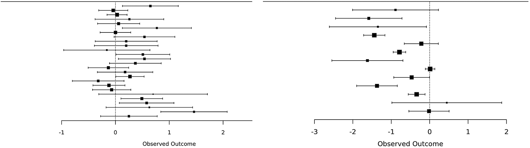
In Figure 2 (left), we show the essential elements of a conventional forest plot for an exampleReference Viechtbauer and Cheung ¹⁰ that has been used many times previously in methods work. Briefly, this example includes 26 studies exploring the effectiveness of writing-to-learn interventions. With 26 studies, there are $26\times 25/2 = 325$ pairs of confidence intervals that may, or may not, overlap. A standard random-effects meta-analysis, using the DerSimonian and Laird estimatorReference DerSimonian and Laird ⁹ of $\tau ^2$ , using the metafor packageReference Viechtbauer ¹¹ provided $I^2=55.9$ %. Metafor was also used to compute a 95% confidence interval for $I^2$ of (31.8%, 82.2%).

Figure 2.

Essential elements of forest plots examples exploring the effectiveness of writing-to-learn interventions (left) and the BCG vaccine against tuberculosis (right).

Figure 2 Long description

Two forest plots are displayed side-by-side.

Left Panel: Writing-to-learn interventions.

The x-axis is labeled Observed Outcome and ranges from -1 to 2. A vertical dashed line of no effect is positioned at 0. There are 20 individual data points represented by black squares of varying sizes, each with horizontal error bars representing confidence intervals. The majority of the data points are clustered between 0 and 1, indicating a positive effect. Several confidence intervals cross the zero line, while others remain entirely to the right of it. One outlier at the bottom shows a significantly higher positive outcome near 1.5.

Right Panel: B C G vaccine against tuberculosis.

The x-axis is labeled Observed Outcome and ranges from -3 to 2. A vertical dashed line of no effect is positioned at 0. There are 13 data points. The distribution is more spread out compared to the left panel. Most data points and their confidence intervals are located to the left of the zero line, ranging between -2 and 0, suggesting a protective effect. Two data points at the bottom have confidence intervals that cross the zero line, with one point estimate slightly above 0.

A computer program was written to enumerate the number, and proportion, of overlapping 95% confidence intervals in Figure 2 (left). This computed that $311/325=95.7$ % of the pairs of confidence intervals in Figure 2 (left) overlap. The majority of 95% confidence intervals therefore overlap, which might be thought to be contradictory to the quite large $I^2=55.9$ %. However, computing the overlap probability (equation (2)) with $I^2=55.9$ % gives 93.4%. Repeating this calculation with $I^2=31.8$ % and 82.2% gives 97.8% and 75.8%. Hence, the $I^2$ statistic for this example can be seen to be in good agreement with the proportion of overlapping confidence intervals (Figure 2, left).

In Figure 2 (right), we show the essential elements of a conventional forest plot for another familiar example. Briefly, this example includes 13 studies exploring the effectiveness of the BCG vaccine against tuberculosis and was taken from the metafor package.Reference Viechtbauer ¹¹ This example displays very considerable between-study variation. Analysis, conducted in the same way for the previous example, resulted in $I^2=92.1$ %, with 95% confidence interval (81.9%, 97.7%). Here, 55 of the 78 (70.5%) pairs of confidence intervals overlap. Computing the overlap probability (equation (2)) with $I^2=92.1$ % gives $56.4$ %. Repeating this calculation with $I^2=81.9$ % and 97.7% gives 76.2% and 32.6%. Hence, the $I^2$ statistic for this example can also be seen to be in agreement with the proportion of overlapping confidence intervals (Figure 2, right).

We have used two examples with notable between-study heterogeneity because, as noted above, the probability of confidence interval overlap is not sensitive to small values of $I^2$ (Figure 1). For examples with moderate or mild $I^2$ , for example, less than 30%, the vast majority of 95% confidence intervals will overlap. For examples such as these, analyses like the ones we have conducted would be much less interesting. This is because the conclusion that nearly all confidence intervals overlap, in agreement with the mild $I^2$ statistic, would be almost inevitable. In practice, our new results will be insightful for more heterogeneous datasets, such as the two we have explored here. The supplementary materials provide data, and R code, to produce all numerical results.

2.5. Further mathematical considerations

Although the above mathematical analysis requires only very elementary mathematical statistics, we would like to point out some subtle points for those who might consider extending this further. More generally, we might be interested in the properties of the random variable O, defined to be the proportion of confidence intervals in the forest plot that overlap. Let $N=n(n-1)/2$ be the number of pairs of confidence intervals in the forest plot, which may or may not overlap. Place the pairs of confidence intervals in a list and let $I_i$ , $i=1, 2, \ldots N,$ be an indicator that the ith pair in this list overlap. We can then define

$$\begin{align*}O=\sum_{i=1}^{N} I_i/N. \end{align*}$$

Continuing to assume that all studies have the same within-study variance, $\sigma ^2$ , the expected value of O is simply

$$\begin{align*}E[O]=\frac{1}{N}\sum_{i=1}^{N} E(I_i) = E(I_i) = P(\text{overlap}), \end{align*}$$

as given previously in equation (2), where $P(\text {overlap})$ is a function of $I^2$ .

However, other properties, such as the variance of O, are harder to derive. This is because some, but not all, $I_i$ are independent. For example, if $I_1$ relates to the confidence intervals from studies 1 and 2, and $I_2$ relates to studies 1 and 3, then $I_1$ and $I_2$ are dependent. This is because the results from study 1 then contribute to both $I_1$ and $I_2$ , invoking dependence between them. However, $I_1$ is independent of $I_3$ , if $I_3$ relates to studies 3 and 4. This is because estimates from studies 1 and 2 are independent of those from studies 3 and 4. In the former case, $I_1$ and $I_2$ ‘share studies’ but in the latter case $I_1$ and $I_3$ do not ‘share studies’ in this way. However, we have that

$$\begin{align*}\text{Var}[O]=\text{Var}\left(\frac{1}{N}\sum_{i=1}^{N} I_i\right) = \frac{1}{N^2}\left(\sum_{i=1}^{N} \text{Var}(I_i) +\sum_{i=1} ^{N} \sum_{j=1, j \ne i} ^{N} \text{Cov}(I_i, I_j)\right). \end{align*}$$

Hence, because all $I_i$ are Bernoulli with probability $P(\text {overlap})$ , we have

(4) $$ \begin{align} \text{Var}[O]=\frac{P(\text{overlap})(1-P(\text{overlap}))}{N} +\sum_{i=1} ^{N} \sum_{j=1, j \ne i} ^{N} \text{Cov}(I_i, I_j)/N^2. \end{align} $$

The main challenge is computing the second term, which consists of covariances, some of which are zero (where $I_i$ and $I_j$ do not ‘share studies’) and others are non-zero (where $I_i$ and $I_j$ do ‘share studies’). Some relatively simple combinatorics come to our rescue. Every $I_i$ shares a study with exactly $2(n-2)$ other $I_j$ . This is because two studies are required to define $I_i$ . This leaves $n-2$ other studies that may be used to define $I_j$ , any of which may be shared with either of the two studies that define $I_i$ . There are $N=n(n-1)/2$ different $I_i$ , so that in total there are $(2(n-2))\times (n(n-1)/2)= n(n-1)(n-2)$ combinations of $I_i$ and $I_j$ that share studies and so are not independent. Hence, equation (4) is

(5) $$ \begin{align} \text{Var}[O]=\frac{P(\text{overlap})(1-P(\text{overlap}))}{N} + n(n-1)(n-2) \text{Cov}(I_i^*, I_j^*)/N^2, \end{align} $$

where $I_i^*, I_j^*$ share a study in their definition in equation (5); the superscripts $*$ are intended to emphasise that $I_i$ , $I_j$ ‘share studies’. The identity $N=n(n-1)/2$ may be substituted into equation (5) so that, in terms of the dependence of the number of studies, this can be written entirely in terms of n.

The more challenging part is evaluating $\text {Cov}(I_i^*, I_j^*)$ in equation (5). However, this can be computed as $\text {Cov}(I_i^*, I_j^*) = E(I_i^* I_j^*) - E(I_i^*) E(I_j^*)$ , where $E(I_i^*)=E(I_j^*)=P(\text {overlap})$ . Hence, only $E(I_i^* I_j^*)$ remains to be computed. This is then computed by considering, without loss of generality, the first three estimates $Y_1$ , $Y_2$ , and $Y_3$ , where $I_1^*=1$ if the confidence intervals from studies 1 and 2 overlap, and $I_2^*=1$ if those from studies 1 and 3 overlap. Then, under the random-effects model where all studies have the same within-study variance $\sigma ^2$ , we have

$$\begin{align*}\left( \begin{matrix} Y_1 \\ Y_2 \\ Y_3 \end{matrix} \right) \sim N (\mu \mathbf{1}, (\sigma^2+\tau^2) \mathbf{I}), \end{align*}$$

where $\textbf {1}$ is the $3 \times 1$ column vector where all entries are one, and $\mathbf {I}$ is the $3 \times 3$ identity matrix. Now consider the random variables $D_2 = Y_2-Y_1$ and $D_3 = Y_3-Y_1$ that have distribution

$$\begin{align*}\left( \begin{matrix} D_2 \\ D_3 \end{matrix} \right) \sim N \left( \mathbf{0}, (\sigma^2+\tau^2) \left( \begin{matrix} 2 & 1 \\ 1 & 2 \end{matrix} \right) \right), \end{align*}$$

where $\mathbf {0}$ is the $2 \times 1$ column vector where both entries are zero. Then $I_1^*=1$ if $-2 \times 1.96 \sigma < D_2 < 2 \times 1.96 \sigma $ , and $I_2^*=1$ if $-2 \times 1.96 \sigma < D_3 < 2 \times 1.96 \sigma $ . Now consider standardised versions $Z_2=D_2/\sqrt {2(\sigma ^2+\tau ^2)}$ and $Z_3=D_3/\sqrt {2(\sigma ^2+\tau ^2)}$ , where

$$\begin{align*}\left( \begin{matrix} Z_2 \\ Z_3 \end{matrix} \right) \sim N \left( \mathbf{0}, \left( \begin{matrix} 1 & 1/2 \\ 1/2 & 1 \end{matrix} \right) \right). \end{align*}$$

Next, $I_1^*=1$ and $I_2^*=1$ if $-\sqrt {2} \times 1.96 \sqrt {1-I^2} < Z_2 < \sqrt {2} \times 1.96 \sqrt {1-I^2}$ and $-\sqrt {2} \times 1.96 \sqrt {1-I^2} < Z_3 < \sqrt {2} \times 1.96 \sqrt {1-I^2}$ , respectively. This probability is easily computed using standard software, for example, one call of the pmvnorm function, from the R package mvtnorm, can be used. This is because the region where $(Z_2, Z_3)$ results in confidence interval overlap in both instances is simply a finite square centred at the origin. Furthermore, this probability is equal to $E(I_i^* I_j^*)$ , which was the last term required to compute $\text {Cov}(I_i^*, I_j^*)$ in equation (5). Taking the marginal distributions from the bivariate normal for $(Z_2, Z_3)$ above gives the same probability for confidence interval overlap as shown previously in equation (2).

We can therefore write the mean of O solely in terms of $I^2$ and its variance in terms of $I^2$ and the number of studies. Simulations suggest that the distribution of O can be very skew, especially when $I^2$ is moderate or very large. This is because $P(\text {overlap})$ is then either close to 1 or 0, respectively. Perhaps not surprisingly, a Beta distribution, with mean and variance matched to that of O, has been found to provide a reasonable approximation for large n. As in Section 2.3, it is mathematically straightforward, but computationally complex, to generalise to the situation where studies have different within-study variances. The connection with $I^2$ is then again lost, however. It continues to be straightforward to consider alternative values of k where the analysis in this section simply generalises where 1.96 may be replaced by any other k. One important point of this section is to make it clear that, although the mean of O is easy to compute, other aspects of its distribution are much harder to derive. Hence, this section is intended to provide a ‘safety note’ for those who might consider taking this work further.