What is already known?

• • Time-lag bias is traditionally understood as the tendency for studies with statistically significant or favorable findings to be published earlier than studies with null or unfavorable results.

• • Common approaches for assessing time-lag bias include time-based meta-regression, cumulative meta-analysis, and analyses of time-to-publication.

• • Existing definitions and detection approaches largely focus on simple, monotone, effect-size-driven dissemination patterns.

What is new?

• • We broaden the concept of time-lag bias by viewing it as a manifestation of time-dependent evidence availability rather than restricting it to the earlier publication of positive findings.

• • We distinguish between time-point-based and time-duration-based definitions of time-lag bias and clarify how each may capture different aspects of the research dissemination process.

• • Through real-world case studies, we illustrate classical, inverse, non-monotone, and time-localized anomalous patterns that may exaggerate, attenuate, or reverse meta-analytic conclusions over time.

Potential impact for RSM readers

• • The broader perspective highlights limitations of commonly used methods that assume linear or monotone temporal trends and may fail to detect more complex dissemination patterns.

• • The findings encourage systematic reviewers and meta-analysts to examine the temporal dimension of evidence accumulation and to interpret early or interim meta-analytic conclusions cautiously.

• • This work motivates the development and routine use of broader diagnostic and sensitivity strategies for assessing the robustness of evidence syntheses to time-dependent dissemination.

2.1. Time-point-based bias

One commonly used approach defines time simply as the publication time point. Under this framework, studies are ordered chronologically by publication date, and temporal patterns in reported effect sizes are examined across this sequence of studies. This approach differs from duration-based definitions of time-lag bias in that it does not require information on study completion, submission, or registration dates. Instead, it relies solely on the timing of evidence availability in the published literature, which is often the only information accessible to systematic reviewers.

Common methods for detecting this type of time-lag bias include time-based meta-regression and CMA.Reference Kulinskaya and Mah ^{19 ,} Reference Nakagawa, Lagisz and Jennions ²¹ In the meta-regression approach, the study-specific effect size, $y_i$ , is regressed on the study’s publication time, $t_i$ , as follows:

$$\begin{align*}y_i = \beta_0 + \beta_1 t_i + \varepsilon_i, \end{align*}$$

where $\beta _1$ represents the temporal trend in effect size over publication time. The meta-regression approach tests whether this slope differs from zero. Statistical inference for $\beta _1$ may be based on a Wald z-test or a small-sample t-based procedure. In the empirical illustrations presented in this article, the reported P-values were obtained using the default Wald z-test implemented in the metafor package. 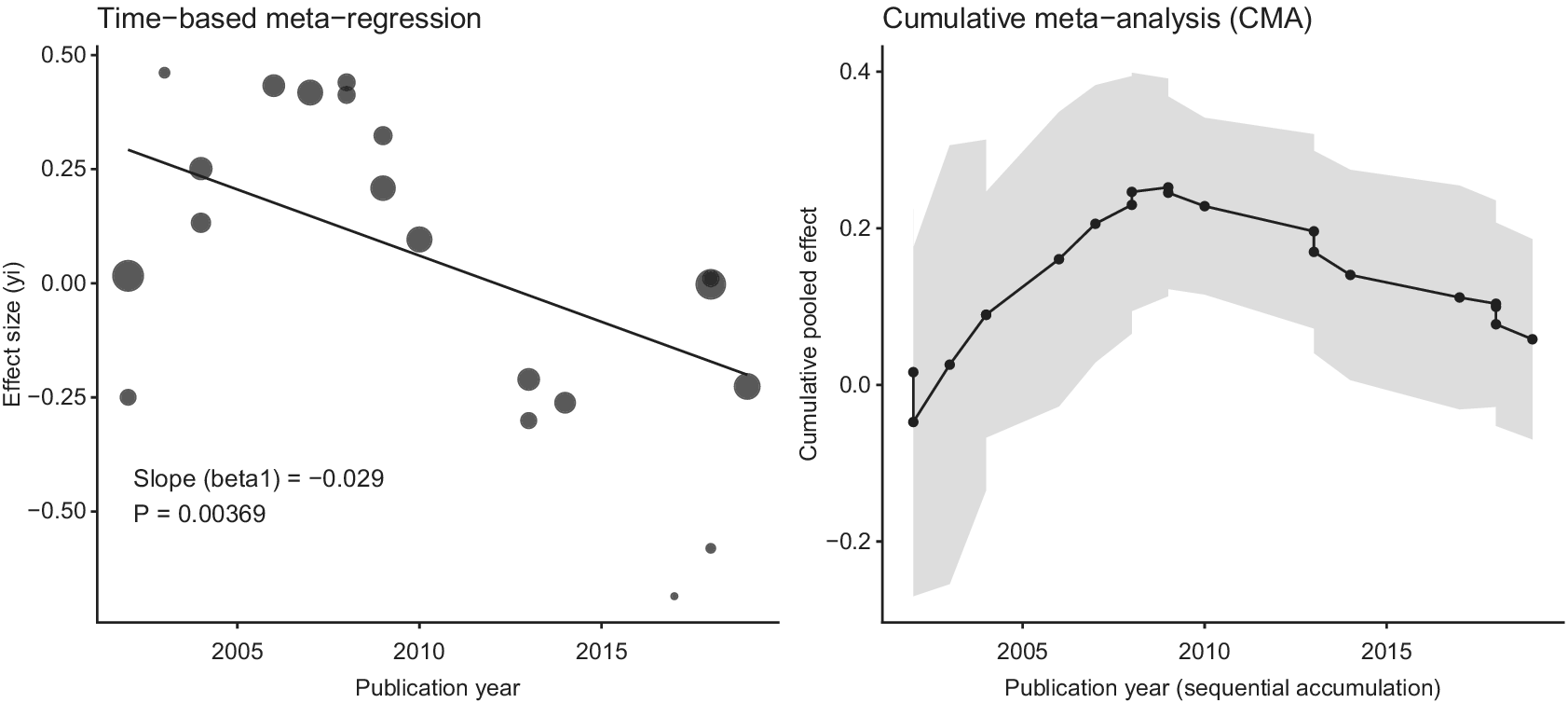Rejecting the null hypothesis, $H_0:\beta _1 = 0$ provides evidence of time-lag bias (Figure 1). A limitation of the commonly used linear meta-regression approach is that it assumes a linear association between effect size and publication time. Although nonlinear meta-regression models could, in principle, be used, meta-analyses often include too few studies to reliably detect or characterize nonlinear temporal patterns.Reference Higgins and Thompson ^{24 ,} Reference Thompson and Higgins ²⁵

Figure 1.

A simulated meta-analysis with time-lag bias presented in chronological order.

Figure 1 Long description

A two-panel visualization of time-lag bias.

Left panel: Time-based meta-regression. The x-axis is publication year from 2005 to 2015. The y-axis is effect size from -0.50 to 0.50. A scatter plot shows circles of varying sizes representing individual studies. A solid black regression line shows a linear decrease from an effect size of approximately 0.3 in 2002 to -0.2 in 2019. Text in the bottom left corner states: slope = -0.029 and P = 0.004.

Right panel: Cumulative meta-analysis (C M A). The x-axis is publication year (sequential accumulation). The y-axis is cumulative pooled effect from -0.2 to 0.4. A line graph with points shows the evolving pooled effect as studies are added chronologically. The line initially rises from near 0 to a peak of approximately 0.25 around 2009, then steadily declines toward 0.05 by 2019. A light gray shaded area surrounding the line represents the confidence interval, which narrows as more studies are accumulated over time.

On the other hand, CMA is a popular method for evaluating and monitoring temporal changes in study results.Reference Kulinskaya and Mah ^{19 ,} Reference Lau, Antman, Jimenez-Silva, Kupelnick, Mosteller and Chalmers ^{26 ,} Reference Antman, Lau, Kupelnick, Mosteller and Chalmers ²⁷ The procedure starts with a single study and sequentially adds additional studies as time progresses. The cumulative effect size shows how the overall estimate changes as an additional study is added. By accumulating studies by publication year, the potential impact of time on effect sizes can be visualized, which helps to suggest whether time-lag bias might exist (Figure 1). If the cumulative effect estimates show a systematic temporal trend, this may suggest time-lag bias, as such patterns can arise when the timing of publication is associated with study results (e.g., larger or statistically significant effects). However, this approach alone cannot confirm the presence of bias and should be supplemented by formal statistical methods. Related approaches, such as trial sequential analysis (TSA), extend this idea by incorporating monitoring boundaries and required information size to assess the stability of accumulating evidence.Reference Xing, Wang and Lin ²³ Although TSA is primarily designed to control type I error in CMA, patterns such as early crossing of significance boundaries followed by attenuation as more studies accumulate may indirectly suggest time-dependent dissemination processes.

Though the aforementioned methods have been widely used in practice,Reference Nakagawa, Lagisz and Jennions ²¹ the simplified parametric assumptions may fail to capture nonlinear or non-monotone dissemination patterns observed in practice, which helps explain the emergence of diverse and heterogeneous forms of time-lag bias beyond the classical paradigms. Complex, nonlinear, or non-monotone dissemination patterns arise because the timing of evidence availability is shaped by multiple, interacting mechanisms rather than a single effect-size-dependent process. Another important mechanism is outcome mismatch between the meta-analysis and the original trials: the outcome synthesized in a meta-analysis may differ from the primary outcome for which the included trials were designed and reported. For example, a meta-analysis may focus on mortality even when mortality was reported only as an adverse event or ancillary outcome in many trials, or on kidney outcomes in trials originally designed around primary cardiovascular outcomes.Reference Kristensen, Rørth and Jhund ^{28 ,} Reference Chan, Hróbjartsson, Haahr, Gøtzsche and Altman ²⁹ In such cases, the timing and completeness of evidence availability for the meta-analytic outcome may differ from those for the original primary outcome, creating more complex temporal patterns. These mechanisms include heterogeneous time-to-publication across study designs, outcomes, and journals; selective outcome reporting that delays the release of certain endpoints; evolving incentives and editorial priorities over time; and changes in the research dissemination ecosystem, such as the emergence of trial registries, preprints, and shifts in database indexing and coverage. The increasing use of preprints further complicates the definition of publication time in time-point-based analyses. A study may have multiple relevant dissemination dates, including initial preprint posting, subsequent preprint updates, formal journal publication, and database indexing. Therefore, relying solely on the formal journal publication date may not fully capture when evidence first became publicly available.

2.2. Time-duration-based bias

An alternative approach defines time as the duration between key stages in the research dissemination process, such as the interval from study completion to publication, from manuscript submission to publication, or from trial registration to publication.Reference Xing, Wang and Lin ^{23 ,} Reference Ross, Tse, Zarin, Xu, Zhou and Krumholz ^{30 ,} Reference Hopewell, Clarke, Stewart and Tierney ³¹ In these settings, time-lag bias is reflected in systematic differences in dissemination durations across studies with different characteristics or results. Several empirical investigations have directly examined the association between dissemination duration and study findings, documenting systematic delays for null or unfavorable results.Reference Tsujimoto, Tsutsumi and Kataoka ^{17 ,} Reference Hopewell, Clarke, Stewart and Tierney ^{31 ,} Reference Reyes, Panza, Martin and Bloch ³² Moreover, when trial completion dates and publication dates are available, time-lag bias can be modeled within a survival analysis framework: “publication” is treated as the event of interest, studies that remain unpublished by the end of follow-up are treated as censored, and Kaplan–Meier estimators or Cox proportional hazards models are used to compare time-to-publication distributions or publication hazards across result types.Reference Tsujimoto, Tsutsumi and Kataoka ^{17 ,} Reference Hopewell, Clarke, Stewart and Tierney ^{31 ,} Reference Reyes, Panza, Martin and Bloch ³² Nevertheless, these survival-based approaches do not fully eliminate modeling challenges. Similar to regression-based methods that use publication time as a covariate, they may be sensitive to nonlinear or nonproportional temporal patterns, particularly when the association between study results and publication hazard changes over follow-up.

However, several methodological challenges should be considered when applying survival analysis to investigate time-lag bias. First, accurate information on trial completion dates, submission dates, or publication dates is not always available or may be inconsistently reported across studies. Misclassification of these time points can lead to biased estimates of time-to-publication distributions. Second, unpublished studies are often unobserved rather than merely censored, which can introduce informative censoring and potentially distort hazard estimates. Third, time-to-publication may be influenced by multiple factors beyond study results, such as trial size, funding source, journal selection, or field-specific editorial practices. Finally, survival models typically assume proportional hazards or other parametric structures that may not represent complex dissemination processes.

Importantly, the presence of a longer-than-usual time interval alone does not constitute time-lag bias. Some degree of delay between study completion and publication is inevitable in the research process due to manuscript preparation, peer review, and editorial procedures. Bias arises when publication delays are systematically associated with the magnitude or direction of study effects, or with study characteristics that are themselves related to effect estimates. For example, if trials with statistically significant or favorable findings have a shorter time interval to be published than trials with null results, early evidence syntheses will disproportionately include positive studies, while null or unfavorable studies remain unpublished or appear later. As a consequence, the evidence available at a given time point may provide a distorted picture of the true intervention effect.

3.1. Classical time-lag bias: Earlier publication of positive findings

In the classical formulation of time-lag bias, studies reporting statistically significant or favorable results tend to be disseminated more rapidly than studies with null or unfavorable findings. As a result, early meta-analyses are often dominated by “positive” evidence, leading to inflated pooled effect estimates and overconfident inference. This phenomenon can arise from multiple, interacting mechanisms. Investigators may be more motivated to submit manuscripts with positive results promptly, journals may prioritize findings perceived as novel or impactful, and null or unfavorable results may undergo longer review processes or be deprioritized. In addition, selective outcome reporting can delay the availability of certain endpoints, particularly when the outcome synthesized in the meta-analysis differs from the primary outcome of the original trial, further skewing the early evidence base and complicating the definition of publication date or time lag for the meta-analytic outcome. In practice, when evidence accrues sequentially and early-appearing studies are disproportionately positive, CMAs may initially overestimate the effect size, followed by attenuation as later, less favorable studies become available. This classical pattern provides a useful baseline for understanding more complex temporal dissemination patterns discussed in Sections 3.2–3.4.

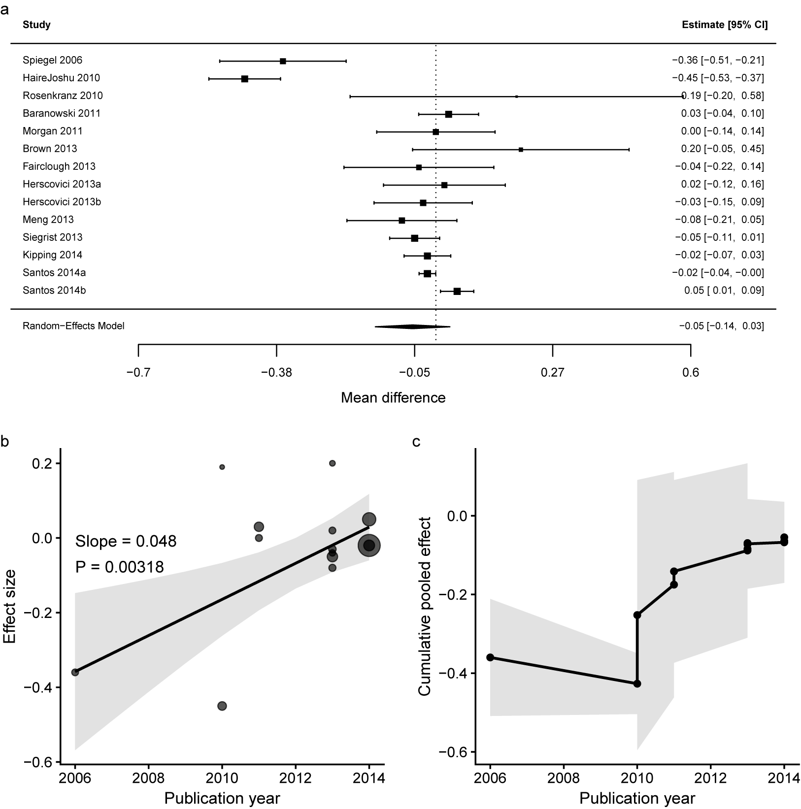
We used a meta-analysis of 14 randomized controlled trials evaluating diet and physical activity interventions versus control among children aged 6–12 years as an example.Reference Brown, Moore and Hooper ³³ The outcome was body mass index z-score (zBMI), and the meta-analytic effect size was defined as the mean difference in zBMI between the intervention and control groups, and Figure 2a displays the corresponding forest plot. When the trials are ordered by publication year, earlier studies tend to report larger and more favorable effects of the intervention relative to control, whereas later studies yield smaller or null effects.

Figure 2.

Plots from a real-world meta-analysis illustrating classical time-lag bias: (a) forest plot; (b) time-based meta-regression bubble plot; and (c) cumulative meta-analysis plot. In panel b, bubble sizes are proportional to the inverse-variance weights of the individual studies, the solid line represents the fitted linear association between effect size and publication time, and the gray shaded area represents the corresponding 95% CIs. In panel c, the black points and connecting line represent the cumulative pooled estimates obtained as studies are added sequentially according to publication time, and the gray shaded area represents the corresponding 95% CIs.

Figure 2 Long description

Panel A is a forest plot listing 14 studies from Spiegel 2006 to Santos 2014b. The x-axis represents mean difference from minus 0.7 to 0.6. A vertical dotted line marks the null effect at minus 0.05. Individual study estimates are shown as squares with horizontal error bars. A diamond at the bottom represents the Random-Effects Model pooled estimate of minus 0.05 with a 95% C I of minus 0.14 to 0.03.

Panel B is a bubble plot of effect size versus publication year from 2006 to 2014. A solid black regression line shows a positive linear increase with a slope of 0.048 and a P value of 0.003. Gray shading indicates the 95% C I. Larger bubbles, representing higher inverse-variance weights, are concentrated in the later years around 2013 and 2014.

Panel C is a cumulative meta-analysis plot. The x-axis is publication year and the y-axis is cumulative pooled effect. A black line with circular points tracks the pooled estimate as studies are added chronologically. The line starts at minus 0.36 in 2006, drops slightly in 2010, and then shows a steady upward trend toward the null, ending near minus 0.05 in 2014. A gray shaded area represents the narrowing 95% C I as more data is included.

This temporal pattern is consistent with the classical formulation of time-lag bias, in which studies with statistically significant or favorable findings are disseminated earlier and therefore disproportionately influence early meta-analytic summaries. As less favorable evidence accumulates over time, the pooled estimate attenuates toward the null, illustrating how meta-analytic conclusions can be inflated early on and subsequently weakened as the evidence base matures (Figures 2b and 2c). Panels b and c provide complementary information about temporal patterns in the accumulated evidence. In panel b, the bubble sizes are proportional to the inverse-variance weights of the individual studies, the solid line represents the fitted linear association between effect size and publication time, and the gray shaded area represents the 95% CIs around the fitted line. The reported P-value tests whether the linear meta-regression slope differs from zero. However, a nonsignificant slope does not exclude nonlinear, non-monotone, or time-localized temporal patterns. In panel c, the black points and connecting line represent the cumulative pooled estimates obtained as studies are added sequentially according to publication time, and the gray shaded area represents the corresponding 95% CIs. The intervals are generally wider during the early stages because fewer studies are available and tend to narrow as evidence accumulates. Cumulative meta-analysis is primarily a descriptive diagnostic: changes in the magnitude, direction, or statistical significance of the cumulative estimate may indicate temporal instability, but no universally accepted objective threshold based on panel c alone establishes the presence of time-lag bias. Such changes may also reflect random variation or genuine clinical or methodological differences among studies. Panel c should therefore be interpreted together with panel b, study characteristics, and contextual information about the dissemination process. In this example, the outcome was zBMI. Because lower zBMI generally indicates a more favorable weight-related outcome in childhood obesity prevention, negative values indicate lower zBMI in the intervention group and therefore favor the intervention, whereas positive values favor the control group. In the context of time-lag bias, this pattern suggests that the later studies yielded smaller or null effects.

3.2. Inverse time-lag bias: Earlier availability of null or unfavorable findings

Inverse time-lag bias arises when null, negative, or unfavorable findings become available earlier than more favorable results, leading to an apparent deflation of early pooled estimates. Although this pattern may seem counterintuitive under the conventional view that favorable or statistically significant findings are disseminated more rapidly, several settings may favor earlier dissemination of null or negative results. As discussed by IoannidisReference Ioannidis ⁹ , inverse publication or reporting bias may occur when null or negative findings are themselves considered informative or desirable, including non-inferiority studies, adverse-event or drug-toxicity studies, and other reassurance-oriented research settings in which evidence of no difference, no harm, or lack of a safety signal may be more publishable or more rapidly reported.Reference Hazell and Shakir ^{34 ,} Reference Zhu, Chen, Chen, Xu, Chen and Liu ³⁵ In post-marketing or regulatory settings, for example, findings suggesting lack of benefit, potential harm, or reassuring safety profiles may be prioritized for rapid dissemination. Similarly, in non-inferiority or equivalence settings, studies showing no clinically meaningful disadvantage may be viewed as favorable, even though they are statistically “null” in the conventional superiority-testing framework.Reference Blanco-Perez and Brodeur ³⁶ In evidence synthesis, this mechanism can produce temporal patterns in which early cumulative pooled estimates lie closer to the null or suggest harm, whereas later studies shift the pooled estimate toward benefit. In time-based meta-regression, this may appear as an increasing treatment benefit over publication time, reversing the direction expected under classical time-lag bias. Therefore, time-lag bias should not be viewed as inherently monotone or necessarily favoring early exaggerated benefit. Depending on the clinical context, study design, outcome type, and dissemination incentives, early meta-analytic conclusions may be biased either toward or away from benefit.

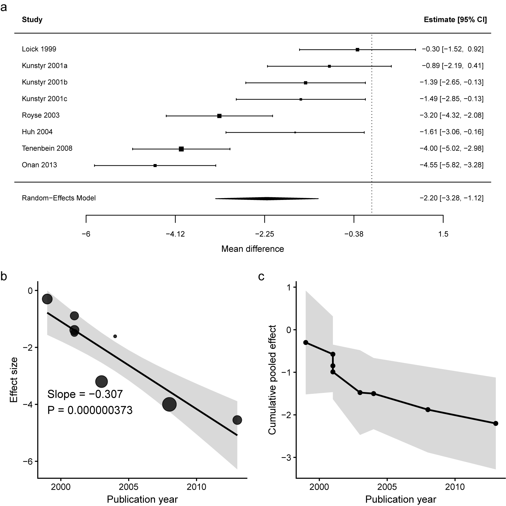
In a meta-analysis of epidural versus systemic analgesia, the outcome pain on movement/coughing at 24 hours was reported as a continuous measure, with data available as mean and standard deviation, enabling synthesis using mean difference.Reference Guay and Kopp ³⁷ Figure 3a illustrates how early estimates can cluster around null or modest effects, with later studies showing increasingly favorable effects, producing a downward temporal drift of the effect size away from 0, and yielding an overall pooled estimate that is substantially more favorable than early impressions. Although these issues may also be relevant to classical time-lag bias, our focus here is on the inverse setting, in which later, more favorable results are slower to emerge. This may occur because beneficial outcomes require longer follow-up, more complex ascertainment, or delayed dissemination (Figure 3b). Regardless of the underlying drivers, the meta-analytic implication is the same: early CMAs may underestimate benefit (Figure 3c), and conclusions based on the early evidence base can be systematically conservative.

Figure 3.

Plots from a real-world meta-analysis illustrating inverse time-lag bias: (a) forest plot; (b) time-based meta-regression bubble plot; and (c) cumulative meta-analysis plot.

Figure 3 Long description

Panel A is a forest plot. The x-axis represents mean difference from minus 6 to 1.5. A vertical dashed line marks the null effect at 0. Eight studies are listed vertically: Loick 1999, Kunstyr 2001a, 2001b, 2001c, Royse 2003, Huh 2004, Tenenbein 2008, and Onan 2013. Each study has a square point estimate and horizontal 95 percent C I bars. The estimates generally shift further left (more negative) over time. A random-effects model diamond at the bottom shows a pooled estimate of minus 2.20 with a 95 percent C I of minus 3.28 to minus 1.12.

Panel B is a bubble plot. The x-axis is publication year from 2000 to 2010. The y-axis is effect size from 0 to minus 6. Gray circles of varying sizes represent individual studies. A solid black regression line shows a steep linear decrease over time. Text indicates slope equals minus 0.307 and P equals le 0.001. A light gray shaded area represents the confidence interval around the regression line.

Panel C is a cumulative meta-analysis plot. The x-axis is publication year from 2000 to 2010. The y-axis is cumulative pooled effect from 1 to minus 3. A black line with circular nodes tracks the pooled effect as each study is added chronologically. The line shows a sharp downward trend, starting near 0 in 1999 and ending near minus 2.2 in 2013. A light gray shaded area represents the narrowing confidence interval as more data is accumulated.

3.3. Non-monotone time-lag bias: Cyclical dissemination patterns

In some research areas, the availability of evidence over time exhibits cyclical or oscillatory patterns rather than monotone trends. Under non-monotone time-lag bias, early meta-analytic estimates may be inflated, attenuated in intermediate stages, and subsequently re-inflated or even reversed as different waves of studies become available. Such patterns can arise from shifting research agendas, funding cycles, and periodic bursts of interest following landmark trials, regulatory actions, or guideline updates.Reference Ioannidis and Trikalinos ^{38 ,} Reference Ioannidis ³⁹ For example, initial enthusiasm surrounding a novel intervention may trigger a wave of small, early-phase studies reporting favorable results, followed by larger confirmatory trials with more modest or null effects, and later by targeted subgroup analyses or implementation studies that again yield heterogeneous or directionally different findings. Additional drivers include changes in editorial priorities, methodological standards, and dissemination channels over time, such as the rise of preprints or registry-based reporting. These dynamics can generate oscillatory trajectories in pooled estimates and apparent “reversals” at different stages of evidence accrual. Under this scenario, CMA may exhibit sign reversals or alternating inflation and attenuation, while linear time-based meta-regression may fail to detect any temporal association despite pronounced non-monotone distortions.

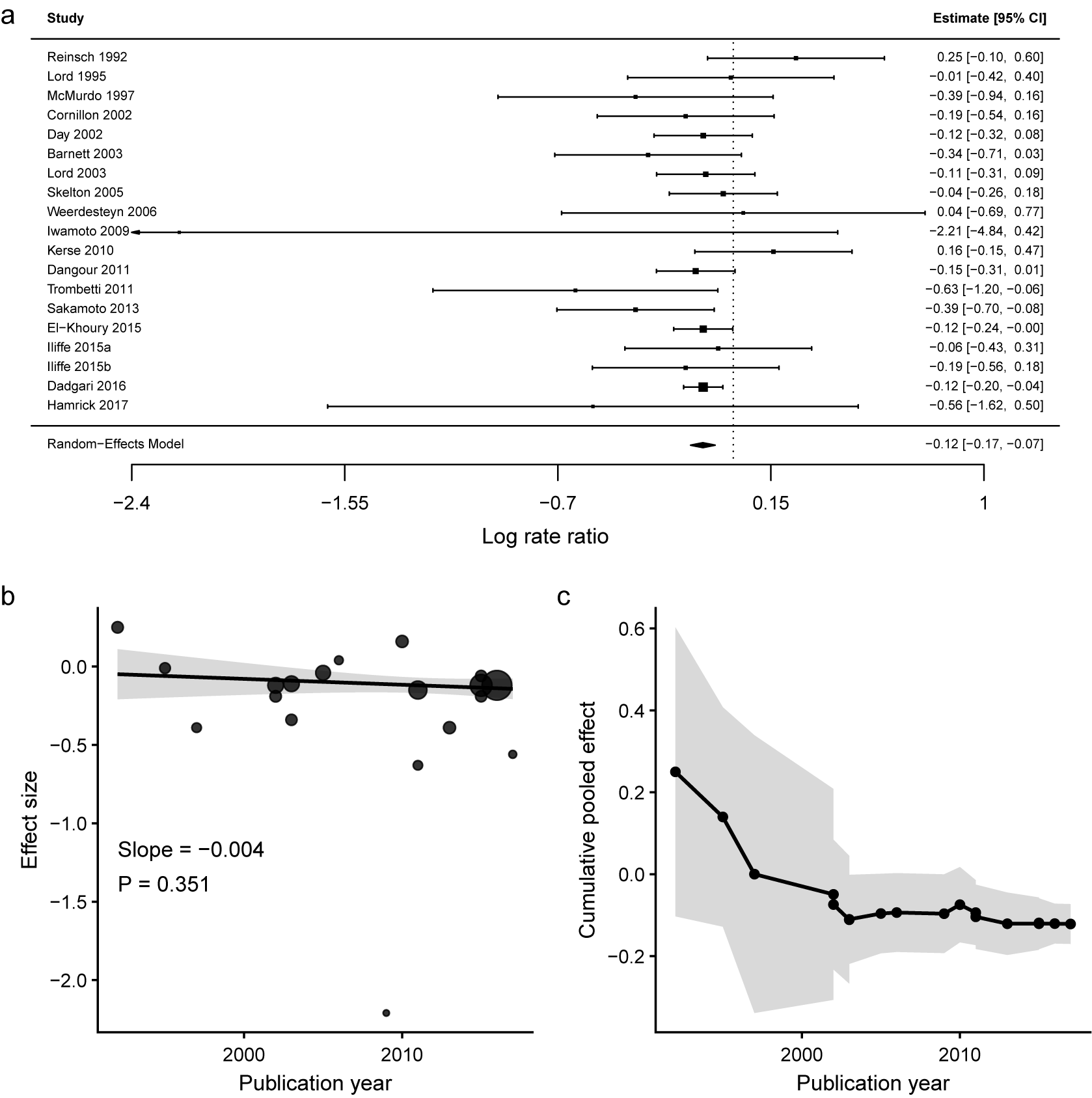
The case study focused on the subgroup of participants not selected for higher risk of falling from Sherrington et al.,Reference Sherrington, Fairhall and Wallbank ⁴⁰ which evaluated whether balance and functional exercise interventions reduce the rate of falls among community-dwelling older adults. A total of 19 trials were included, and the effect size was measured as the log rate ratio, with negative values favoring exercise and positive values favoring control. When trials were ordered by publication year, the pooled trajectory exhibited a non-monotone pattern: early studies suggested modest benefits, mid-period trials attenuated toward the null, and later studies showed renewed evidence of benefit or heterogeneity (Figure 4a). This oscillatory pattern may reflect successive waves of evidence corresponding to shifts in research emphasis, trial design, or intervention implementation.Reference Sterne, Gavaghan and Egger ⁴¹ Despite these temporal distortions in the pooled estimates, conventional time-based meta-regression did not detect a clear association between effect size and publication time (slope $= -0.004$ , $P = 0.351$ ) (Figures 4b and 4c). This case illustrates the limitations of diagnostics that assume simple monotone temporal trends and motivates methods that remain informative under more general, non-monotone dissemination processes.

Figure 4.

Plots from a real-world meta-analysis illustrating non-monotone time-lag bias: (a) forest plot; (b) time-based meta-regression bubble plot; and (c) cumulative meta-analysis plot.

Figure 4 Long description

Panel A is a forest plot listing 19 studies from Reinsch 1992 to Hamrick 2017. The x-axis represents the log rate ratio from -2.4 to 1. Each study is shown with a point estimate and horizontal 95 percent C I bars. A vertical dashed line marks the null effect at 0. At the bottom, a diamond represents the random-effects model with a pooled estimate of -0.12 [-0.17, -0.07].

Panel B is a bubble plot showing effect size on the y-axis against publication year on the x-axis from 1990 to 2020. Circles of varying sizes represent individual studies. A regression line shows a slight downward trend with a slope of -0.004 and a P value of 0.351. A shaded gray area represents the confidence interval around the regression line.

Panel C is a cumulative meta-analysis plot. The y-axis is the cumulative pooled effect and the x-axis is the publication year. A black line with circular markers tracks the evolving pooled estimate as studies are added chronologically. The line starts at a positive effect near 0.25 in the early 1990s and trends downward, stabilizing below 0 after the year 2000. A wide gray shaded area indicates the narrowing 95 percent C I as more data is accumulated.

Importantly, this oscillatory trajectory should not be interpreted as definitive evidence that time-lag bias occurred in this meta-analysis. The observed pattern is potentially consistent with time-dependent selective dissemination, but it may also reflect random variation, differences in study populations or methodological quality, changes in intervention implementation, or successive waves of research conducted in different clinical settings. Confirmation of time-lag bias would require additional evidence that the timing of study availability was systematically associated with study findings or related characteristics. Nevertheless, the pattern illustrates a potential limitation of conventional analyses: opposing changes across different periods may produce a linear meta-regression slope close to zero even when the cumulative pooled estimate changes meaningfully in magnitude, direction, or statistical significance over time.

3.4. “Anomalous evidence” concentrated in a specific time window

In practice, apparent time trends in meta-analytic effect estimates do not always reflect a genuine time-lag dissemination process. A common alternative is a localized shock: one or a few outlying or otherwise anomalous studies appearing in a particular period, producing a sharp jump or dip in the time-ordered series. The signature of this scenario is a non-smooth evolution; rather than a gradual monotone drift, the trajectory exhibits an abrupt change within a specific time window, and the pooled estimate may remain distorted thereafter or return toward earlier levels once additional studies accrue.

Such time-localized outliers can arise through several real-world mechanisms.Reference Baujat, Mahé, Pignon and Hill ^{42 ,} Reference Viechtbauer and Cheung ⁴³ Changes in clinical practice or study design during a particular era (e.g., adoption of new surgical techniques, perioperative management protocols, anticoagulation strategies, monitoring practices, or revised outcome definitions) may complicate comparisons with earlier or later studies. Measurement and reporting conventions can also shift over time, including changes in scales, follow-up windows, analysis definitions, or endpoint adjudication procedures, creating an artificial “period effect.” Alternatively, the affected period may contain studies with a high risk of bias or data anomalies, generating extreme estimates without any systematic dissemination ordering. Localized outliers can be misleading because they may trigger sudden changes in direction or statistical significance in CMA; a few high-leverage studies can drive time-based meta-regression slopes, creating spurious evidence of time-lag bias.

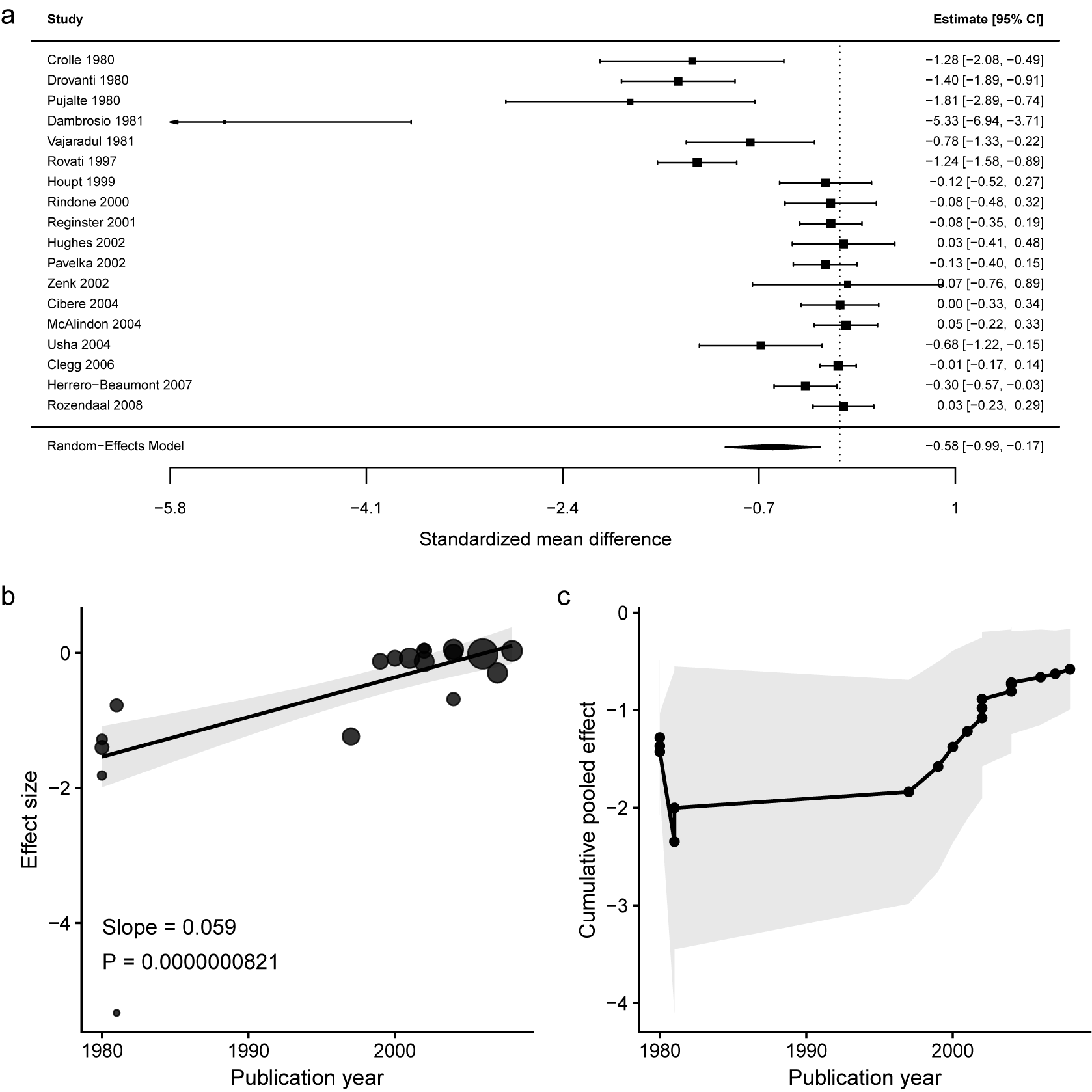
To illustrate a time-localized anomalous pattern in evidence accumulation, we reanalyzed the pain outcome from a Cochrane review comparing glucosamine versus placebo for osteoarthritis.Reference Towheed, Maxwell and Anastassiades ⁴⁴ The outcome was pain severity, and the effect size was defined as the standardized mean difference in pain scores between the glucosamine and placebo groups. Because lower pain scores indicate greater symptom improvement, negative effect estimates favor glucosamine, whereas positive estimates favor placebo. The apparent temporal pattern is dominated by a localized cluster of extreme effects in the early window around 1980–1981 rather than by a smooth dissemination-driven drift. Several early trials show large negative effect sizes favoring glucosamine, including one highly extreme estimate, while the later evidence base from the late 1990s through 2008 contains many trials with estimates close to the null and CIs frequently overlapping 0 (Figure 5a). This visual step change is consistent with time-localized anomalous or outlier influence. In CMA, these early studies induce abrupt level shifts, while in meta-regression, they can drive the estimated temporal slope away from zero, creating apparent evidence of time-lag bias even in the absence of a genuine dissemination-driven temporal process (Figures 5b and 5c).

Figure 5.

Plots from a real-world meta-analysis illustrating time-lag bias with anomalies concentrated within a specific time window: (a) forest plot; (b) time-based meta-regression bubble plot; and (c) cumulative meta-analysis plot.

Figure 5 Long description

The figure consists of three panels labeled A, B, and C.

Panel A is a forest plot. The left column lists 18 studies from Crolle 1980 to Rozendaal 2008. The center contains a horizontal axis for standardized mean difference ranging from minus 5.8 to 1. A vertical dashed line represents the null effect at 0. Individual study effects are shown as black squares with horizontal error bars representing 95 percent C I. Earlier studies (1980 to 1981) show large negative effects, while later studies (2000 to 2008) cluster around the null line. At the bottom, a diamond represents the random-effects model estimate of minus 0.58 [-0.99, -0.17].

Panel B is a meta-regression bubble plot. The x-axis is publication year from 1980 to 2010, and the y-axis is effect size from minus 4 to 0. A positive linear regression line shows a slope of 0.059 with a P value le 0.001. Bubbles representing studies increase in size and move upward toward zero as time progresses, indicating that more recent studies report smaller effect sizes.

Panel C is a cumulative meta-analysis plot. The x-axis is publication year from 1980 to 2010, and the y-axis is cumulative pooled effect from minus 4 to 0. A black line with circular nodes tracks the pooled effect over time, surrounded by a light gray shaded area for the confidence interval. The line shows a sharp initial drop followed by a steady upward trend toward zero starting around the year 2000.