1. Introduction
In recent years, with the rapid development of computer technology, sensor technology, and artificial intelligence, multi-robot collaborative technology has been widely used in search and rescue [Reference Wang, Wang, Ding, Liu, Wang, Fan, Bai, Hongbiao and Du1–Reference Du3], inspection [Reference Song, Cheng, Qi and Zou4, Reference Best and Hollinger5], and pollution source localization [Reference Zhang, Qin, Tang and Li6, Reference Wiedemann, Vlaicu, Josifovski and Viseras7]. Multi-robot systems effectively complete complex tasks through self-organized cooperative control, which is often beyond the capability of a single robot [Reference Gundana and Kress-Gazit8–Reference Queralta, Li, Schiano and Westerlund10]. Compared to individual robots, multi-robot collaborative formation has the following advantages [Reference Zhou, Wang, Wang and Dong11–Reference Orr and Dutta13]:
-
(1) Multiple robots can collaboratively complete given tasks, significantly enhancing work efficiency.
-
(2) Due to the weaker ability of individual robots in handling multiple tasks, collaborative work can compensate for individual shortcomings, expanding the application scenarios and capabilities.
-
(3) Multi-robot systems can execute different tasks simultaneously, greatly improving task completion efficiency.
-
(4) Robots in a cluster system complement each other and have fault tolerance. Even if an individual robot fails to perform a task due to malfunctions, other robots can substitute and complete the task, enhancing system fault tolerance, robustness, and flexibility.
-
(5) Leveraging resource distribution characteristics within the system reduces the cost of individual robots and simplifies system design, reducing losses when executing hazardous tasks.
Based on these advantages, multi-robots can efficiently and accurately complete tasks such as area coverage and source localization in complex environments. However, the prerequisite for completing these tasks is to develop a reasonable coverage strategy, enabling robots to make autonomous decisions and select positions with maximum benefits.
In the field of coverage and source localization in unknown environments, there has been extensive research [Reference Renzaglia and Briñón-Arranz14–Reference Chen, Yang, Huang, Leng and Fu16]. Literature reviews indicate that research on source localization using multi-robots often employs techniques such as density gradients [Reference Karagüzel, Turgut, Eiben and Ferrante17–Reference Chang, Shan, Zhang and Dai19], information entropy [Reference Jang, Park and Oh20–Reference An, Park and Oh22], or Bayesian methods [Reference Ma, Zhang, Wu, Calmon and Li23–Reference Newaz, Alsayegh, Alam and Bobadilla25]. Density gradient methods utilize local gradient information for target localization, adapting to real-time environmental changes and not relying on prior map information. A method combining gradient and probabilistic search for source localization is proposed in ref. [Reference Yungaicela-Naula, Zhang, Garza-Castañon and Minchala26]. The gradient method is used for UAV navigation and tracking, while probabilistic search is used to estimate the position of contaminants, reducing search time and area through the combination of these two methods. However, gradient methods are prone to local optima, especially in complex environments, which may affect the accuracy and efficiency of source localization. Some scholars use deep reinforcement learning methods to guide robot motion. Without relying on prior map information, robots interact with the environment, learning optimal pollution source localization strategies through exploration and environmental feedback. A method based on deep reinforcement learning for indoor odor source localization is proposed in ref. [Reference Li, Yuan and Yuan27], modeling the odor source localization problem as a Markov decision process and designing state space, action space, and dense rewards to address sparse reward issues, finally generating the robot’s optimal decision through the proximal policy optimization algorithm. Ref. [Reference Hu, Niu, Carrasco, Lennox and Arvin28] considers the problem of multi-robot cooperative exploration in unknown environments, combining Voronoi diagrams with deep reinforcement learning strategies to dynamically divide Voronoi regions based on robot movement in the environment and complete obstacle avoidance based on deep reinforcement learning methods. While this method yields good search results, it still faces potential challenges and limitations such as sample complexity and long training times. Intelligent optimization algorithms simulate collective behaviors of birds or fish, enabling all individuals to reach a global optimum through mutual cooperation. Ref. [Reference Feng, Cai, Yang, Xu, Jiang, Li, Li and Yan29] proposes a multi-robot olfaction method independent of airflow information. This method utilizes particle swarm search to track odor sources and broadens the robot’s search range by introducing extreme perturbation beacons to prevent robots from getting stuck in local extremes. However, the drawbacks of heuristic intelligent algorithms lie in slow convergence speed, difficulty in modeling environmental fields, and poor interpretability of the algorithm. To address this issue, ref. [Reference Luo, Nam, Kantor and Sycara30] adopts the Gaussian Mixture Model method to predict the environmental model, guiding robots to explore and reconstruct the environment based on the Voronoi diagram method. The advantage of this method is its ability to reconstruct unknown environmental models, but it exhibits high computational complexity when dealing with large-scale datasets, requiring significant storage and computing resources, leading to longer training times.
In terms of multi-robot collision avoidance, common methods include artificial potential field methods [Reference Zhen, Chen, Wen and Han31–Reference Gao, Bai, Fu and Quan33], A* [Reference Zhong, Tian, Hu and Peng34–Reference Kiadi, García, Villar and Tan36], and reinforcement learning methods [Reference Wang, He, Cao, Ma, Li, Jia and Cui37–Reference Tan39]. However, the artificial potential field method is prone to trapping robots in local optima, and unreasonable potential field functions may prevent robots from finding the global optimal path. The performance of the A* method highly depends on the choice of heuristic function, and in cases of large or complex search spaces, the time complexity of the A* algorithm may be high, leading to slow search speeds, making it unsuitable for applications with high real-time requirements. Reinforcement learning methods require a large amount of trial and error to train the model, resulting in low sample efficiency, requiring significant time and resources to obtain sufficient empirical data. The drawbacks of existing obstacle avoidance methods mainly lie in local optima and low convergence speed, both of which may prevent robots from completing the assigned tasks. Compared to traditional path planning methods, multi-robot control methods based on Voronoi diagrams allow each robot to generate its own Voronoi region based on its position and the surrounding environment, enabling distributed path planning and control [Reference Zhu, Cheng, Zhang, Zhang and Liu40, Reference Chen, Guo and Li41]. Additionally, the boundaries of Voronoi regions can be used to avoid collisions between robots, as each robot will only move within its allocated region. This collision avoidance mechanism can enhance system safety and efficiency. In the author’s research, ref. [Reference Cao, Chen, Gao, Dang and An42] considers communication constraints and large localization errors during the formation process. It enhances collision avoidance capabilities by constructing buffer Voronoi cells for each robot and imposes communication distance constraints on Voronoi regions to simulate communication-limited environments. Finally, obstacle avoidance strategies are designed to achieve formation control in non-convex environments. Ref. [Reference Wang, Xi, Ding and Chen43] proposes a multi-robot encirclement method based on buffered Voronoi cells. This method utilizes separate hyperplanes and buffers to create Voronoi regions that ensure robot safety, devising pursuit control laws to enable robots to swiftly encircle evaders. The buffered Voronoi method can avoid robot collisions while maintaining fast computational speeds, overcoming the shortcomings of traditional path planning methods. Furthermore, this method does not require kinematic and dynamic modeling of robots, making it easier to deploy on actual robots.
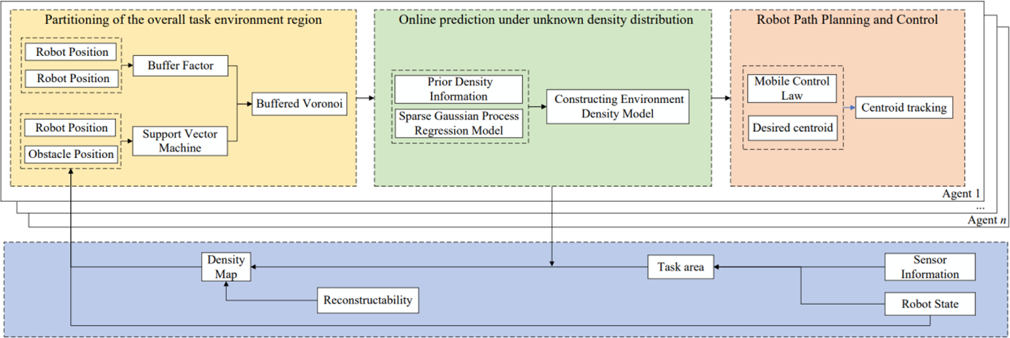
Therefore, this paper proposes a new framework that uses a multi-robot control strategy based on Centroidal Voronoi Tessellation (CVT) to address the problems of area coverage and source localization in unknown environments. This framework first ensures the safety of the multi-robot formation, then reconstructs the distribution of the unknown field, and determines the exact location of the pollution source. It is worth noting that the entire process operates online, meaning that robots autonomously make decisions to accomplish the assigned tasks. The overall framework is illustrated in Figure 1.
Overview of the overall framework.

This paper makes three main contributions: Firstly, it addresses the uncertainty of robot positions by enhancing safety between robots through constructing buffered Voronoi cells. Secondly, it proposes an online multi-robot coverage algorithm based on CVT, which constructs a density function model of the unknown environment using the Variational Sparse Gaussian Process Regression (VS-GPR) method, and plans task areas and exploration target points for robots by introducing the centroid Voronoi partition algorithm with uncertainty. Lastly, it designs formation control laws and proves the stability of the algorithm through Lyapunov stability analysis, thereby achieving formation coverage and source localization in unknown areas.
The structure of the remaining parts of the paper is as follows: Section 2 introduces the basic theory of multi-robot safety control. Section 3 proposes an online coverage and source localization algorithm based on VS-GPR and proves the stability of the system by constructing a Lyapunov function. Section 4 provides corresponding simulation results and analysis. Section 5 validates the effectiveness of the algorithm through UAV experiments. The conclusion and future prospects are presented in Section 6.
2. Multi-robot area coverage safety control
2.1. Coverage function
After obtaining the location information of n robots, it is necessary to design a region coverage method to drive each robot towards its target point in order to achieve optimal coverage of the task area. The Voronoi diagram assigns non-overlapping regions to each robot, and can dynamically update the shape and size of the Voronoi regions following the iterative dynamics of the robots.
In the environment
 ${\Omega} \subseteq \mathrm{{R}}^{N}$
, let
 $E=\{e_{1},e_{1},\ldots, e_{n}\}$
be the set of n robots,
 $P=\{p_{1},p_{1},\ldots, p_{n}\}$
be the set of robot positions, and the definition of Voronoi cells is as follows:
 \begin{equation} V_{i}=\{p\in {\varOmega }\mid \| q-p_{i}\| \lt \| q-p_{j}\|, \forall j\neq i\} \end{equation}
where
 $i,j=1,\ldots, n, \| \cdot \|$
represents the Euclidean norm on
 $\mathrm{{R}}^{N}$
.
Given the density function
 $\rho$
, the objective function for region coverage is
 \begin{equation} \mathrm{{H}}\!\left(p_{1},\ldots, p_{n}\right)=\sum _{i=1}^{n}\int _{{V_{i}}}\left\| q-p_{i}\right\| ^{2}\rho \!\left(q\right)\textit{d}q \end{equation}
According to the inertia theory, the mass
 $M_{{V_{i}}}$
and the centroid
 $C_{{V_{i}}}$
of Voronoi cells can be expressed as:
 \begin{equation} M_{{V_{i}}}=\int _{{V_{i}}} \rho \!\left(q\right)dq \end{equation}
 \begin{equation} C_{{V_{i}}}=\frac{1}{M_{{V_{i}}}}\int _{{V_{i}}} q\rho \!\left(q\right)dq \end{equation}
In addition,
 $J_{{V_{{p_{i}}}}}$
represents the polar moment of inertia of the
 $i$
-th robot.
 \begin{equation} J_{{V_{{p_{i}}}}}=\int _{{V_{i}}} \left\| q-p_{i}\right\|^{2}\rho \!\left(q\right)dq \end{equation}
According to the parallel axis theorem, this can be further expressed as follows:
 \begin{equation} J_{{V_{{p_{i}}}}}=J_{{V_{{c_{i}}}}}+M_{{V_{i}}}\left\| p_{i}-C_{{V_{i}}}\right\| ^{2} \end{equation}
where
 $J_{{V_{{c_{i}}}}}$
represents the polar moment of inertia of the Voronoi region around its centroid.
Another form of
 $H(P)$
can be derived from Eq. (6):
 \begin{equation} H\!\left(P\right)=\sum _{i=1}^{k} J_{{V_{{c_{i}}}}}+\sum _{i=1}^{k} M_{{V_{i}}}\left\| p_{i}-C_{{V_{i}}}\right\| ^{2} \end{equation}
Then, the derivative of
 $H(P)$
with respect to its pair in Eq. (7) is
 \begin{equation} \frac{\partial H\!\left(P\right)}{\partial p_{i}}=2M_{{V_{i}}}\!\left(p_{i}-C_{{V_{i}}}\right) \end{equation}
The expression for the control law is
 \begin{equation} u_{i}=2K_{i}M_{{V_{i}}}\!\left(p_{i}-C_{{V_{i}}}\right) \end{equation}
where
 $K_{i}$
is a positive definite gain matrix, usually an identity matrix.
When the robot is at its centroid, the system has the lowest cost function,
 \begin{equation} C_{{V_{i}}}=\textit{arg min }\mathrm{{H}}\!\left(p_{1},\ldots, p_{n}\right)=\frac{\int _{V}q\rho \!\left(\textit{q}\right)dq}{\int _{V}\rho \!\left(q\right)dq} \end{equation}
2.2. Safety buffer Voronoi cell
In robotic systems, the actual position of the robot may be affected by sensor error, communication delay, or environmental interference. Ref. [Reference Urban, ŠTRONER and Kuric44] pointed out that systematic displacement and rotation errors would occur when using the navigation GNSS data on the UAV for geo-reference, resulting in deviations in the collected data. Ref. [Reference Hu, Zhang, Sfarra, Pivarčiová, Yao, Duan, Ibarra-Castanedo, Tian and Maldague45] proposed that unbalanced terahertz line scanning exposure sources would lead to uneven energy distribution, which would affect the accuracy of imaging results. These errors can lead to inaccurate robot path planning, resulting in collisions between robots.
In density-based CVT algorithms, when initializing, agents are generally treated as point masses, ignoring their actual size. In addition, there exist position errors in the agent positioning system, leading to a certain level of uncertainty in the agent’s position information. Traditional CVT algorithms do not consider the two above-mentioned issues, resulting in agents colliding with each other during the process of tracking centroids.
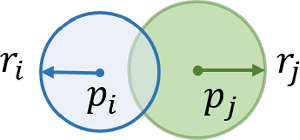
As shown in Figure 2, the blue circle and the blue dot represent the perceptual range and position of robot
 $i$
respectively, while the green circle and the green dot represent the perceptual range and position of robot
 $j$
respectively. Due to sensor error, communication delay, environmental interference, and other factors, the actual position of the robot may cause errors. The position of two robots may be any point within their respective circles, and when the distance between two robots is less than
 $r_{i}$
or
 $r_{j}$
, there is a risk of collision between two robots. The blue and green circles represent the position error upper bounds of agents
 $p_{i}$
and
 $p_{j}$
. In the overlapping area of the position error circles, the agents will collide with each other.
Position error range.

2.2.1. Collision avoidance between robots
To address the issue of collision avoidance between robots, the CVT algorithm is extended by introducing a buffer factor to enhance the obstacle avoidance performance between agents.
Considering a group of n agents moving in the spatial environment
 ${\Omega} \subseteq \mathrm{{R}}^{N}$
, for a set of n agents in
 $\mathrm{{R}}^{N}$
, the Voronoi cell definition of Eq. (1) can be re-expressed as:
 \begin{equation} \mathrm{{V}}_{i}=\left\{p\in \mathrm{{R}}^{N}\mid \left(p-\frac{p_{i}+p_{j}}{2}\right)^{T}\left\| p_{ij}\right\| \leq 0,\forall j\neq i\right\} \end{equation}
where
 $p_{ij}=p_{j}-p_{i}$
. When considering both the actual size of agents and position errors, introducing a buffer region constrains the Voronoi cells. The calculation equation for the buffered centroid Voronoi cell is defined as follows:
 \begin{equation} \mathrm{{V}}_{b,i}=\left\{p\in \mathrm{{R}}^{N}\mid \left(p-\frac{p_{i}+p_{j}}{2}\right)^{T}p_{ij}+\eta _{\textit{ij}}\left\| p_{ij}\right\| \leq 0,\forall j\neq i\right\} \end{equation}
where
 $\eta _{\textit{ij}}$
represents the buffer factor between two agents, and the size of the buffer factor is determined by the position error radius of each agent, that is,
 \begin{equation} \eta _{\textit{ij}}=r_{i}+r_{j} \end{equation}
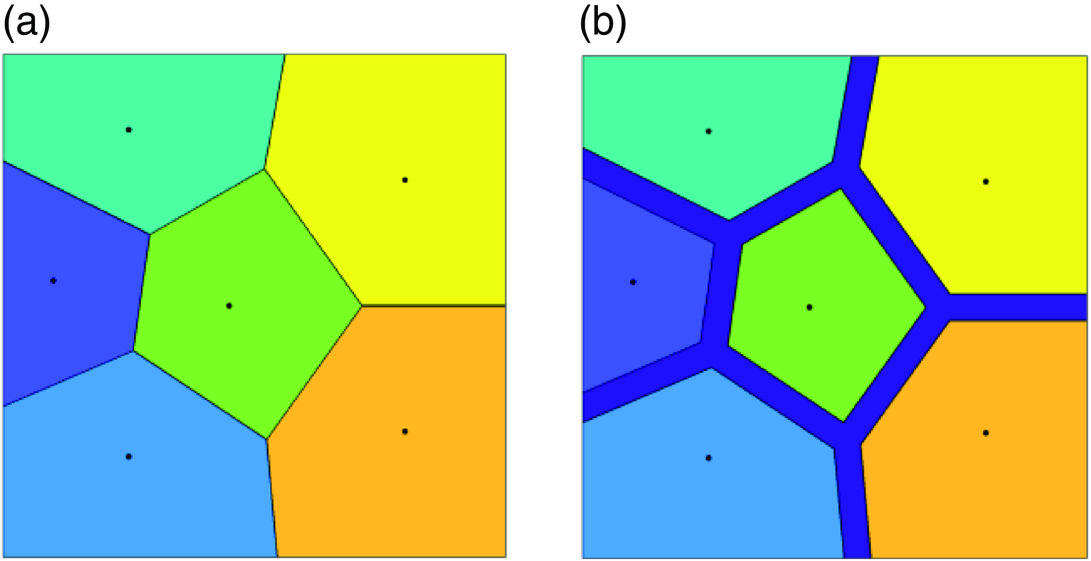
Figure 3 shows two different Voronoi partitions, where Figure 3(a) represents the standard Voronoi partition, while the improved CVT algorithm shrinks the boundaries of Voronoi cells based on the size of agents to ensure their safety, as shown in Figure 3(b).
Two different Voronoi partitions. (a) Standard Voronoi partition. (b) Buffered Voronoi partition.

2.2.2. Mutual avoidance between robots and obstacles
We adopt the support vector machine (SVM) method to partition the safe area between robots and obstacles. The hyperplane between two robots
 $p_{i}$
and
 $p_{j}$
can be represented as:
 \begin{equation} {a_{ij}}^{T}p=b_{ij} \end{equation}
where
 $a_{ij}$
is the normal vector determining the direction of the hyperplane, and
 $b_{ij}$
is the distance term determining the distance between the hyperplane and the origin.
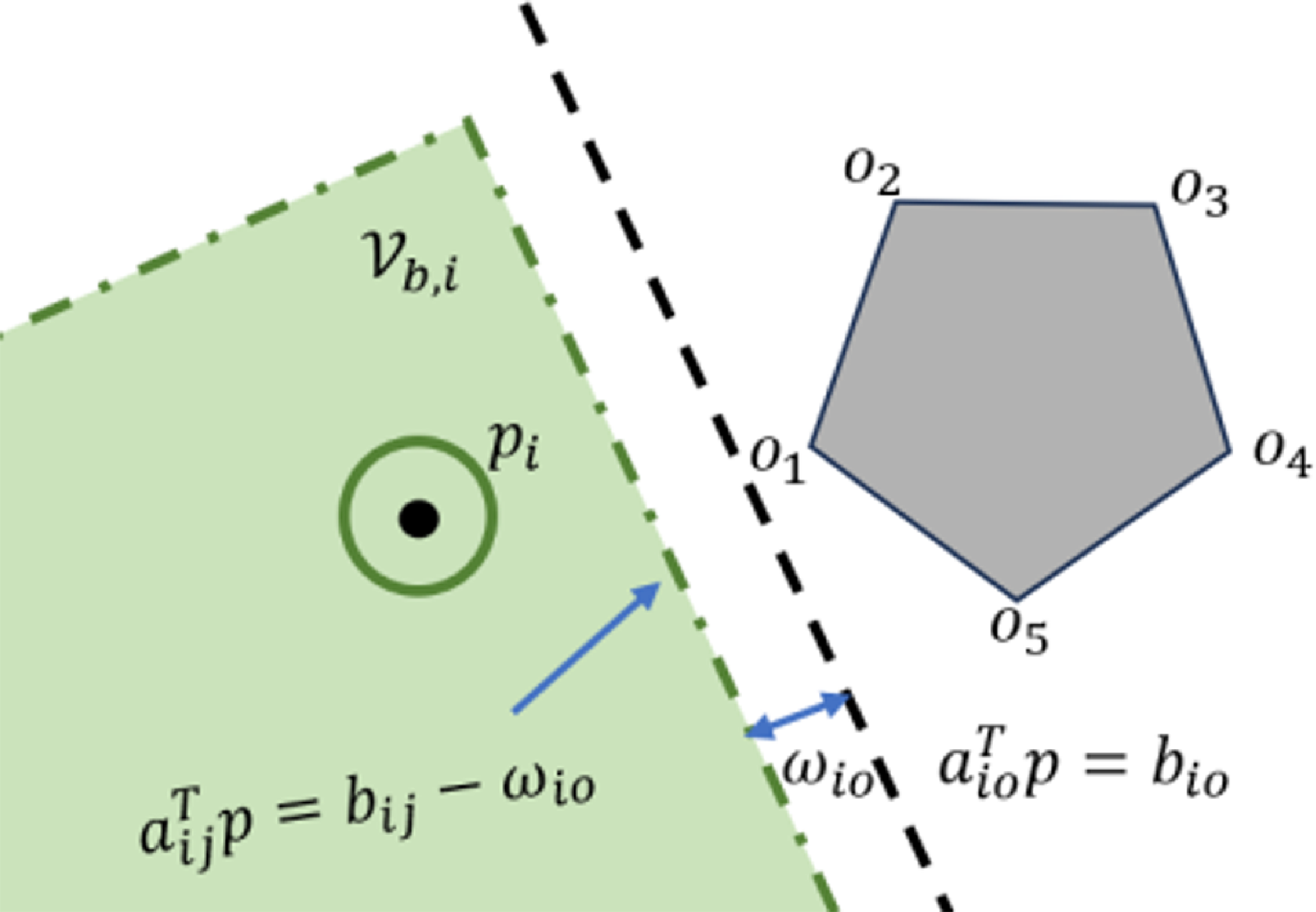
Obstacles generally have irregular characteristics, setting the vertex set of obstacles as
 ${\mathrm{O}}_{m}=\{o_{1},o_{2},\ldots, o_{m}\}$
, and generating safe Voronoi cells by computing the optimal separating hyperplane between robot
 $p_{i}$
and the vertex set of obstacles
 ${\mathrm{O}}_{m}$
, as shown in Figure 4.
Avoidance Voronoi cell.

By solving the following objective optimization problem, the optimal separating hyperplane can be quickly computed.
 \begin{equation} \mathop{\textit{min}}_{a_{io},b_{io}} \frac{1}{2}\mathrm{P} a_{io}\mathrm{P}^{2} \end{equation}
 \begin{equation} \textit{s}\textit{.}\textit{t}\textit{.}\quad y_{i}\!\left({a_{io}}^{T}p_{i}+b_{io}\right)\geq 1 \end{equation}
where
 $y_{i}$
represents the decision function of the support vector machine.
 $a_{io}$
represents the coefficient of the normal vector of the hyperplane, which determines the direction of the hyperplane,
 $\textit{b}_{io}$
represents the bias term of the hyperplane, which determines the position of the hyperplane.
The constraint Voronoi cell between the robot and the obstacle can be represented as
 \begin{equation} \mathrm{{V}}_{i}^{b}=\{p\in {\mathbb{R}}^{d}\;:\;{a_{io}}^{T}p\lt b_{ij}-\omega _{i\textit{o}},i\in n\} \end{equation}
where
 $\omega _{i\textit{o}}=r_{io}a_{io}, \omega _{i\textit{o}}$
represents the buffer term between the robot and the obstacle.
3. Online learning coverage control method based on VS-GPR
3.1. Traditional Gaussian process regression (GPR)
GPR is generally used to reconstruct the distribution of unknown environmental fields. The main process is as follows:
-
(1) Mount sensors on the robot and acquire environmental data through the robot’s movement in the environment.
-
(2) Use the robot’s position and sensor data as inputs, and the distribution of the unknown environment as outputs to train the GPR model.
-
(3) Plan paths for the robot based on the environmental field distribution constructed in the previous step.
Assuming GPR follows a prior Gaussian process with a mean of 0.
 \begin{equation} f\sim GP\!\left(0,k\!\left(x,x'\right)\right) \end{equation}
where
 $k(x,x')$
represents the kernel function of the GPR model. In this paper, the radial basis function is used as the kernel function of GPR.
 \begin{equation} k\!\left(x,x'\right)=M\textit{exp}\!\left(\frac{-\left\| x_{i}-x'_{i}\right\| ^{2}}{2l^{2}}\right) \end{equation}
In the equation,
 $M$
and
 $l$
are hyperparameters, where
 $M$
represents the amplitude scale and
 $l^{2}$
represents the length scale. Reasonably selecting optimal hyperparameters can improve the model’s fitting accuracy. Generally, the maximum likelihood estimation method is used to construct the likelihood function, and its partial derivative is taken to obtain the hyperparameters of GPR.
Considering the regression task
 $y=f(x)+\varepsilon$
, where
 $\varepsilon$
is independently and identically distributed Gaussian noise that follows a distribution
 $\varepsilon \sim N(0,\sigma _{n}^{2})$
. By maximizing the likelihood function, the hyperparameters are obtained.
After knowing the training set inputs, hyperparameters, and information about the test points, the mean and variance of the predictive model are as follows:
 \begin{equation} \mu _{\ast}\!\left(x_{\ast}\right)=K\!\left(x_{\ast},x\right)\left[K\!\left(x,x\right)+\sigma _{n}^{2}I\right]^{-1}y \end{equation}
 \begin{equation} \sigma _{\ast}^{2}\!\left(x_{\ast}\right)=k\!\left(x_{\ast},x_{\ast}\right)-K\!\left(x_{\ast},x\right)\left[K\!\left(x,x\right)+\sigma _{n}^{2}I_{n}\right]^{-1}K\!\left(x,x_{\ast}\right) \end{equation}
GPR is a powerful non-parametric modeling method that can model any shape space and make precise probability predictions. However, computing the covariance matrix of GPR has a time complexity of
 $O(N^{3})$
, making model inference and prediction very difficult with large training set data. Approximate inference methods are needed to reduce complexity in such cases.
3.2. Variational sparse Gaussian process regression
In recent years, the method of sparse Gaussian process regression (SGPR) has developed rapidly, with the core idea of using sparse inducing points to approximate the complete Gaussian process model. Considering the characteristics of online coverage problems, which require fast computation speed and high prediction accuracy, this paper will train the model based on the VS-GPR method, and use it to guide the robot’s motion.
The core of the Variational Free Energy (VFE) method is to approximate the posterior distribution in a variational inference manner. Firstly, the posterior distribution is parameterized by a set of inducing points, and optimization is performed with the goal of minimizing the Kullback-Leibler divergence between the variational distribution and the true posterior distribution. In this process, by adjusting the positions of the inducing points, the variational distribution is gradually made to approximate the true posterior distribution, thereby reducing computational complexity. The following is a specific theoretical introduction to VS-GPR.
Let the set of inducing points be
 $Z=\{z_{i}\}_{i=1}^{M}$
, corresponding to function values
 $\boldsymbol{u}=\{u_{i}\}_{i=1}^{N}=\{f(z_{i})\}_{i=1}^{N}$
. Assuming that given these inducing points, the prediction points are conditionally independent of the training samples,
 \begin{equation} p\!\left(f_{\ast}\mid \boldsymbol{y}\right)=\int p\!\left(f_{\ast}\mid \boldsymbol{u}\right)p\!\left(\boldsymbol{u}\mid \boldsymbol{y}\right)\textit{d}\boldsymbol{u} \end{equation}
The VFE method largely solves the problem of overfitting in prior approximation, and the approximate posterior distribution tends to be closer to the true posterior distribution.
Through Jensen’s inequality, the lower bound of the marginal likelihood can be calculated.

where
 $q(\boldsymbol{f},\boldsymbol{u})$
is called the variational distribution. When
 $q(\boldsymbol{f},\boldsymbol{u})=p(\boldsymbol{f},\boldsymbol{u}\mid \boldsymbol{y})$
is optimal, the equality holds.
The form of
 $q(\boldsymbol{f},\boldsymbol{u})$
is set as:
 \begin{equation} q\!\left(\boldsymbol{f},\boldsymbol{u}\right)=p\!\left(\boldsymbol{f}\mid \boldsymbol{u}\right)\phi \!\left(\boldsymbol{u}\right) \end{equation}
when
 $q(\boldsymbol{f},\boldsymbol{u})$
tends to
 $p(\boldsymbol{f},\boldsymbol{u}\mid \boldsymbol{y}), \phi (\boldsymbol{u})\approx p(\boldsymbol{u}\mid \boldsymbol{y})$
, while
 $p(\boldsymbol{f}\mid \boldsymbol{u})\approx p(\boldsymbol{f}\mid \boldsymbol{u},\boldsymbol{y})$
.
By eliminating the factors
 $p(\boldsymbol{f}\mid \boldsymbol{u})$
in the numerator and denominator of the logarithm, we get
 \begin{equation} \textit{log }p\!\left(\boldsymbol{y}\right)\geq \int p\!\left(\boldsymbol{f}\mid \boldsymbol{u}\right)\phi \!\left(\boldsymbol{u}\right)\textit{log }\frac{p\!\left(\boldsymbol{y}\mid \boldsymbol{f}\right)p\!\left(\boldsymbol{u}\right)}{\phi \!\left(\boldsymbol{u}\right)}\textit{d}\boldsymbol{f}\textit{d}\boldsymbol{u}\triangleq F_{V}\!\left(Z,\phi \right) \end{equation}
where
 $F_{V}(Z,\phi )$
is the objective function. By optimizing the positions of inducing points
 $Z$
and the variational distribution
 $\phi (\boldsymbol{u})$
to maximize
 $F_{V}(Z,\phi )$
. When the equality holds,
 $\textit{log }p(\boldsymbol{y})=F_{V}(Z,\phi ), q(\boldsymbol{f},\boldsymbol{u})=p(\boldsymbol{f},\boldsymbol{u}\mid \boldsymbol{y}), \phi (\boldsymbol{u})=p(\boldsymbol{u}\mid \boldsymbol{y}), p(\boldsymbol{f}\mid \boldsymbol{u},\boldsymbol{y})=p(\boldsymbol{f}\mid \boldsymbol{u})$
.
Further compute the analytical solution for
 $\phi (\textit{u})$
 \begin{equation} \phi \!\left(\textit{u}\right)={\mathrm{N}}\!\left(\sigma ^{-2}K_{Z}{\varSigma }K_{ZX}\boldsymbol{y},K_{Z}{\varSigma }K_{Z}\right) \end{equation}
where
 ${\varSigma }=[K_{Z}+\sigma ^{-2}K_{ZX}K_{XZ}]^{-1}$
, Σ is an inverse matrix used in variational inference to determine the optimal distribution of the induced variables. Substitute
 $\phi (\textit{u})$
into
 $F_{V}(Z,\phi )$
to obtain
 \begin{equation} F_{V}\!\left(Z\right)=\textit{log }\left[{\mathrm{N}}\!\left(0,\sigma ^{2}Q_{X}+I_{N}\right)\right]-\frac{1}{2\sigma ^{2}}\textit{Tr}\!\left(\tilde{K}\right) \end{equation}
where
 $Q_{X}=K_{XZ}K_{Z}^{-1}K_{ZX}, \tilde{K}=K_{X}-K_{XZ}K_{Z}^{-1}K_{ZX}$
.
After optimization is completed, predictions can be made using
 $\phi (u)$
 \begin{equation} p\!\left(f_{\ast}\mid \boldsymbol{y}\right)={\mathrm{N}}\!\left(m_{\ast},\sigma _{\ast}^{2}\right) \end{equation}
Analytical solution for calculating mean and variance
 \begin{equation} m_{\ast}=\sigma ^{-2}\boldsymbol{k}_{\ast Z}{\varSigma }K_{ZX}\boldsymbol{y} \end{equation}
 \begin{equation} \sigma _{\ast}^{2}=k_{\ast}-\boldsymbol{k}_{\ast Z}K_{Z}^{-1}\boldsymbol{k}_{Z\ast}+\boldsymbol{k}_{\ast Z}{\varSigma }\boldsymbol{k}_{Z\ast} \end{equation}
where
 $\boldsymbol{k}_{\ast Z}=\boldsymbol{k}(\boldsymbol{x}_{\ast},Z),\boldsymbol{k}_{Z\ast}=\boldsymbol{k}(Z,\boldsymbol{x}_{\ast})$
.
The VFE method achieves effective modeling and prediction for large-scale datasets by introducing sparsity in the model, which means only partial data points’ information is retained. Its training time complexity is
 $O(NM^{2})$
, and the prediction time complexity is
 $O(M^{2})$
.
3.3. Online learning coverage control strategy
This section proposes an online learning coverage control algorithm called SGPR-BCVT. The algorithm is based on CVT as its basic framework. It obtains prior information by having robots move in the environment, then learns and predicts the global density function model online, and finally assigns different learning or coverage tasks to the robots.
First, the following assumptions are made:
Assumption 1. There are n robots performing coverage and pollution source localization tasks in a non-convex region, where the density function is unknown in the initial stage.
Assumption 2. Communication between n robots is always maintained, ignoring communication delays.
Traditional multi-robot control under CVT algorithm is limited by the density function, where robots have higher interest in high-density areas. However, online coverage control tasks require robots to cover more areas. In adaptive sampling, the entropy method shows good performance. Therefore, we use the entropy of the model error variance as the weight of the CVT algorithm to guide robots in area coverage, which can avoid robots getting trapped in local optimal solutions. Entropy is defined in information theory as:
 \begin{equation} H\!\left(\sigma \right)=\sigma ^{2}\;\textit{ln }\sigma ^{2} \end{equation}
where
 $\sigma$
represents the posterior variance of the predictive model.
The cost function of the CVT algorithm can be expressed as:
 \begin{equation} \mathrm{H}\!\left(p\right)=\sum _{i=1}^{n}\int _{{\mathrm{V}_{b,i}}}\left[\varepsilon \!\left(q\right)+H\!\left(\sigma \right)\right]\left\| q-p_{i}\right\| ^{2}\textit{d}q \end{equation}
where
 $\varepsilon (q)$
represents the predicted concentration value of points in Voronoi regions.
The introduction of entropy creates a balance between exploration and exploitation for the robots, meaning they no longer directly head to high-density areas. When robots identify unexplored areas, they increase the weight on those areas. Therefore, the introduction of entropy helps the CVT algorithm to complete coverage more quickly while reducing model error.
 \begin{equation} M_{{\mathrm{V}_{b,i}}}=\int _{{\mathrm{V}_{b,i}}} \rho \!\left(q\right)dq+\int _{{\mathrm{V}_{b,i}}} \sigma ^{2}ln\sigma ^{2}dq \end{equation}
 \begin{equation} C_{{\mathrm{V}_{b,i}}}=\frac{1}{M_{\rho }}\int _{{\mathrm{V}_{b,i}}} q\rho \!\left(q\right)dq+\frac{1}{M_{H\!\left(q\right)}}\int _{{\mathrm{V}_{b,i}}} q\sigma ^{2}ln\sigma ^{2}dq \end{equation}
where
 $M_{\rho }=\int _{{\mathrm{V}_{b,i}}} \rho (q)dq, M_{H(q)}=\int _{{\mathrm{V}_{b,i}}} \sigma ^{2}ln\sigma ^{2}dq$
Therefore, the centroid of Voronoi cells consists of two parts: density centroid and uncertainty centroid. The position control law of robots can be updated as:
 \begin{equation} \dot{p}_{i}=-k_{p}\!\left(p_{b,i}-C_{{\mathrm{V}_{b,i}}}\right) \end{equation}
where
 $k_{p}$
represents a constant used to adjust the robot’s step size to prevent the robot from moving too quickly.
Furthermore, define the set of target points
 ${\Omega} =\left\{P\left| p_{i}=C_{{\mathrm{V}_{b,i}}}\right.\right\}$
. When
 $\| C_{{\mathrm{V}_{b,i}}}-p_{i}\| \rightarrow 0$
, this state is called the convergence configuration. Set the threshold for the single movement distance of the robot as
 $d$
. The update of each robot’s target point is as follows:
 \begin{equation} \left\{\begin{array}{l} p_{i+1}=p_{i}+d\dfrac{\overset{\rightarrow }{p_{i}C_{{\mathrm{V}_{b,i}}}}}{\left\| p_{i}-C_{{\mathrm{V}_{b,i}}}\right\| },\left\| p_{i}-C_{{\mathrm{V}_{b,i}}}\right\| \geq d\\[9pt] p_{i+1}=p_{i}+\overset{\rightarrow }{p_{i}C_{{\mathrm{V}_{b,i}}}},\left\| p_{i}-C_{{\mathrm{V}_{b,i}}}\right\| \lt d \end{array}\right. \end{equation}
where
 $\frac{\overset{\rightarrow }{p_{i}C_{{\mathrm{V}_{b,i}}}}}{\left\| p_{i}-C_{{\mathrm{V}_{b,i}}}\right\| }$
represents the unit vector between the robot’s position and the target point.
3.4. Lyapunov stability analysis
To verify the stability of the controller, select the Lyapunov function as
 \begin{equation} V=\sum _{i=1}^{n}\int _{{\mathrm{V}_{b,i}}}\frac{k_{1}}{2}\left\| q-p_{i}\right\| ^{2}f\!\left(q\right)dq \end{equation}
where
 $f(q)=\varepsilon (q)+H(\sigma )$
.
Taking the derivative of yields
 \begin{equation} \dot{V}=\sum _{i=1}^{n}\int _{{\mathrm{V}_{b,i}}}k_{1}\!\left(q-p_{i}\right)^{T}f\!\left(q\right)dq\dot{p}_{i} \end{equation}
Substitute
 $\dot{p}_{b,i}$
into the controller, then
 $\dot{V}_{1}$
becomes
 \begin{align} \dot{V}&=\sum _{i=1}^{n}\int _{{\mathrm{V}_{b,i}}}k_{1}\!\left(q-p_{i}\right)^{T}f\!\left(q\right)dq\left[k_{p}\!\left(C_{{\mathrm{V}_{b,i}}}-p_{i}\right)\right] \nonumber \\ &=\sum _{i=1}^{n}-k_{1}M_{{\mathrm{V}_{b,i}}}\!\left(C_{{\mathrm{V}_{b,i}}}-P_{i}\right)^{T}k_{p}\!\left(C_{{\mathrm{V}_{b,i}}}-p_{i}\right) \nonumber \\ &=-k_{1}k_{p}\sum _{i=1}^{n}M_{{\mathrm{V}_{b,i}}}\left\| C_{{\mathrm{V}_{b,i}}}-p_{i}\right\| ^{2}\lt 0 \end{align}
Given
 $k_{1}$
and
 $k_{p}$
are positive values,
 $M_{{\mathrm{V}_{b,i}}}$
is a positive value,
 $\dot{V}\leq 0$
.
Since
 $\dot{V}\leq 0$
, according to LaSalle’s invariance principle, we can conclude that the system converges to the largest invariant set in.
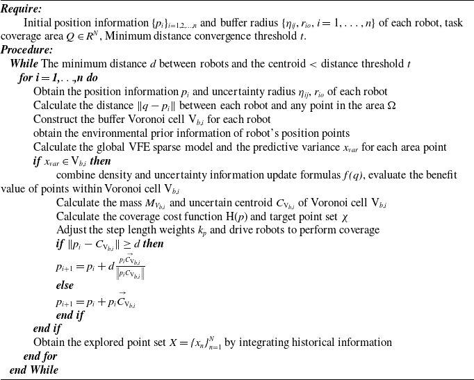
Pseudocode for multi-robot online coverage and source localization

The pseudocode for multi-robot online coverage and target localization algorithm is shown in Algorithm 1.
4. Simulation analysis
This paper verifies the effectiveness of the proposed algorithm through MATLAB 2018a simulation software, setting up two groups of comparative simulation experiments. In order to make the simulation more general, the following designs are implemented:
-
(1) The maximum number of iterations is set to 120 times;
-
(2) The kernel function in the VFE method is the radial basis function;
-
(3) The maximum speed of the robot for each iteration is 1.5 m/s.
4.1. Formation safety verification
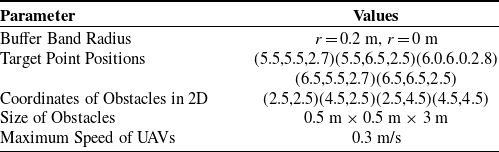
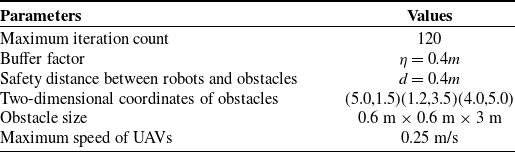
To validate the obstacle avoidance performance of the algorithm, the following experiments were conducted. In this experiment, the simulation environment was set to 7 m × 7 m × 7 m, with five robots and four obstacles. To verify the influence of the buffer width on the formation, we set two different buffer parameters, r = 0 m and r = 0.2 m. By adjusting the width of the buffer zone, changes in the formation performance indicators were observed. Table I shows the experimental parameter settings.
Experimental parameter settings.

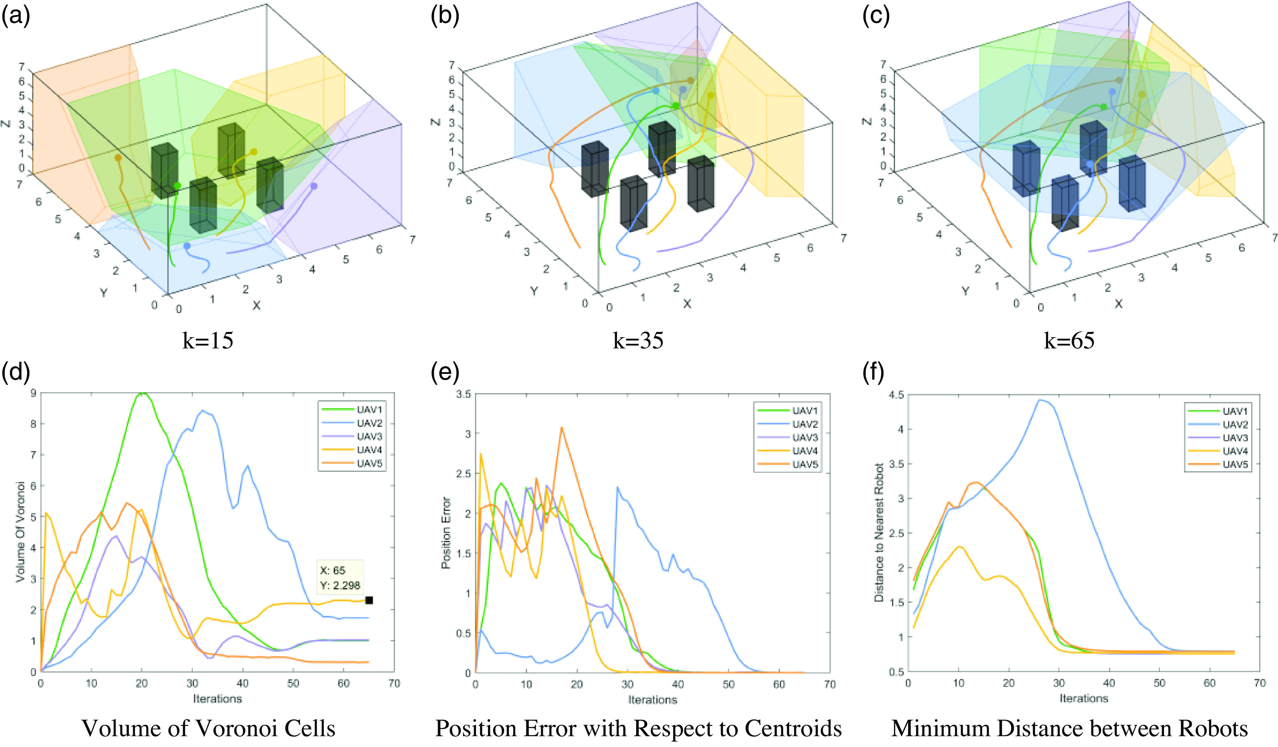
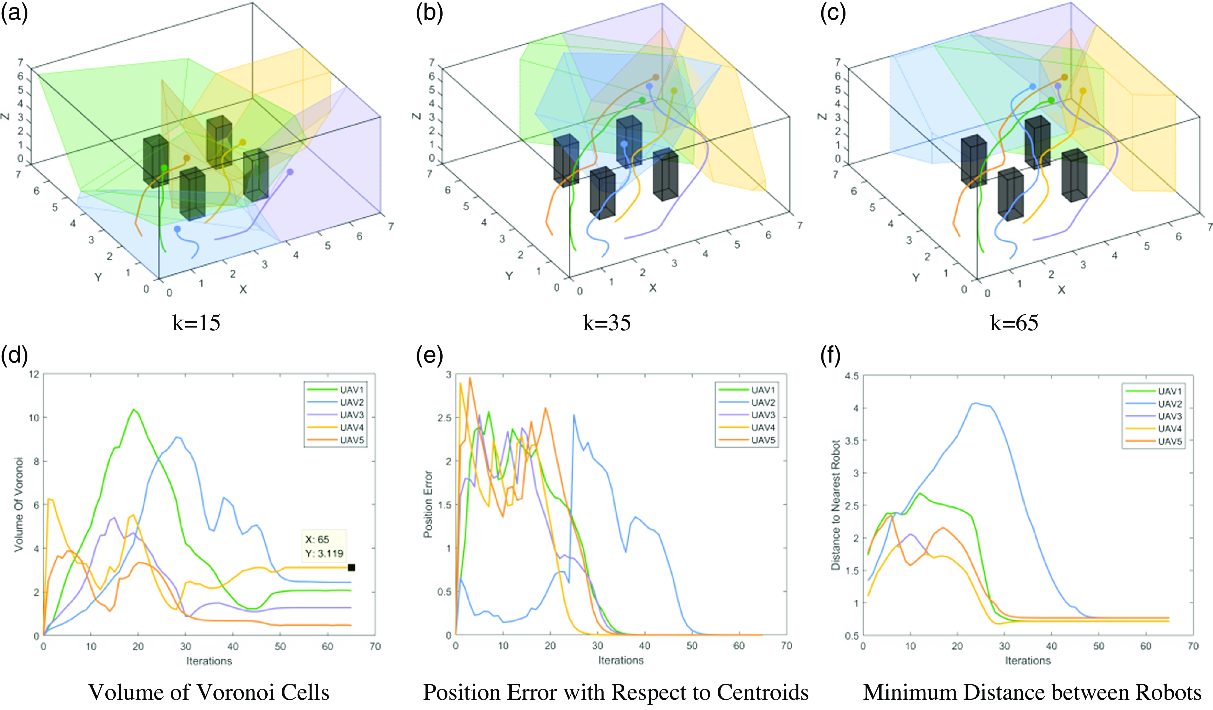
The goal of this experiment is to have five robots reach predetermined locations while avoiding obstacles along the path. Therefore, each robot needs to construct safe Voronoi cells to avoid collisions between robots or between robots and obstacles. The simulation results are shown in Figs. 5 and 6, where in Figure 5(a), (b), and (c), curves of different colors represent the motion trajectories of different robots, and irregular polyhedra represent the Voronoi cells of different robots.
Multi-UAV formation based on buffered Voronoi partition with buffer band radius r = 0.2 m.

Multi-UAV formation based on buffered Voronoi partition with buffer band radius r = 0 m.

It can be observed that all five robots in the experiment are able to avoid obstacles, ensuring the safety of the formation. From Figs. 5(e) and 6(e), it is evident that as the number of iterations increases, the position error between the robots and their target locations decreases, ultimately achieving convergence. Figures 5(d) and 6(d) show that at the end of the iterations, the volume changes of the five Voronoi cells tend to stabilize. The changes in the minimum distance between robots in Figures 5(f) and 6(f) indicate that the minimum distance between the five robots always remains greater than 0.5 m, meaning that there are no collisions between the robots.
From the comparison between the two sets of simulations in Figs. 4(d) and 5(d), it can be seen that at the end of the iterations, the volume of the Voronoi cell generated by UAV2 with a buffer band radius r = 0.2 m is approximately 2.3
 $m^{3}$
, while the volume of the Voronoi cell with r = 0 m is approximately 3.12
 $m^{3}$
. This indicates that as the width of the buffer band increases, the boundaries of the Voronoi cells continuously contract, and the volume of the Voronoi cells decreases. A wider buffer band ensures a smaller Voronoi region that guarantees the robots’ safety. Conversely, a narrower buffer band results in a larger movable safe Voronoi region for the robots.
4.2. Online coverage of multi-pollutant sources
Assuming there are two leakage sources in the coverage area, located at the coordinates (2.5, 2.5, 2.5) and (5.5, 5, 4) respectively, as shown in Figure 2, the actual density function is a compound Gaussian distribution.
 \begin{equation} \rho _{xyz}=5e^{-0\textit{.}5^{\ast}\left[\left(x-2\textit{.}5\right)^{2}+\left(y-2\textit{.}5\right)^{2}+\left(\textit{z}-2\textit{.}5\right)^{2}\right]}+10e^{-0\textit{.}3^{\ast}\left[\left(x-5\textit{.}5\right)^{2}+\left(y-5\right)^{2}+\left(z-4\right)^{2}\right]} \end{equation}
In the simulation environment, the point (5.5, 5, 4) is the location of the maximum concentration. In order to observe the movement trajectory of the robots more conveniently, the number of obstacles has been reduced to 3, while the number of robots remains at 5. Table II shows the experimental parameter settings.
Experimental parameter settings.

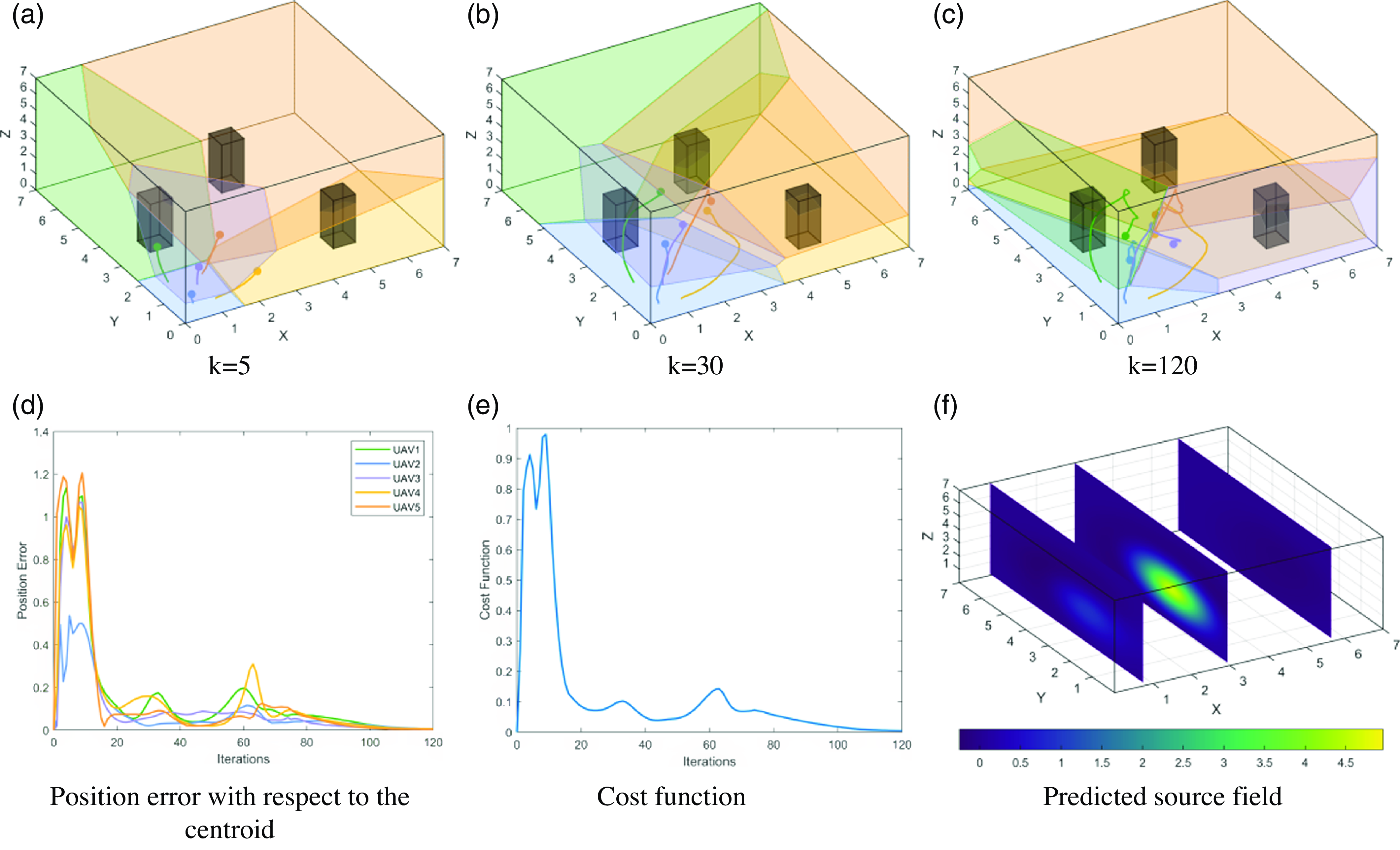
Multi-UAV coverage and source localization process under the GPR-CVT.

The online coverage method using VS-GPR will be compared with the traditional GPR method, and the experimental results are as follows.
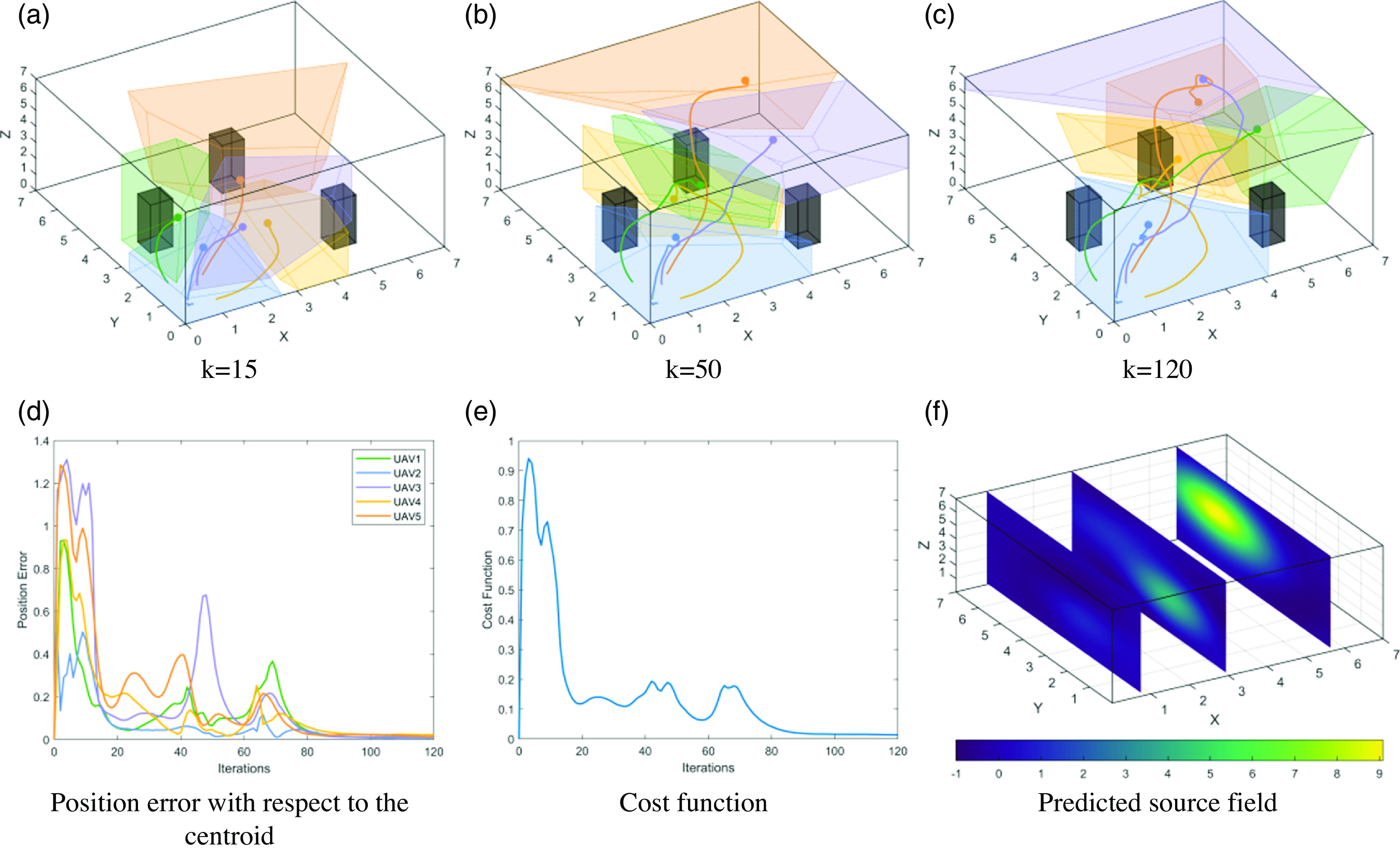
Figures 7(a) to (f) show the simulation results of multi-robot online coverage tasks completed using the GPR-CVT algorithm, while Figure 8(a) to (f) show the results using the SGPR-BCVT algorithm. As can be seen from the simulation in Figure 7(b), the traditional GPR-CVT algorithm may collide with obstacles during movement, resulting in safety problems for the robot. In the subsequent simulation in Figure 7(c), the traditional GPR-CVT algorithm returned after covering a certain distance, and could not accurately cover the location of the pollution source. From Figure 8(a), it can be observed that the SGPR-BCVT algorithm introduces a buffer zone between each Voronoi cell during the initial Voronoi cell generation stage to avoid collisions between robots. In addition, it can be seen from the subsequent simulation Figure 8(b) and (c) that the robot has been moving towards the location of the pollution source, so that the robot can locate the location of the pollution source more accurately in the future. Figures 7(f) and 8(f) respectively depict the concentration prediction maps of leakage sources under the GPR-CVT and SGPR-BCVT algorithms. The traditional GPR-CVT algorithm fails to accurately locate the two pollution sources, while the SGPR-BCVT algorithm can cover more areas and ultimately successfully identify the two different pollution sources.
Multi-UAV coverage and source localization process under the SGPR-BCVT.

4.2.1. Mutual avoidance between robots and obstacles
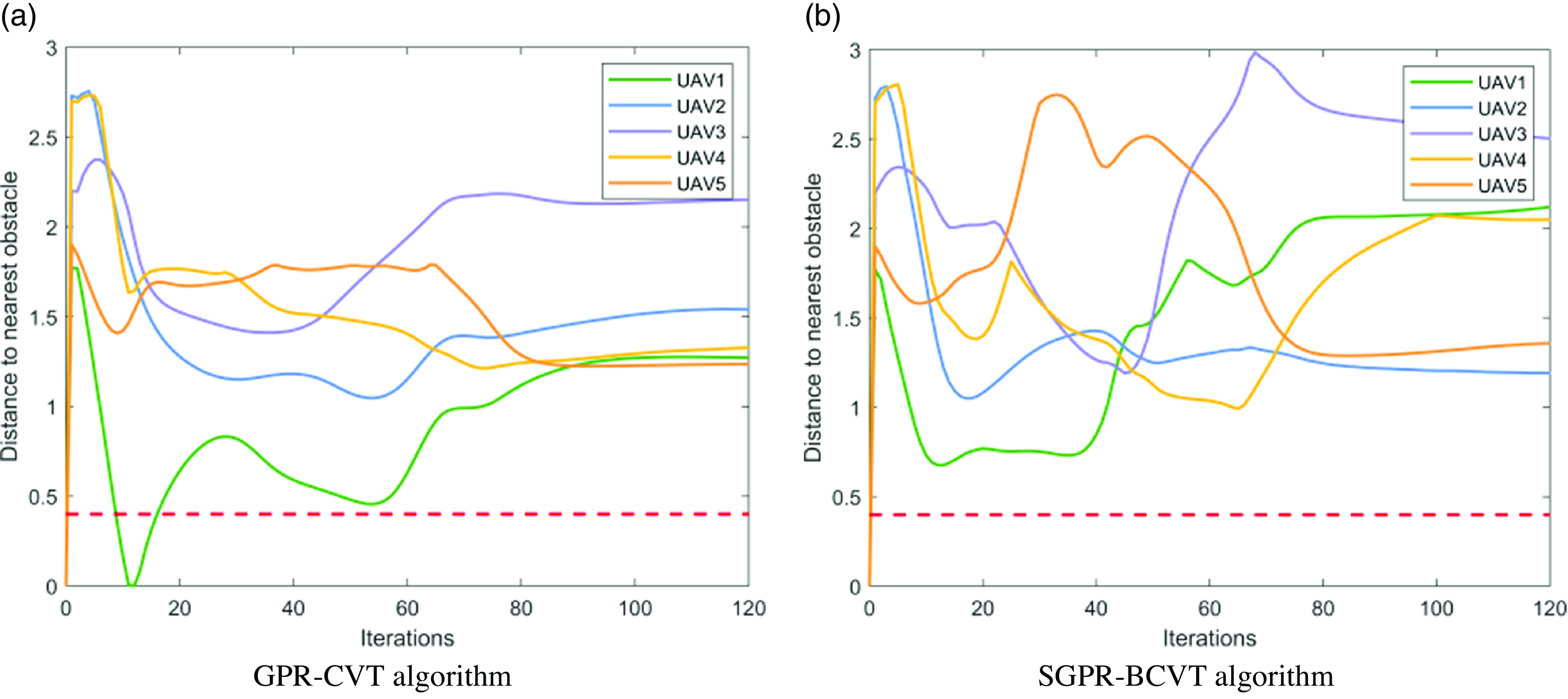
Figure 9 shows the simulation of the minimum distance evaluation index between robots and obstacles. The safe distance between robots and obstacles is set to 0.4m, as indicated by the red dashed line in Figure 9(a) and (b). The distance between UAV1 and the obstacle under the GPR-CVT algorithm is less than the safe distance, indicating a collision. However, Figure 5(b) shows that during the formation process, the distance between any robot and obstacle under the SGPR-BCVT algorithm always remains greater than the safe distance, meaning that the robots can safely complete the formation task.
Minimum distance between UAVs.

4.2.2. Model accuracy performance index
To verify the accuracy of the source field prediction under the proposed algorithm in this paper, the root mean square error is used to evaluate the regression model. Eq. (41) expresses it specifically.
 \begin{equation} RMSE=\sqrt{\frac{1}{m}\sum _{i=1}^{m}\!\left(p\!\left(x_{i}\right)-y_{i}^{\ast}\right)^{2}} \end{equation}
where
 $p(x_{i})$
represents the predicted value obtained using the SGPR model, and
 $y_{i}^{\ast}$
represents the true value of the leakage field.
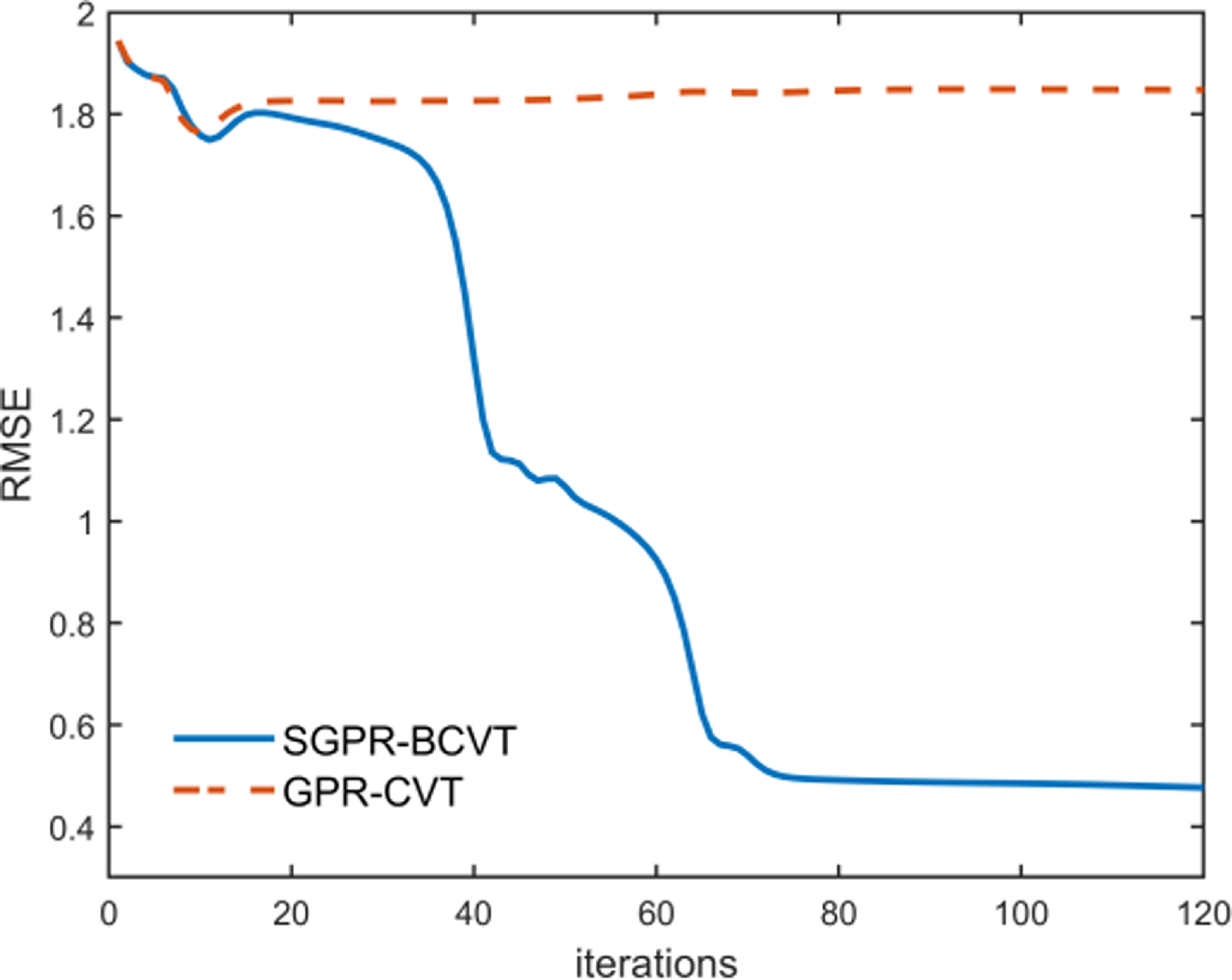
Figure 10 shows the root mean square error of the models established by two algorithms under the source described in Eq. (40). Compared to the real field data, at the end of the iteration, the error of the model established by the SGPR-BCVT algorithm decreased by 75.44%, while due to the GPR-CVT algorithm causing the robot to fall into a local extremum, the model error only decreased by 4.96%. Therefore, in terms of the accuracy index of the established model, the SGPR-BCVT algorithm has a significant advantage.
Model accuracy metrics.

4.2.3. Accuracy of source localization
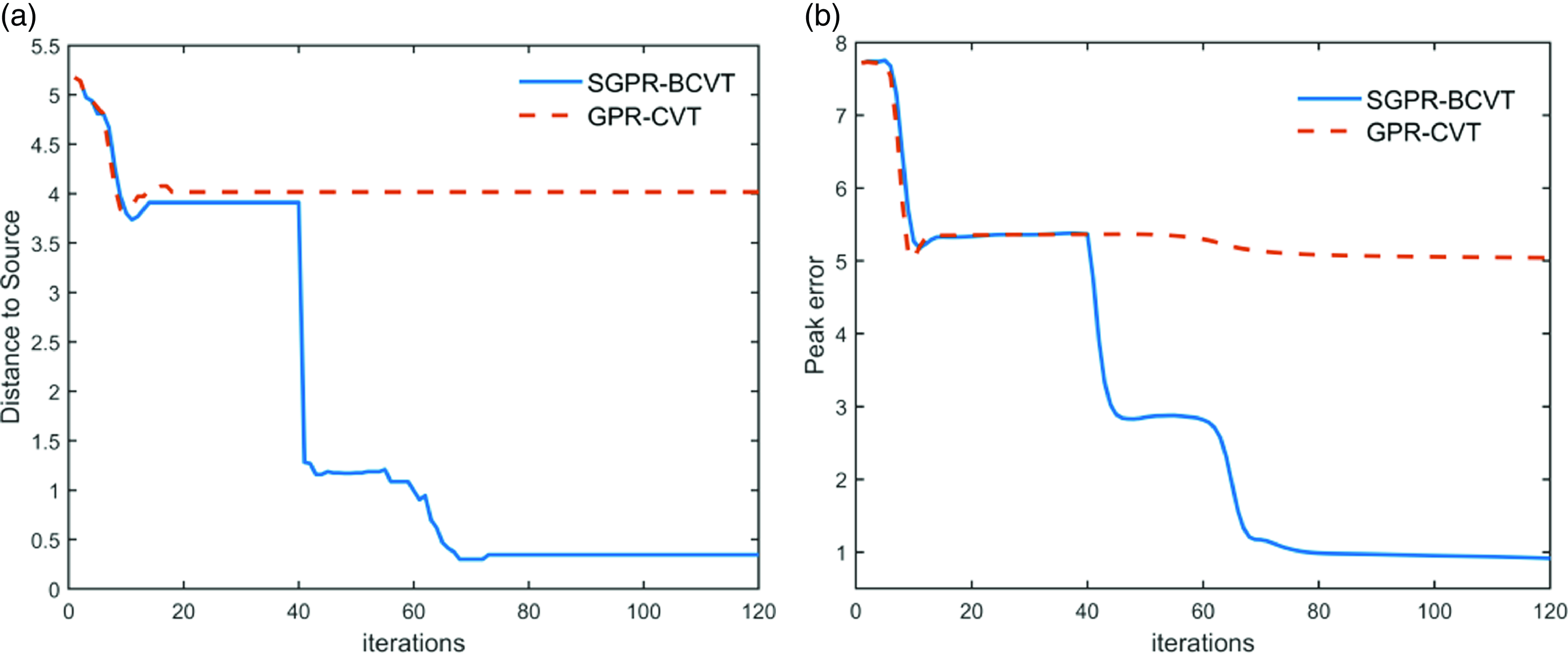
In order to evaluate the accuracy of multiple agents in reconstructing hazardous source fields, two evaluation metrics are proposed: DE (Distance Error) and EE (Extremum Error).
DE: The Distance Error metric calculates the difference in distance between the predicted field and the location of the maximum concentration in the real field;
EE: The Extremum Error metric calculates the difference in concentration between the predicted field and the maximum concentration point in the real field;
The smaller the values of the Distance Error and Extremum Error metrics, the higher the credibility of the established model, and the more precise description of the source field can be achieved.
Figure 11 indicates that the performance of the traditional GPR-CVT algorithm is poor and cannot accurately locate the two pollution sources. In contrast, the algorithm proposed in this paper guides the robot to explore uncertain areas as much as possible. Compared with the real field data, the localization distance and concentration errors of the extremum points are reduced by 93.31% and 88.14%, respectively.
Accuracy metrics for source localization. (a) Concentration error in extremum point localization. (b) Distance error in extremum point localization.

4.2.4. Rapidity of online coverage
The simulation runtime comparison of the two algorithms is shown in Table III. It can be seen that the total iteration time of the SGPR-BCVT algorithm is 272.63 s, with an average single iteration time of 2.27 s, while for GPR-CVT, it is 5.61 s. Compared with the two algorithms, there is little difference in the overall path distance, which further indicates that the proposed SGPR-BCVT algorithm can move roughly the same path distance in a short period of time, and can also ensure the accurate location of the pollution source. However, the traditional GPR-CVT algorithm not only takes a long time and the moving distance is roughly the same but also cannot guarantee the location of the pollution source, which further proves the location effectiveness of our proposed algorithm.
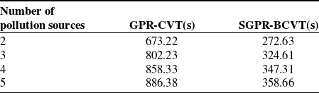
In addition, we also compared the running time of GPR-CVT algorithm and SGPR-BCVT algorithm under multiple pollution sources. As shown in Table IV, the runtime of SGPR-BCVT algorithm for locating two to four pollution sources increased by 19.01\% and 4.99\% respectively, while the running time did not increase significantly when increasing to the five pollution source, which was due to the constraints of spatial scope and the number of robots. It can be seen that with the same number of iterations, the running time of the proposed SGPR-BCVT algorithm is always smaller than that of the GPR-CVT algorithm as the number of pollution sources increases.
Based on the analysis of the simulation results above, it can be concluded that the proposed algorithm can not only reduce the iteration time but also effectively approach the prediction model accuracy of the global Gaussian process regression algorithm under the condition that the whole path is roughly the same. Moreover, when the number of sample points is large, the advantages of this algorithm are more significant.
5. Experiments
To further validate the effectiveness of the online coverage algorithm proposed in this paper in practical scenarios, this section will conduct experiments on the reconstruction and positioning of light sources in the field using Crazyflie drones equipped with light-sensitive sensors. In this experimental environment, the task area is set to a size of 3.2 m × 3.8 m × 1.5 m, and the radius of each drone is 0.05m.
Runtime and overall path distance of two online coverage control algorithms.

Runtime comparison of multiple pollution sources.

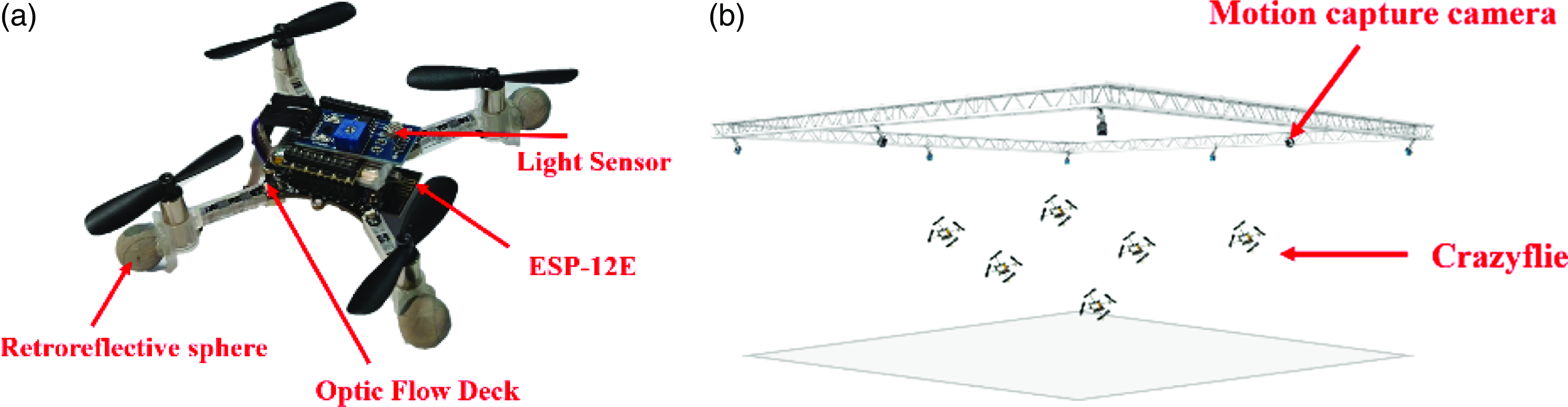
As shown in Figure 12(a), the Crazyflie drones used in the experiment have the capability of sensing light sources. Firstly, the light-sensitive sensor collects data on light sources and sends the data to the base station via the ESP8266-12E module as prior density information input. Additionally, retroreflective ball markers are attached to the Crazyflie drones, and their real-time position information is captured via Optitrack. This information is then sent to the base station via the ROS system as prior positional information input. The light sensor module can change the output voltage according to the ambient light intensity. The input range of analog voltage is 0 to 4096, so the corresponding illuminance level is calculated based on the voltage measured by the sensor. The overall experimental environment is shown in Figure 12(b).
Experimental environment setup. (a) Crazyflie with attached photosensitive sensor. (b) Schematic diagram of multiple Crazyflie formations.

The overall process of the experiment is as follows: After capturing the motion status information of the Crazyflie and the light intensity information at the drone’s current location, the obtained position and field strength information are transmitted to the ROS control terminal. The ROS control terminal analyzes and processes the data through MATLAB-ROS joint programming, ultimately obtaining the distribution of light sources and the next target position of the drone. Finally, the next target position information is sent to the Crazyflie to achieve formation flight of multiple Crazyflie drones.
In the experiment, the gray rectangular area represents the task area. White nets are used around the task environment to ensure flight safety, preventing drones from flying out of the task area and ensuring the safety of flight. The minimum and maximum flight heights of the Crazyflie drones in the experiment are set to 0.5m and 1.5m, respectively.
5.1. Drone formation obstacle avoidance experiment
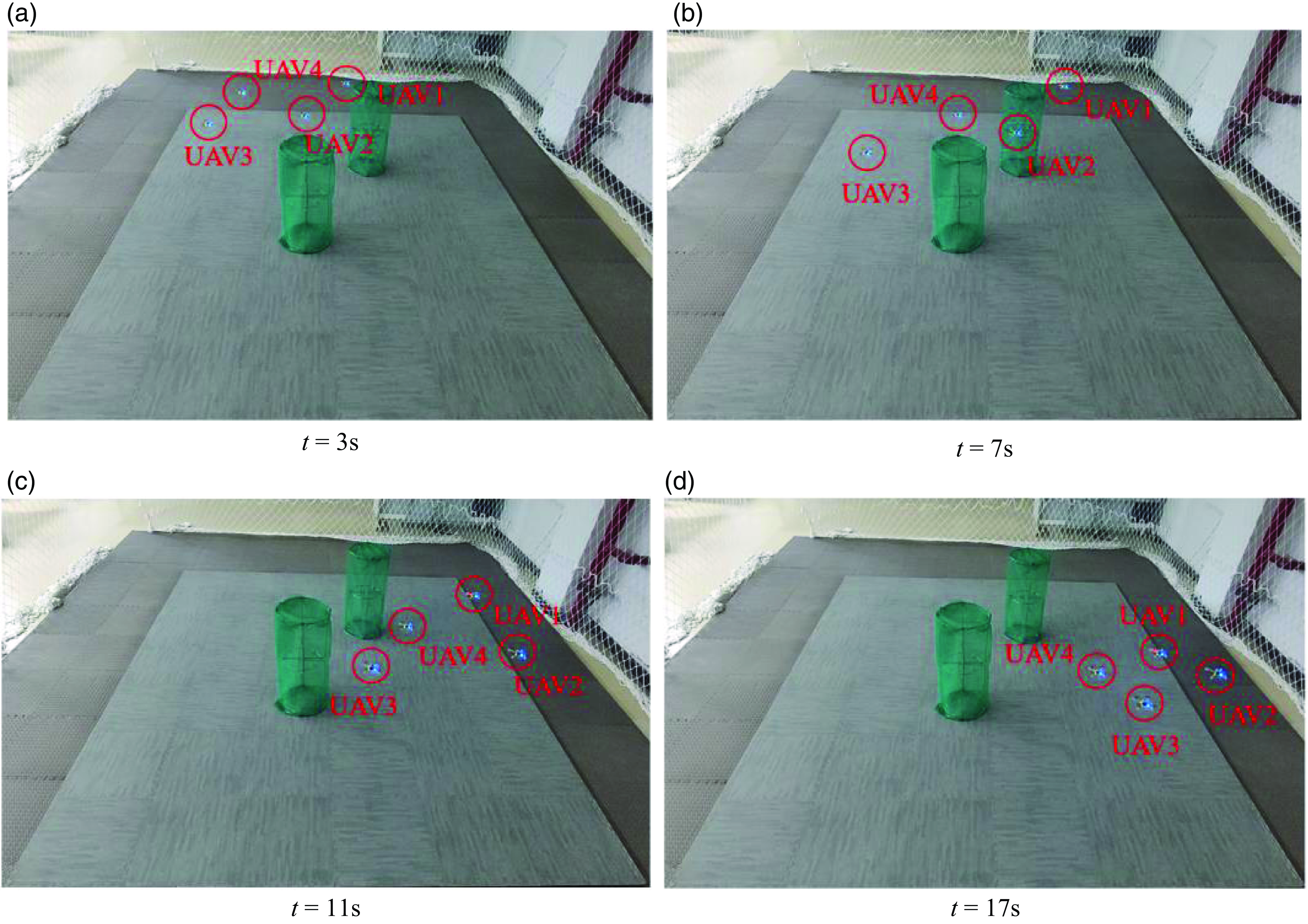
This experiment is designed to validate the feasibility of the formation obstacle avoidance algorithm in a real environment. Two green cylinders represent obstacles located at fixed positions within the task area. The main task of the drones is to fly to four predetermined target points while avoiding obstacles along the way to ensure the safety of the formation. The minimum distance between Crazyflie drones is set to 0.2m, and the minimum distance between drones and obstacles is set to 0.25m. The formation process is illustrated in Figure 13.
Formation safety experiment of four drones.

It can be observed that the 4 Crazyflie drones did not collide with obstacles during the flight and accurately reached the designated target positions after 17 s. The experimental results demonstrate the feasibility of applying the formation obstacle avoidance algorithm to physical drones.
5.2. Drone formation coverage and source localization experiment
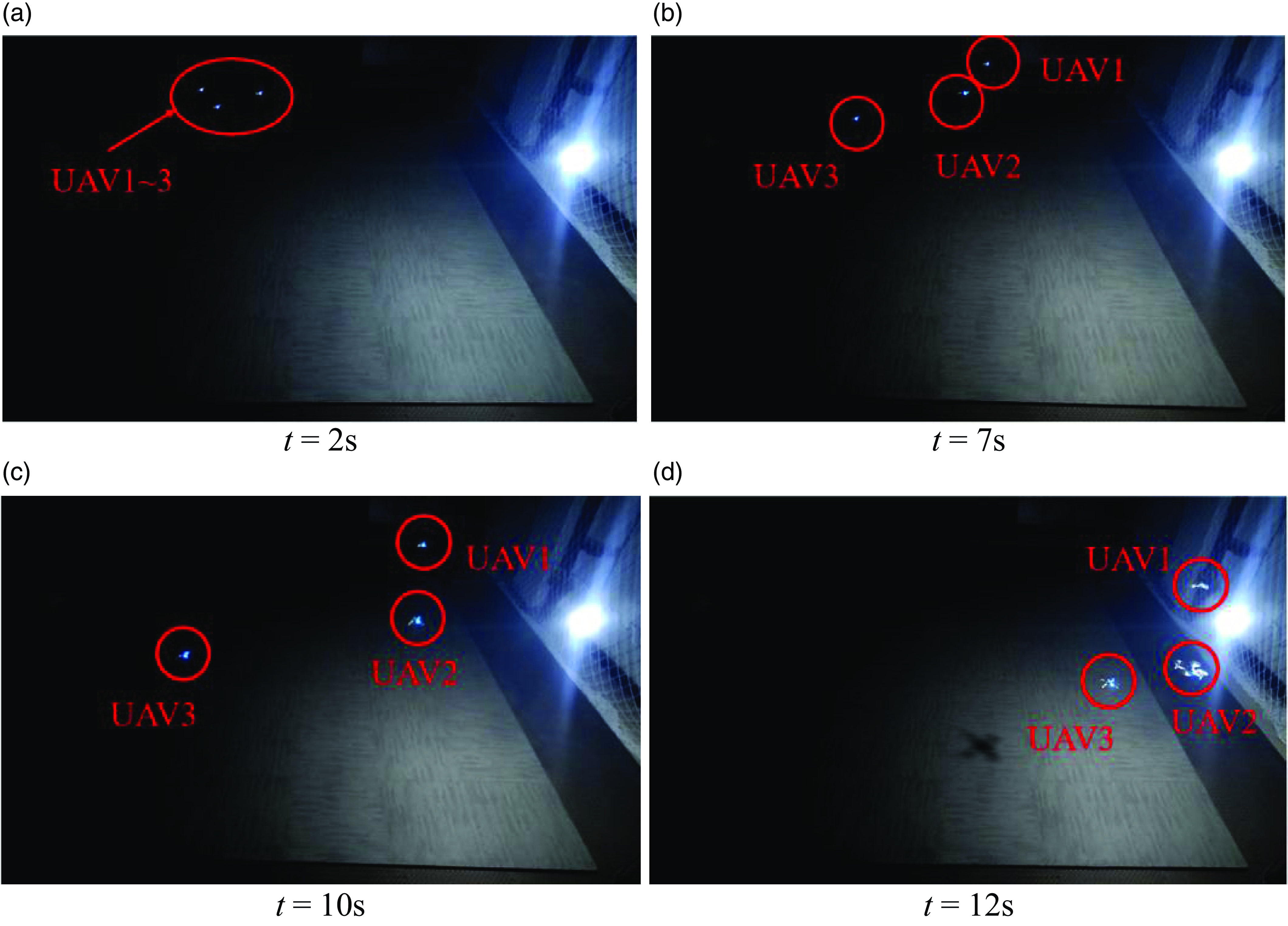
This experiment aims to validate the feasibility of the proposed coverage algorithm in a real environment. In contrast to the previous experiment, this section introduces the use of hanging light bulb sources to simulate pollution sources. In this experimental scenario, the light sources are located in the bottom right corner of the scene, and three Crazyflie drones depart from the top left corner of the map. The light intensity information obtained from light-sensitive sensors and the position information acquired from Optitrack are used as prior inputs to the algorithm. The distribution of the light source field is reconstructed by the movement of drones within the task area, ultimately pinpointing the location of the light source. The experimental process is illustrated in Figure 14.
Formation coverage and source localization of three drones.

It can be seen that in the initial stages, due to the scarcity of light intensity information, the drones may head towards areas with greater uncertainty. However, as the number of available prior sample points increases, the predicted distribution of the field becomes more accurate. At this point, the drones tend to move towards areas where high density and uncertainty are balanced. Ultimately, the drone formation converges, achieving multiple drones’ online coverage and the localization of the light source in the light source environment. Due to the limitation of the scale of the experiment site, the UAV only needs a few iterations to reach the pollution source location, so the total iteration time in the experiment is relatively small. Whether the experimental scenario is simple or complex, the control principle is the same, and eventually the coverage and pollution source will be located.
6. Conclusion
This paper addresses the problem of online coverage and source localization for multiple robots, combining the VS-GPR method with an improved CVT algorithm to achieve efficient coverage and pollution source localization in uncertain environments. The algorithm first considers the potential collisions between robots by adjusting the size of the buffer factor to ensure safety between them and utilizes SVM methods to avoid collisions with obstacles. Secondly, it reduces the time consumption of model training by using the VS-GPR method, effectively improving the exploration and coverage efficiency of multiple robots in unknown field sources while ensuring model accuracy. Subsequent simulations and experiments have confirmed the effectiveness of the proposed algorithm. The characteristics of the leak sources studied in this paper follow a Gaussian distribution, and future research will focus on smoke plume diffusion environments and heterogeneous multi-robot formation studies based on this research.
Author contributions
K.C. and S.G. conceived and designed the study. Y.-B.W. and K.C. conducted code implementation and drone experiments. Y.-Q.C. guided this study. Y.-B.W., K.C., S.-B.Y., and K.Y. wrote this article.
Financial support
This work was financially supported in part by National Natural Science Foundation of China Youth Fund (No.:62103315, 62303368), Ministry of Education Key Laboratory of Information Fusion Technology Open Fund Project (No. 202312-IFTKFKT-007), Shaanxi Province Technical Innovation Guidance Project (No.: 2022QFY01-16), Shaanxi Province Key Industry Innovation Chain Project (No. 2023-ZDLNY-61).
Competing interests
The authors declare no conflicts of interest exist.
Ethical approval
Not applicable.