1. Introduction
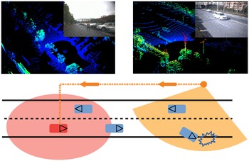
Enhanced 3D perception is a significant ingredient in many state-of-the-art driving systems and vehicle–road-connected systems [Reference Bansal, Krizhevsky and Ogale1, Reference Wang, Devin, Cai, Krahenbuhl and Darrell2]. As shown in Fig. 1, precise 3D object detection is important in both vehicleside and roadside. Object detection serves as a fundamental task for 3D perception and various types of sensors are used in many applications such as monocular images [Reference Simonelli, Bulo, Porzi, Lopez and Kontschieder3, Reference Xu and Chen4], stereo images [Reference Li, Chen and Shen5, Reference Qin, Wang and Lu6], and point cloud from 3D LiDAR [Reference Zhou and Tuzel7, Reference Yan, Mao and Li8]. Compared to image-based detection, point cloud can provide reliable depth information, which is accurate for object localization and shape characterization. However, unlike images, point clouds are sparse and most regions of 3D space are without measurements. In addition, the point density is highly variable due to the factors such as nonuniform sampling of the 3D space, effective range of sensors, occlusion, and the relative motion. Traditional robotics pipeline consists of background subtraction, spatiotemporal clustering, and classification [Reference Leonard, How, Teller, Berger, Campbell, Fiore, Fletcher, Frazzoli, Huang and Karaman9, Reference Himmelsbach, Mueller, Luttel and Wunsche10]. However, the hand-crafted features become a bottleneck of the traditional methods. Hand-crafted features are used to describe objects such as edges, corners/interest points, blobs/regions of interest points, and ridges. With the development of the deep learning trend, more research studies began to explore 3D object detection domain. Thus, this paper proposes a deep learning-based method to detect objects which is an exploration in 3D object detection domain.
Vehicleside and roadside perception illustrations. Top left: it consists of point cloud and image from the ego-vehicle; Top right: it consists of point cloud and image from a road-side infrastructure. Below: the light red circle represents the perception range of the red ego vehicle and the light orange sector represents the perception range of the orange road-side LiDAR. With the vehicle-to-everything (V2X) technology [Reference Tsukada, Oi, Ito, Hirata and Esaki47], the accident information can be transferred to the ego vehicle so it can foresee the road status and avoid the accident.

The key of 3D LiDAR object detection is to represent the sparse and unordered point cloud for subsequent processing. In the past few years, several popular representations were proposed, including Range View [Reference Meyer, Laddha, Kee, Vallespi-Gonzalez and Wellington11], Point View [Reference Shi, Wang and Li12], Bird’s Eye View [Reference Lang, Vora, Caesar, Zhou, Yang and Beijbom13], and fusion of them [Reference Shi, Guo, Jiang, Wang, Shi, Wang and Li14]. Compared to other representations, the object scale and range information were preserved in the BEV representation. However, the representation of BEV was sparse which caused the direct application of convolutional neural networks (CNNs) impractical and inefficient. Recent works such as PointNet [Reference Qi, Su, Mo and Guibas15], VoxelNet [Reference Zhou and Tuzel7] and Sparsely Embedded Convolutional Detection (SECOND) [Reference Yan, Mao and Li8] were trying to apply the end-to-end learning in 3D object detection domain. The drawback of these methods was the slow inference speed because of the 3D convolutions. VoxelNet’s performance was strong but the inference speed was 4.4 Hz which was unable to implement in real-time detection tasks. In order to reduce inference time, PointPillars [Reference Lang, Vora, Caesar, Zhou, Yang and Beijbom13] and multi-view fusion (MVF) [Reference Zhou, Sun, Zhang, Anguelov, Gao, Ouyang and Vasudevan16] used a pillar-like encoder to predict 3D boxes for the objects. Pillar-like encoder was fast because all key operations can be formulated as 2D convolutions which were efficient to compute on a graphics processing unit (GPU). Recently, a cross-stage partial (CSP) network was proposed, which can reduce computation by 20
 $\%$
with equivalent or even superior accuracy on the ImageNet dataset [Reference Wang, Liao, Wu, Chen, Hsieh and Yeh17]. In terms of feature integration, multiscale prediction methods such as feature pyramid network (FPN) [Reference Lin, Dollár, Girshick, He, Hariharan and Belongie18] have become popular due to its light-weighted characteristics. The main motivation is to build a deep neural network for 3D object detection using point cloud and the proposed method should be able to meet the requirements of inference speed and detection accuracy. In general, the ability of real-time performance is related to the sensor frame rate, such as 10 frames per second (fps) for LiDARs and 30 fps for cameras [Reference Arnold, Al-Jarrah, Dianati, Fallah, Oxtoby and Mouzakitis19].
In this paper, a light-weighted deep learning method is proposed to reduce heavy computing and ensure real-time object detection performance in an embedded system. The pillar feature encoding method is used for point cloud representation. A CSP-based 2D CNN backbone and an FPN-based neck are designed to generate a feature map. A multioutput head structure is attached to predict classes, bounding boxes, and orientations of the objects. The main contributions of this paper are as follows:
-
1. A light-weighted deep neural network model is designed for object detection in real time. To reduce computation and ensure accuracy, the CSP and FPN structures are applied according to the characteristic of the point cloud.
-
2. By sharing a convolutional layer, a multioutput head is simplified to predict the classes, the bounding boxes, and the orientations of the objects simultaneously.
-
3. Comprehensive experiments and ablation studies are conducted to evaluate the precision and speed of PLOT. Results show that the PLOT is able to deploy in an embedded system.
This paper is organized as follows: Section 2 reviews the related works on deep learning-based object detection approaches. Section 3 details the proposed method for 3D object detection. Section 4 gives experimental results and a comparison with existing works, followed by the conclusion in Section 5.
2. Related works
Object detection methods using deep learning were well-studied in 2D visual recognition. The general deep learning pipeline involved backbone networks and detection heads. In visual recognition, the input image was passed through a backbone network to learn abstract features, while the detection head predicted the bounding boxes. In 3D point cloud, different considerations were taken to improve the performance due to the sparsity. The related works on object detection using learning-based methods are given below.
2.1. 2D object detection
The pioneer method in 2D object detection task was regions with CNN features (RCNN) [Reference Girshick, Donahue, Darrell and Malik20], a two-stage approach for image recognition. A simple selective search was used to find regions of interest and subsequently applied a CNN to bottom-up the region proposals to regress the parameters of bounding boxes. Fast RCNN [Reference Girshick21] was proposed to solve the problem of RCNN by sharing features for each region proposal from the same image. All the region features were cropped and resized from the shared feature map to improve the inference speed. The Faster RCNN [Reference Ren, He, Girshick and Sun22] was proposed to further improve speed and performance by replacing the selective search of Fast RCNN with a region proposal network. Mask RCNN [Reference He, Gkioxari, Dollár and Girshick23] was built on top of Faster RCNN. A mask prediction module was added to generate a single pipeline that was able to solve tasks such as object detection, semantic segmentation, and instance segmentation. Instead of using region of interest (ROI) pool to resize feature to a fixed grid, a bilinear interpolation method was proposed in mask RCNN to avoid quantization error. Beyond structural changes in the two-stage object detection models, many extensions were used to improve detection performance, such as multiscale information using feature pyramids networks [Reference Lin, Dollár, Girshick, He, Hariharan and Belongie18], deformable convolutions [Reference Dai, Qi, Xiong, Li, Zhang, Hu and Wei24], and iterative refinement of box prediction [Reference Cai and Vasconcelos25].
In addition to two-stage object detection, many object detection models were proposed to solve real-time problems via one-stage algorithms. Single Shot Detector (SSD) [Reference Liu, Anguelov, Erhan, Szegedy, Reed, Fu and Berg26] and You only look once (YOLO) [Reference Redmon, Divvala, Girshick and Farhadi27, Reference Redmon and Farhadi28] were representative examples of one-stage object detection methods. RetinaNet [Reference Lin, Goyal, Girshick, He and Dollár29] was proposed to improve the accuracy and efficiency using a focal loss function in a single stage framework, which can amplify a sparse set of hard examples and prevent easy negativesFootnote 1 from overwhelming the detector during the training. In this paper, a one-stage framework is used to assure the inference speed which is the main requirement for autonomous vehicles. The accuracy rate is improved based on the network design, data augmentation, and other technical strategies.
2.2. 3D object detection
Point cloud are able to provide a natural representation of 3D shapes and scenes. As such, 3D convolutional network was the paradigm of several early works [Reference Engelcke, Rao, Wang, Tong and Posner30, Reference Li31]. The architectures of these methods were straightforward, and the inference speed was slow. In the method Vote3Deep [Reference Engelcke, Rao, Wang, Tong and Posner30], the sparse convolutional layers were used for efficient large-scale processing of 3D data, and the processing time of a single scan of point cloud requires more than 1.1 s on a 4-core 2.5 GHz CPU. PointNet [Reference Qi, Su, Mo and Guibas15] and PointNet++ [Reference Qi, Yi, Su and Guibas32] exemplified a broad class of deep learning method that operates on raw point cloud. They achieved approximately 10 scans per second in the indoor classification dataset such as ModelNet40 and S3DIS. The multilayer perceptron was used to lift points to high-dimensional space, and the symmetric set function was applied to aggregate the features of points. The inference speed of PointNet and PointNet++ is faster than Vote3Deep. Graph neural networks were used in dynamic graph CNN (DGCNN) [Reference Wang, Sun, Liu, Sarma, Bronstein and Solomon33] on the k-nearest neighbor graphs to learn the geometric features of point cloud. The processing time is moderate compared to Vote3Deep and PointNet. The Kernel Point Convolution (KPConv) [Reference Thomas, Qi, Deschaud, Marcotegui, Goulette and Guibas34] was proposed as a new design of point convolution. A set of kernel points was used to define the area where each kernel weight was applied, which was also extended to deformable convolutions that learn to adapt kernel points to local geometry. KPConv was efficient and robust to varying densities. In general, KPConv was faster than all the methods mentioned previously.
With the development of automated driving technology, many experimental vehicles and roadside infrastructures are using 3D LiDAR sensors as an input of environmental perception. Thus, there were increasingly research studies on 3D object detection for autonomous vehicles and roadside infrastructures. A generic one-stage network VoxelNet [Reference Zhou and Tuzel7] was proposed for 3D object detection. The point cloud was voxelized and dense 3D convolutions were used to perform feature learning. To enhance the processing efficiency, ORiented 3D object detection from PIXel-wise neural network predictions (PIXOR) [Reference Yang, Luo and Urtasun35] and PointPillars [Reference Lang, Vora, Caesar, Zhou, Yang and Beijbom13] were proposed to organize point cloud in vertical columns which reduced the amount of input size. MVF [Reference Zhou, Sun, Zhang, Anguelov, Gao, Ouyang and Vasudevan16] was proposed to fuse both BEV pillars and perspective view pillars. Frustum PointNet [Reference Qi, Liu, Wu, Su and Guibas36] was proposed to segment and classify the point cloud in a frustum generated from projecting a detection on an image. The benchmark performance was superior compared to other fusion methods.
However, the multistage design was impractical for end-to-end inferring in real time. SECOND [Reference Yan, Mao and Li8] was proposed to improve the efficiency of VoxelNet, which resulted in stronger performance and an inference speed of 20 Hz. However, the expensive 3D convolutional layers were unable to be removed which made it difficult for edge computing scenarios. A graph neural network [Reference Yin, Shen, Gao, Crandall and Yang37, Reference Yin, Shen, Guan, Zhou and Yang38] was proposed to enhance the detection precision by using spatiotemporal transformer attention. Another one-stage method [Reference Li, Zhao, Zhao, Zhang and Shen39] was proposed for 3D vehicle detection which applied an anchor-free head to improve the calculation efficiency. As the ground truth labels were significant for model training, the weakly supervised framework [Reference Meng, Wang, Zhou, Shen, Jia and Van Gool40, Reference Meng, Wang, Zhou, Shen, Van Gool and Dai41] was studied to train a neural network model using few samples. The previous works explored many directions for different object detection tasks. In general, two-stage frameworks such as Fast R-CNN, Mask R-CNN can reach the highest accuracy rates, but are typically slower. As for one-stage framework such as YOLO, SSD, they treat object detection as a simple regression problem by taking an input image and learning the class probabilities and bounding box coordinates. Such models reach lower accuracy rates, but are much faster than two-stage object detectors. In this paper, our priority is real-time 3D object detection, thus we value inference speed more than accuracy. Some of the reviewed works are categorizing in Table I.
Method comparison table.

3. Proposed method
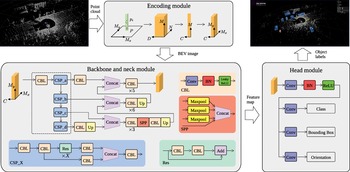
The proposed PLOT framework is shown in Fig. 2. The original input is the point cloud and the final output are the 3D bounding boxes of the estimated entities. Three main stages are listed: (1) a point cloud encoding structure that converts a point cloud to a pillar-based BEV image; (2) a multilayer convolutional backbone to transform the BEV image into high-dimensional representations; (3) a detection head to predict the classes and orientations and regress the 3D bounding boxes.
Framework overview. The three stages of the network (encoding module, backbone module, and head module) are illustrated using grey boxes and the workflow is denoted by the arrows. The detailed description is given in Section 3. The raw point cloud is converted to a pillar-based gird map. The encoding module is used to encode the grid map into a multichannel BEV through a CNN. A CSP-based backbone with neck is applied to extract the high dimensional features, and a multioutput head is attached to predict the classes, bounding boxes, and orientations of objects.

3.1. Point cloud encoding
With the unordered and scattered point cloud as input, the first step is to convert them into a pillar-based BEV image. As shown in Fig. 2, the whole points in a point cloud are denoted as
 $P$
, and each point in
 $P$
is denoted as
 $p(x,y,z,I)$
, which contains the position in Cartesian coordinate system and the intensity.
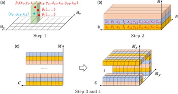
As shown in Fig. 3(a), the x–y plane is discretized into an evenly spaced grid with the width
 $M_x$
and the length
 $M_y$
. The center of each grid is denoted as
 $(x_c,y_c,z_c)$
, and
 $z_c$
is calculated based on the maximum height parameter which is determined in the experiment section. For each point in a grid, the offsets are defined as
 $x_o=|x-x_c|$
,
 $y_o=|y-y_c|$
,
 $z_o=|z-z_c|$
. Then, all the points in detection range are represented as follows:
 \begin{equation*} \hat {p}(x,y,z,I,x_c,y_c,z_c,x_o,y_o,z_o) \end{equation*}
where
 $\hat{p}$
has a dimension
 $D=10$
. The dimension is easy to be expanded when more information on points, such as ambient and reflectivity is provided.
Illustrations of point cloud encoding step 1 and step 2. In (a), green pillar denotes a grid, red dots represent the scattered points and blue dot is the center of a grid. In (b), each color (pink, blue, yellow) denotes a grid, each slice in a grid denotes a point with
 $D$
elements. In (c), each color represents a grid with
 $C$
elements.

Then, as shown in Fig. 3(b), points in each grid are combined as a
 $N \times D$
block, and all the nonempty grids are then stacked as a tensor of size
 $(M,N,D)$
. Note that the number of points in each grid is not the same,
 $N$
is set to be the maximum number. The points are randomly sampled when the number in a grid exceeds
 $N$
, and zeros will be padded to fill the points. A convolution layer with Batch Normalization (BN) and Rectified Linear Unit (ReLU) is applied to encode the input into a
 $(M,N,C)$
tensor. A maximum pooling layer is applied to calculate the maximum value in
 $N$
points. As shown in Fig. 3(c), the output tensor size is
 $(M,C)$
in step 3 and the features are then scattered back to the original grid location in step 4. Finally, a multichannel BEV of size
 $(M_x,M_y,C)$
is created for the network backbone.
3.2. Backbone and neck
In order to guarantee the real-time object detection ability, a multilayer backbone and a neck are designed according to YOLOv4 [Reference Wang, Bochkovskiy and Liao42]. YOLOv4 is a one-stage object detection model that improves on previous YOLO models with several bags of tricks and modules such as CSP, Mish activation. It was designed to run on general GPUs which was able to deploy in edge computing scenarios. The main purpose of using CSP structure is to achieve a richer gradient combination while reducing the amount of computation. This aim is achieved by partitioning feature map of the base layer into two parts and then merging them through a cross-stage hierarchy. The gradient flow propagated through different network paths by splitting the gradient flow [Reference Wang, Liao, Wu, Chen, Hsieh and Yeh17]. The whole backbone structure is illustrated in Fig. 2. The input is a tensor with size
 $(M_x,M_y,C)$
. Firstly, a convolution layer with BN and leaky ReLU is used to encode the input tensor into higher dimension. Then four CSP modules (CSP_a, CSP_b, CSP_c, CSP_d) are connected one by one to downsample the tensor at a stride
 $S$
. Each CSP module consists of five CBL modules and n Res modules and the Res module is inserted to achieve the effect of gradient stunting. Finally, four tensors from CSP modules are achieved in the backbone part.
The neck part is designed based on the FPN, which mainly integrates the features coming from different feature pyramids. FPN [Reference Lin, Dollár, Girshick, He, Hariharan and Belongie18] is a top-down architecture with lateral connections developed for building high-level semantic feature maps at all scales. In this paper, four outputs from the CSP modules are concatenated with upsampling process. Firstly, the output of the CSP_d module in the bottom is upsampled through a CBL module and a Up module to fit the tensor size of the CSP_c output. Then a spatial pyramid pooling (SPP) module is applied to map multiple size input down to a fixed-size output. In this paper, the SPP module contains three maximum pooling layers and is inserted between two CBL modules. Three concatenating modules are used to connect the outputs from backbone step by step and finally a feature map is generated for the head module. The details of implementation will be discussed in Section 4.
3.3. Detection head
The detection head is a neural network layer attached to the neck. Based on the feature map extracted by the backbone and neck, the head is designed to perform actual task, such as detection and segmentation. In this paper, a multioutput head is designed based on the region proposal network [Reference Girshick21, Reference Ren, He, Girshick and Sun22] to predict classes, bounding boxes, and orientations of the objects. First, a CNN followed by BN and ReLU is used as a sharing convolutional layer for the three types of predictions to reduce computation. Then three separate convolutional layers are applied to fit the configuration of each type of predictions. The channels are designed based on the number and rotation of anchors. For the bounding box prediction, the 3D Intersection over Union (IoU) is used to calculate the relative loss to the ground truth which is more precise than the 2D IoU used in PointPillars [Reference Lang, Vora, Caesar, Zhou, Yang and Beijbom13].
3.4. Loss function
The loss function is used to map the inferring results onto the ground truth. In this paper, three different loss functions are proposed to measure the difference between the head output and the ground truth. Due to the unbalanced amounts of generated anchors and label positive ground truth objects, the loss function of type classification is defined based on the focal loss [Reference Lin, Goyal, Girshick, He and Dollár29]:
 \begin{equation} \mathcal{L}_c = -{\alpha _c}(1-p_c)^{\gamma _c}\log{p_c} \end{equation}
where
 $p_c$
is the classification probability of the anchor. The parameters
 $\alpha _c$
and
 $\gamma _c$
are 0.25 and 2.0 according to the original paper settings.
The ground truth of the bounding box and anchors are defined by
 $(x,y,z,d_x,d_y,d_z,\theta )$
, representing the coordinates of the center point and the length, width, height, and orientation of the object. The residuals of localization regression are defined as follows:
 \begin{equation} \begin{cases}{\Delta }x &= (x^{\text{gt}}-x^{\text{p}})/d_{x}^{\text{gt}}\\[5pt] {\Delta }y &= (y^{\text{gt}}-y^{\text{p}})/d_{y}^{\text{gt}}\\[5pt] {\Delta }z &= (z^{\text{gt}}-z^{\text{p}})/d_{z}^{\text{gt}}\\[5pt] {\Delta }d_x &= \log{(d_{x}^{\text{gt}}/d_{x}^{\text{p}})}\\[5pt] {\Delta }d_y &= \log{(d_{y}^{\text{gt}}/d_{y}^{\text{p}})}\\[5pt] {\Delta }d_z &= \log{(d_{z}^{\text{gt}}/d_{z}^{\text{p}})}\\[5pt] {\Delta }\theta &= \sin{(\theta ^{\text{gt}} - \theta ^{\text{p}})}\\[5pt] \end{cases} \end{equation}
where superscript
 $^{\text{gt}}$
represents the ground truth and
 $^{\text{p}}$
is the prediction results per anchor. The loss function of the bounding box prediction is defined based on the weighted smooth L1 loss [Reference Yan, Mao and Li8]:
 \begin{equation} \mathcal{L}_b = \sum _{t \in (x,y,z,d_x,d_y,d_z,\theta )}{\text{SmoothL1}(\Delta t)} \end{equation}
and the angle loss can only represent the intersection without direction, so an orientation prediction is added in this paper. The orientation loss
 $\mathcal{L}_{o}$
is defined by a softmax classification function. The final loss function consists of three parts:
 \begin{equation} \mathcal{L} = \omega _c \mathcal{L}_c + \omega _b \mathcal{L}_b + \omega _o \mathcal{L}_o \end{equation}
where
 $\omega _c = 1.0$
,
 $\omega _b = 2.0$
and
 $\omega _o = 0.2$
are the constant weights of losses.
4. Experiments
In this section, the implementation details are given, including dataset details, network settings, and data augmentation (DA). Then a quantitative experiment is carried out to compare the results of the proposed method to other state-of-the-art methods. Real-time experiments in different scenarios are designed to test the edge computing ability of the proposed method. Ablation studies are conducted to demonstrate the effectiveness of the whole network architecture.
4.1. Implementation details
4.1.1. Dataset
The Waymo Open Dataset [43] is used in this paper to train and test the proposed method. The dataset contains 798 training sequences with 158,361 LiDAR scans and 202 validation sequences for the entities. The point cloud is captured with a 64-line LiDAR scanner sensor, which returns about 180,000 points in 0.1 s. The official 3D detection evaluation metrics consists of the standard 3D bounding box mean average precision (mAP) and mean average precision weighted by Heading (mAPH). The mAP and mAPH are calculated based on an IoU threshold of 0.7 for vehicles, 0.5 for pedestrians, and cyclists. A performance breakdown for two difficulty levels is provided in the official evaluation toolkit: Level 1 (L1) for boxes more than 5 LiDAR points and Level 2 (L2) for boxes with at least 1 point.
4.1.2. Network settings
The detection range is set according to the Waymo dataset, the range of X and Y axis is
 $[\!-\!74.88, 74.88]$
m, and the range of Z axis is
 $[\!-\!2, 4]$
m. The resolution of a grid is set as 0.32 m in both X and Y axis, which is enough to distinguish small objects. The maximum number of points in one grid is set to 32 according to the point cloud distribution. In the encoding module, the kernel size of the convolutional layer is
 $1 \times 1$
and the channel number is 64. After encoding, the output tensor size is
 $468 \times 468 \times 64$
.
In the backbone and neck module, the parameters
 $(a,b,c,d)$
are first determined by our experience. The main idea is to keep the network small and efficient, which requires less CSP modules. On the other hand, the input is downsampled to extract more high-dimensional features. The first CSP module uses 1 Res module (
 $a=1$
) and the stride is set to 1, the output tensor is
 $468 \times 468 \times 64$
. Then the parameters
 $b=1$
,
 $c=d=3$
are applied with
 $S=2$
and the output tensors of the three CSP modules are
 $234 \times 234 \times 128$
,
 $127 \times 127 \times 256$
and
 $64 \times 64 \times 512$
. The neck part upsampled the tensors from
 $64 \times 64 \times 512$
to
 $468 \times 468 \times 64$
. The shared weight convolutional layer has 64 channels, and three anchor-based head layers are defined as follows:
Vehicles: the anchors with length, width, and height are set as
 $(4.73,2.08,1.77)$
and
$(9.60,2.30,2.70)$
for small cars and large trucks. The bottom height of the anchors is 0, and the positive and negative matching thresholds are 0.55 and 0.4.
Pedestrians and cyclists: the anchors with length, width, and height are set as
$(0.91,0.84,1.74)$
and
$(1.81,0.84,1.77)$
. The bottom height of the anchors is 0, and the positive and negative matching thresholds are 0.5 and 0.3.


The proposed detector is trained using stochastic gradient descent with an Adam onecycle optimizer running on four NVIDIA GTX 2080Ti GPUs. All models are trained for 150 epochs and the initial learning rate is 0.0001, with an exponential decay every 15 epochs with a factor 0.8.
4.1.3. Data augmentation
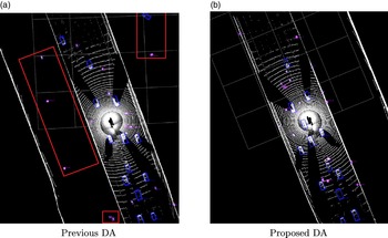
The major problem of the dataset is the low ratio of ground truths to outlier points. To solve this problem, the SECOND [Reference Yan, Mao and Li8] proposed a DA method that randomly put objects from other scans into the current scan, which can increase the number of ground truth in one scan. However, the randomly placed objects are unable to fit in the environment (such as a car is isolated in the middle of nowhere), which leads to the problem that the inserted ground truth has no geometry constraints. In this paper, the ground truths are inserted in the road which is extracted first. The difference between the previous method and the proposed method is shown in Fig. 4.
Data augmentation comparison. All ground truths are placed in the road area to keep the geometry constraints. The red boxes in (a) denotes the objects generated outside the road using previous DA method.

In the proposed DA method, all the ground truth boxes are rotated randomly in
 $[\!-\!\pi/ 20, \pi/ 20]$
range of angle. Then, the boxes are translated randomly following a uniform translation distribution, the mean and standard deviation of the distribution are 0 and 0.25. In addition, a random scaling and rotation are applied to the whole point cloud in one scan. The scaling range is from 0.95 to 1.05, and the rotation range is
 $[\!-\!\pi/ 4, \pi/ 4]$
.
4.2. Experiment results
The quantitative and qualitative analysis are conducted to demonstrate the effectiveness of the proposed method.
4.2.1. Quantitative evaluation
The quantitative evaluation experiment is conducted based on the Waymo dataset using the official evaluation detection metrics. PLOT is compared to three state-of-the-art detection methods: PointPillars [Reference Lang, Vora, Caesar, Zhou, Yang and Beijbom13], SECOND [Reference Yan, Mao and Li8], and Point Voxel RCNN (PV-RCNN) [Reference Shi, Guo, Jiang, Wang, Shi, Wang and Li14]. PointPillars, SECOND, and PLOT are one-stage detection methods that are fast for real-time tasks. PV-RCNN is a two-stage detection method requiring heavy computing in the proposal refine part.
The results are shown in Tables II, III and IV. All three compared methods are trained and tested with the same data as PLOT. Compared to the one-stage methods, PLOT achieves similar precision to SECOND in vehicle and cyclist detection and higher precision in pedestrian detection. There are three downsampling steps in PointPillars so it is difficult to detect small targets such as pedestrians and cyclists even with data augmentation. PV-RCNN achieves the highest precision in vehicle and cyclist detection. With the highest precision in pedestrian detection, PLOT is unable to provide an accurate heading angle for pedestrian. However, the inference time of PV-RCNN is around 150 ms running on a GTX 2080Ti GPU.
Vehicle detection results.

Pedestrian detection results.

Cyclist detection results.

In order to deploy the detection method on real-time tasks shown in Fig. 1, the intelligent computing hardware is a NVIDIA Jetson Xavier NX developer kit that brings super-computer performance to the edge [44]. The device delivers up to 21 TOPS for running modern AI workloads and consumes 10 W of power. The width and length of the device are around 10 cm and the height is 8 cm, which is suitable for deployment in a car or a roadside box. In general, the desktop GPUs such as RTX 3090 has 20 times AI workloads than NX but also requires 20 times more power consumption, which is not suitable for autonomous vehicle nor roadside. With 21 TOPS computing resources, it is difficult to keep two-stage methods running in real time. Thus, only one-stage methods are deployed into the device using TensorRT tools [45].
The real-time experiment is conducted using an Ouster OS1-128 LiDAR scanner mounted on top of a vehicle. The point cloud data is processed in real time and recorded for analysis. The dataset contains 20 min driving (about 20,000 scans) in the city area. Three individual devices are equipped on the vehicle to run the detection method at the same time. The results of the real-time experiment are shown in Table V. The evaluation settings are the same as in Waymo dataset; only the mAP in L1 is listed.
Real-time experiment results.

1 AIT means average inference time for each model.
2 The PLOT is trained using DeepRoute open dataset.
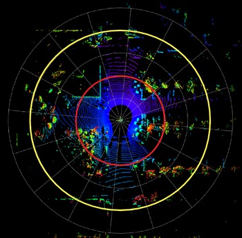
Detection range of the OS1-128 LiDAR sensor. The indent of grey circles is 10 m. The red circle denotes 20 m and the yellow circle represents 40 m from the sensor.

The PLOT outperforms two other methods in vehicle and cyclist detection. The average precision of pedestrian and cyclist is lower than the results in the Waymo dataset. One main reason is that the city road has six lanes with guardrail to separate the nonmotorized vehicle lane, which makes the pedestrian and cyclist difficult to be scanned. Another reason is that there are many electric bicycles which is not included in the Waymo dataset. One possible way to solve this problem is to label the electric bicycles to enlarge the training dataset. With the help of a new proposed open dataset from DeepRoute [46], more cyclist samples are added to the training dataset. The PLOT model is retrained using 10,000 scans of point cloud data and all the parameters remain the same. The detection results are denoted in Table V, and the mAP of the cyclist is about 38% higher than the original PLOT model trained using Waymo dataset. The results of vehicle and pedestrian are also improved. However, there are still some false negative results that may affect the autonomous vehicle’s decision making. The frequency of the LiDAR sensor is 10 Hz which requires an inference time less than 100 ms. With the CSP-based backbone and FPN-based head, the average inference time of the PLOT is around 46 ms, which is faster than the other two methods.
According to the detection range of the OS1-128 LiDAR scanner, we divided the range into three parts, as shown in Fig. 5. We evaluate the detection mAP in each range section to analysis the detection ability of the proposed method, and the results are shown in Table VI. In the red circle with the range less than 20 m, the mAPs of vehicle, pedestrian, and cyclist are over 90%, 70%, and 60%, which is able to be used as an auxiliary warning system in the roadside scenarios and low-speed autonomous driving scenarios. In addition, due to the sparsity of point cloud, it is difficult to extract the objects over 40 m from the sensor, which caused the low mAPs in Table VI.
Detailed results.

1 The PLOT is trained using DeepRoute open dataset.
2 Inf means infinity.
4.2.2. Qualitative evaluation
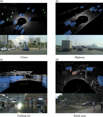
After the evaluation of average precision in two datasets, more experiments in different scenarios are carried out. The results are shown in Fig. 6. Four scenarios are tested, including urban road, highway, underground parking lot, and rural areas. A camera is mounted in front of the vehicle to capture videos while driving. There are more electric bicycles in the urban scenario which are shown in purple, as shown in Fig. 6(a). The trucks and cars are not distinguished and are marked in blue as shown in Fig. 6(b). The pedestrian in the underground parking lot can be detected in 30 m which is capable to meet the requirements in Auto Valet Parking system. The predictions for vehicles are accurate and common failure modes include false negatives on difficult samples such as partially occluded objects. In some cases, electric bicycles are misclassified as vehicles because they have large cargo in the back (delivery bicycles). Additionally, pedestrians are easily confused with narrow vertical features such as small trees and poles. Thus, the detection results require further processing with the help of other sensors such as cameras and radars.
Performance under different scenarios. Point cloud and front image are displayed. The vehicles are labeled in blue, pedestrian in orange, and cyclists in purple.

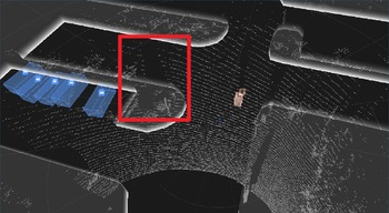
In addition, the proposed method is applied in a roadside perception node. The Ouster OS1-128 LiDAR sensor is mounted on top of a road sign pole with the height 4.2 m. With a simple coordinate transformation procedure, the PLOT is fitted into the roadside scenario. The result is shown in Fig. 7, with the fixed position of the LiDAR sensor, and the ROI can be easily set by adding virtual wall. The ROI area can eliminate most of the false positive detections such as poles and trees outside the road. One advantage of object detection is the less occlusion of the entities, and the point cloud is able to return more points from an object. On the other hand, when the LiDAR sensor is blocked by a tree like the red box area in the figure, the occlusion will be large and may lead to some false negative results.
Road side scenario. The white edges represents a virtual wall of the ROI, blue boxes denotes the vehicles, and orange box is a pedestrian. The red box area denotes an occlusion caused by a tree.

4.3. Ablation studies
In this section, extensive ablation experiments are carried out to analyze individual components of the proposed method. All models are trained and evaluated in the same data in the Waymo dataset. Note that the average precision represents the mAP in L1.
4.3.1. Point cloud encoding
In point cloud encoding module, the number of output channels and the activation function are related to the final accuracy and inference speed. Table VII shows the comparing results. The inference time is 15% faster when the number of output channels is halved but the average precision is more than 10% lower. The results of different activation function are similar which indicates that the effect of activation function is not obvious.
4.3.2. Backbone and neck
Table VIII demonstrates the results of different backbone and neck structures. Note that all the parameters are set to be the same as Section 4.1.2 and the learning epoch is set to be 150. The first structure is used in YOLOv4 [Reference Wang, Bochkovskiy and Liao42] and path aggregation network (PAN) represents path aggregation network which is equipped as the neck part. The number after CSP represents the number of CSP modules and the number of residual blocks in each CSP module. For example, CSP [1,2] means there are two CSP modules, the first CSP module contains one residual module and the second CSP module contains two residual modules.
In the image processing domain, the input image with a large size needs to be downsampled multiple times to extract the features of small objects. However, in point cloud detection domain, the input of point cloud is sparse and the size of objects remains the same in different range from the sensor. As the results show, the precision increases when the number of CSP modules decreases. In addition, the PAN module is usually used to fuse the features from different size which is not suitable in point cloud processing. The average precision is increased when the PAN is removed.
4.3.3. Detection head and data augmentation
For detection head comparison, the SSD-based detection head used in PointPillars [Reference Lang, Vora, Caesar, Zhou, Yang and Beijbom13] is applied. The results are shown in Table IX. The average precision of the entities are 62.44, 53.21, and 47.28. In addition, the SSD structure is more complex than the head of PLOT. As for the effects of the proposed data augmentation method, a new PLOT model is trained with the data without data augmentation. The average precision of the entities are 65.76, 58.62, and 51.23. It can be seen that with the data augmentation, the precision of small objects is improved by more than 5%. The precision of vehicle detection is slightly improved because most of the samples are already on the road.
Point cloud encoding comparison results.

Backbone and neck comparison results.

Detection head and data augmentation results.

5. Conclusion
In this paper, a 3D point cloud object detection (PLOT) network is proposed to reduce heavy computation and ensure real-time performance in an embedded system.Footnote 2 A pillar feature encoding method is proposed to convert the sparse point cloud into BEV image. A backbone using CSP-based structure is applied to downsample the input tensor and an FPN-based neck is designed to generate a feature map. Finally, a multihead structure is attached to predict the classes, bounding boxes, and orientations of the objects. The average precision on Waymo dataset is over 60% which outperforms the state-of-the-art methods using one-stage structure. The real-time capability is ensured with an average inference time 50 ms in an embedded system.
Author contributions
Yihuan designed the study. Liang conducted data gathering. Yifan and Liang performed statistical analyses. Yihuan, Liang, and Yifan wrote the article.
Financial support
This work was supported in part by the Natural Science Foundation of Jiangsu Province under Contract BK20200271 and Suzhou Science and Technology Project under Contract SYG202014.
Conflicts of interest
The authors declare no competing interests.