




No CrossRef data available.
Article contents
- Extract
- ESCUDERO AND BOERSMA'S (2004) LISTENING EXPERIMENT
- MEASURING RELATIVE CUE WEIGHTING AS AN EDGE DIFFERENCE RATIO
- THE ALLEGEDLY DETRIMENTAL CEILING EFFECT
- MEASURING RELIANCE FROM THE EDGE: IS LOGISTIC REGRESSION BETTER?
- TAKING ALL DATA INTO ACCOUNT, OR ONLY PART OF THE DATA
- HAS TWO-CATEGORY ASSIMILATION BEEN CONFIRMED?
- GROUPING
- CONCLUSION
- References
MEASURING RELATIVE CUE WEIGHTING: A Reply to Morrison
Published online by Cambridge University Press: 25 October 2005
Article contents
- Extract
- ESCUDERO AND BOERSMA'S (2004) LISTENING EXPERIMENT
- MEASURING RELATIVE CUE WEIGHTING AS AN EDGE DIFFERENCE RATIO
- THE ALLEGEDLY DETRIMENTAL CEILING EFFECT
- MEASURING RELIANCE FROM THE EDGE: IS LOGISTIC REGRESSION BETTER?
- TAKING ALL DATA INTO ACCOUNT, OR ONLY PART OF THE DATA
- HAS TWO-CATEGORY ASSIMILATION BEEN CONFIRMED?
- GROUPING
- CONCLUSION
- References
Extract
Morrison (this issue) criticized the analytical and statistical methods that Escudero and Boersma (2004) used for assessing the participants' cue weightings in their listening experiments. He proposed that logistic regression constitutes a better method for measuring perceptual cue weighting than Escudero and Boersma's “edge difference ratio.” The present paper starts by summarizing and illustrating Escudero and Boersma's experiment and analysis method and then addresses five of Morrison's objections—namely the alleged ceiling effect, the alleged superiority of logistic regression, the problem of discarding data, the (dis)confirmation of two-category assimilation, and Escudero and Boersma's grouping of the data. We will argue that although logistic regression is a very good method for measuring cue weighting, there was nothing wrong with Escudero and Boersma's methodology in these five respects.
Information
- Type
- RESPONSES
- Information
- Copyright
- © 2005 Cambridge University Press
Morrison (this issue) criticized the analytical and statistical methods that Escudero and Boersma (2004) used for assessing the participants' cue weightings in their listening experiments. He proposed that logistic regression constitutes a better method for measuring perceptual cue weighting than Escudero and Boersma's “edge difference ratio.” The present paper starts by summarizing and illustrating Escudero and Boersma's experiment and analysis method and then addresses five of Morrison's objections—namely the alleged ceiling effect, the alleged superiority of logistic regression, the problem of discarding data, the (dis)confirmation of two-category assimilation, and Escudero and Boersma's grouping of the data. We will argue that although logistic regression is a very good method for measuring cue weighting, there was nothing wrong with Escudero and Boersma's methodology in these five respects.
ESCUDERO AND BOERSMA'S (2004) LISTENING EXPERIMENT
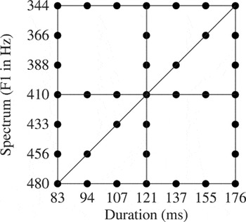
In their listening experiments, Escudero and Boersma (2004) presented the participants with 37 different stimuli, shown schematically in Figure 1. The stimuli were synthesized vowel-like sounds that varied in duration (seven possible values) as well as in spectral quality (seven possible values).

Stimulus set used by Escudero and Boersma (2004).
In the experiment, each of the stimuli was presented 10 times. The 370 trials were presented in a randomized order. The participants' task was to decide whether the vowel they heard was the English /i/ (by clicking on a picture of a sheep) or the English /i/ (by clicking on a picture of a ship). For Southern British English participants, stimuli that were long and had a low F1—the stimuli in the top-right corner of the figure—tended to be classified as /i/, whereas stimuli that were short and had a high F1—those in the bottom-left corner—tended to be classified as /i/; these listeners can thus be said to rely on both the duration cue and the spectral cue. Scottish English listeners were different in that they tended to ignore the duration cue: For them, stimuli in the top half of the figure tended to be classified as /i/ and those in the bottom half as /i/. Spanish learners of English were again different: Some acted like the Scots, some like the Southerners, and some showed a pattern not found in either of the native groups—namely ignoring the spectral cue and classifying the stimuli in the right half of the figure as /i/ and those in the left half as /i/.
In reality, the results were much more variable than just presented. To make sense of the data, we decided to derive from each participant a single quantity—namely the relative extent to which she relied on the two cues.
MEASURING RELATIVE CUE WEIGHTING AS AN EDGE DIFFERENCE RATIO
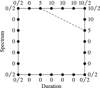
The single quantity that Escudero and Boersma (2004) used for measuring each participant's relative reliance on duration and spectrum was the slope of a reconstructed boundary line, which is a straight line through Figure 1 that best separates the area where the participant predominantly responds /i/ from the area where she predominantly responds /i/. Figure 2 shows how this slope can be computed for an idealized listener, for whom stimuli not on the boundary line are unambiguous.

Measuring the slope from the responses on the edges (ideal listener).
Figure 2 shows how a certain idealized listener responds to 10 replications of each of the 24 possible stimuli on the edge. The dashed line shows the boundary line for this listener. Stimuli in the top right are always heard as /i/, and hence score 10 /i/ responses and 0 /i/ responses; stimuli to its bottom left are always heard as /i/, and hence score 0 /i/ responses (and 10 /i/ responses); the two stimuli that happen to lie on the boundary line score 5 /i/ and 5 /i/ responses.
For the ideal listener in Figure 2, the slope of the boundary line can be computed by two methods. First, it can be computed directly from the line itself. When going 4 units to the right, the line goes down by 2 units, so its slope is (−2)/4 = −0.5. Another way of saying this is that this listener relies on spectrum twice as much as on duration, so that her duration/spectrum reliance ratio is 2/4 = 0.5. However, the slope can also be computed indirectly from the responses along the edges. Along the right edge, there are 60 responses in total (of the 10 measurements in the top-right corner, 5 count with the right edge, 5 with the top edge).1
For Escudero and Boersma (2004), who ignored this corner correction, there were 70 responses along each edge.
Real listeners do not show the 0s, 5s, and 10s of Figure 2 and will have a much more variable pattern so that their boundary line cannot be drawn by simply looking at the numbers around the edges. Therefore, the direct method for computing the slope cannot be used, but an estimate of the slope (and the reliance ratio) can still be computed by the second method—that of dividing the right-left difference by the top-bottom difference—and that is what Escudero and Boersma (2004) did for the participants in their experiments.
THE ALLEGEDLY DETRIMENTAL CEILING EFFECT
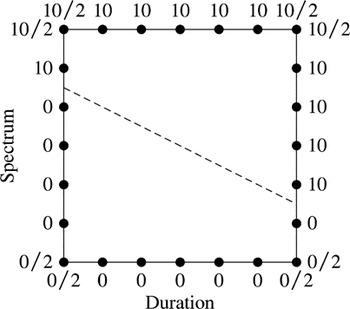
In his critique, Morrison (this issue) mentioned the word ceiling 19 times. In Figure 3, we can see what he meant with this term. The figure shows the boundary line of a second idealized listener. The boundary is in a different location from that of the first listener (see Figure 2), but its slope is identical (again −0.5, because six steps to the right is three steps down); thus its duration/spectrum reliance ratio is also identical (0.5). The duration reliance is computed as 45 /i/ responses on the right edge minus 15 /i/ responses on the left edge, divided by 60, which gives (45 − 15)/60 = 50%. The spectral reliance is 60 /i/ responses along the top minus 0 /i/ responses along the bottom, divided by 60, which gives 100%. It is this 100% value to which Morrison objects: A spectral reliance can never be greater than 100%, so if one finds a spectral reliance of 100% in a specific case, the value is at ceiling and no meaningful measurements can allegedly be based on it. On computing reliance ratios from a spectral reliance that is at ceiling—as in Figure 3—Morrison asserted that “some of the ratios are based on spectral reliances that were at ceiling, and it is not conceptually valid to compare these with ratios based on spectral and duration reliances that were not at ceiling” (p. 603).

Measuring the slope from the responses on the edges (ideal listener with ceiling effect).
Nevertheless, let us compute the ratio as in the previous section—in other words, as if the method were valid after all. The reliance ratio is then computed as 50% divided by 100%, which yields 0.5—the correct value (namely the slope). This perhaps slightly counterintuitive result generalizes to all thinkable cases of boundary lines that intersect the stimulus rectangle: The slope and the reliance ratio can always be correctly estimated as a ratio of response differences, regardless of whether one of the intermediate reliances is at ceiling. It simply works. Morrison's (this issue) assertion is therefore incorrect.
However, Morrison (this issue) made more claims about ceiling effects. He argued that the two so-called cue reliances are ill-defined as observable quantities. This is correct and can be used as a criticism against the use of these quantities as experimental end results by Bohn (1995) and Flege, Bohn, and Jang (1997). For Escudero and Boersma (2004), however, these quantities were nothing more than intermediate values for computing a single reliance ratio, which is the only experimental end result that they discussed. It is only a coincidence that the quantities that Escudero and Boersma needed as intermediate results have the same formal definition as the quantities that Bohn and Flege et al. regarded as experimental results. It is simply possible that a ratio of two ill-defined quantities is a well-defined quantity. We return to this subject in the section “Has Two-Category Assimilation Been Confirmed?”.
MEASURING RELIANCE FROM THE EDGE: IS LOGISTIC REGRESSION BETTER?
Now that the ceiling effect has been shown not to exist for the only relevant measure of relative cue weighting—namely the reliance ratio—it becomes interesting to see whether measures other than Escudero and Boersma's (2004) edge difference ratio could work better.
To demonstrate that logistic regression works better than difference ratios, Morrison (this issue) gives theoretical arguments and pictures of boxplots of Escudero and Boersma's (2004) data. However, the quality of the two procedures can be assessed directly by measuring their performance on known underlying distributions, and that is what we do in this section.
We generated 500,000 different probability distributions for perceiving /i/ that were based on bivariate Gaussian distributions for /i/ and /i/. Each of these 500,000 distributions comes with its own known reliance ratio.2
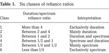
For each of the 500,000 simulations, we started with separate response distributions P(/i/) and P(/i/). For simplicity, we took the duration continuum to run from 1 (left) to 7 (right), and the spectral continuum from 1 (bottom) to 7 (top). The centers of P(/i/) and P(/i/) were connected by a line with a rising slope that was logarithmically evenly distributed between 1/16 (almost horizontal: listeners almost exclusively use the duration contrast) and 16 (almost vertical: listeners almost exclusively use the spectral contrast). The horizontal as well as the vertical position of the midpoint between the centers of P(/i/) and P(/i/) was uniformly distributed between 2.5 and 5.5. The distance between the centers of P(/i/) and P(/i/) was uniformly distributed between 2.4 and 4.8. The standard deviations of duration (σdur) and spectrum (σspec) were uniformly distributed between 0.6 and 2.4. The standard deviations were the same for /i/ and for /i/. As a result, the locations where P(/i/) and P/i/) are equal form a straight line through the figure (the equal-likelihood line). The probability of responding /i/ at a certain point can now be computed as P(/i/)/(P(/i/) + P(/i/), and the boundary line will fall together with the equal-likelihood line. The known duration/spectrum reliance ratio can be computed as the inverse of the slope of the line that connects the centers of P(/i/) and P(/i/), multiplied by the square of the ratio σspec/σdur.
Six classes of reliance ratios

From the generated distributions, the probability that each of the 24 stimuli along the edge of the stimulus rectangle is perceived as /i/ is also known. We can thus simulate a listener with 240 responses along the edge: Each of these 24 probabilities can be used 10 times for computing whether a listener responds /i/ or /i/, so that each of the 24 cells along the edge will end up with a number between 0 and 10. The question now is: How accurate are the two methods in estimating the reliance ratio from the observed response frequencies? For each of the 500,000 simulations, the real underlying class is known from the known reliance ratio. If a method that estimates the reliance ratio from the simulated responses ends up classifying the reliance ratio in a different class, we consider this an error.
The edge difference ratio method used by Escudero and Boersma (2004) turned out to classify 87.5% of the 500,000 simulated listeners into the correct reliance class. The 12.5% of errors all consisted of classifying a listener into an adjacent class. The logistic regression method proposed by Morrison (this issue), applied to the 24 edge points, classified 87.9% of the listeners correctly.3
Logistic and linear regressions were measured with the Praat program (Boersma & Weenink, 2005).
Whereas the two methods under discussion score almost equally well, several other methods turn out to fare worse. The edge difference ratio method on transformed fractions does not work well: For near-logit-transformed fractions
4The 0.01 added to the numerator and denominator is meant to handle fractions of 0 and 1.

)—which equalize the sizes of the frequentist confidence intervals for binomially distributed data, it scores 86.5%. The worst results are found with linear regression, confirming Morrison's (this issue) verdict on this method: For nontransformed fractions, linear regression scores 82.8%; for near-logit-transformed fractions (which are sometimes used to stand in for true logistic regression!), it scores 82.8% as well; for arcsine-transformed fractions, it scores 83.4%.
The result of the simulations for the edge points is that the edge difference ratio is nearly as good as logistic regression. To see a reliable difference between the two methods would require an experiment with 100,000 participants.
TAKING ALL DATA INTO ACCOUNT, OR ONLY PART OF THE DATA
Another possible problem that Morrison (this issue) noticed is the fact that Escudero and Boersma (2004) used only a part of the experimental results. In Figure 1, we can see that every listener had to respond to 37 different stimuli, whereas in Figures 2 and 3, we can see that only 24 of these were used for computing the reliance ratio. Therefore, Escudero and Boersma discarded approximately one-third of the data.5
Morrison (this issue) even claimed that Escudero and Boersma (2004) use only 14 of the 37 stimuli for the measurement of each reliance, but this is irrelevant given that—as argued earlier—the reliance ratio is the only end result and 24 scores are used to compute it.
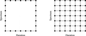
More interesting than the question of whether Escudero and Boersma (2004) should or should not have taken those 13 stimuli into account is the more general question of whether the reliance ratio can be computed better on the basis of the scores on the 24 edge points or on the basis of all 49 possible grid points. Figure 4 shows the two setups.

Two different stimulus sets: edge (left) and grid (right).
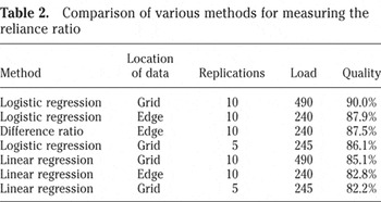
From the previous section, we know that the reliance ratio can be classified correctly from the 24 edge points in 87.5% of the cases (edge difference ratio) or in 87.9% of the cases (logistic regression). For a test of the measurements from all 49 grid points, we have to distinguish 2 cases. The first case is that in which the listener responds 10 times to each of the 49 points. The logistic regression method—when applied to 500,000 simulated listeners—classifies the reliance ratios correctly in 90.0% of the cases, which is better than either of the measurements based on the edges alone. However, the burden on the participants (490 responses) is more than twice as large as when only the edges are measured (240 responses). To equalize the load on the participants, we consider a second case in which the listener only has to respond 5 times to each stimulus, for a total of 245 responses for the whole grid. In this second case, the logistic regression method classifies the reliance ratio correctly for only 86.1% of 500,000 simulated listeners. It thus turns out that if the load for the participants is fixed, it is better to elicit data on the edges (if they do not introduce learning effects) than to elicit data on the whole grid. Table 2 summarizes the results.
Comparison of various methods for measuring the reliance ratio

To sum up, we have shown that linear regression is worse than the other methods (by 4–5%), that measuring the edge alone is better than measuring the whole grid (by 1.8%), and that logistic regression is better than the difference ratio (by 0.4%). As a final note, we mention that Escudero and Boersma's (2004) score would have increased from 87.5% to 89.0% if they had included all of the 37 points of Figure 1 in a logistic regression measurement.
HAS TWO-CATEGORY ASSIMILATION BEEN CONFIRMED?
One of Escudero and Boersma's (2004) proposals was that first language (L1)-Spanish, second language (L2)-Scottish English listeners tend to assimilate the English /i/–/i/ contrast to their native /e/–/i/ contrast and that, hence, they distinguish Scottish English /i/ and /i/ on the basis of spectral differences alone. This proposal was based on the experimental finding that the duration/spectrum reliance ratios of these listeners were approximately zero: Given that the nonbeginners identify “ship” and “sheep” correctly without additional training, they must have been able to somehow perceive the contrast, and given that they cannot rely on duration, they must have relied on the spectral cues. Morrison (this issue) challenged this proposal on the basis of his finding that a comparison of the spectrum-tuned logistic regression coefficients of the various groups shows that these listeners used the spectral cues less than did the native Scottish English listeners and that the difference in spectral cue use between the L2-Scottish English and the L2-Southern English listeners was not statistically significant.
Morrison's challenge does not hold up. First, a failure to reach significance can never deny the existence of a difference. Thus, the only fact that remains is that the L2 Scots used spectral cues less reliably than the native Scots. However, the spectrum-tuned coefficient (βspec) by itself does not tell us why, because it will be low if the listener relies more on duration than on spectrum (a steep slope in Figures 1, 2, or 3), and it will be low if the listener's /i/–/i/ boundary is fuzzy. The former possibility is ruled out by the zero duration reliance, and so the boundary must be fuzzy.
One should not draw too many conclusions on the basis of the degree of crispness of the /i/–/i/ boundary. A fuzzy boundary can be caused by many factors, including nonperceptual ones, and it seems to be a general property of L2 learners that they perform on a lower level than native speakers on almost any task. This is why Escudero and Boersma (2004)—as opposed to Bohn (1995), Flege et al. (1997), and Morrison (this issue)—stayed away from confounded single-dimensional measures of spectral and durational cue reliance and only considered the ratio of these reliances, a measure based on both dimensions together. When measured by reliance ratios, the difference between the L2-Scottish English and the L2-Southern English listeners was indeed significant, and no other explanation than two-category assimilation is available.
GROUPING
As illustrated in the section “Measuring Reliance from the Edge: Is Logistic Regression Better?” Escudero and Boersma (2004) divided the reliance ratios into six classes. As Morrison (this issue) noted, the dividing points (4, 2, 1, 1/2, 1/4) between these classes are arbitrary; this is due to the fact that the range of the horizontal (duration) axis cannot be equated to the range of the vertical (spectrum) axis. However, in fact, Escudero and Boersma's experimental results are likely to be valid only for the stimulus rectangle in Figure 1 because listeners tend to adapt to the size of the rectangle (the range effect; Keating, Mikoś, & Ganong, 1981). This means that boundary locations and orientations tend to depend on the stimulus set (this is one of the reasons why production and perception data are difficult to compare numerically; see Escudero & Boersma, 2003, p. 83); thus, experiment-free division points are out of reach if the stimulus range and the response categories have to be the same for every group of listeners regardless of language background.
Morrison's (this issue) main criticism on the grouping of reliance ratios into classes was that:
[I]f one has a set of data with one value per participant, the normal and straightforward procedure is to run a test based on that set of data—not to divide the data into subgroups and then conduct a test. Dividing the participants into groups reduced the sample size (e.g., from 20 to 6 for each L1-English group), which is likely to result in a less powerful test. (p. 603)
The specific critique of sample size mentioned by Morrison is incorrect: The sample size is still 20. Nevertheless, a direct test on the data is indeed generally preferable. However, a parametric test is inappropriate here because the data are not Normally distributed. But a nonparametric ranked data test is also inappropriate because much of the data is at ceiling: Although Escudero and Boersma's Table 2 (2004, p. 561) orders the subjects by reliance ratio, the ordering in the middle regions—where the ratios are between 0.2 and 5—is much more reliable than the ordering at the edges. For instance, at the edges, we find seven “exclusively duration” participants whose relative ordering must be due to chance. The grouping that Escudero and Boersma performed was one way of making sure that all of these subjects end up effectively unordered. The reason that other possible ways were not considered is that it is plausible that much of the observed data in fact reflects underlying groupings: Many listeners will have a reliance ratio that is essentially zero or infinite because they use a single cue.6
Logistic regression would not help here because it suffers from the same grouping effects.
CONCLUSION
Nearly all of Morrison's (this issue) criticisms to Escudero and Boersma (2004) are based on the implicit assumption that the listening experiment should lead to separate conclusions for durational cue reliance and spectral cue reliance. However, we think that one should be cautious in using such single-dimensional quantities as experimental results, as Bohn (1995) and Flege et al. (1997) did with their edge differences (the measures were referred to as temporal effect and spectral effect in these studies) and Morrison did with the logistic regression coefficients βdur and βspec. This is because these quantities tend to be confounded with factors that make L2 learners perform worse than native speakers on almost any task. Instead, the ratio of these coefficients (i.e., the edge difference ratio, or βdur/βspec) is a measure of relative cue weighting that is intended to maximally cancel out these factors.
Once it is acknowledged that the reliance ratio is the only relevant quantity, the question is how it is to be measured. If prior beliefs about biases in the distributions (such as a belief that reliance ratios cannot be negative) can be ignored, logistic regression is the theoretically optimal method (at least for response distributions based on two Gaussian distributions, as in the simulations presented here). With its minute simulated performance lag of 0.4%, Escudero and Boersma's (2004) edge difference ratio will also be an acceptable method for experiments with less than 100,000 participants; its advantage is that it can be computed by hand. However, if one has measured responses on stimuli inside the rectangle—perhaps because one is afraid of bimodal distribution adaptation effects—logistic regression is the only sensible method capable of taking these responses into account. However, a result of our simulations that is perhaps surprising is that if one is not afraid of bimodal effects, it turns out to be slightly better to collect n responses along the edge than to collect n responses distributed over the whole grid.
We thank Morrison for pointing out the virtues of logistic regression and we will certainly use this method in future analyses. However, we will employ it not for preventing a ceiling effect or for producing single-dimensional reliance measures, but for computing boundary locations and slopes for experiments designed to elicit responses for stimuli on the whole grid as well as for experiments with natural stimuli, whose spectral and durational properties do not have discrete distributions.
References
REFERENCES
Boersma, P., &
Weenink, D.
(2005).
Praat: Doing phonetics by computer (Version 4.3.10)
[Computer program].
Available: http://www.praat.org. Retrieved 25 April
2005.
Bohn, O.-S.
(1995).
Cross language speech perception in adults: First language transfer
doesn't tell it all. In
W. Strange (Ed.),
Speech perception and linguistic experience: Theoretical and
methodological issues (pp.
279–304).
Timonium, MD:
York Press.
Escudero, P.
(2001).
The role of the input in the development of L1 and L2 sound
contrasts: Language-specific cue weighting for vowels. In
A. H.-J. Do,
L. Dominguez, &
A. Johansen (Eds.),
Proceedings of the 25th annual Boston University Conference on
Language Development (pp.
250–261).
Somerville, MA:
Cascadilla Press.
Escudero, P., &
Boersma, P.
(2003).
Modelling the perceptual development of phonological contrasts with
Optimality Theory and the Gradual Learning Algorithm. In
S. Arunachalam,
E. Kaiser, &
A. Williams (Eds.),
Proceedings of the 25th annual Penn Linguistics Colloquium, Penn
Working Papers in Linguistics, 8.1 (pp.
71–85).
Philadelphia:
Penn Linguistics Club.
Escudero, P., &
Boersma, P.
(2004).
Bridging the gap between L2 speech perception research and
phonological theory.
Studies in Second Language Acquisition,
26,
551–585.Google Scholar
Flege, J. E.,
Bohn, O.-S., &
Jang, S.
(1997).
Effects of experience on nonnative speakers' production and
perception of English vowels.
Journal of Phonetics,
25,
437–470.Google Scholar
Keating, P.,
Mikoś, M. J., &
Ganong, W. F., III
(1981).
A cross-language study of range of voice onset time in the
perception of initial stop voicing.
Journal of the Acoustical Society of America,
70,
1261–1271.Google Scholar
Maye, J., &
Gerken, L. A.
(2000).
Learning phoneme categories without minimal pairs. In
S. C. Howell,
S.A. Fish, &
T. Keith-Lucas (Eds.),
Proceedings of the 24th annual Boston University Conference on
Language Development (pp.
522–533).
Somerville, MA:
Cascadilla Press.
Maye, J.,
Werker, J. F., &
Gerken, L. A.
(2002).
Infant sensitivity to distributional information can affect phonetic
discrimination.
Cognition,
82,
B101–B111.Google Scholar
Stimulus set used by Escudero and Boersma (2004).
Measuring the slope from the responses on the edges (ideal listener).
Measuring the slope from the responses on the edges (ideal listener with ceiling effect).
Six classes of reliance ratios
Two different stimulus sets: edge (left) and grid (right).
Comparison of various methods for measuring the reliance ratio
 You have
Access
- 3
- Cited by