




1 Introduction
Constraint answer set programming (CASP) is a hybrid methodology in automated reasoning that integrates advancements from several research domains, namely answer set programming (Niemelä Reference Niemelä1999; Marek and Truszczyński Reference Marek and Truszczyński1999; Brewka et al. Reference Brewka, Eiter and Truszczyński2011), constraint processing (Jaffar and Maher Reference Jaffar and Maher1994; Rossi et al. Reference Rossi, van Beek and Walsh2008), and satisfiability modulo theories (Nieuwenhuis et al. Reference Nieuwenhuis, Oliveras and Tinelli2006; Barrett et al. Reference Barrett, Sebastiani, Seshia and Tinelli2008; Barrett and Tinelli Reference Barrett and Tinelli2014). Works by Elkabani et al. (Reference Elkabani, Pontelli and Son2004); Mellarkod et al. (Reference Mellarkod, Gelfond and Zhang2008); Lierler (Reference Lierler2014) are among earlier references to CASP. It has shown significant potential, leading to the creation of numerous solvers such as acsolver (Mellarkod et al. Reference Mellarkod, Gelfond and Zhang2008), clingcon (Gebser et al. Reference Gebser, Ostrowski and Schaub2009a), ezcsp (Balduccini and Lierler Reference Balduccini and Lierler2017), idp (Wittocx et al. Reference Wittocx, Mariën and Denecker2008), inca (Drescher and Walsh Reference Drescher and Walsh2010), dingo (Janhunen et al. Reference Janhunen, Liu and Niemela2011), mingo (Liu et al. Reference Liu, Janhunen and Niemela2012), aspmt (Bartholomew and Lee Reference Bartholomew and Lee2014), clingo[LP] and clingo[DL] (Janhunen et al. Reference Janhunen, Kaminski, Ostrowski, Schaub, Schellhorn and Wanko2017), and ezsmt+ (Susman and Lierler Reference Susman and Lierler2016a; Shen and Lierler Reference Da and Lierler2018a). CASP opens up new possibilities for declarative programming, enabling it to tackle such complex tasks as train scheduling and product configurations. Solvers for CASP can be broadly categorized based on their construction strategy into integrational and translational approaches. This paper describes not just a solver that practices translational approach but an extensible CASP framework that is geared to ease the implementation of new systems in this field.
This paper presents the design, development, and implementation of an extensible SMT-based constraint answer set programming framework ezsmt version 3 (ezsmtv3). We build upon the initial vision outlined in our earlier work on the ezsmt+ system (Susman and Lierler Reference Susman and Lierler2016a; Shen and Lierler Reference Da and Lierler2018a). In particular, we continue championing the practice of so called translational approaches within the automated reasoning realm. The work on ezsmtv3 turns preliminary ideas behind the CASP ezsmt+ solver into mature extensible framework for CASP. With that, not only ezsmtv3 is the solver itself, it is also designed to support extensions of this system to new kinds of constraints in a simple, streamlined manner. In a nutshell, the ezsmtv3 system computes answer sets to constraint answer set (CAS) programs providing support for various kinds of constraints. Yet, while doing so it does not implement native search procedures. Instead, it translates a given logic program with constraint atoms into a formula within some dialect of satisfiability modulo theories (SMT). This formula is then processed by one of the off-the-shelf SMT solvers. Historically, the ezsmt+ language adopted the conventions of the CASP language developed for the ezscp system (Balduccini and Lierler Reference Balduccini and Lierler2017). Thus, its constraint atoms (marked by the keyword required) were restricted to rule heads, making certain domains cumbersome to formalize. While sufficient for bootstrapping a proof-of-concept system, ezcsp’s language features revealed the need for a more expressive and flexible alternative.
In our work on ezsmtv3, we found such an alternative. In particular, it builds upon the developments in the clingo 5 series (Gebser et al. Reference Gebser, Kaminski, Kaufmann and Schaub2019; Kaminski et al. Reference Kaminski, Romero, Schaub and Wanko2023) that promotes the extensibility philosophy. The clingo 5 system provides means to elaborate the specifications for new kinds of constructs to be incorporated for processing within its grounding tool gringo (Gebser et al. Reference Gebser, Kaminski, Ostrowski, Schaub and Thiele2009b; Gebser et al. Reference Gebser, Kaminski, Kaufmann, Romero and Schaub2015; Kaminski Reference Kaminski2023). In addition, clingo 5 provides means to incorporate custom propagators to ensure proper processing of newly incorporated syntactic language features. In this work, we embrace the extensibility philosophy of clingo 5. Yet, we diverged from its provisions for the custom implementations of the search mechanisms. We advocate the utilization of already existing state-of-the-art automated reasoning tools, specifically, SMT solvers. Thus, this work relies on a body of theoretical findings relating CASP and SMT as well as a body of sophisticated algorithmic developments within SMT solving resulting in such exemplary systems as cvc4 (Barrett et al. Reference Barrett, Conway, Deters, Hadarean, Jovanović, King, Reynolds and Tinelli2011), cvc5 (Barrett et al. Reference Barrett, Barbosa, Brain, Kremer, Mann, Mohamed, Mohamed, Niemetz, Nötzli and Ozdemir2021), z3 (De Moura and Bjørner Reference De Moura and Bjørner2008), and yices (Dutertre and De Moura Reference Dutertre and De Moura2006). Instead, we focused on creating a streamlined interface to SMT technologies. Our approach relies on an easily extensible component-based architecture consisting of a grounding component, a translation component, and an SMT-based solving component. The system is designed as a multi-stage processing pipeline, with the output of each component serving as the input for the next. The grounding component is utilized in such a way that the system allows us to extend the existing language specifications. The output of the grounding component is interpreted by the translation component to support translations from ASP to SMT—paving the way for future CASP dialects to be seamlessly integrated. The SMT-based solving component uses the translated SMT-LIB program to return the answer sets of the original ASP program. In addition, ezsmtv3 implements support for optimization statements, namely, weak constraints. This feature is new to ezsmtv3 and was missing from the CASP ezsmt+ solver.
Section 2 of this paper provides a review of key concepts in constraint answer set programming. Section 3 starts by detailing the CASP dialects supported by ezsmtv3 by utilizing a formalization of a variant of the Traveling Salesman problem as our running example. It concludes with the presentation on the architecture of the ezsmtv3 system and the discussion of its implementation. Given that optimization statements are new to ezsmtv3 in relation to its older “sibling” ezsmt+, Section 4 introduces syntax and semantics of language constructs used to express optimization statements within programs supported by the system. This section concludes with the details on the implementation. In Section 5, we discuss results on benchmarking the performance of ezsmtv3 against its closest CASP relatives such as clingcon, clingo[LP] and clingo[DL]. We note that the capabilities of ezsmtv3 extends beyond any of these peers as, for example, the system is capable to support reasoning with constraint atoms that contain both integer and real variables. At last we remark on future work.
2 Background
2.1 Logic programs and input answer sets
Many definitions presented in this section follow the lines by Lierler (Reference Lierler2023a, Sections 3 and 4).
Logic programs. A vocabulary is a set of propositional symbols, also called atoms. A literal is an atom
 $a$
or its negation
 $\neg a$
. A (propositional) logic program over vocabulary
 $\sigma$
is a set of rules of the form
 \begin{equation} \begin{array}{l} a\leftarrow b_1,\ldots , b_\ell ,\ not\ b_{\ell +1},\ldots ,\ not\ b_m,\ \ not\ \ not\ b_{m+1},\ldots ,\ not\ \ not\ b_n. \end{array} \end{equation}
where
 $a$
is an atom in
 $\sigma$
or
 $\bot$
, and each
 $b_i$
, where
 $1\leq i\leq n$
, is an atom in
 $\sigma$
. We will use the abbreviated form of a rule equation (1), i.e.,
 \begin{equation} a\leftarrow B. \end{equation}
where
 $B$
stands for the right hand side of the arrow in equation (1), and is also called a body. By
 $B^+$
we denote the positive part of body
 $B$
, i.e.,
 $b_1,\ldots , b_\ell$
. We sometimes identify body
 $B$
with the propositional formula
 \begin{equation} b_1\wedge \ldots \wedge b_\ell \wedge \neg b_{\ell +1} \wedge \ldots \wedge \neg b_m \wedge \neg \neg b_{m+1} \wedge \ldots \wedge \neg \neg b_n. \end{equation}
and rule equation (1) with the propositional formula (implication)
 $B\rightarrow a$
. The expression
 $a$
is the head of the rule. A rule whose head is the symbol
 $\bot$
is called a denial. A rule equation (2) whose body is empty, i.e.,
 $n=0$
is called a fact; in this case it is frequently written as
 $a.$
(while
 $B$
is identified with
 $\top$
and
 $\top \rightarrow a$
is identified with
 $a$
). For a logic program
 $\Pi$
(a propositional formula
 $F$
), by
 $\text{At}(\Pi )$
(by
 $\text{At}(F)$
) we denote the set of atoms occurring in
 $\Pi$
(in
 $F$
).
It is customary for a given vocabulary
 $\sigma$
, to identify a set
 $X$
of atoms over
 $\sigma$
with (i) a complete and consistent set of literals over
 $\sigma$
constructed as
 $X\cup \{\neg a \mid a\in \sigma \setminus X\}$
, and respectively with (ii) an assignment function or interpretation that assigns truth value
 ${{{\text{true}}}}$
to every atom in
 $X$
and
 ${{{\text{false}}}}$
to every atom in
 $\sigma \setminus X$
. Within the scope of this paper, we are interested in sets of atoms in relation to respective programs, so that the signature of that program will be considered for reference. We say a set
 $X$
of atoms satisfies rule equation (2), if
 $X$
(understood as an assignment function) satisfies the propositional formula
 $B\rightarrow a$
. Naturally, we can speak about set
 $X$
satisfying the body or the negative part of the body of the rule as we identify these with respective propositional formulas. We say
 $X$
satisfies a program
 $\Pi$
, if
 $X$
satisfies every rule in
 $\Pi$
. In this case, we also say that
 $X$
is a model of
 $\Pi$
. We may abbreviate the satisfaction relation with symbol
 $\models$
(to denote that a set of atoms satisfies a rule, a body, a program, or a formula).
The reduct
 $\Pi ^X$
of a program
 $\Pi$
relative to a set
 $X$
of atoms is obtained by first removing all rules equation (1) such that
 $X$
does not satisfy the negative part of the body
 \begin{equation*}\neg b_{\ell +1} \wedge \ldots \wedge \neg b_m \wedge \neg \neg b_{m+1} \wedge \ldots \wedge \neg \neg b_n,\end{equation*}
and replacing all remaining rules with
 $a\leftarrow b_1,\ldots , b_\ell$
.
Definition 1 (Answer set). A set
 $X$
of atoms is an
 $\textit{answer set}$
, if it is the minimal set that satisfies all rules of
 $\Pi ^X$
(Lifschitz et al. Reference Lifschitz, Tang and Turner1999).
Example 1. Consider a program
 \begin{equation} \begin{array}{l} b\leftarrow a.\\ c\leftarrow not\ a.\\ \end{array} \end{equation}
This program has a single answer set, namely,
 $\{c\}$
. Let us construct a new program from program equation (4) by appending a single fact to it.
 \begin{equation} \begin{array}{l} a.\\ b\leftarrow a.\\ c\leftarrow not\ a.\\ \end{array} \end{equation}
This program has a single answer set, namely,
 $\{a,b\}$
.
Consider now another program
 \begin{equation} \begin{array}{l} a\leftarrow not\ not\ a.\\ b\leftarrow a.\\ c\leftarrow not\ a.\\ \end{array} \end{equation}
The first rule of this program is typically written as
 \begin{equation*}\{a\}.\end{equation*}
Rules of this form are called choice rules. We can intuitively read the rule above as “atom
 $a$
may be the case”. This program has two answer sets:
 \begin{equation} \hbox{$\{a,b\}$ and $\{c\}$. } \end{equation}
We now state the definition of an input answer set, as it is instrumental in defining constraint answer set programs.
Definition 2 (Input Answer Set). For a logic program
 $\Pi$
over vocabulary
 $\sigma$
and vocabulary
 $\iota \subseteq \sigma$
such that none of
 $\iota$
’s elements occur in the heads of rules in
 $\Pi$
, a set
 $X$
of atoms over
 $\sigma$
is an
 $\textit{input answer set}$
of
 $\Pi$
relative to
 $\iota$
, when
 $X$
is an answer set of the program
 $\Pi \cup (X\cap \iota )$
.
Recall program equation (4), which has two input answer sets relative to signature
 $\{a\}$
. These answer sets are listed in equation (7).
The reader may obtain new insights about the definition of an input answer set in light of the following formal result.
Proposition 1. For a logic program
 $\Pi$
over vocabulary
 $\sigma$
and vocabulary
 $\iota \subseteq \sigma$
such that none of
 $\iota$
’s elements occur in the heads of rules in
 $\Pi$
, the answer sets of a program
 \begin{equation*}\Pi \cup \{\,\{a\}.\,\mid a\in \iota \}\end{equation*}
coincide with the input answer sets of program
 $\Pi$
relative to
 $\iota$
.
Thus it is not by chance that answer sets of program equation (6) and input answer sets of program equation (4) relative to signature
 $\{a\}$
coincide.
The dependency graph of
 $\Pi$
is the directed graph
 $G$
such that
-
• The vertices of
 $G$
are the atoms occurring in
$\Pi$
, and
-
• For every rule equation (1) in
$\Pi$
whose head is not
$\bot$
,
$G$
has an edge from atom
$a$
to each atom in positive part
$b_1,\dots , b_\ell$
of its body.


A program is called tight if its dependency graph is acyclic. It is easy to see that any sample program discussed so far is tight. The simplest non-tight program is as follows
 $a\leftarrow a.$
2.2 Constraints, CSP, SMT
Lierler and Susman (Reference Lierler and Susman2017) illustrated that the notion of a constraint syntactically coincides with ground literals of SMT. Furthermore, a constraint satisfaction problem (CSP) — posed as a set of constraints — can be identified with a conjunction of ground literals, which is evaluated by means of first-order logic interpretations/structures representative of a particular “uniform” SMT-logic (Lierler and Susman Reference Lierler and Susman2017). Thus, in a way we can understand satisfiability modulo theories via the lens of satisfiability modulo constraints.
Intuitively, uniform SMT-logics are defined via interpretations/structures whose domain, interpretation of “theory/constraint/interpreted” predicate symbols, and “interpreted” function symbols are fixed. In practice, special forms of constraints are commonly used. Integer linear constraints are examples of these special cases. Let us recall their syntactic shape and provide some intuitions for their interpretations prior to diving into formal settings. An (integer) linear expression has the form
 \begin{equation} a_1 x_1 +\cdots + a_n x_n, \end{equation}
where
 $a_1,\dots ,a_n$
are (integer) numbers and
 $x_1,\dots ,x_n$
are (constraint) variables whose domain ranges over (integer) numbers. Note how this definition encapsulates both integer linear expressions and linear expressions over real numbers. For the latter, we drop the word integer as a requirement on coefficients and variables. It is customary to omit coefficients when their value is
 $1$
and also replace
 $+$
by
 $-$
when the coefficient is a negative number, while that negative number is replaced by its absolute value. The SMT technology utilizes the standard SMT-LIB language (Barrett et al. Reference Barrett, Stump and Tinelli2010). In that language prefix notation is used so that expression equation (8) is written as
 \begin{equation*} +(\times (a_1,x_1),+(\times (a_2,x_2),\dots +(\times (a_{n-1},x_{n-1}),\times (a_n,x_n))\dots ). \end{equation*}
We call a constraint (integer) linear when it has the form
 \begin{equation} e\bowtie k \end{equation}
where
 $e$
is (an integer) linear expression,
 $k$
is (an integer) number, and
 $\bowtie$
belongs to
 \begin{equation} \{\lt ,\gt ,\leq ,\geq ,=,\neq \}. \end{equation}
We can write equation (9) as an expression
 $\bowtie (e,k)$
in prefix notation. When
 $e$
is also written in prefix notation, it is easy to see how this constraint takes the shape of a ground atom. Let us agree to call these kinds of atoms constraint (ground) atoms. In the sequel, we use the terms constraint and constraint atom interchangeably.
For instance, consider an integer linear constraint
 \begin{equation} 2 x+ 3 y\gt 0. \end{equation}
When written in prefix notation it takes the shape of constraint ground atom
 \begin{equation*}\gt (+(\times (2,x),\times (3,y)),0),\end{equation*}
where
-
•
$\gt$
is a binary “interpreted” predicate symbol; -
•
$+$
and
$\times$
are binary “interpreted” function symbols; -
•
$0$
,
$2$
, and
$3$
are 0-arity “interpreted” function symbols; and -
•
$x$
and
$y$
are 0-arity “un-interpreted” function symbols.


In the logic literature, 0-arity un-interpreted function symbols are frequently referred to as object constants, whereas in the constraint processing literature they are referred to as (constraint) variables. Here, we use the term constraint variables. Prior to some formal definitions, let us talk about this constraint atom as a formula within satisfiability modulo Linear Integer Arithmetic Logic, intuitively. This logic is defined by interpretations, such that
-
•
$\gt$
is interpreted as an arithmetic greater than relation; -
•
$+$
and
$\times$
are interpreted as usual in arithmetic; -
•
$0$
,
$2$
, and
$3$
are mapped into respective integer domain elements identified with the same symbol, thus we may also refer to these function symbols as integers; and -
•
$x$
and
$y$
are mapped into integers; in general, the domain for 0-arity function symbols occurring in constraint atoms is the set of integers.


In naming the constraints, we use conventions adopted by SMT-LIBFootnote 1 so that
-
• IA stands for the theory Ints (Integer Arithmetic);
-
• RA stands for the theory Reals (Real Arithmetic);
-
• IRA stands for the theory Reals and Ints (mixed Integer Real Arithmetic);
-
• IDL stands for Integer Difference Logic;
-
• L before IA, RA, or IRA stands for the linear fragment of those arithmetics.
Let us call
-
• Integer linear constraints — LIA constraint atoms (LIA constraints);
-
• Linear constraints — LRA constraint atoms (LRA constraints);
-
• Constraints that syntactically have the form of expression equation (9), while the coefficients and constraint variables of this expression can be both integer and real numbers — mixed integer real constraint atoms (LIRA constraints);
-
• Constraints that have the form
(12)where
\begin{equation} x-y\bowtie c \,\,\,\,\,\, \text{or}\,\,\,\,\,\, x\bowtie y, \end{equation}
$\bowtie$
is one of the arithmetic relations in equation (10),
$x$
and
$y$
are constraint variables over integers, and
$c$
is an integer — IDL constraint atoms (IDL constraints).


We are now ready to provide formal definitions for four logics within SMT framework utilized in this work.
Definition 3 (Satisfiability modulo theories formula or SMT formula).
 $\textit{Formula in satisfiability modulo Linear Integer Arithmetic Logic or SMT(LIA) Formula}$
— is a variable-free first-order logic formula that consists of propositional or LIA constraint atoms. Its
 $\textit{interpretations}$
can be captured by
 $\textit{valuations}$
– functions – that map all propositional atoms to truth values and constraint variables to integers; while arithmetic predicate and function symbols are interpreted as customary in arithmetic.
 $\textit{SMT(LRA) formulas or SMT formulas in LRA Logic}$
,
 $\textit{SMT(LIRA) formulas or SMT}$
 $\textit{formulas in LIRA Logic}$
,
 $\textit{SMT(IDL) formulas or SMT formulas in IDL Logic}$
are defined similarly considering LRA, LIRA, and IDL constraint atoms, respectively, in place of LIA constraint atoms. Interpretations for these formulas are captured by valuations that respect domains of the constraint atoms according to their types.
 $\textit{Models}$
of SMT formulas are interpretations that satisfy SMT formulas, where the satisfaction relation is understood classically as in first-order logic.
Example 2. For instance, the SMT(LIA) formula
 \begin{equation} p\rightarrow \big ((x\geq 1 \wedge x \leq 3)\vee x=5\big ). \end{equation}
consists of propositional atom
 $p$
and LIA constraint atoms
 \begin{equation*} \begin{array}{lll} x\geq 1 \,\,\,\,\,\,\,& x \leq 3 \,\,\,\,\,\,\,& x=5. \end{array} \end{equation*}
This formula has four models when
 $p$
is interpreted as
 ${{{\text{true}}}}$
captured by the following valuations
 \begin{equation*} \begin{array}{ll} x\mapsto 1 \,\,\,\,\,\,\,& p\mapsto {{{{\text{true}}}}}\\ x\mapsto 2 \,\,\,\,\,\,\,& p\mapsto {{{{\text{true}}}}}\\ x\mapsto 3 \,\,\,\,\,\,\,& p\mapsto {{{{\text{true}}}}}\\ x\mapsto 5 \,\,\,\,\,\,\,& p\mapsto {{{{\text{true}}}}}\\ \end{array} \end{equation*}
There are an infinite number of models for this formula when
 $p$
is interpreted as
 ${{{\text{false}}}}$
including, for example, one captured by the valuation
 \begin{equation*} \begin{array}{ll} x\mapsto 4 \,\,\,\,\,\,\,& p \mapsto {{{{\text{false}}}}}. \end{array} \end{equation*}
We are now ready to state definitions for constraint satisfaction problems.
Definition 4 (Constraint satisfaction problem or CSP). We call a finite set of constraints a
 $\textit{constraint satisfaction problem (CSP)}$
. Within this work we will consider CSPs of particular kind. Namely,
-
•
$\textit{Linear Integer Arithmetic CSP (LIA CSP)}$
formed as a set of LIA constraints; -
•
$\textit{Linear Real Arithmetic CSP (LRA CSP)}$
formed as a set of LRA constraints; -
•
$\textit{LIRA CSP}$
formed as a set of LIRA constraints; -
•
$\textit{Integer Difference Logic CSP (IDL CSP)}$
formed as a finite set of IDL constraints.




As we identify constraints with ground atoms, we also identify a CSP with a conjunction of constraints/ground atoms occurring in its set. Thus, any LIA CSP, LRA CSP, LIRA CSP, and IDL CSP can be viewed as a special form of SMT(LIA), SMT(LRA), SMT(LIRA), SMT(IDL) formula, respectively. We call models of these formulas
 $\textit{solutions}$
of respective CSPs.
Example 3. One of the solutions to the LIA CSP composed of a single constraint equation (11) is a valuation that maps
 $x$
to
 $0$
and
 $y$
to
 $1$
. If we are to form another LIA CSP – a set composed of constraint equation (11) and constraint
 $y\neq 1$
, then the valuation that maps
 $x$
to
 $0$
and
 $y$
to
 $1$
is not a solution, while, for instance, a valuation that maps
 $x$
to
 $0$
and
 $y$
to
 $2$
is.
Both LRA and IDL CSPs are interesting from the perspective that there are tractable algorithms to decide whether these problems have solutions. This is not the case for LIA and LIRA CSPs.
2.3 Constraint answer set programs and their relation to SMT
Let
 $\sigma _r$
and
 $\sigma _i$
be two disjoint vocabularies. We refer to their elements as regular and irregular
Footnote
2
atoms, respectively.
Definition 5 (Constraint answer set program or CAS program). Let
 $\sigma =\sigma _r \cup \sigma _i$
be a vocabulary so that
 $\sigma _r$
and
 $\sigma _i$
are disjoint;
 ${{{\mathcal{B}}}}$
be a set of constraints;
 $\gamma$
be an injective function from the set of irregular literals over
 $\sigma _i$
to
 ${{{\mathcal{B}}}}$
.
We call a triple
 $P=\langle \Pi ,{{{{\mathcal{B}}}}},\gamma \rangle$
a
 $\textit{{CAS} program}$
over vocabulary
 $\sigma _r \cup \sigma _i$
, when
 $\Pi$
is a logic program over
 $\sigma _r \cup \sigma _i$
such that any rule that contains atoms in
 $\sigma _i$
is a rule with symbol
 $\bot$
in its head.
A set
 $X\subseteq \text{At}(\Pi )$
of atoms is an
 $\textit{answer set}$
of
 $P$
if
-
(a)
$X$
is an input answer set of
$\Pi$
relative to
$\sigma _i$
, and -
(b) the following CSP has a solution:
$\{\gamma (a) \mid a\in X\cap \sigma _i\}\cup \{\gamma (\neg a) \mid a\in \sigma _i\setminus X\}.$



A pair
 $\langle X,\nu \rangle$
is an
 $\textit{extended answer set}$
of
 $P$
if
 $X$
is an
 $\textit{answer set}$
of
 $P$
and valuation
 $\nu$
is a solution to the CSP constructed in (b).
Within this work we consider CAS programs
 $\langle \Pi ,{{{{\mathcal{B}}}}},\gamma \rangle$
of a particular kind. Namely,
-
•
$\textit{CAS(LIA) programs}$
whose set
${{{\mathcal{B}}}}$
of constraints is formed by LIA constraints; -
•
$\textit{CAS(LRA) programs}$
whose set
${{{\mathcal{B}}}}$
of constraints is formed by LRA constraints; -
•
$\textit{CAS(LIRA) programs}$
whose set
${{{\mathcal{B}}}}$
of constraints is formed by LIRA constraints; -
•
$\textit{CAS(IDL) programs}$
whose set
${{{\mathcal{B}}}}$
of constraints is formed by IDL constraints.








It is due to note that when CAS programs are written in practice, the CASP systems permit a user listing an irregular atom in the head of the rule. Yet, that should be considered as “syntactic sugar” so that a rule of the form equation (2), where
 $a$
is an irregular atom is seen as an abbreviation for the rule
 \begin{equation*}\leftarrow B,\ not\ a.\end{equation*}
In the presentation, we utilize vertical bars to mark the irregular atoms which will have intuitive mappings into their respective constraints. For instance, irregular atom
 $|x\geq 12|$
naturally maps into constraint
 $x\geq 12$
.
Example 4. We now exemplify the definition of a CAS program. Let
 $\Pi _1$
be logic program equation (6) extended with a denial
 \begin{equation*}\leftarrow a,\ |x\geq 12|,\end{equation*}
where
 $|x\geq 12|$
denotes an irregular atoms with constraint variable
 $x$
. Let
 ${{{{\mathcal{B}}}}}_1$
be a set of integer linear constraints
 $\{x\geq 12,x\lt 12\}$
;
 $\gamma _1$
be an injective function from irregular literals in the signature of
 $\Pi _1$
to constraints
 \begin{equation*}|x\geq 12|\rightarrow x \geq 12,\ \ \ \ \neg |x\geq 12|\rightarrow x \lt 12. \end{equation*}
CAS program
 $\langle \Pi _1,{{{{\mathcal{B}}}}}_1,\gamma _1\rangle$
has three answer sets, namely,
 \begin{equation*} \begin{array}{l} \{a,b\}\\ \{c\}\\ \{c,|x\geq 12|\}\\ \end{array} \end{equation*}
and infinitely many extended answer sets:
 \begin{equation*} \begin{array}{lll} \{a,b,x\mapsto 11\}\,\,\,&\{a,b,x\mapsto 10\}\,\,\,&\{a,b,x\mapsto 9\}\dots \\ \{c,x\mapsto 11\}\,\,\,&\{c,x\mapsto 10\}\,\,\,&\{c,x\mapsto 9\}\dots \\ \{c,|x\geq 12|,x\mapsto 12\}\,\,\, &\{c,|x\geq 12|,x\mapsto 13\}\,\,\,&\{c,|x\geq 12|,x\mapsto 14\}\dots \\ \end{array} \end{equation*}
We refer to CAS program
 $P=\langle \Pi ,{{{{\mathcal{B}}}}},\gamma \rangle$
as tight when its first member
 $\Pi$
has this property.
Lierler and Susman (Reference Lierler and Susman2017) illustrated that for CAS programs of the four kinds considered here, one can construct an SMT formula (of the four kinds considered here) so that its models coincide with the extended answer sets of the given program. They generalized the concepts of completion and level ranking – originally introduced by Clark (Reference Clark1978) and Niemelä (Reference Niemelä2008), respectively – which are essential in the construction of such an SMT formula. Intuitively, completion is a process that turns a CAS program into an SMT formula. This formula comes with a special guarantee that every extended answer set of the given program is a model of its completion. For the class of tight programs the reverse direction is also the case. As a result, the extended answer sets of a CAS program coincide with the models of its completion. In case of a program being non-tight, so called level ranking constraints added to a completion will ensure that computed models (modulo newly introduced integer variables within level ranking constraints) are exactly the answer sets. We now provide details of that translation relevant to understanding the workings of the ezsmtv3 system.
Within the translation, irregular atoms are introduced that encode level ranking constraints required to weed out models of the completion that are not answer sets. For instance, an irregular atom
 $|lr_a-lr_{b}\geq 1|$
encodes an IDL (or LIA or LIRA) constraint
 $lr_a-lr_{b}\geq 1$
, where
 $lr_a$
and
 $lr_b$
are integer constraint variables. Let
 $P=\langle \Pi ,{{{{\mathcal{B}}}}},\gamma \rangle$
be a CAS program over
 $\sigma _r\cup \sigma _i$
. If a program is not tight, for every atom
 $a\in \sigma _r$
that occurs in
 $\Pi$
, we introduce an integer variable
 $lr_a$
. The SMT formula
 ${{{{\mathcal{F}}}}}^P$
is constructed as a conjunction of the following
-
1. Implications corresponding to rules equation (1) in
$\Pi$
; -
2. For each regular atom
$a$
occurring within the given CAS program, the implication-
•
$a\rightarrow \displaystyle \bigvee _{a\leftarrow B\in \Pi }B$
, when the program is tight -
•
$ a\rightarrow \displaystyle \bigvee _{a\leftarrow B\in \Pi }\big (B\wedge \bigwedge _{b\in B^+\setminus \sigma _i} |lr_a - lr_{b}|\geq 1 \big )$
, otherwise;
-
-
3. For each irregular atom
$|c|\in \sigma _i$
occurring within the given CAS program (where
$c$
is a constraint; recall that irregular atoms are assumed to have a natural mapping into respective constraints), the equivalence
$|c|\ \longleftrightarrow \ c$
; -
4. In case the considered program is not tight, for each irregular atom of the form
$|lr_a - lr_{b}\geq 1|$
introduced within the translation, the equivalence
\begin{equation*}|lr_a-lr_{b}\geq 1|\ \longleftrightarrow \ lr_a-lr_{b}\geq 1.\end{equation*}





In case of a tight CAS program
 $P$
, formula
 ${{{{\mathcal{F}}}}}^P$
captures the completion of
 $P$
.
Example 5. Recall CAS program
 $\langle \Pi _1,{{{{\mathcal{B}}}}}_1,\gamma _1\rangle$
from Example 4. Let us call it
 $P_1$
.
 ${{{{\mathcal{F}}}}}^{P_1}$
is as follows
 \begin{equation*} \begin{array}{l@{\quad}l@{\quad}l@{\quad}l} \neg \neg a\rightarrow a\,\,\,\,& a\rightarrow b\,\,\,\,& \neg a\rightarrow c\,\,\,\,& a\wedge \ |x\geq 12|\rightarrow \bot \\ a\rightarrow \neg \neg a&b\rightarrow a&c\rightarrow \neg a& \\ |x\geq 12| \longleftrightarrow x\geq 12&&&\\ \end{array} \end{equation*}
The models of this formula coincide with the answer sets of
 $\langle \Pi _1,{{{{\mathcal{B}}}}}_1,\gamma _1\rangle$
.
Mapping of CAS programs to respective SMT formulas.

Figure 1 summarizes the details on which kind of SMT formula system ezsmtv3 obtains during the application of the described translation process depending on the properties of the given CAS program. For instance, row 2 in the table of this figure states that given a CAS(LRA) program which is
-
• Tight, the translation results in SMT(LRA) formula;
-
• Non-tight, the translation results in SMT(LIRA) formula.
3 Ezsmt Version 3 language(s), use case, and architecture
This section is devoted at large to the description of the language and architecture of the ezsmt Version 3 system, abbreviated as ezsmtv3. Prior to providing the details on the system’s components, we articulate a bird’s-eye view on the system by pointing at its major design choices. We also provide a sample use case of the system utilizing the Traveling Salesman problem. The presentation of this use case is intermixed with the details on the syntactic constructs supported by the ezsmtv3 together with their mappings into respective CAS fragments.
In a way, ezsmtv3 can be seen as a system that puts together the ideas and practices behind two CASP solvers, namely, clingcon version 3 (and above) (Banbara et al. Reference Banbara, Kaufmann, Ostrowski and Schaub2017) and ezsmt+ (Shen and Lierler Reference Da and Lierler2018a). In particular, from clingcon it borrows an idea to utilize capabilities unique to the grounder gringo version 5 (Gebser et al. Reference Gebser, Kaminski, Kaufmann, Ostrowski, Schaub and Wanko2016). This grounder provides a possibility
-
• To specify the grammar of the language of constraints of interest and
-
• To use that newly defined language in writing programs that are subsequently grounded by gringo.
From ezsmt+, ezsmtv3 borrows an idea to utilize an SMT solver, such as z3 or cvc5, as its search engine back-end after computing completion and level rankings of a given CAS program. The combination of the gringo version 5 front-end and an SMT solver as a back-end uniquely positions system ezsmtv3 not only as a CASP solver but also as an easily extensible framework for creating new kinds of CASP solvers. Indeed, SMT solvers support a multitude of distinct logics — languages for specifications of constraint atoms — while gringo version 5 allows us to specify a language of such constraint atoms and quickly incorporate these within the grounding stage of processing. The major routines of building completion and then translating that internal representation into the standard language supported by SMT solvers, namely, SMT-LIB is something that ezsmtv3 inherits from ezsmt+ and provides as part of the framework for extensions to new logics. In the sequel, we omit the reference to version of gringo assuming version 5 as default.
3.1 ezsmtv3 language(s) and its use case
We start this section by uncovering the details of the ezsmtv3 language used for formulating programs in CAS(LIA). We then present the CAS(LIA) formalization of a variant of the Traveling Salesman (TS) Problem (Lawler et al. Reference Lawler, Lenstra, Rinnooy Kan and Shmoys1985; Gutin and Punnen Reference Gutin and Punnen2007). The presented CAS(LIA) program is written in the language supported by systems ezsmtv3 (and clingcon). The similar formalization of the TS problem was presented by Lierler (Reference Lierler2023a) in the language supported by the CASP solvers ezcsp (Balduccini and Lierler Reference Balduccini and Lierler2017) (and ezsmt+). At last, we discuss the details of ezsmtv3 language used for formulating programs in CAS(LRA), CAS(LIRA), and CAS(IDL).
3.1.1 ezsmtv3 CAS(LIA) language
As mentioned earlier, system gringo is used within ezsmtv3 as a front-end to ground a considered CAS program. Section 3.1.2 demystifies the process of grounding. It presents the Traveling Salesman problem encoding that is formalized using CAS(LIA) “schemata” rules — rules that contain “ASP” variables and hence can be seen as abbreviations for groups of corresponding ground/propositional CAS(LIA) rules such as presented in preliminaries. Within this section, we consider ground/propositional programs for simplicity.
Encoding of LIA Logic in gringo version 5.

Consider Listing 1. It introduces the reader to the LIA language specification for grounder gringo used within ezsmtv3, which echoes the one utilized within clingcon version 5 (clingconv5)Footnote 3 — the latest version of system clingcon rooted in the ideas by Banbara et al. (Reference Banbara, Kaufmann, Ostrowski and Schaub2017). Thus, any CAS(LIA) program for ezsmtv3 can be seen as a program written for clingconv5 so that it can be solved by that system also. (It is due to remark that clingconv5’s specification has additions that for instance specify such a directive as the &show statement. Yet, ezsmtv3 does not support statements of the kind.) We can see the specification in Listing 1 as a collection of requirements on the kinds of statements that we expect gringo to process. We refer the reader to the paper by Gebser et al. (Reference Gebser, Kaminski, Kaufmann, Ostrowski, Schaub and Wanko2016) for more details and intuitions behind the presented theory specification. Here, we utilize examples to illustrate its purpose. In addition to syntactic restrictions on the kinds of statements supported by specifications of Listing 1, we pose additional requirements on these expressions, which have to be verified at the level when gringo output is being processed. Within ezsmtv3, we adopt the requirements closely related to those described by Banbara et al. (Reference Banbara, Kaufmann, Ostrowski and Schaub2017, Pages 12 and 13) for the constraints expressed using key words &dom and &sum. We now summarize the requirements and also discuss the nature of these constraints and how they are captured by ezsmtv3.
Domain constraints have the form
 \begin{equation} \&dom\{d_1; \dots ; d_m\} = t, \end{equation}
where:
-
•
$d_i$
(
$1\leq i\leq m$
) can be
$u$
or a range
$v..w$
, with
$u$
,
$v$
,
$w$
being of the form equation (8) so that-
–
$a_i$
and
$x_i$
(
$1\leq i\leq n$
) are integers (with typical conventions such as, for instance, if one of the coefficients is in the multiplications of this expression is
$1$
it can be omitted) and thus,
$u$
,
$v$
, and
$w$
can be evaluated to integers); and -
–
$v\leq w$
.
-
-
•
$t$
is a constraint variable.


If expression equation (14) is such that every
 $d_i$
(
 $1\leq i\leq m$
) is either
 $u$
or a range
 $v..w$
, with
 $u$
,
 $v$
,
 $w$
being integers we call this statement normal. This expression is intuitively understood as imposing the following requirement on values that constraint variable
 $t$
can be mapped to. Namely, any value in the following set
 $\bigcup _{i=1}^{n} [d_i]$
, where
 \begin{align*} [d] = {\begin{cases} \{u\} & \text{if}\;d\;\text{is}\;u \\ \{v,\!..,w\} & \text{if}\;d\;\text{is}\;v..w,\;\text{where}\;v\leq w. \end{cases}} \end{align*}
Internally, ezsmtv3 simplifies
 $\&dom$
statements by evaluating possibly complex linear expressions occurring in these statements into corresponding integers resulting in the normal
 $\&dom$
statement. For instance, consider the following lines to occur in some ezsmtv3 program
&dom{1..3; 5 + 3*4} = x:- a, not b.
&dom{1 + 2..4*4} = x.
Internally, they will be simplified by the system into
 \begin{equation} \begin{array}{l} \&dom\{1..3; 17\}=x\leftarrow a,\ not\ b.\\ \&dom\{3..16\} = x. \end{array} \end{equation}
Syntactically, a (ground) ezsmtv3 rule containing normal
 $\&dom$
constraint has the form
 \begin{equation} D\leftarrow B, \end{equation}
where
 $D$
is expressionequation (14) and
 $B$
is the body of this rule understood as in equation (2). Given the fact that within ezsmtv3 we utilize SMT(LIA) formulas behind the stage to reason over a CAS(LIA) program, we present the semantics of statement equation (16) by means of translating it into an SMT(LIA) formula that has to be satisfied whenever statement equation (16) appears in the considered program. We view equation (16) as an abbreviation for the following SMT(LIA) implication
 \begin{equation*} B\rightarrow \big ([[d_1]]\vee \cdots \vee [[d_n]]\big ), \end{equation*}
where
 \begin{equation*} [[d]] = \begin{cases} t= u & \textrm{if}\, d\, \textrm{is}\, u \\ \hbox{$\big (t\geq v \wedge t\leq w\big )$} & \textrm{if}\, d\, \textrm{is}\, v..w. \end{cases} \end{equation*}
Recall that we identify body
 $B$
with the respective conjunction. When
 $B$
is empty (as, for instance, in the second line of equation (15)), we can simplify the implication above and identify it with an expression
 \begin{equation*} [[d_1]]\vee \cdots \vee [[d_n]]. \end{equation*}
For instance, the ground ezsmtv3 rules listed in equation (15) are understood as the conjunction of the following SMT(LIA) formulas:
 \begin{equation*} \begin{array}{l} (a\wedge \neg b)\rightarrow \big ((x\geq 1\wedge x\leq 3)\vee x=17\big ),\\ (x\geq 3\wedge x\leq 16). \end{array} \end{equation*}
Here, it is due to note that clingcon is based on finite domain constraint solving so that in its implementation constraint variables over integers are considered within a default domain
 $-2^{30}\ ..\ 2^{30}$
unless a
 $\&dom$
expression is provided for this variable that restricts its range; in case of ezsmtv3 no restrictions on the range of integers are considered by default.
Linear constraints have the form
 \begin{equation} \&sum\{t_1; \dots ; t_n\} \bowtie t_{n+1}, \end{equation}
where:
-
• Each
$t_i$
$(1\leq i\leq n)$
is an integer linear expression;Footnote
4
-
•
$\bowtie$
belongs to equation (10).


This syntax captures expressions of the form
 $t_1 + t_2 + \dots + t_m \bowtie t_{m+1}$
. In turn, using standard algebraic operations this expression can be transformed into an integer linear constraint. We view equation (17) as an irregular atom corresponding to an underlying integer linear constraint (note that there may be multiple equivalent representations of such a constraint and any of these suffice for our purposes; indeed
 $x\lt 1$
can be seen as an equivalent representation to
 $x-1\leq 0$
).
For instance, the expression of the form
& sum{2 * 2; 3 + x + (5 + 2) * z }=y
occurring within a ground ezsmtv3 program is identified with an irregular atom
 \begin{equation*} |x-y+7\times z=-7| \end{equation*}
which has a natural mapping into respective LIA constraint (recall our convention to use vertical bars to denote irregular atoms).
Syntactically, a (ground) ezsmtv3 rule may contain expressions of the form equation (17) both in the head and the body of the rule, while ezsmtv3 identifies them with respective irregular atoms. For instance, the rule of the form
 \begin{equation} \mathtt {\& sum\{2*2;3+x+(5+2)*z\}=y:-\;\;\;\; a,\quad not\quad b.} \end{equation}
is understood as a denial
 \begin{equation} \leftarrow \neg |x-y+7z=-7|,\ a,\ not\ b. \end{equation}
Example 6. Recall a program from Example 4. Using the described ezsmtv3 CAS(LIA) language this program has the following form
{a}.
b:-a.
c:-not a.
:-a, &sum{x} >=12.
3.1.2 Traveling salesman problem as CAS(LIA) program
Let us state a variant of the Traveling Salesman Problem:
We are given a graph with nodes as cities and edges as roads. Each road directly connects a pair of cities, and costs a salesman some time to go through (time is expressed as a positive integer value in this variant of the problem). The salesman is supposed to pass each city exactly once. Find: a route traversing all the cities, yet only once visiting each one of them, under certain maximum cost of total time.
In the classical formulation of the TS problem, a route with the minimum cost is of interest. Here, we state a decision problem in place of a related optimization problem. Also, in the classical formulation there is no restriction on weights over routes being integers.
Figure 2 shows an instance of the TS problem (a weighted graph). Listing 2 encodes this representation as a set of facts. On the right hand side of Figure 2, we find two solutions to this problem.
Sample TS instance and solutions.

Encoding of the TS Instance.

Encoding of the TS Problem.

Listing 3 presents the CASP encoding for the TS problem, whose instances are provided in the style of the instance presented in Listing 2. This CASP encoding respects the LIA logic and supports the syntax specified by the theory specification in Listing 1. Let us start by stating intuitions behind this encoding. The first line specifies that the road relation is symmetric. The second line suggests that the cost of the road taken in either directions is the same. Line 4 specifies that for each city in the problem exactly one road that leads away from the city has to be part of the solution encoded by binary relation route. Line 5 specifies that for each city exactly one road that leads into this city has to be part of the solution. Lines 7 and 8 encode a notion of a reached city from an initial city. Line 10 requires that each city in the problem is identified as reached from the initial city. Lines 12 through 15 utilize constructs, whose syntax is defined within the theory specification in Listing 1. In other words, in the absence of the code within Listing 1, gringo would identify these lines as outside of the scope of its applicability. Line 12
-
• Introduces irregular atoms into discourse – atoms that refer to constraint variables and
-
• Specifies possible values for these constraint variables.
Lines 13 through 15 state requirements/constraints on these variables. In particular, Line 12 specifies a domain of possible values for the instances of constraint variables of the form c(X,Y). Namely, their domains are restricted by two values: one being
 $0$
and another being the costs associated with the roads from
 $X$
to
 $Y$
. Lines 13 and 14 state the conditions on when instances of constraint variables c(X,Y) are assigned
 $0$
or the associated cost. Line 15 specifies an integer linear constraint that states that the sum of all possible instances of constraint variables c(X,Y) should not exceed the maximum cost specified.
It is easy to see that the considered encoding of the TS problem contains kinds of rules that are outside of the syntax of logic programs presented in the Background section. In particular, this program uses
-
• ASP variables — namely,
$X$
,
$Y$
,
$C$
, and
$W$
(identifiers starting with the capital letters) — so that program’s atoms are not propositional; -
• aggregate expressions within Lines 4 and 5. In fact, each of these rules is an abbreviation for two rules, where one rule contains a choice expression in the head and another rule is a constraint containing count-aggregate expression in the body.


Aggregate expressions are the common constructs within the practice of answer set programming. We refer an interested reader to the work by Calimeri et al. (Reference Calimeri, Faber, Gebser, Ianni, Kaminski, Krennwallner, Leone, Maratea, Ricca and Schaub2020a), for instance, for more formal details on aggregates. Here, we informally discuss their roles using Line 4 within Listing 3 as an example. The expression presented on the line is an abbreviation for two rules:
{route(X,Y)}:- road(X,Y), city(X).
:- not #count{X,Y:route(X,Y),road(X,Y)}=1, city(X).
The first line can be intuitively read as any road leading from some city may form a part of the route. The word may points at the choice. The second rule contains a count-aggregate expression and states that for a city exactly one tuple corresponding to a road should be considered to be part of the route.
This is a good place to demystify the effects of the grounding process and the role of ASP variables. The process of grounding is defined through ensuring that ASP variables are instantiated with all possible permutations of the object constants, so that a rule with ASP variables can be seen as an abbreviation for the group of propositional rules instantiated with the object constants occurring in the program. Grounder gringo performs a process denoted as intelligent grounding that is similar to a procedure well described by Faber et al. (Reference Faber, Leone and Perri2012). While performing intelligent grounding a system attempts not only to instantiate given logic rules with all possible object constants of the considered program, but also to perform some simplifications and reductions that still guarantee that the produced propositional program has the same answer sets as the one that would be produced by the straight-forward instantiation of grounding. The exact procedure behind gringo is best documented by Kaminski (Reference Kaminski2023). Lines in Listings 2 and 4 form the output of gringo, when it is invoked with the flag -t on the code obtained by concatenating the lines within Listings 1, 2 and 3. Flag -t instructs gringo to print output in human readable form. Let us now discuss intuitions on which snippets of code within Listings 2 and 3 are relevant in producing propositional rules in Listing 4:
-
• Lines 1 through 4 are produced by gringo by relying on the facts in Listing 2 and Lines 1 and 2 in Listing 3.
-
• Lines 5–20 are produced by gringo by relying on the facts in Listing 2; Lines 1 and 3 in Listing 4; and Lines 4 and 5 in Listing 3.
-
• Lines 21–28 are produced by gringo by relying on the fact in Line 2 in Listing 2; Lines 5–20 in Listing 4 suggesting which tuples may appear in route relation; and Lines 7 and 8 in Listing 3.
-
• Lines 30–35 are due to Line 12 in Listing 3 and the cost relations established in Listing 2 and Lines 2 and 4 in Listing 4.
-
• Lines 30–35 are due to Line 12 in Listing 3 and the cost relations established in Listing 2 and Lines 2 and 4 in Listing 4.
-
• Lines 36–53 are due to Lines 13 and 14 in Listing 3; the cost relations established in Listing 2 and Lines 2 and 4 in Listing 4; and Lines 5–20 in Listing 4.
-
• Line 54 is due to Line 15 in Listing 3; the maxCost given in Listing 2; the cost relations established in Listing 2 and Lines 2, 4 in Listing 4.
Part of the Grounded TS Problem with respect to TS Instance in Listing 2.

Listing 4. Long description
Panel A: The code listing includes definitions of roads and costs between different points labeled a, b, c, and d. It also includes rules for counting routes and checking if certain routes are reached. Panel B: The code continues with definitions of reached points and conditions for not reaching certain points. It also includes summations and conditions based on the sums of certain routes.
How rules with &sum and ASP variables connect to CAS(LIA) rules. Listing 4 provides us with the propositional rendering of CAS program encoding of our running example of the TS problem. Let us use it to connect to the formal notions introduced in Section 2. Consider rules in Lines 36 and 54–55 in Listing 4. We can view these as corresponding to the following two rules written in the syntax discussed in Section 2
 \begin{equation*} \begin{array}{rl} &\mid c(a,b)=0\mid \leftarrow not\ route(a,b). \\ &\leftarrow \mid c(a,b) +c(b,c)+ c(c,d)+ c(d,a)+ c(a,c)+ c(b,d)+ \\ &\,\,\,\,\,c(d,b)+ c(c,a)+ c(a,d)+ c(d,c)+ c(c,b)+ c(b,a)\gt 4\mid . \end{array} \end{equation*}
In these rules, two irregular atoms appear marked by vertical bars. They naturally translate into LIA constraints with twelve integer constraint variables including
 $c(a,b)$
and
 $c(b,c)$
, for example.
Invoking ezsmtv3.A unique capability of ezsmtv3 lies in the fact that it provides a front-end to distinct SMT solvers, namely, cvc4, cvc5, yices, and z3. One may specify an SMT solver of interest at the command line. In addition, one may specify whether single or multiple answer sets (or extended answer sets) are of interest.
Let us assume the presence of the files
-
1. tsp.inst – whose content is present in Listing 2;
-
2. tsp.enc – whose content is present in Listing 3 together with an additional directive of the form #show route/2. This directive instructs the system to only display atoms formed with this predicate symbol in the output.
Then, the command line
ezsmt tsp.inst tsp.enc -s z3 -e 0 -E
produces the output given in Listing 5. This output matches the solutions listed in Figure 2: Answer 1 and 2 encode Solutions 1 and 2, respectively. Within this command line in addition to specifying files containing the program to process, we state
-
• a backend SMT solver that should be used – here, z3 – with -s z3,
-
• a number of answer sets that should be enumerated – here, all – with -e 0,
-
• a request to consider extended answer sets within the enumeration process -E.
ezsmtv3 output for the TS sample problem.

It is due to remark that within the code base of ezsmtv3, the specifications presented in Listing 1 are used to instruct gringo (invoked within) on what expressions it should find syntactically valid (Section 3.2 narrates the details on the architecture of ezsmtv3).
Let us now speak about the distinction between -e 0 and -e 0 -E settings. The former is concerned with enumerating distinct answer sets disregarding the specific values that constraint variables obtain. The later will instruct ezsmtv3 to enumerate distinct extended answer sets. Let us consider a simple program presented in Listing 6. The ezsmtv3 system invoked with -e 0 on this sample program produces two solutions total that correspond to distinct answer sets, while ezsmtv3 invoked with -e 0 -E produces three extended answer sets.
Sample CAS(LIA) ezsmtv3 program with multiple (extended) answer sets.

3.1.3 ezsmtv3 CAS(LRA), CAS(LIRA), and CAS(IDL) languages
We now present the details on the encodings of the constraints supported by the ezsmtv3 system when it assumes the roles of CAS(LRA), CAS(LIRA), and CAS(IDL) solvers, respectively.
The CAS(LRA) language. Section 3.1.1 described the CAS(LIA) language supported by ezsmtv3. The same section can be seen as the one describing the details of the CAS(LRA) language supported by the system modulo the condition that non-integer real numbers are listed using quotation marks. For instance, the expression of the form
 \begin{equation} \mathtt {\&sum\{\unicode{x201C}2.4\unicode{x201D}*2;3+x+(5+2)*z\}=y} \end{equation}
occurring within a ground CAS(LRA) ezsmtv3 program is identified with an irregular atom
 \begin{equation} |x-y+7\times z=-7.8| \end{equation}
which has a natural mapping into a respective LRA constraint with three constraint variables over reals, namely,
 $x$
,
 $y$
, and
 $z$
. Just as we attempted to make the fragment of the CAS(LIA) language supported by ezsmtv3 compatible with the clingcon language, we also attempted to make the fragment of the CAS(LRA) language supported by ezsmtv3 compatible with the clingo[LP] (Janhunen et al. Reference Janhunen, Kaminski, Ostrowski, Schaub, Schellhorn and Wanko2017) language so that a CAS(LRA) program written for ezsmtv3 can be processed by clingo[LP] system (modulo omitting the directive
 $\&logic(lra).$
described below). It is due to note that
-
• clingo[LP] supports an additional optimization statement that is outside of the scope of ezsmtv3 and
-
• clingo[LP] is less permissive in the form of the
$\&sum$
statements it allows. For example, the expression of the form equation (20) is considered syntactically invalid by clingo[LP]. Yet, recall how this expression corresponds to irregular atom equation (21), which we could encode in the syntax understood by clingo[LP] as follows
\begin{equation*} \mathtt {\&sum\{x;(-1)*\quad y;7*\quad z\}=\unicode{x201C}-7.8\unicode{x201D}.} \end{equation*}


In addition, an ezsmtv3 CAS(LRA) program may contain the following declaration
&logic(lra).
This declaration instructs ezsmtv3 that the program it is dealing with is CAS(LRA) program. Alternatively, a flag -l 1 within the command line can be used to invoke ezsmtv3 instructing it to process a CAS(LRA) program.
The theory specification for CAS(LRA) is identical to the specification in Listing 1 modulo an additional line inserted after line 18 of that listing:
 \begin{equation} \mathtt {\&logic/1 \quad:\quad var\_term,\quad head;} \end{equation}
This additional line allows ezsmtv3 to introduce the directive &logic(lra).
The CAS(LIRA) language. The theory specification for CAS(LIRA) programs required by gringo is identical to the specification listed in Listing 1 modulo two additional lines inserted after line 18 of that listing. The first line is presented in equation (22) and the second line follows:
 \begin{equation*} \mathtt {\&type/2:\quad var\_term,\quad head;} \end{equation*}
These two additional lines allow ezsmtv3 to process the directives of the following kind
 \begin{equation} \begin{array}{l} \mathtt {\&logic(lira).}\\ \mathtt {\&type\{x;\;\; y\}=int.}\\ \end{array} \end{equation}
In this snippet of sample code, the first line declares to ezsmtv3 that the program it currently considers is within the CAS(LIRA) language; alternatively, a user may use flag -l 2 within the command line to invoke ezsmtv3 in such a mode. Before we discuss the role of the second line, let us introduce a term functional name of a constraint variable. Within the programs that ezsmtv3 supports a constraint variable may take one of two forms
 \begin{equation*} \begin{array}{l} v\\ v(t_1,\dots ,t_n). \end{array} \end{equation*}
In these expressions, we call
 $v$
a functional name of a constraint variable. The sample code &type{x; y}=int. states a condition that any constraint variable with functional name
 $x$
or
 $y$
occurring in a given program is considered to be integer. Any constraint variable occurring within a program whose functional name is missing from a declaration of this kind is considered to be a constraint variable over reals.
For the remainder, Section 3.1.1 can be seen as a section describing the details of the CAS(LIRA) language supported by ezsmtv3 modulo the condition that real numbers that are not integers are listed using quotation marks. For instance, expression equation (20) occurring within a ground CAS(LIRA) ezsmtv3 program that contains lines in equation (23) and no other type-declarations is identified with an irregular atom of the form equation (21), which has a natural mapping into the respective LIRA constraint with integer constraint variables
 $x$
and
 $y$
, and real constraint variable
 $z$
.
The CAS(IDL) language. The theory specification for CAS(IDL) programs is in Listing 7. This specification allows ezsmtv3 to provide support for
-
• Difference logic constraints of the form equation (12); and
-
• The declaration
This directive instructs ezsmtv3 that it is dealing with CAS(IDL) program; alternatively, a user may use flag -l 3 for the same instruction.
\begin{equation*} \mathtt { \&logic(idl).} \end{equation*}

Encoding of IDL Logic in gringo version 5.

For instance, expressions of the form
 \begin{equation} \mathtt {\&diff\{x-y\} \lt =5} \end{equation}
and
 \begin{equation} \mathtt {\&diff\{x\}\lt y} \end{equation}
occurring within a ground CAS(LRA) ezsmtv3 program are identified with irregular atoms
 \begin{equation*} |x-y\leq 5| \end{equation*}
and
 \begin{equation*} |x\lt y|, \end{equation*}
respectively. Both of these irregular atoms have a natural mapping into respective IDL constraints.
It is due to note that the CAS(IDL) ezsmtv3 program is often suitable for processing with solver clingo[DL] (Janhunen et al. Reference Janhunen, Kaminski, Ostrowski, Schaub, Schellhorn and Wanko2017). Yet, the dialect of CAS(IDL) ezsmtv3 programs permits the following expressions that are outside the language fragment of clingo[DL]:
-
• the
$\&logic$
directive, which specifies the IDL logic to be used within the encoding. This directive can be eliminated from programs when proper flag is used to invoke ezsmtv3. -
• the
$\&dom$
specifications for variables. These expressions are treated in the same way as described for the case of CAS(LIA) fragment, and it is easy to see that the resulting SMT formulas are within the SMT(IDL) fragment. clingo[DL] bypasses the support for this language feature.


3.2 ezsmtv3 architecture
Figure 3 presents the architecture of the ezsmtv3 system. This system is able to process CAS(LIA), CAS(LRA), CAS(LIRA), and CAS(IDL) utilizing the language constructs as specified in Section 3.1. We start by briefly describing the system’s workings. Then we provide details for its more complex elements.
At first, the ezsmtv3 system determines which kind of program it is given – CAS(LIA), CAS(LRA), CAS(LIRA), or CAS(IDL). After that, it utilizes grounder gringo (Gebser et al. Reference Gebser, Kaminski, Kaufmann, Ostrowski, Schaub and Wanko2016; Kaminski et al. Reference Kaminski, Romero, Schaub and Wanko2023) to eliminate ASP variables. System gringo produces a ground/propositional program in the format called Answer Set Programming Intermediate Format (ASPIF) (Gebser et al. Reference Gebser, Kaminski, Kaufmann, Ostrowski, Schaub and Wanko2016; Kaminski et al. Reference Kaminski, Romero, Schaub and Wanko2023). The grounded program written in ASPIF is then read by the Reader component of the system, which stores the rules, regular and irregular atoms from the program accordingly. The logic interface is then set and the corresponding constraint variables are declared with specified types. Routines of system cmodels(diff) (Shen and Lierler Reference Da and Lierler2018b) are used to compute completion and level rankings of the program. Then, the ezsmtv3 system translates the completion augmented with level rankings into SMT formulas in the syntax of the standard SMT-LIB language (Barrett et al. Reference Barrett, Stump and Tinelli2010). These formulas are then fed into an SMT solver, which finds a model of the formulas. Each found model corresponds to an extended answer set of the given program. We now provide more essential details behind each sub-component of the ezsmtv3 system depicted in Figure 3.
ezsmtv3 architecture.

The gringo 5 block. Section 3.1.2 used an instance of a Traveling Salesman problem formalized as CAS(LIA) program to illustrate the process of grounding. Within the ezsmtv3 grounder gringo version 5 is utilized. It is a sub-component of already mentioned system clingo 5. Sections 3.1.1 and 3.1.3 highlighted the presence and importance of theory specifications — recall, Listings 1 and 7 — that enable us to define the syntactic constructs of various CAS languages that gringo is then able to process. For example, the theory specification in Listing 7 instructs gringo that atoms of the form (24) and/or (25) are valid constructs syntactically. Given such a theory specification, gringo is able to ground the respective programs and encode these using the ASPIF format (Gebser et al. Reference Gebser, Kaminski, Kaufmann, Ostrowski, Schaub and Wanko2016; Kaminski et al. Reference Kaminski, Romero, Schaub and Wanko2023). This format is best documented in the appendix of the extended version of the paper by Gebser et al. (Reference Gebser, Kaminski, Kaufmann, Ostrowski, Schaub and Wanko2016) available at https://www.cs.uni-potsdam.de/wv/publications/DBLP_conf/iclp/GebserKKOSW16x.pdf. The grounded logic program in ASPIF can be seen as a list of statements in normal form that utilize numerical values to represent program’s atoms and its internal structure.
The reader block. The ASPIF statements generated by grounder gringo are interpreted by the Reader block. The Reader block parses ASPIF statements provided by gringo and stores the information about rules, regular, irregular atoms, constraint variables into the internal data structures of ezsmtv3.
It is due to note that gringo may recognize some expressions that are outside of the considered syntax as valid. For instance, in the realm of theory specification for IDL constraints presented in Listings 7, gringo will recognize the following expression as a valid irregular atom
 \begin{equation*} \mathtt {\& diff\{x-y\}\lt =z} \end{equation*}
if it occurs within head or body of some of its rules. Intuitively this expression maps into
 \begin{equation*}x-y\lt z\end{equation*}
that is outside the syntax of IDL constraints. For this reason the Reader block also implements additional checks to warn the user about mistakes in the considered encodings.
The logics block. Within the Logics block of ezsmtv3, we first determine whether a given program is of kind CAS(LIA), CAS(LRA), CAS(LIRA), or CAS(IDL). For that purpose
 $\&logic$
and/or command line
 $-l$
directives are used as specified in Section 3.1. In case of conflicting information between directives expressed by
 $\&logic$
statement within the considered program and command line, the
 $\&logic$
statement has higher precedence. By default, in the absence of any
 $\&logic$
statement or flag
 $-l$
in the command line the program is considered to be within the CAS(IDL) fragment. Using the information about a kind of a given program, ezsmtv3 is able to assign each constraint variable occurring within irregular atoms a proper domain.
The cmodels(diff) block. The ezsmtv3 system incorporates a number of routines stemming from the answer set solver called cmodels(diff) (Shen and Lierler Reference Da and Lierler2018b). In particular, it borrows the cmodels(diff) code that determines whether a given program is tight, performs so called completion on a given program, computes level ranking formulas in case a formula is not tight, and clausifies the resulting formulas. These routines are key to implementing the translation provided in the concluding part of Section 2.3. Indeed, bullets 1 and 2 of that translation are captured by the process of completion and construction of level ranking formulas. Just as in the case of cmodels(diff), we can instruct ezsmtv3 to construct different kinds of level ranking formulas using flags -levelRanking, -levelRankingStrong, -SCClevelRanking, and -SCClevelRankingStrong. We refer the reader to the work by Shen and Lierler (Reference Da and Lierler2018b) for more details on the different kinds of level ranking formulas supported by cmodels(diff) and ezsmtv3. The default behavior of system ezsmtv3 is captured by -SCClevelRanking.
By default, we set the upper bound for a level ranking variable corresponding to an atom as the number of atoms inside the strongly connected component of the program’s dependency graph containing the corresponding atom. A larger upper bound can also be selected using the flag --all-atoms-upper-boundwhich sets the upper bound as the total number of atoms inside the program. Finally, the resulting formulas are stored in semi-Dimacs format documented by Susman and Lierler (Reference Susman and Lierler2016b).
The solver interface block. The Solver Interface block is responsible for two tasks, namely, translation and solving. In the translation phase, the formulas in semi-Dimacs form obtained from a previous block are transformed into the syntax of the Standard language for SMT solvers called SMT-LIB (Barrett et al. Reference Barrett, Stump and Tinelli2010). The translation procedure is in the style of the one described by Susman and Lierler (Reference Susman and Lierler2016b). During this transformation, in addition to encoding the SMT formula corresponding to a given program and computed in the cmodels(diff) block, the declarations for the used SMT logic, propositional atoms, and constraint variables are included.
Let us consider a simple example to illustrate transformations occurring within ezsmtv3. Assume some CAS(LIA) program that contains rule equation (18), which we understand as a denial equation (19). The cmodels(diff) block will turn this denial into a group of SMT(LIA) formulas, namely,
 \begin{equation*} \begin{array}{l} |x-y+7z=-7|\vee \neg a \vee b,\\ |x-y+7z=-7|\leftrightarrow x-y+7z=-7 . \end{array} \end{equation*}
Within an SMT-LIB code for the considered program we will find the following lines that we annotate with the comments for readability (comments start with semicolon):

Figure 1 summarized what kind of CAS programs are mapped into what kind of SMT formulas. The table below details a logic declaration statement in SMT-LIB format appropriate to invoke a correct solving routine for the respective SMT formula:

In the solving phase, an SMT solver is given an obtained SMT-LIB theory. The back-and-forth communication between the Solver Interface block and the SMT solver of choice makes it possible for the system to output multiple (extended) answer sets. The command line directives can be used to provide ezsmtv3 with a specific number of solutions to be computed.
All SMT solvers currently supported by the ezsmtv3 system, namely cvc4, cvc5, yices, and z3 implement so called incremental solving. Within incremental solving settings one may invoke an SMT solver on a theory and instruct it to compute a model; once that model is computed the SMT solver puts its computation on hold and waits for further instructions. At that point it is possible to add more assertions to the theory already populated within the SMT solver’s data structures and ask it to look for yet another model of an updated theory. This process can be repeated. ezsmtv3 utilizes incremental solving for computing multiple answer sets (or extended answer sets) by iteratively adding an assertion that is false when previously computed (extended) answer set holds. Given an answer set
 $A$
of CAS program
 $P$
the negation of the following formula
 \begin{equation} \bigwedge _{atom\,a\in A} a\,\wedge \, \bigwedge _{a\,occurs\,in\,P\,and\,a \not \in A} \neg a \end{equation}
forms such an assertion. Given an extended answer set
 $\langle A,\nu \rangle$
of CAS program
 $P$
, the negation of the formula formed by the conjunction of formulas equation (26) and
 \begin{equation*} \bigwedge _{constraint\,variable\,x\,occurs\,in\,P} x=\nu (x) \end{equation*}
forms such an assertion.
This way of implementing enumeration of multiple (extended) answer sets is inspired by the enumeration done by answer set solver cmodels(diff) (Shen and Lierler Reference Da and Lierler2018b, Section 5). Yet, utilization of incremental mode of SMT solving is unique to ezsmtv3. The ezsmt+ system invoked SMT solvers from scratch each iteration.
The SMT solvers block. In our work, we implemented support within ezsmtv3 for four SMT solvers, namely, cvc4 (Barrett et al. Reference Barrett, Conway, Deters, Hadarean, Jovanović, King, Reynolds and Tinelli2011), cvc5 (Barrett et al. Reference Barrett, Barbosa, Brain, Kremer, Mann, Mohamed, Mohamed, Niemetz, Nötzli and Ozdemir2021), yices (Dutertre and De Moura Reference Dutertre and De Moura2006), and z3 (De Moura and Bjørner Reference De Moura and Bjørner2008). Yet, given that we use SMT-LIB to interface these solvers it requires limited effort to implement support for any other solver supporting SMT-LIB format. This implementation effort mainly has to be directed towards processing output of the solvers as their output formats are not identical.
4 Optimizations
We now turn our attention to weak constraints/optimizations supported by ezsmtv3. It is due to note that such language constructs were out of scope for the system’s predecessor ezsmt+. The ezsmtv3 system supports the syntax of weak constraints as they are described by Calimeri et al. (Reference Calimeri, Faber, Gebser, Ianni, Kaminski, Krennwallner, Leone, Maratea, Ricca and Schaub2020b) as part of the ASP-Core2 standard language of logic programs. Here we provide the natural extension of the semantics of these statements to the CAS programs.
Calimeri et al. (Reference Calimeri, Faber, Gebser, Ianni, Kaminski, Krennwallner, Leone, Maratea, Ricca and Schaub2020b) present the syntax of weak constraints allowing ASP variables in the context; then, grounding is used to obtain propositional program with weak constraints and the notion of an optimal answer set is defined. Here, we present all relevant definitions using the propositional case but note that ezsmtv3 provides support for non-grounded statements that are tackled by the means of grounder gringo.
A weak constraint has the form
 \begin{equation} :\sim a_1,\dotsc , a_j,\ not\ a_{j+1},\dotsc ,\ not\ a_m[w@\ell ,t_1,\dots ,t_n], \end{equation}
where
 $m\gt 0$
and
 $a_1,\ldots ,a_m$
are atoms,
 $w$
(weight) is an integer,
 $\ell$
(level) is a positive integer,
 $t_i$
(
 $n\geq 0$
) are symbols. In the sequel, we abbreviate expression
 \begin{equation} :\sim a_1,\dotsc , a_j,\ not\ a_{j+1},\dotsc ,\ not\ a_m \end{equation}
occurring in equation (27) as
 $D$
and identify it with the propositional formula
 \begin{equation} a_1\wedge \dotsc \wedge a_j\wedge \ \neg a_{j+1}\wedge \dotsc \wedge \ \neg a_m. \end{equation}
We may refer to this formula as the body of a weak constraint.
Definition 6 (Optimization program or o-program). An
 $\textit{optimization program}$
(or
 $\textit{o-program}$
) over vocabulary
 $\sigma$
is a pair
 $(P,W)$
, where
 $P$
is a CAS program over
 $\sigma$
and
 $W$
is a finite set of weak constraints over
 $\sigma$
. Let
 ${{{{\mathcal{P}}}}}=(P,W)$
be an optimization program over vocabulary
 $\sigma$
(intuitively,
 $P$
and
 $W$
forms
 $\textit{hard}$
and
 $\textit{soft}$
fragments, respectively). Set
 $X$
of atoms over
 $\sigma$
is an
 $\textit{answer set}$
of
 ${{{\mathcal{P}}}}$
when it is an answer set of
 $P$
.
By
 $\lambda ({{{{{\mathcal{P}}}}}})$
we denote the set of all levels associated with optimization program
 ${{{\mathcal{P}}}}$
constructed as
 $ \{\ell \mid \, D[w@\ell ,t_1,\dots ,t_n]\in W\}$
. Given an answer set
 $X$
of o-program
 ${{{\mathcal{P}}}}$
, we map
 $X$
and
 $\Pi$
to a set of tuples as follows:
 \begin{equation*} \text{weak}({{{{\mathcal{P}}}}},X)=\{(w@\ell ,t_1,\dots ,t_n)\mid D[w@\ell ,t_1,\dots ,t_n]\in W\hbox{ and }X\models D\}; \end{equation*}
We are now ready to define a number associated with o-program, its answer set, and a level
 $\ell \in {\lambda ({{{{{\mathcal{P}}}}}})}$
:
 \begin{equation*} {{{{\mathcal{P}}}}}_{\ell }^{X}= \sum _{D[w@\ell ,t_1,\dots ,t_n]\in \text{weak}({{{{\mathcal{P}}}}},X)}{w} \end{equation*}
Definition 7 (Optimal answer sets). Let
 $X$
and
 $X'$
be answer sets of
 ${{{\mathcal{P}}}}$
. Answer set
 $X$
is
 $\textit{dominated by}$
 $X'$
if there is some integer
 $\ell \in {\lambda ({{{{{\mathcal{P}}}}}})}$
such that
 \begin{equation} {{{{\mathcal{P}}}}}_{\ell }^{X'}\lt {{{{\mathcal{P}}}}}_{\ell }^{X} \end{equation}
and
 \begin{equation} {{{{\mathcal{P}}}}}_{\ell '}^{X'}={{{{\mathcal{P}}}}}_{\ell '}^{X} \end{equation}
for all integers
 $\ell '\gt \ell$
.
An answer set
 $X^*$
of
 ${{{\mathcal{P}}}}$
is
 $\textit{optimal}$
if there is no answer set
 $X'$
of
 ${{{\mathcal{P}}}}$
such that
 $X^*$
is dominated by
 $X'$
.
Example 7. We now exemplify the definitions of an optimization program and an optimal answer set. Recall the CAS program constructed in Example 4. Let us denote it as that
 $P_1$
. An optimal answer set of o-program
 \begin{equation} (P_1,\{:\sim a.\, [-1@1]\}) \end{equation}
is
 $\{a\,b\}$
; whereas program
 \begin{equation} (P_1,\{:\sim a.\, [1@1]\}) \end{equation}
has two optimal answer sets
 $\{c\}$
and
 $\{c, |x\geq 12|\}$
. An optimal answer set of another o-program
 \begin{equation*} \begin{array}{cl} (P_1, & \{\,:\sim a.\, [-1@1]\\ & \,\,\,:\sim |x=12|.\, [-2@1]\}) \end{array} \end{equation*}
is
 $\{c,\,\,|x=12|\}$
.
Let us now consider slightly more complex o-programs. Let
 $W_1$
denote the set consisting of the following weak constraints:
 \begin{equation*} \begin{array}{ll} :\sim a. &\quad [-1@1]\\ :\sim b. &\quad [-1@1] \\ :\sim a,b.&\quad [-1@1]\\ :\sim c. &\quad [-2@1] \end{array} \end{equation*}
O-program
 $(P_1,W_1)$
has two optimal answer sets, namely,
 \begin{equation} \{c\}\hbox{ and }\{c, |x\geq 12|\}. \end{equation}
Let
 $W_2$
denote the set consisting of the following weak constraints:
 \begin{equation*} \begin{array}{ll} :\sim a. &\quad [-1@1,l]\\ :\sim b. &\quad [-1@1,m] \\ :\sim a,b.&\quad [-1@1,n]\\ :\sim c. &\quad [-2@1,o] \end{array} \end{equation*}
O-program
 $(P_1,W_2)$
has a unique optimal answer set
 \begin{equation} \{a,\,b\}. \end{equation}
It is worth noting that an alternative syntax is frequently used by answer set programming practitioners when they expresses optimization criteria:
 \begin{equation} \#minimize\{w_1@\ell _1, t_{11},\dots , t_{1{k_1}} :lits_1;\,\,\dots ;\,\,w_n@\ell _n,t_{n1},\dots , t_{n{k_n}}:lits_n \}, \end{equation}
where
 $k_1,\dots ,k_n\geq 0$
and
 $lits_i$
is of the form
 $a_1,\dotsc , a_j,\ not\ a_{j+1},\dotsc ,\ not\ a_m$
so that
 $m\gt 0$
and
 $a_1,\dots ,a_m$
are atoms. This statement stands for
 $n$
weak constraints
 \begin{equation*} \begin{array}{l} :\sim lits_1[w_1@\ell _1t_{11},\dots , t_{1{k_1}}]\\\,\,\dots \,\,\\:\sim lits_n[w_n@\ell _n,t_{n1},\dots , t_{n{k_n}}]. \end{array} \end{equation*}
Similarly, statement
 \begin{equation} \#maximize\{w_1@\ell _1, t_{11},\dots , t_{1{k_1}} :lits_1;\,\,\dots ;\,\,w_n@\ell _n,t_{n1},\dots , t_{n{k_n}}:lits_n \} \end{equation}
stands for
 $n$
weak constraints
 \begin{equation*} \begin{array}{l} :\sim lits_1[-w_1@\ell _1t_{11},\dots , t_{1{k_1}}]\\\,\,\dots \,\,\\:\sim lits_n[- w_n@\ell _n,t_{n1},\dots , t_{n{k_n}}]. \end{array} \end{equation*}
Example 8. Consider o-program equation (32). The optimization requirement
 \begin{equation*}:\sim a.\, [-1@1]\end{equation*}
of that program can be stated either as
 \begin{equation*} \#minimize\{-1@1:a\} \end{equation*}
or as
 \begin{equation*} \#maximize\{1@1:a\} \end{equation*}
Set
 $W_2$
of weak constraints from Example 7 can be represented as
 \begin{equation*} \#minimize\{-1@1,l:a;-1@1,m:b; -1@1,n:a,b; -2@1,o:c\}. \end{equation*}
4.1 ezsmt3 implementation details
We now turn our attention to the question of how the support for optimization statements is implemented within ezsmtv3.
We used propositional programs with weak constraints to introduce their semantics. Yet, ezsmtv3 supports weak constraints with ASP variables. As for any other language constructs, ezsmtv3 starts its processing by invoking grounder gringo to produce a propositional program. It is due to note that gringo makes additional transformations to weak constraints so that the resulting set of weak constraints has a simpler form than discussed in the earlier section. During this transformation auxiliary atoms are introduced into the program. When answer sets are computed for this new program the auxiliary atoms can be safely dropped to obtain the answer sets of the original program. The weak constraints that system ezsmtv3 is exposed to beyond the point of grounding has one of the following forms
 \begin{align} :\sim \ a.\,[w@\ell ,t_1,\dots ,t_n] \end{align}
 \begin{align} :\sim \ not\ a.\,[w@\ell ,t_1,\dots ,t_n] \end{align}
where
 $a$
is an atom. In addition, any weak constraint that appears within a ground program produced by gringo is such that the expression
 $w@\ell ,t_1,\dots ,t_n$
appearing in that weak constraint is unique (for example, it could be used as an identifier for this constraint in the program). Let us call a program satisfying stated conditions – gringo o-program.
Here we avoid describing formally the procedure implemented within gringo for “normalizing” optimization statements. Yet, we use our sample sets
 $W_1$
and
 $W_2$
of weak constrains from Example7 to hint at its details. Set
 $W_1$
will be rewritten by gringo in the following style
 \begin{equation*} \begin{array}{ll} aux_1\leftarrow a.&\\ aux_1\leftarrow b.&\\ aux_1\leftarrow a,b.&\\ :\sim aux_1. &[-1@1] \\ :\sim c. &[-2@1] \end{array} \end{equation*}
whereas set
 $W_2$
will be rewritten by gringo as
 \begin{equation*} \begin{array}{ll} aux_2\leftarrow a,b.&\\ :\sim a. &\quad [-1@1,l]\\ :\sim b. &\quad [-1@1,m] \\ :\sim aux_2.&\quad [-1@1,n]\\ :\sim c. &\quad [-2@1,o] \end{array} \end{equation*}
so that
 $aux_1$
and
 $aux_2$
are some fresh auxiliary atoms.
In order to process o-programs with weak constraints of the form equations (38) and (39), ezsmtv3 relies on the transformations proposed by Lierler (Reference Lierler2023b, Reference Lierler2024) in the scope of so called w-systems. W-systems are meant as an abstraction to encapsulate various logic-based formalisms extended with optimization expressions. It is due to note that the semantic characterization of optimization statements utilized by Lierler (Reference Lierler2023b, Reference Lierler2024) is in the tradition stemming from partial weighted MaxSat (Fu and Malik Reference Fu and Malik2006). We restate their semantics for the case of optimization programs studied here and point at the differences. Yet, for the case of gringo o-programs the semantics as stated here and the one studied by Lierler (Reference Lierler2023b, Reference Lierler2024) coincide. Thus, the transformations that we mentioned in the beginning of the paragraph can be safely applied.
Let us define another number associated with o-program
 ${{{\mathcal{P}}}}$
, its answer set
 $X$
, and a level
 $\ell \in {\lambda ({{{{{\mathcal{P}}}}}})}$
:
 \begin{equation*} {{{{\mathcal{P}}}}}{^\#}_{\ell }^{X}= \sum _{D[w@\ell ,t_1,\dots ,t_n]\in W\hbox{ and }X\models D}{w} \end{equation*}
We define a concept of pw-dominance and pw-optimal answer sets as in Definition7 by replacing
 ${{{\mathcal{P}}}}$
with
 ${{{{\mathcal{P}}}}}^{\#}$
in equations (30) and (31).
Example 9. Let us now illustrate the difference between optimal and pw-optimal answer sets. Consider the CAS program denoted as
 $(P_1,W_1)$
in Example 7. Its two optimal answer sets are listed in equation (34). Its unique pw-optimal answer set is presented in equation (35). On the other hand, recall that equation (35) is the unique optimal answer set of o-program
 $(P_1,W_2)$
. The same set forms the unique pw-optimal answer sets of
 $(P_1,W_2)$
.
In the last example, when we consider o-program
 $(P_1,W_2)$
, it is not by chance that its optimal and pw-optimal answer sets coincide. This is a consequence of a general fact captured by the following proposition.
Proposition 2. For o-program
 $(P,W)$
, if the cardinality of a set
 \begin{equation} \{ (w@\ell ,t_1,\dots ,t_n) \mid D[w@\ell ,t_1,\dots ,t_n] \in W\} \end{equation}
is equal to the cardinality of
 $W$
, then the optimal and pw-optimal answer sets of
 $(P,W)$
coincide.
Note how given sets
 $W_1$
and
 $W_2$
from Example9, the sets corresponding to equation (40) follow, respectively:
 \begin{equation*} \begin{array}{llll} \{1@1,&\quad -2@1\}& &\\ \{1@1,l&\quad -1@1,m&\quad -1@1,n&\quad -2@1,0\}\\ \end{array} \end{equation*}
It is easy to see that any gringo o-program satisfies the if-condition of Proposition2.
Now that we established that transformations studied by Lierler (Reference Lierler2024) are safe for gringo o-programs we present some details on these transformations. First, the weak constraints are normalized so that they only contain positive weights. Second, the weights of the weak constraints are rescaled based on the factor computed for each level while taking into account the weights of smaller levels. As a result, newly composed weak constraints can be considered of the same level. The first rewriting is simple. It starts by dropping all weak constraints with
 $0$
weight. Then, any weak constraint of the form equation (38) that has a negative weight
 $w\lt 0$
is replaced by the following weak constraint:
 \begin{equation*} :\sim \ not\ a.\,[- w@\ell ,t_1,\dots ,t_n] \end{equation*}
and any weak constraint of the form equation (39) that has a negative weight
 $w$
is replaced by:
 \begin{equation*} :\sim \ a.\,[- w@\ell ,t_1,\dots ,t_n]. \end{equation*}
Note how
 $-1 w$
results in a positive integer. The second rewriting that eliminates all the distinct levels in favor of single level
 $1$
is more involved and we refer the reader to Section 5.2 by Lierler (Reference Lierler2024) for the details on the procedure. Lierler (Reference Lierler2023b, Reference Lierler2024) illustrate that the described rewritings preserve the pw-optimal models of the program. System ezsmtv3 implements these rewritings.
Upon the completion of the rewriting process, the ezsmtv3 deals with the collection of weight constraints of the following form
 \begin{equation*} \begin{array}{l} :\sim \ a_1.\,[w_1@1,t_{11},\dots ,t_{1n_1}]\\ \dots \\ :\sim \ a_k.\,[w_k@1,t_{k1},\dots ,t_{k{n_k}}]\\ :\sim \ not\ a_{k+1}.\,[w_{k+1}@1,t_{{k+1}1},\dots ,t_{{k+1}n_{k+1}}]\\ \dots \\ :\sim \ not\ a_{k+m}.\,[w_{k+m}@1,t_{{k+m}1},\dots ,t_{{k+m}{n_{k+m}}}]\\ \end{array} \end{equation*}
so that all weak constraints are of the same level
 $1$
and all weights
 $w_1,\dots ,w_{k},$
 $w_{k+1},\dots ,w_{k+m}$
are positive numbers. Given the above collection of the weak constraints, ezsmtv3 composes the following expression in the language of the SMT-LIB:
 \begin{equation*} \begin{array}{ll} (assert\ (=\ val\ (+& (ite\ a_1\ w_1\ 0)\ \\ &\dots \\ & (ite\ a_k\ w_k\ 0)\ \\ & (ite\ (not\ a_{k+1})\ w_{k+1}\ 0)\ \\ & \dots \\ & (ite\ (not\ a_{k+m})\ w_{k+m}\ 0)\ \\ & ))) \end{array} \end{equation*}
where variable
 $val$
is declared as an integer and expression ite is intuitively evaluated as an if-then-else statement. Note how the introduction of integer variable
 $val$
translates into the use of SMT(LIA) or SMT(LIRA) logics when the SMT solver is invoked as depicted in Figure 4.
It is now due to describe the iterative procedure utilized to compute optimal answer sets. When the first answer set of a given program with weak constraints is computed, the answer is inspected to collect the value
 $v$
of variable
 $val$
. Then the new SMT-LIB statement is composed
 \begin{equation} (assert\ (\lt \ val\ v)) \end{equation}
and the SMT solver of choice is instructed to continue its search with this new statement. The process of inspecting for the value of variable
 $val$
and appending the statement of the form equation (41) is repeated till we establish that the problem becomes unsatisfiable. System ezsmtv3 implements an anytime approach for computing optimal answer sets. In other words, it displays each found answer set to a user with the guarantee that each following answer set dominates the one presented earlier.
Mapping of logics from CAS programs with weak constraints to respective SMT formulas.

5 Experimental analysis
In this section, we present the results on comparing the performance of system ezsmtv3 with the state-of-the-art solvers such as clingcon (Banbara et al. Reference Banbara, Kaufmann, Ostrowski and Schaub2017), clingo[DL] (Janhunen et al. Reference Janhunen, Kaminski, Ostrowski, Schaub, Schellhorn and Wanko2017), and clingo[LP] (Janhunen et al. Reference Janhunen, Kaminski, Ostrowski, Schaub, Schellhorn and Wanko2017). The unique part of this comparison is that all encodings used were identical for all systems involved. This also explains the choice of systems to benchmark against. Cited papers above present experimental comparison of stated systems with other related technologies.
Three benchmarks, namely, Reverse Folding (RF), Incremental Scheduling (IS), and Weighted Sequence (WS), come from the Third Answer Set Programming Competition (Calimeri et al. Reference Calimeri, Ianni, Ricca, Alviano, Bria, Catalano, Cozza, Faber, Febbraro, Leone, Manna, Martello, Panetta, Perri, Reale, Santoro, Sirianni, Terracina and Veltri2011). We obtain the clingcon encoding of IS from work by Banbara et al. (Reference Banbara, Kaufmann, Ostrowski and Schaub2017). We include a benchmark problem called Blending (BL) from work by Biavaschi (Reference Biavaschi2017). We also add a modification of this benchmark called Mixed-BL, which contains variables over both integers and reals. Three more benchmarks, namely, RoutingMin (RMin), RoutingMax (RMax), and Traveling Salesman (TS) are obtained from work by Liu et al. (Reference Liu, Janhunen and Niemela2012). The original TS benchmark is an optimization problem, and we turn it into a decision problem. The original RoutingMax and RoutingMin problems are stated as CAS(LIA) programs. It was possible to find a formulation of these problems using the CAS(IDL) language.Footnote
5
In addition, we created another variant of the RoutingMax problem encoding by re-formulating one of its integer linear constraints in the original encoding as an aggregate (
 $\#sum$
) expression. The Labyrinth (LB) benchmark is extended from the domain presented in the Fifth Answer Set Programming Competition (Calimeri et al. Reference Calimeri, Gebser, Maratea and Ricca2016). This extension allows us to add integer linear constraints into the problem encoding. Also, we present results on two benchmarks from work by Balduccini et al. (Reference Balduccini, Magazzeni, Maratea and Leblanc2017), namely, Car and Generator (GN). It is due to remark that all encodings from the literature were inspected and when possible augmented with additional domain restrictions for their constraint variables. This change was due to an observation that systems such as clingcon typically benefit from prespecified tighter domain on constraint variables.
System ezsmtv3 and all used benchmarks are hosted at https://github.com/ylierler/ezsmtv3 .
All benchmarks are run on an Ubuntu 20.04.6 LTS (64-bit) system with an Intel
 $^\circledR$
Core
 $^{\small TM}$
i7-7700 CPU @ 3.60 GHz with 31.2 GiB RAM. The resource allocated for each benchmark instance is limited to one CPU core and 4 GiB of RAM. We set a timeout of 1800 s for each instance. Systems that we use to compare the performance of variants of ezsmtv3 (invoking SMT solver cvc4 v. 1.8; cvc5 v. 1.0.8; yices v. 2.6.4; z3 v. 4.8.7) are clingcon v. 5.2.1, clingo[LP] v. 0.2.0 and clingo[DL] v. 1.5.0. The gringo system v. 5.4.0 is used as a grounder for ezsmtv3.
Within all presented figures, all of the steps involved, including grounding and translation, are reported as part of the total solving time. Letter ezsmtv3 stands for ezsmtv3; c-con stand for clingcon; and c[DL] stands for clingo[DL] . The number in parenthesis after the name of the benchmark specifies how many instances were used in experiments. The time reported is the cumulative time of all the instances of the particular benchmark. The number of unsolved instances due to timeout or insufficient memory is put inside parentheses. The cumulative time mentioned in bold font is the least time taken for that particular benchmark problem using the corresponding solvers. The “-” symbol is used to show that the considered solver does not support this particular encoding. The benchmarks are divided into categories. The acronyms T and NT in the category names indicate that the programs are tight and non-tight, respectively. The second part of the category name indicates the logic used to formulate the CAS encoding of the considered problems. For non-tight (NT) programs, more solving options are possible, such as the use of different level ranking formulas using flags. Shen and Lierler (Reference Da and Lierler2018a) highlights the impact of the level ranking flags on the performance of ezsmt+. Similar impact is expected on ezsmtv3.
Before presenting individual results let us mention that ezsmtv3 can be seen as a more versatile system than its mentioned peers clingcon, clingo[DL], and clingo[LP]. Indeed, ezsmtv3 supports programs of four kinds, namely, CAS(LIA), CAS(IDL), CAS(LRA), and CAS(LIRA). Systems clingcon, clingo[DL], and clingo[LP] support CAS(LIA), CAS(IDL), CAS(LRA) programs, respectively. This fact explains why figures that follow contain benchmark data for different subsets of systems.
We start the discussion of the experimental analysis with the presentation of Figure 5. This figure is meant to illustrate the uniqueness of the ezsmtv3 system. Unlike its other peer systems geared to support a specific logic, ezsmtv3 implements various logics including LIRA. Thus, ezsmtv3 is capable of solving new kinds of domains. In the future, we envision extensions of the system to more logics provided by the SMT-solving portfolio. Another special feature of ezsmtv3 is that it can be seen as a multitude of systems. Indeed, each SMT solver invoked by the system provides us with different computational capabilities. Figure 5 illustrates that SMT solvers cvc4 and cvc5 are superior to z3 for the case of the considered benchmark. The same figure does not present timings for ezsmtv3 invoking yices. This is due to the fact that SMT solver yices provides no support for LIRA logic.
Summary of experimental data on CAS(LIRA) encodings.

Summary of experimental data on CAS(LRA) encodings.

Figure 6 presents the comparison between clingo[LP] and ezsmtv3 on CAS(LRA) encodings available. Figure 7 presents the comparison between clingcon and ezsmtv3 on CAS(LIA) encodings. It is due to note that system clingcon is a mature tool that has been under development for close to a decade, whereas clingo[LP] has been developed to illustrate the versatility of clingo series 5 that provides capabilities to bootstrap nontrivial extensions. These figures seem to indicate that relying on SMT solvers as a backend is a viable approach. We see how ezsmtv3 variants are competitive or superior with respect to clingo[LP]. At the same time it is obvious that when a technology is specifically geared towards solving CAS(LIA) programs such as clingcon, then the efforts are paid off. On several of the benchmarks, ezsmtv3 is comparable in its performance with clingcon, but often enough clingcon exhibits superior performance. This consistent difference may also be due to the fact that solving technology of SMT solvers works under no assumption of finite domains such as imposed by the technology behind clingcon. Yet, when it is important to lift finite domain restrictions ezsmtv3 is now an option. Worth noting, ezsmtv3 seems to weather a competition better in a realm of tight programs versus non-tight.
Summary of experimental data on CAS(LIA) encodings.

Last but not least we present Figure 8 that summarizes the results for CAS(IDL) encodings. In the same table, we add lines from the earlier figure that showcase the results for the same problems encoded as CAS(LIA) programs and solved by different technologies. This table points at the possibility to improve ezsmtv3 by exploring other translations of aggregate expressions (
 $\#sum$
, in this case) than these currently implemented within ezsmtv3 (these routines the system inherits from answer set solver cmodels (Giunchiglia et al. Reference Giunchiglia, Lierler and Maratea2006)). The experimental data points at the superiority of specialized propagators for processing aggregate expressions.
Summary of experimental data on variants of routing problems: CAS(IDL) and CAS(LIA) encodings combined.

6 Conclusions
This paper gives a detailed account of the ezsmtv3 system. A central focus of our work was the development of a robust and extensible CASP software framework which may significantly advance declarative programming and knowledge representation by offering both enhanced modeling expressiveness and access to cutting-edge solver performance. We aimed to emulate and expand upon the success of extensible platforms such as the clingo 5 series (Gebser et al. Reference Gebser, Kaminski, Kaufmann and Schaub2019) and the influential SAT solver minisat (Eén and Sörensson Reference Eén and Sörensson2003), both of which served as blueprints for designing modular, API-driven solvers. Also, the extensibility of minisat led to more than a decade of impactful developments in SAT and related technologies, including its use in solvers like cmodels (Giunchiglia et al. Reference Giunchiglia, Lierler and Maratea2006) and minisat(ID) (de Cat et al. Reference de Cat, Bogaerts, Bruynooghe and Denecker2014). Similarly, the flexibility of clingo 5 enabled the rapid prototyping of new CASP solvers such as clingo[LP] and clingo[DL] (Janhunen et al. Reference Janhunen, Kaminski, Ostrowski, Schaub, Schellhorn and Wanko2017).
To validate our claim that the ezsmtv3 system is capable to support the rapid development of new CASP technologies we bootstrap four distinct CASP solvers, one that support linear integer constraints, another one that supports constraints over reals, then one that supports mixed real integer constraints and difference logic constraints. All of these were implemented using the same streamlined methodology that we carefully document here. One of the intentions of this description is to attract broader community involvement with the ezsmtv3 framework with the potential of seeing new solvers that support other logics widely used within SMT. We focused on developing a clear and accessible interface for expressing and reasoning with different kinds of constraints. This required the introduction of new language features, and streamlined integration with SMT solver technology via an incremental solving interface. The experiment section articulates the validity of the approach and properly places the system among its peers.
One more observation is due. The ezsmtv3 system can be seen as an alternative to SMT-LIB front-end to SMT solvers. As such, it provides a declarative programming language based on logic programming conventions to this automated reasoning technology. A similar idea was explored by the ezscp system (Balduccini and Lierler Reference Balduccini and Lierler2017) in the scope of constraint satisfaction processing. That system utilized CSP solvers to process CAS programs. An alternative view to that work was simplifying utilization of CSP solvers by providing them with the convenient interface through declarative programming languages based on logic programming.
As a direction for future work it is important to explore the possibility of incorporating various features supported by distinguished CASP systems. For example, systems clingo[LP] and clingo[DL] allow a programmer to use irregular atoms in heads of the rules. System clingcon supports additional constraint types, such as all-different, and permits stating optimization conditions over linear sums of values of constraint variables. This direction requires deeper theoretical and practical investigation on how to incorporate such features and capabilities into ezsmtv3.
Acknowledgements
We are grateful to Nicholas Wilson for his contributions to the original prototype of ezsmtv3 as part of his Master Project (thesis equivalent) at the University of Nebraska Omaha. We are thankful to Zachary Hansen for his assistance to build a sand-basket for ezsmtv3 available on the University of Nebraska Omaha server and providing his valuable remarks on the complete draft of the paper. Last but not least we are grateful to anonymous reviewers for taking their time to provide detailed comments on the paper.
Competing interests
The author(s) declare none.


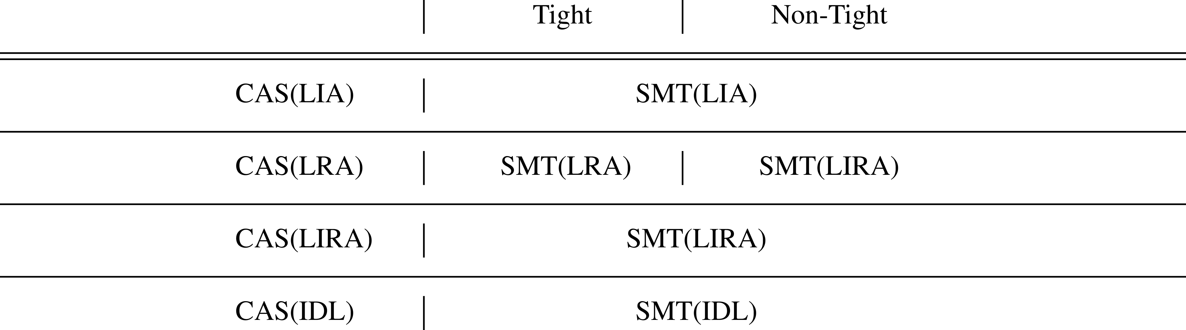
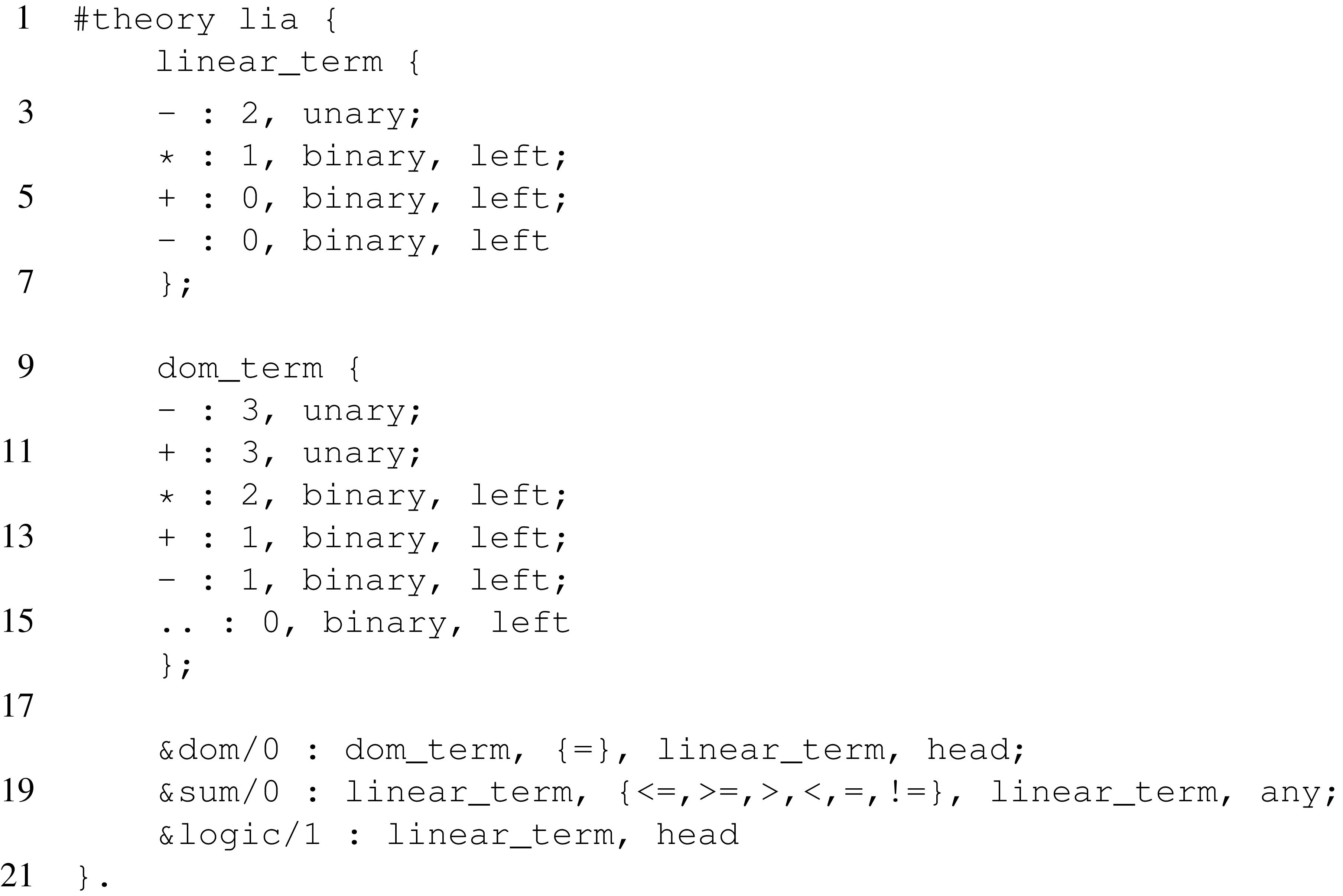
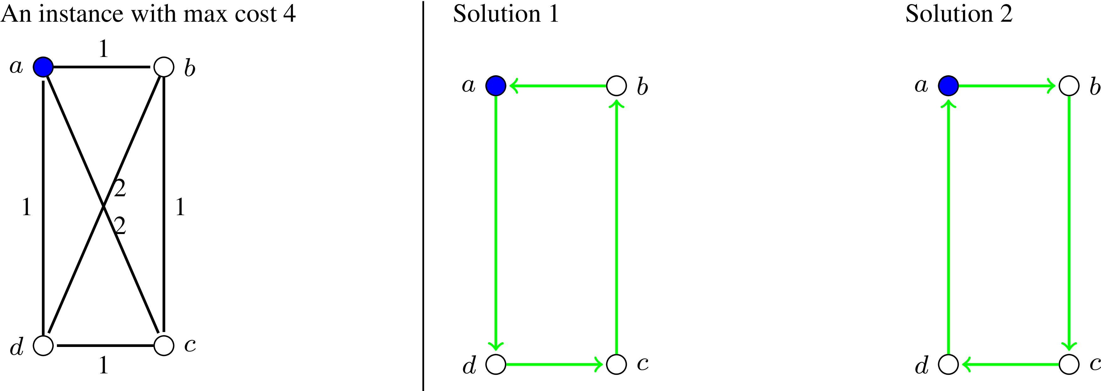
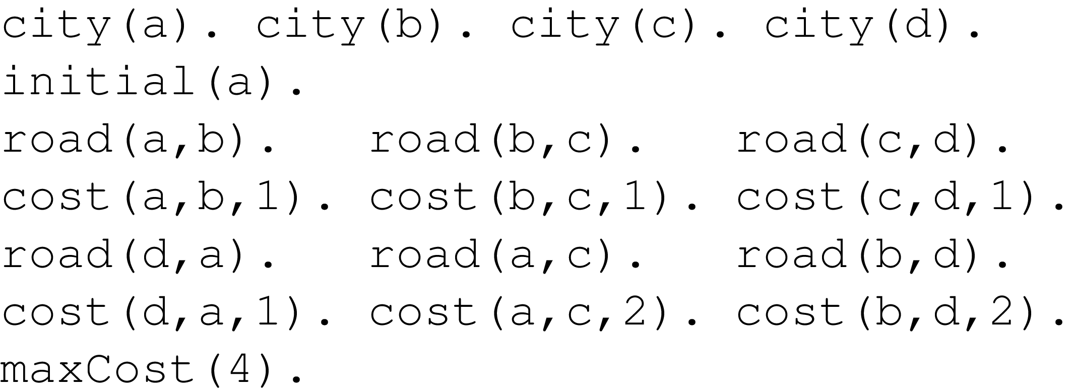
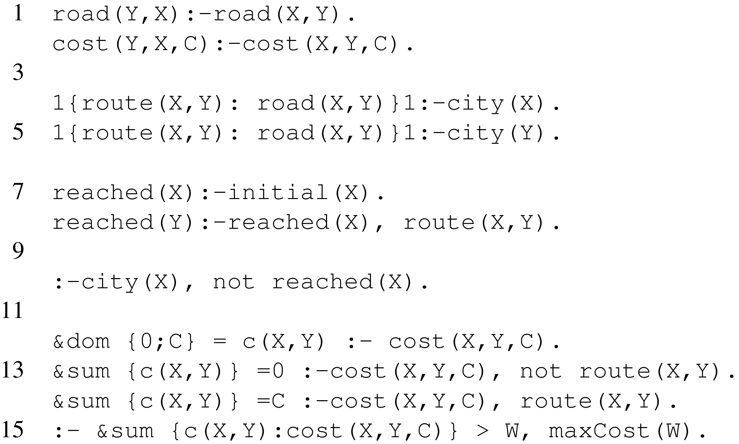

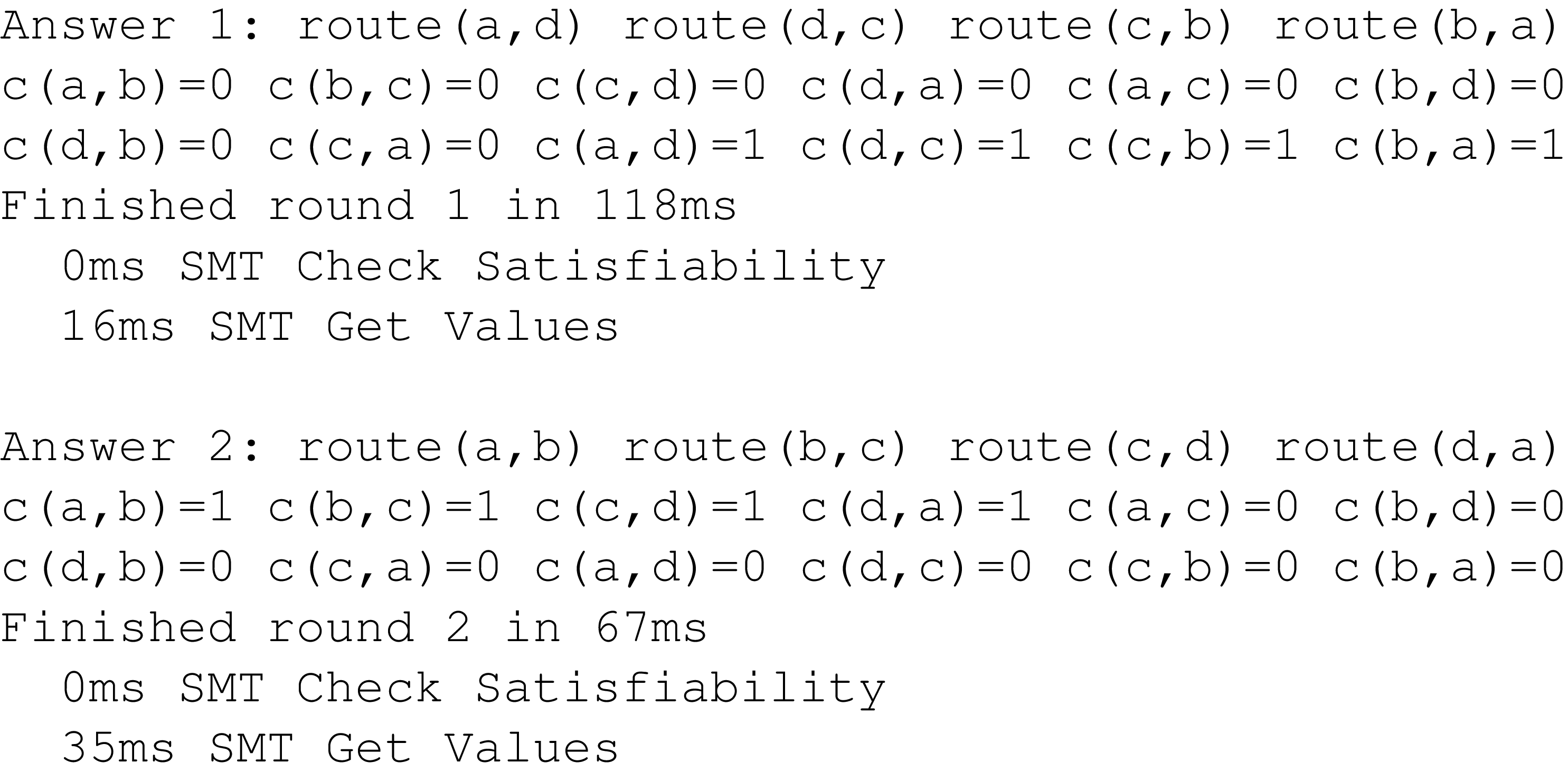
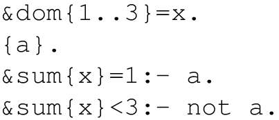
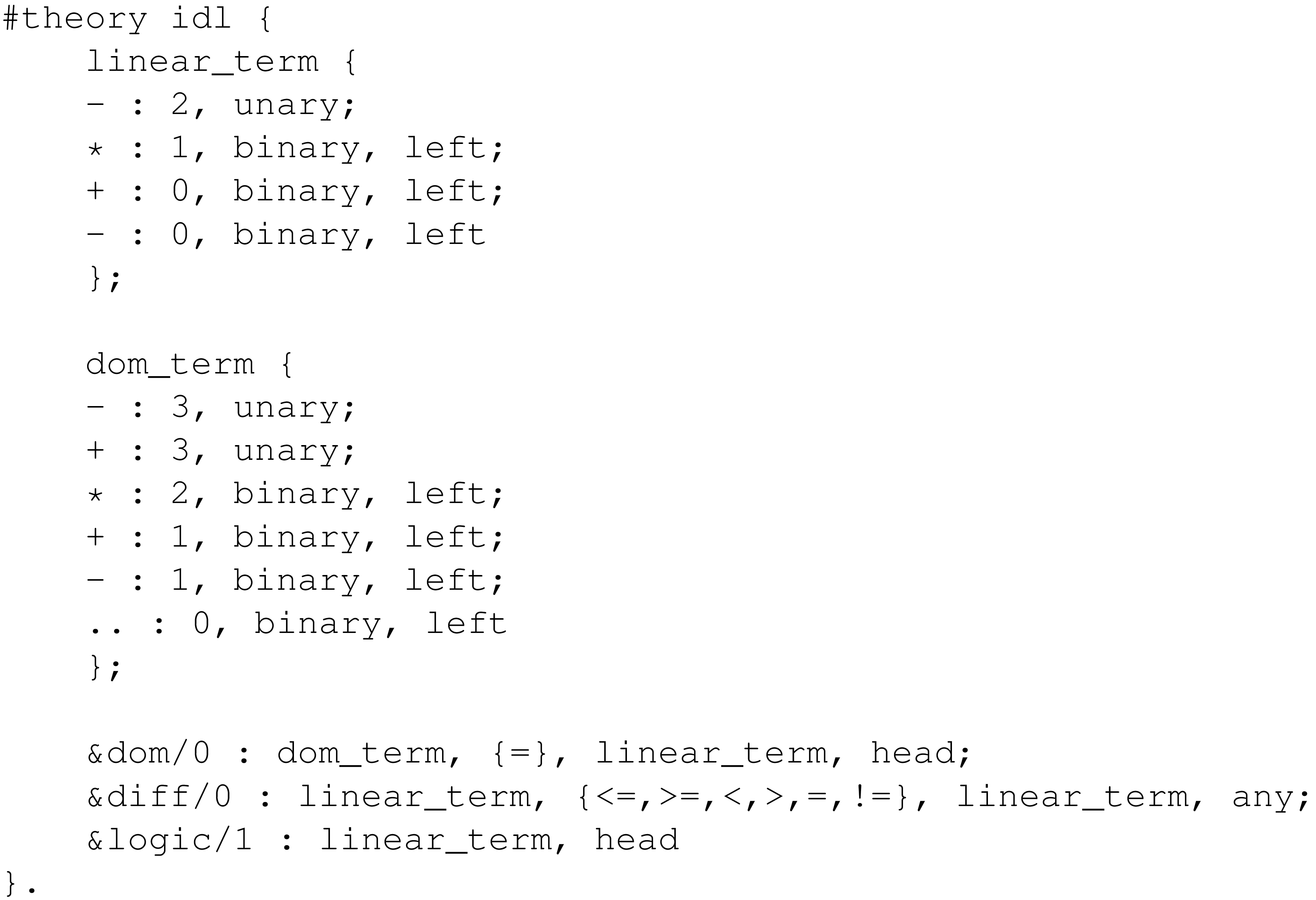

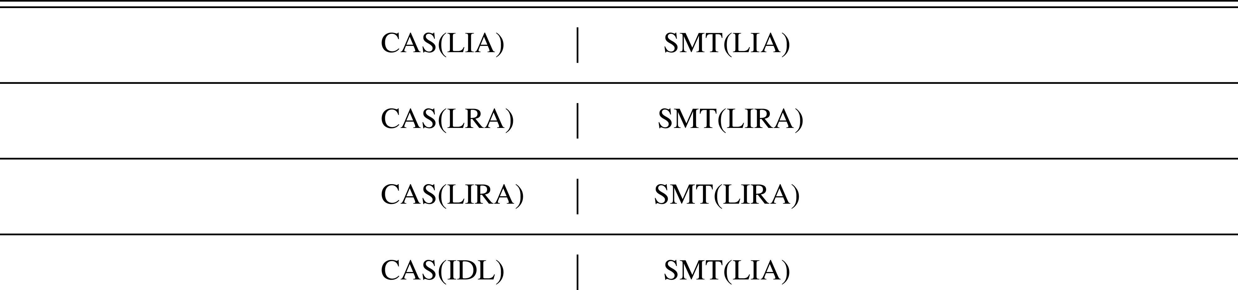


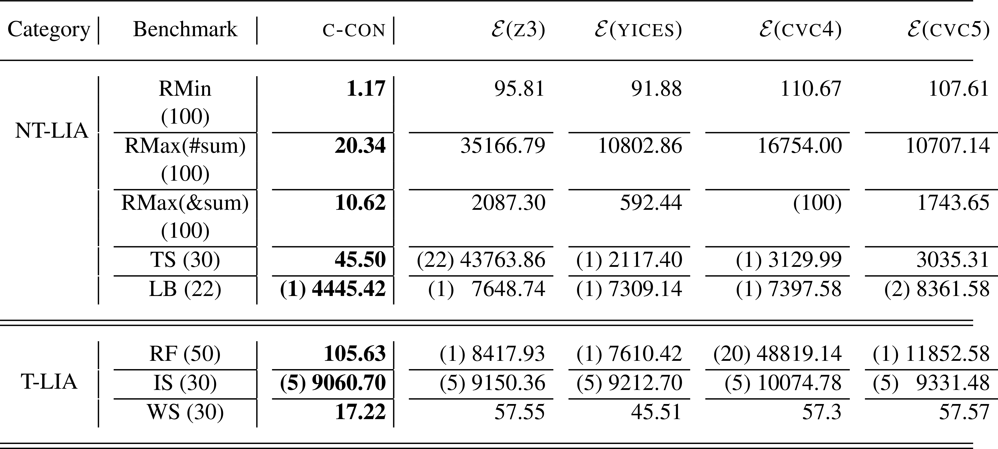
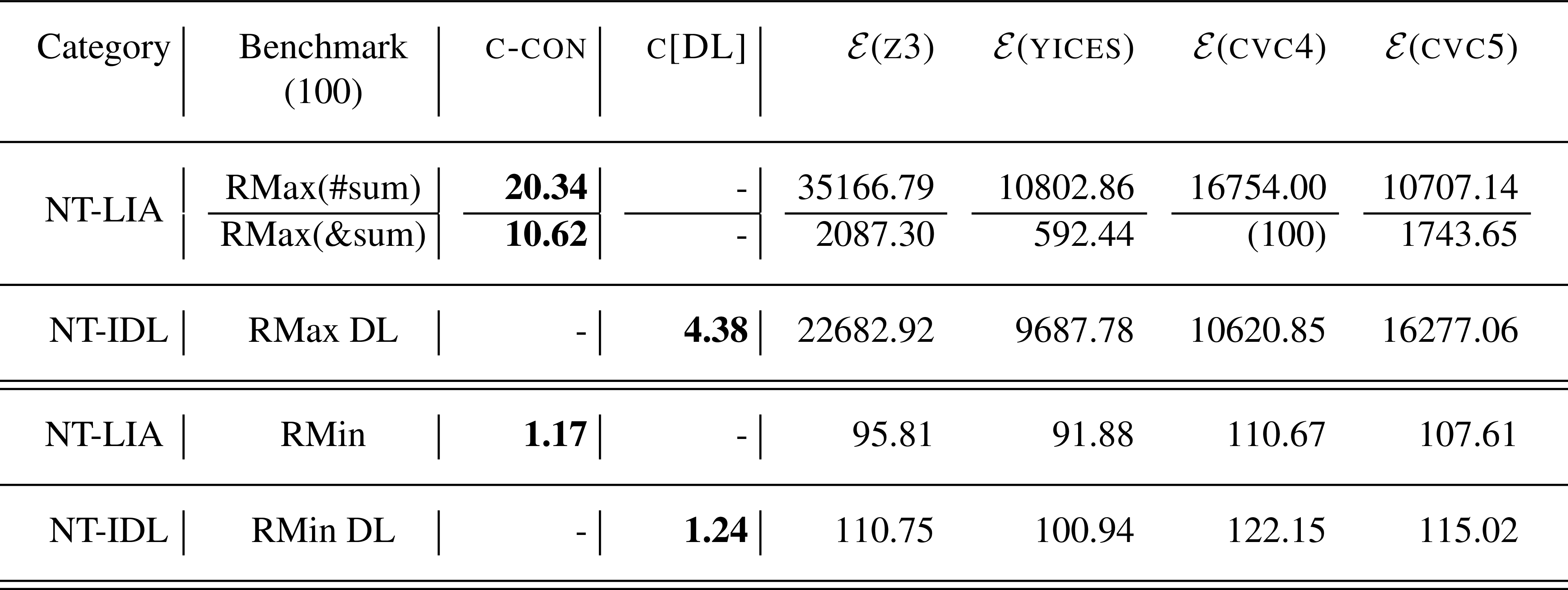

 Open access

