Introduction
Today, the planar patch antennas are used in different attractive modern wireless applications [Reference Garg, Bhartia, Bahl and Ittipiboon1–Reference Sung22]. So, the accurate determination of performance properties of the patch antenna is very essential. The resonant frequency fr for the patch antenna is the main design parameter because it determines the patch dimension, quality factors QT, input impedance Zin, directivity D, efficiency η, gain G, B.W, etc. Thus, the accurate determination of fr is very essential. The fr strongly varies with patch dimension, substrate thickness h, permittivity ɛr, and air gap h 2 between substrate and ground plane. So, the accurate prediction of fr as a function of above such variables is very essential. For the microstrip patch antenna, the fringing fields are at the edge so the analysis of planar patch antennas becomes critical. In order to determine the performance properties of patch antennas, the engineers require an easier design guideline to compute fr accurately.
The Zin of the coaxial probe should be matched with the Zin of the patch for radiating the maximum power. Thus, the Zin of a probe-fed planar patch antenna is another important design parameter. The Zin of the planar circular disc varies with the feed position ρ beneath the circular disc, disc radius r, fr, QT, and substrate electrical parameters. So, the accurate prediction of Zin in terms of above such variables is also necessary to install it properly into communication systems. Zin is calculated in terms of QT. The efficiency η is determined by the ratio of QT to the radiation loss Qr. The D and G are also depending on loss. The QT depends on r, fr, substrate electrical parameters, and air gap. Thus, the accurate determination of QT (loss) is also more essential to measure the performance properties of patch antennas.
The current passes through the central conductor of a coaxial probe produces an inductive reactance which is called the probe reactance XF. The input impedance between patch and probe does not match properly due to probe reactance. The probe reactance depends on ρ, probe diameter d, fr, and substrate electrical parameters. So, the accurate determination of probe reactance as the function of above such parameters is also very important.
In order to estimate the performance properties of microstrip patch antennas, several techniques have been reported. They are mainly two types: simple analytical methods [Reference Watkins23–Reference Antoszkiewicz and Shafai38] and rigorous numerical methods [Reference Yano and Ishimaru39–Reference Reineix and Jecko51]. The rigorous numerical methods such as Green's function technique [Reference Yano and Ishimaru39, Reference Aberle, Pozar and Birtcher40], mode matching technique [Reference Mehler, Maclean and Abbas41, Reference Davidovitz and Lo42], Galerkin method [Reference Davidovitz and Lo43, Reference Losada, Boix and Horno44], method of moment [Reference Newman and Tulyathan45–Reference Pozar and Voda48], spectral domain analysis [Reference Fan and Lee49], finite element method [Reference McGrath and Pyati50], and finite difference time domain method [Reference Reineix and Jecko51] provide more accurate results. However, rigorous numerical methods require precise mathematical formulations and it involves extensive numerical procedures. Also, they are computationally slow. So, the rigorous numerical methods are not well suited for determining the performance parameters of the patch antenna.
The simple analytical model such as cavity model [Reference Watkins23–Reference Antoszkiewicz and Shafai38] is one of the most extensively used methods for estimating the performance parameters of a circular microstrip patch antenna in comparison with rigorous numerical methods. The cavity model provides a physical perception which is normally absent in most of the numerical methods. Cavity model also provides the equivalent circuit for analysis which is not obtained from numerical methods. The implementation of cavity model is also easier.
The different applications of circular patch antenna have been reported in [Reference Navarro and Chang52–Reference Navarro, Fun and Chang55]. The circular disc is relatively smaller than the rectangular geometry [Reference Garg, Bhartia, Bahl and Ittipiboon1]. It is only one-dimensional parameter geometry. So, the analysis of circular disc is easier than the rectangular patch. The circular patch takes less area for array configurations. The fr, Zin, and radiation pattern values can be easily changed with the modification of circular disc.
The models available in the open literature [Reference Watkins23–Reference Antoszkiewicz and Shafai38] for computing the resonant frequency can give good results for the antenna parameters r/h > 2.0, ɛr < 10.0, and h/λg < 0.02, where λg is the wavelength in the substrate. Thus, the previously reported models [Reference Watkins23–Reference Antoszkiewicz and Shafai38] are not well valid for an antenna with small values of r/h and higher values of h/λg. For designing a millimeter-wave system, the electrically thick substrate (h/λg > 0.02) is required. The antennas fabricated for millimeter-wave system require high dielectric constant substrate. The antenna fabricated from high dielectric constant substrate behaves like an electrically thick substrate (h/λg > 0.02). The electrically thick substrate enhances the bandwidth. So, the analysis of a high permittivity substrate is also important for designing the electrically thick substrate antenna.
The fields at the edge of the circular disc are strongly modulated with the change of patch radius and substrate electrical parameters and that effect is computed in terms of effective dielectric constant ɛr,eff and effective patch radius reff [Reference Garg, Bhartia, Bahl and Ittipiboon1]. So, the accurate computation of these two parameters is needed for accurate estimation of the resonant frequency. But the models reported in [Reference Watkins23–Reference Antoszkiewicz and Shafai38] did not properly calculate ɛr,eff and reff for computing the resonant frequency. Thus, the models reported in [Reference Watkins23–Reference Antoszkiewicz and Shafai38] are inaccurate for computing the fr.
The cavity model reported in [Reference Richards, Lo and Harrison34–Reference Antoszkiewicz and Shafai38] for calculating the Zin in terms of r/h, electrical parameters of the substrate, and ρ is very erroneous. The models reported in [Reference Richards, Lo and Harrison34–Reference Antoszkiewicz and Shafai38] give good results for small values h/λg and ɛr. Also, previous models show a big error between measured and computed values with the variation of ρ.
Today, commercial software such as HFSS, CST, IE3D, CFDTD, etc., are also being employed to compute the performance parameters of patch antennas. But these software have some inherent limitations such as the software require the solution frequency and optimum probe position beneath the circular disc for computing the performance parameters of the antenna. The determination of this frequency and probe location is impossible without any mathematical model. Thus, the software need a number of trial and error processes for computing the important parameters of patch antennas which require additional time. So, the mathematical models based on simple expression and an equivalent circuit is essential for an antenna designer.
Considering all of these issues very carefully, we have targeted this problem in dual purposes: (i) we have proposed two comprehensive simple models to compute the fr, probe reactance XF, Zin, B.W, D, and G for a circular disc antenna. The models are developed by employing the cavity model and parallel resonant R-L-C circuit. These models are very simple and fast. The proposed models are capable of computing correctly the fr, QT, XF, and Zin for a large range of change of r/h, h/λg, and ɛr. The proposed models also accurately calculate the Zin with the variation of ρ over the entire radius, (ii) a large number of experiments are executed to verify the presented models.
Theory
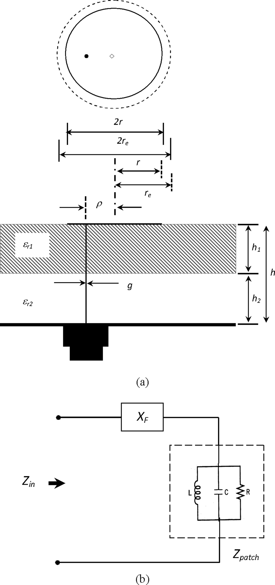
The Zin is the most important design parameter because it controls the efficiency and bandwidth. The impedance behavior of circular disc depicted in Fig. 1(b) is expressed in the form of parallel R-L-C circuit. The Zin with an inductive reactance is given by [Reference Biswas and Men56]:

where

(a) A schematic diagram of probe-fed circular microstrip patch antenna. (b) Equivalent resonant parallel R-L-C circuits.


where R is the resistance which is calculated in terms of resonant resistance Rr and field factor F(ρ), fr,mn is the mode-dependent resonant frequency, f is the working frequency, XP is the patch reactance, XF is the probe reactance, and m and n are the mode integers.
Probe reactance (XF)
For a coaxial probe fed patch antenna, the probe reactance XF and patch reactance XP are in series combination (Fig. 1(b)). The researcher [Reference Harrington57] proposed a very useful formula for determining the XF. Most of the researchers have employed the formula in [Reference Harrington57] for computing the probe reactance due to its simplicity. But this formula [Reference Harrington57] has some lacunae: (i) shows better results only near resonance; (ii) independent of probe location under the patch; and (iii) shows a large error with respect to experiments. The studies reported in [Reference Guha, Biswas and Siddiqui58, Reference Biswas and Dam59] show that the probe reactance highly depends on its location under the patch. To determine the XF in terms of ρ the research group [Reference Guha, Biswas and Siddiqui58, Reference Biswas and Dam59] multiplied the formula in [Reference Harrington57] by a complementary field factor. The modified formula reported in [Reference Guha, Biswas and Siddiqui58] is the function of both probe location and operating frequency but still there is a discrepancy. Here, we have employed the formula for probe reactance reported in [Reference Deshpande and Bailey60]. This formula [Reference Deshpande and Bailey60] is also independent of probe location under the patch. So, we have multiplied the formula in [Reference Deshpande and Bailey60] for probe reactance by a complementary field factor. This new formula is more accurate. Thus, the new probe reactance formula for a circular patch antenna in terms of f and ρ can be expressed as [Reference Biswas and Dam59]:

where F/(ρ) is the complementary field factor. XF (f) is the frequency-dependent probe reactance.
The XF (f) for rectangular geometry is computed from [Reference Deshpande and Bailey60] as

where


Here, η 0 is the intrinsic impedance = 377.7 ohm, d is the probe diameter, ɛre is the equivalent permittivity, and v0 is the free space light velocity. The expression (5) clearly shows that it is independent of ρ. We have employed the expression (5) to calculate XF (f) for circular geometry because it is independent of patch dimensions.
For computing the F(ρ) and F /(ρ) for a circular patch, we have employed two models.
Model-I:
For this model, F(ρ) is computed as

Thus, the F /(ρ) becomes

Model-II:
The F(ρ) for this model is obtained from

Thus, the F /(ρ) becomes

In expressions (6)–(9), αmn is the n th zero derivative of the Bessel function of order m, Jm is the Bessel function of order m, and re is the effective patch radius. Equation (4i) is the function of both probe location and frequency.
From equations (6) and (8), we can say that the F(ρ) is maximum at the edge (ρ = r) of the patch and decreases gradually if the probe moves toward the center from the edge and becomes minimum when the probe is located at the center (ρ = 0). This is based on the fact that the electric field is maximum at the edge of the patch and decreases gradually from the edge to the center of the patch and becomes minimum at the center. For this reason, the input impedance is maximum at the edge and then decreases gradually from the edge to the center and becomes minimum at the center. The simulation study shows that the probe reactance is maximum at the center and decreases gradually with the movement of the probe from the center to the edge and becomes minimum at the edge. Thus, the probe reactance follows the complementary profile of input impedance. So, a complementary field factor F/(ρ) is required to calculate the probe reactance as a function of ρ. The F/(ρ) defined in (7) and (9) has the complementary profile of F(ρ).
Total loss (QT)
The total loss QT consists of loss due to radiation (Qr), dielectric (Qd), and conductor (Qc). The total loss is computed as

Radiation loss (Qr)
For computing Qr, we have employed two models.
Model-I:
The loss due to radiation is obtained from [Reference Garg, Bhartia, Bahl and Ittipiboon1] as

where kr = αmn, k = kr,mn (ɛre)(1/2). I(X) = 1/D(X). D(X) is directivity. D(X) is obtained from curve fitting formula as

where


Model-II:
The Qr of a circular patch antenna is computed from the expression of Qr for a rectangular geometry. The simplest expression for computing the Qr of a rectangular patch antenna was reported in [Reference Bahl and Bhartia61] as

This relation is independent of modes and shows big discrepancy for thick substrate antenna. We have modified the relation (15i) for computing the Qr for a circular geometry as

here, ɛr,eff is the effective permittivity. The computed values employing the expressions (11) and (15ii) support well the experimental and simulation results for both electrically thick and thin substrate antenna. It is also mode-dependent.
Qd and Qc
Qd and Qc for both models are calculated as


Input resistance (R)
The input resistance may be defined as

here Rr is the resonant resistance. For computing Rr, we have employed two models.
Model-I:
The Rr for this model is obtained from originally formulated rectangular geometry of width a and length b [Reference Khellaf, Thouroude and Daniel62]. The Rr for a rectangular geometry is obtained as [Reference Khellaf, Thouroude and Daniel62]:

where ae is the effective patch width. For computing Rr for a circular patch antenna, we have employed an equivalent relation between rectangular and circular geometry of radius r. Here we have used an equivalent relation a = 1.142 r and b = 2 r [Reference Li and Bowler63]. Equation (20i) clearly shows that Rr is independent of modes. But Rr strongly depends on modes. So, we have modified equation (20i) for computing the mode-dependent Rr of a circular geometry as

here

where

From equations (20ii) and (20iii), we get the relation for Rr of a circular patch antenna as

Model-II:
We have previously stated that the models reported in [Reference Richards, Lo and Harrison34–Reference Antoszkiewicz and Shafai38] for computing the Rr of a circular patch show big discrepancy for electrically thick substrate. Among them, the model reported in [Reference Derneryd36] for computing the Rr is simpler. In this model, we have modified the model reported in [Reference Derneryd36] for computing the Rr. The relation for computing the Rr for circular geometry was reported in [Reference Derneryd36] as

This relation shows better results for electrically thin substrate but shows big discrepancy for thick substrate antenna. In this model, we have modified the relation (21i) as

The drawbacks of the previous models [Reference Richards, Lo and Harrison34–Reference Antoszkiewicz and Shafai38] are eliminated by using the expressions (20v) and (21ii). These expressions show very good agreement with experimental and simulation results for a large change of r/h, h/λg, and ɛr. Also, the presented models accurately compute the R with all the ρ over the entire radius.
Effective patch radius (re)
The effective patch radius is computed as [Reference Abboud, Damiano and Papiernik37]:

For computing p we have employed two models.
Model-I:
In this model, p for a circular geometry is obtained from originally formulated rectangular geometry of width a and length b [Reference Wheeler64]. The effective length be for rectangular geometry was reported in [Reference Wheeler64] as

where


And another relation for be is obtained from [Reference Li and Bowler63] as

From (23) and (24v) we get

Substituting aeq from (24i) into (24vi) we get

p for circular geometry is obtained from (25) by employing an equivalent relation a = 1.142 r and b = 2 r [Reference Li and Bowler63]. Thus, p for the circular geometry becomes

Model-II:
In this model, p is computed from [Reference Chew and Kong29] as:

Equivalent substrate relative permittivity (ɛre)
The ɛre of this two-layer structure (Fig. 1(a)) is determined as

here h 1 is the thickness of the substrate with relative permittivity ɛr 1 and h 2 is the thickness of the layer below the substrate with permittivity ɛr 2 and h = h1 + h2.
Effective permittivity (ɛr,eff)
For computing ɛr,eff, we have employed two models.
Model-I:
The ɛr,eff of this two-layer structure is computed for this model as [Reference Edwards and Steer65]:

where q is called filling fraction. We have calculated q for this model as

ɛr,dyn is the dynamic permittivity.
Model-II:
In this model, the ɛr,eff is obtained from [Reference Edwards and Steer65] as:

where G is a purely empirical term whose value is <1. We have employed a relation for computing the G as

The f0 and fp are defined as


The expressions for computing the ɛrf and Z of a rectangular geometry were reported in [Reference Bahl and Bhartia61] as


The expressions for ɛrf and Z of a circular disc of radius r are obtained from the expressions (32iv) and (32v) by using an equivalent relation a = 1.142 r and b = 2 r [Reference Li and Bowler63]. Thus, the expressions for ɛrf and Z of a circular disc become


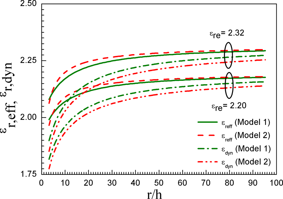
Here, we have calculated the effective permittivity ɛr,eff in term of ɛre and ɛr,dyn. The presented models give improved results. Most of the previously reported articles have considered either ɛre or ɛr,dyn for computing the fr. Figure 2 shows the importance of ɛr,eff. The variation of ɛr,eff and ɛr,dyn with the r/h for different ɛre is depicted in Fig. 2. This plot indicates that the ɛr,eff approaches to ɛr,dyn for a circular patch having large r/h values and varies remarkably for small r/h values. So, the term ɛr,eff incorporated in the presented models is applicable for a circular patch with a large variation of r/h.
Theoretical variation of ɛreff and ɛdyn as a function of r/h. h 1 = 1.575 mm, h 2 = 0.0 mm, h 1 = h, ɛr 2 = 1.0.

The lacunae of the previous models reported in [Reference Watkins23–Reference Antoszkiewicz and Shafai38] are eliminated by using the expressions (26), (27), (29), and (31).
The dynamic permittivity (ɛr,dyn)
The dynamic permittivity ɛr,dyn can be expressed as [Reference Wolff and Knoppik25]:

with

where Co,dyn is the dynamic main field capacitance without fringing field and Ce,dyn is the dynamic fringing field edge capacitance.
The Ce,dyn may be computed as


here Ce,stat(ɛ) represents the static fringing field capacitance. For computing Ce,stat, we have employed two models.
Model-I:
In this model, the Ce,stat for circular geometry is obtained from rectangular geometry. The Ce,stat for rectangular geometry is computed as [Reference Wolff and Knoppik25]:

where Co, stat (ɛ) is the static capacitance without fringing field and computed as

The Zr is computed from (32iii) with (33) and (34). The Ce,stat (ɛ) for a circular geometry is obtained from (39) by employing an equivalent relation a = 1.142 r and b = 2 r. Thus, Ce,stat (ɛ) for circular geometry becomes

with

Model-II:
For computing the static fringing field capacitance, we have employed the improved formula for the capacitance of a circular disk as reported in [Reference Wheeler66] as

where

(H) C 0,dyn (ɛ)
The C 0,dyn for circular patch is defined as

The Γm is in the form

Resonant frequency (fr,mn)
The mode-dependent resonant frequency using the cavity model analysis can be computed as

All the parameters in (47) are defined earlier.
The voltage standing wave ratio for <2.0 B.W can be obtained as

The gain (G) is defined as

For computing D, we have employed two models.
Model-I:
For model I, D is obtained from (12).
Model-II:
For this model, D is obtained from

Substrates for antenna fabrication and test
We have fabricated several prototypes from various PTFE materials such as: (i) Taconic having ɛr 1 = 2.33, h 1 = 0.7875, 1.5750 mm, tanδ 1 = 0.0012, (ii) Rogers with ɛr 1 = 2.40, h 1 = 0.8265, 1.580 mm, tanδ 1 = 0.0022, and (iii) Arlon with ɛr 1 = 9.80, h 1 = 1.630 mm, tanδ 1 = 0.0004. The coaxial feed of d = 1.270 mm was used to excite the patch. We have used Network Analyzer Agilent E5071B to perform several experiments.
Results and discussions
Resonant frequency fr
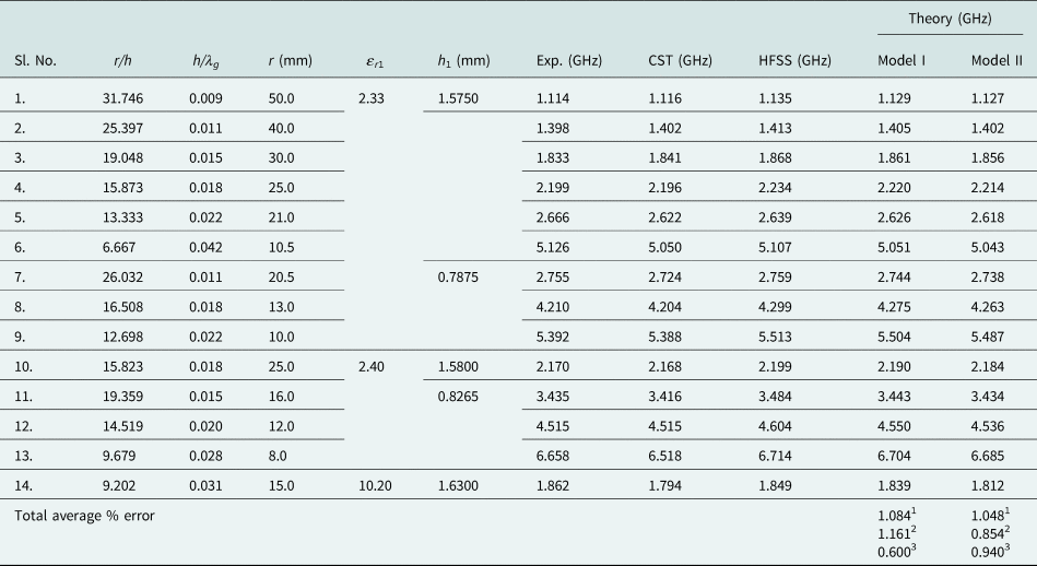
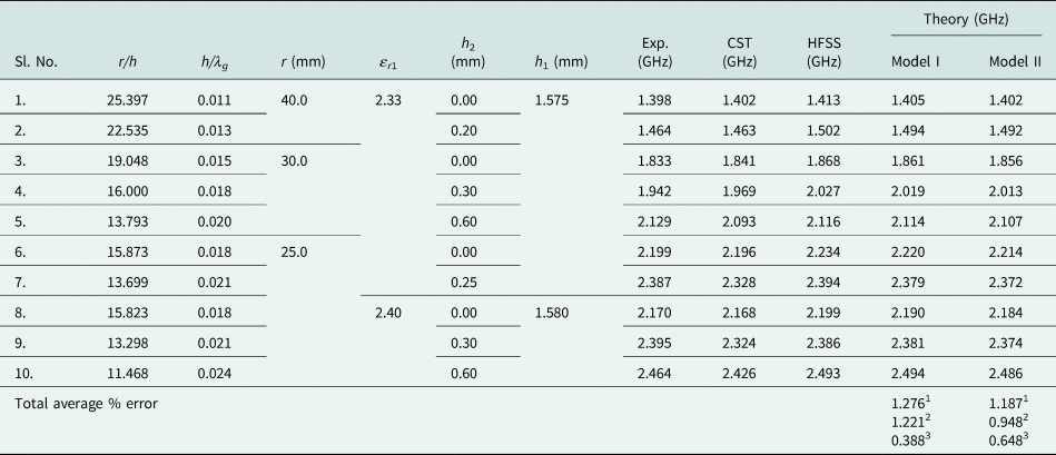
In Table 1, the theoretical fr employing the proposed models is compared with soft computing values (HFSS, CST) and our measured values for a circular patch etched on an electrically thick and thin substrate with varying r/h. The models accurately compute fr for a large variation of r/h and h/λg.
Comparison of theoretically predicted dominant mode resonant frequencies obtained from the present work for a circular microstrip patch with varying R/H, ɛR, H/λg with simulation (HFSS, CST) and our experimental results

h 2 = 0.0 mm, h = h 1, ɛr 2 = 1.0.
‘1’ w.r.t Expt., ‘2’ w.r.t. CST, ‘3’ w.r.t. HFSS.
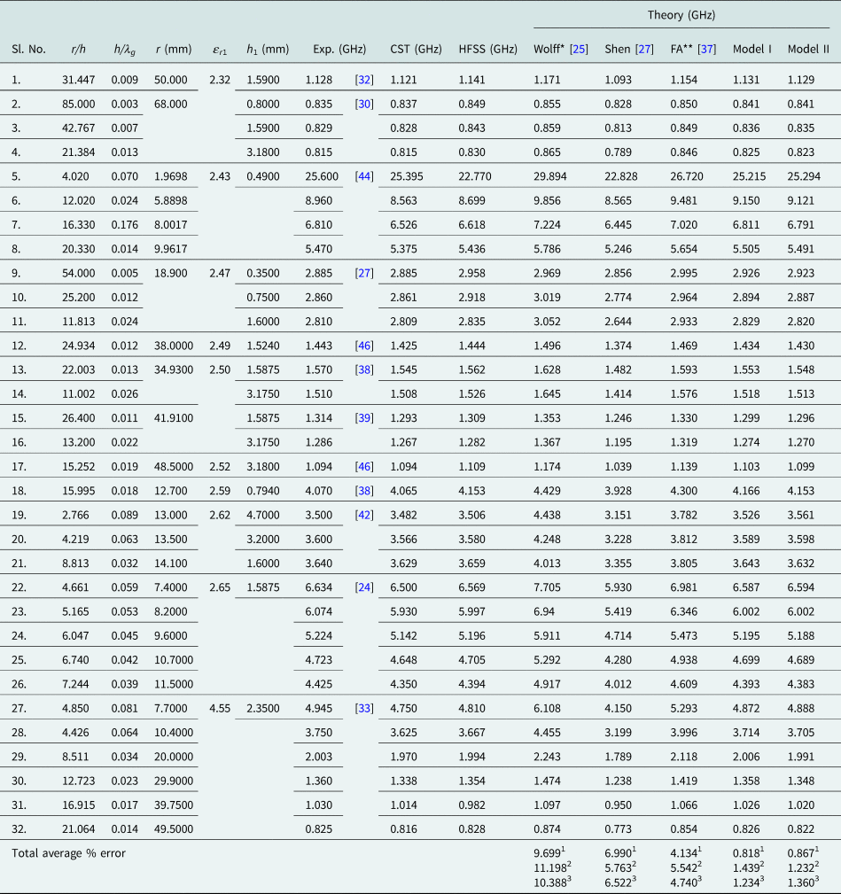
The accuracy of the presented models is further verified in Table 2. Here, we compare the computed fr using the presented models and the models reported in [Reference Wolff and Knoppik25, Reference Shen, Long, Allerding and Walton27, Reference Abboud, Damiano and Papiernik37] with the corresponding experimental [Reference Itoh and Mitra24, Reference Shen, Long, Allerding and Walton27, Reference Dahele and Lee30, Reference Dahele, Mem and Lee32, Reference Abboud, Damiano and Papiernik33, Reference Antoszkiewicz and Shafai38, Reference Yano and Ishimaru39, Reference Davidovitz and Lo42, Reference Losada, Boix and Horno44, Reference Carver and Mink46] and simulation (HFSS, CST) results for a circular patch fabricated from the electrically thick and thin substrate. The models reported in [Reference Wolff and Knoppik25, Reference Abboud, Damiano and Papiernik37] have been employed in the static fringing field capacitance Ce,stat = C 0,stat (1.0 + p). But this is the expression for total capacitance C following (43) of the previous section. Thus, Ce,stat is incorrectly evaluated in [Reference Wolff and Knoppik25, Reference Abboud, Damiano and Papiernik37]. For models [Reference Wolff and Knoppik25, Reference Abboud, Damiano and Papiernik37], we have correctly computed the Ce,stat following (44) of the theoretical section. The presented models are more accurate compared to the other models.
Comparison of experimental dominant mode resonant frequencies of circular microstrip patch with varying r/h, ɛr, h/λg from [Reference Itoh and Mitra24, Reference Shen, Long, Allerding and Walton27, Reference Dahele and Lee30, Reference Dahele, Mem and Lee32, Reference Abboud, Damiano and Papiernik33, Reference Antoszkiewicz and Shafai38, Reference Yano and Ishimaru39, Reference Davidovitz and Lo42, Reference Losada, Boix and Horno44, Reference Carver and Mink46] with simulation (HFSS, CST) and theoretically predicted values obtained from [Reference Wolff and Knoppik25, Reference Shen, Long, Allerding and Walton27, Reference Abboud, Damiano and Papiernik37] and in this work

h 2 = 0.0 mm, h = h 1, ɛr 2 = 1.0.
* and ** with correct expression of Ce,stat as in equation (43).
‘1’ w.r.t Expt., ‘2’ w.r.t. CST, ‘3’ w.r.t. HFSS.
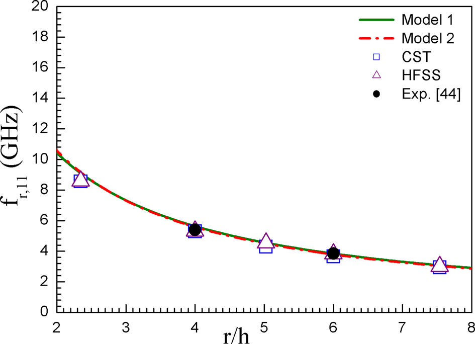
Figure 3 depicts a comparison of computed curves employing the presented models with experimental [Reference Losada, Boix and Horno44] and simulation (HFSS, CST) results for higher dielectric constant substrate (ɛr = 10.0) circular patch antenna. The models show excellent validation with measured and soft computing values. Thus, the models are suitable for designing higher dielectric constant circular patch antenna.
Theoretical, experimental [Reference Losada, Boix and Horno44], and simulation (HFSS, CST) variation of fr, 11 as a function of r/h. h 1 = 1.1938 mm, h 2 = 0.0 mm, h 1 = h, ɛr 1 = 10.0, ɛ r2 = 1.0.

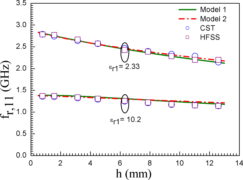
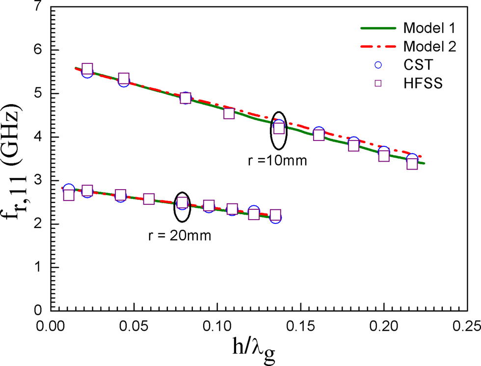
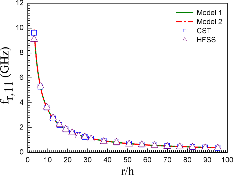
The effect of h on fr for different ɛr (ɛr = 2.33, 10.2) is visualized in Fig. 4. The computed fr employing the presented models are validated with soft computing (HFSS, CST) results. The theoretical and simulation (HFSS, CST) change of fr with the change of h/λg for two different antennas (r = 10, 20 mm) is shown in Fig. 5. The presented models accurately compute fr for a wide variation of h/λg (>0.22). The theoretical and simulation (HFSS, CST) variation of fr with r/h is depicted in Fig. 6. In this study, h is fixed but r is varying. The models accurately compute fr for a wide variation of r/h.
Theoretical and simulation (HFSS, CST) variation of fr, 11 as a function of h for two different values of ɛr. r = 20.0 mm, h 2 = 0.0 mm, h 1 = h, ɛr 2 = 1.0.

Theoretical and simulation (HFSS, CST) variation of fr, 11 as a function of h/λg for two different values of r. h 2 = 0.0 mm, h 1 = h, ɛr 1 = 2.33, ɛr 2 = 1.0.

Theoretical and simulation (HFSS, CST) variation of fr, 11 as a function of r/h. h 1 = 1.575 mm, h 2 = 0.0 mm, h 1 = h, ɛr 1 = 2.33, ɛr 2 = 1.0.

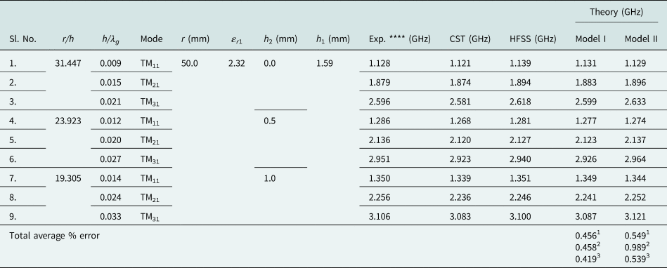
In Table 3, we have compared the computed fr with simulation (HFSS, CST) and our measured values for circular patches with air gap. Here, the air gap thickness is changing. The models support well to the measured and simulated values. The accuracy of the present models is further verified in Table 4. Here the computed fr for dominant and higher order modes employing the proposed models are verified with measured [Reference Dahele, Mem and Lee32] and simulated (HFSS, CST) values. The models show an error <1%.
Comparison of theoretically predicted dominant mode resonant frequencies obtained from our work for a circular microstrip patch with varying air gap, r/h, ɛr, h/λg with simulation (HFSS, CST) and our experimental results

ɛr 2 = 1.0, h = h 1+h 2.
‘1’ w.r.t Expt., ‘2’ w.r.t. CST, ‘3’ w.r.t. HFSS.
Comparison of theoretically predicted dominant and higher order modes of resonant frequencies employing present models for a circular microstrip patch with varying air gap, r/h, ɛr, h/λg with simulation (HFSS, CST) and experimental results [Reference Dahele, Mem and Lee32]

ɛr 2 = 1.0, h = h 1+h 2.
‘1’ w.r.t Expt., ‘2’ w.r.t. CST, ‘3’ w.r.t. HFSS.
From the above studies, we observe that the fr is changed with the change of patch radius, substrate electrical parameters, and air gap.
Probe reactance XF
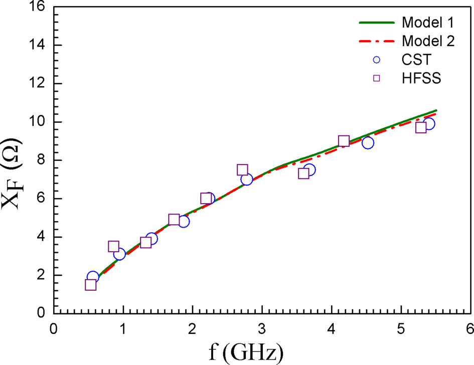
Figure 7 depicts the theoretical and simulation (HFSS, CST) variations of XF with the variation of f. The XF increases with the increase of f. The theoretical curves support very well to the simulation values.
Theoretical and simulation (HFSS, CST) variation of XF as a function of f. h 1 = 0.7875 mm, h 2 = 0.0 mm, h 1 = h, ɛr 1 = 2.33, ɛr 2 = 1.0, d = 1.27 mm.

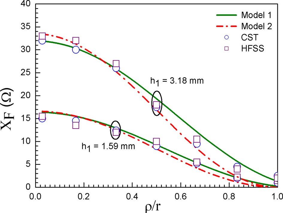
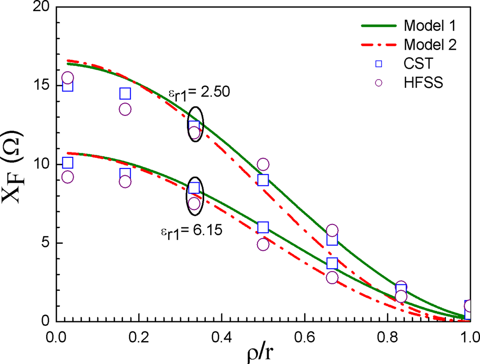
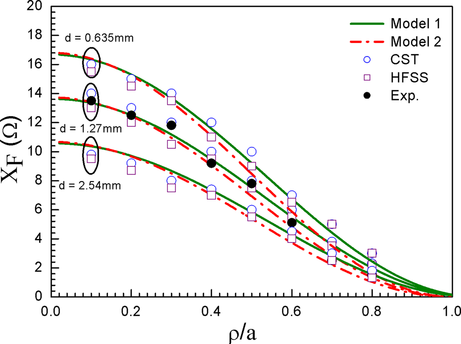
The variation of XF with the variation of ρ/r for different values of h and ɛr is depicted in Figs 8 and 9. The theoretical curves are compared with simulation (HFSS, CST) results. The presented models show closer agreements with simulation results for all values of ρ/r, h, and ɛr. In Fig. 10, we have verified our models with simulation (HFSS, CST) and our experimental results for different probe diameter d. The models accurately calculate the XF for all ρ/r and d. Thus, the XF depends on both frequency and probe location. We have also examined that the XF is changed significantly with the change of substrate electrical parameters and probe diameter.
Theoretical and simulation (HFSS, CST) variation of XF as a function of ρ/r for different values of h. r = 18.0 mm, h 2 = 0.0 mm, h 1 = h, ɛr 1 = 2.50, ɛr 2 = 1.0, d = 1.27 mm.

Theoretical and simulation (HFSS, CST) variation of XF as a function of ρ/r for different values of ɛr. r = 18.0 mm, h 1 = 1.59 mm, h 2 = 0.0 mm, h 1 = h, ɛr 2 = 1.0, d = 1.27 mm.

Theoretical, new experimental, and simulation (HFSS, CST) variation of XF as a function of ρ/r for different d. r = 25.0 mm, h 1 = 1.575 mm, h 2 = 0.0 mm, h 1 = h, ɛr 1 = 2.33, ɛr 2 = 1.0, tanδ 1 = 0.0012, tanδ 2 = 0.000, g is variable.

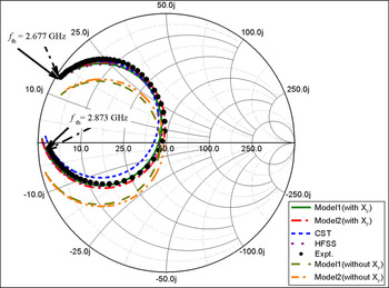
The effect of XF on impedance characteristic is shown in Fig. 11. Here, the theoretical input impedances with and without probe reactance employing the presented models are compared with simulation (HFSS, CST) and our experimental results. A discrepancy between theoretical and experimental results is observed when XF is not included with the input impedance but excellent agreement reveals between theoretical and experimental results when XF is included with the input impedance. This study indicates the necessity of probe reactance.
Theoretical, new experimental, and simulation (HFSS, CST) variation of input impedance with f. r = 20.5 mm, h 1 = 0.7875 mm, h 2 = 0.0 mm, h 1 = h, ɛr 1 = 2.33, ɛr 2 = 1.0, frav,m 1 = 2.744 GHz, frav,m 2 = 2.738 GHz, fmea = 2.755 GHz, tanδ 1 = 0.0012, ρ = 5.0 mm, h/λ g = 0.011, frequency increment = 0.001 GHz, d = 1.27 mm.

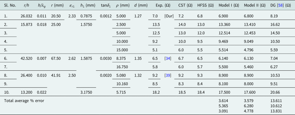
We have previously stated that the proposed models are more accurate than the previous model [Reference Guha, Biswas and Siddiqui58]. This is further verified in Table 5. The theoretical XF using our models and models reported in [Reference Guha, Biswas and Siddiqui58] are compared with our measured values and measured values reported in [Reference Richards, Lo and Harrison34, Reference Yano and Ishimaru39]. The presented models show about 3.5% error whereas the previous model [Reference Guha, Biswas and Siddiqui58] shows about 13.5% error against the experimental results.
Comparison of experimental probe reactance XF of circular microstrip patch with varying r/h, ɛr, h/λg, ρ, d from [Reference Richards, Lo and Harrison34, Reference Yano and Ishimaru39] and with simulation (HFSS, CST) and predicted values obtained from [Reference Guha, Biswas and Siddiqui58] and in this work

h 2 = 0.0 mm, h = h 1, ɛr 2 = 1.0.
‘1’ w.r.t Expt., ‘2’ w.r.t. CST, ‘3’ w.r.t. HFSS.
From the above studies, we observe that the probe reactance is changed with the frequency, probe location, probe diameter, and electrical parameters of the substrate. Thus, the accurate computation of probe reactance is very essential for proper impedance matching between probe and patch.
Q T, B.W, and G
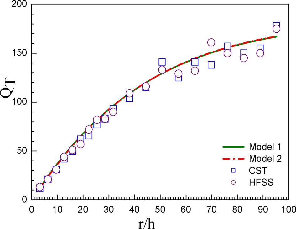
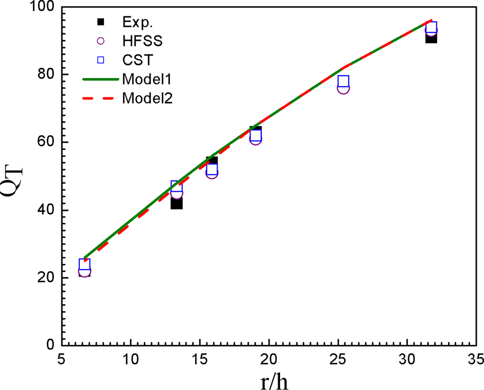
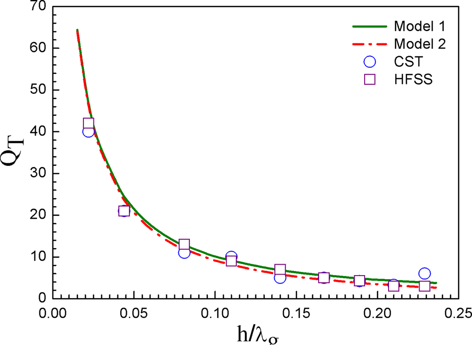
In Fig. 12, the change of theoretical and simulation (HFSS, CST) values of QT with the change of r/h is visualized. Here, we consider that r is varying and h is a fixed value. QT increases with the increase of r/h. The presented models accurately calculate the QT for any values of r/h. The validation of presented models is further verified in Fig. 13. Here, we have compared computed values employing the presented model with simulation (HFSS, CST) and our experimental results. The close correlation is achieved between the computed curves, simulation, and experimental results. In Fig. 14, authors present the theoretical and simulation (HFSS, CST) variations of QT with h/λg. The models show closer agreements with soft computing results for a large change of h/λg up to 0.22.
Theoretical and simulation (HFSS, CST) variation of QT with r/h. h 1 = 1.575 mm, h 2 = 0.0 mm, h 1 = h, ɛr 1 = 2.33, ɛr 2 = 1.0, tanδ 1 = 0.0012, tanδ 2 = 0.000.

Theoretical, new experimental, and simulation (HFSS, CST) variation of QT with r/h. h 1 = 1.575 mm, h 2 = 0.0 mm, h 1 = h, ɛr 1 = 2.33, ɛr 2 = 1.0, tanδ 1 = 0.0012, tanδ 2 = 0.000.

Theoretical and simulation (HFSS, CST) variation of QT with h/λg; r = 10.0 mm, h 2 = 0.0 mm, h 1 = h, ɛr 1 = 2.33, ɛr 2 = 1.0, tanδ 1 = 0.0012, tanδ 2 = 0.000.

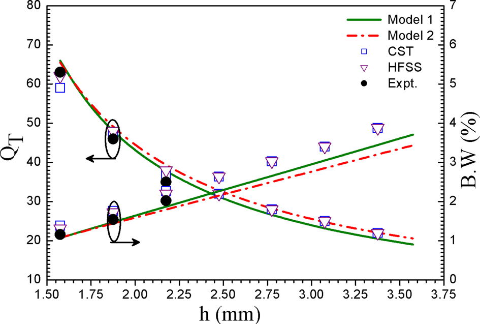
The variation of total loss and %B.W with the change of h for a circular patch is depicted in Fig. 15. Here the substrate thickness h 1 is fixed but h 2 is varied. The theoretical curves support well to the simulation (HFSS, CST) and our experimental results. The bandwidth is enhanced due to the introduction of air gap without change of any antenna parameters.
Theoretical, new experimental, and simulation (HFSS, CST) variation of QT and bandwidth with h. r = 30.0 mm, h 1 = 1.575 mm, h 2 variable, ɛr 1 = 2.33, ɛr 2 = 1.0, tanδ 1 = 0.0012, tanδ 2 = 0.000.

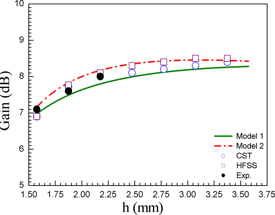
The change of gain with the change of h is depicted in Fig. 16. Here the substrate thickness h 1 is fixed but the air gap thickness h 2 is variable. The gain changes with the change of h 2. Thus, gain tunability is achieved. Here the computed curves are compared with our measured and simulated (HFSS, CST) values. The comparison shows that the present models support well to the simulated and measured gain. Thus, the quality factor determines the bandwidth and gain. The quality factor depends on patch radius, frequency, substrate electrical parameters, and air gap.
Theoretical, new experimental, and simulation (HFSS, CST) variation of gain with h. r = 25.0 mm, h 1 = 1.575 mm, h 2 variable, ɛr 1 = 2.33, ɛr 2 = 1.0.

Input impedance
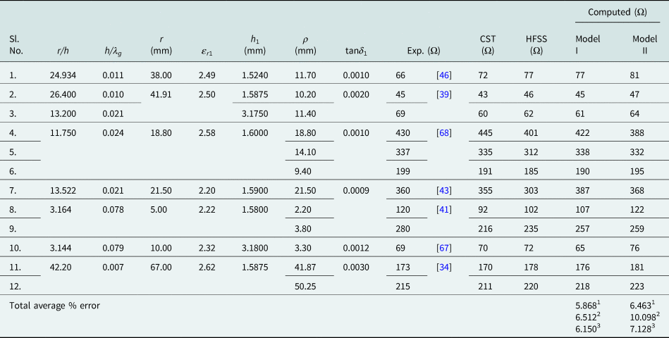
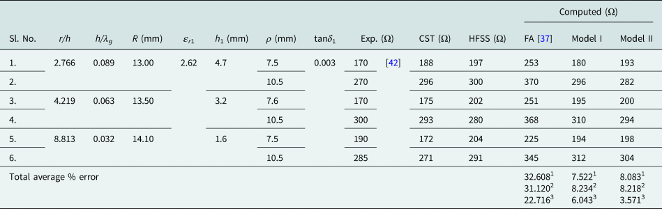
In Table 6, the authors compare computed R using the proposed models with the new experimental results and simulation results (HFSS, CST). The models show good accuracy against the measured and simulated values. The accuracy of the presented models is further verified in Table 7. Here, the computed values using the presented models are compared with the experimental values [Reference Richards, Lo and Harrison34, Reference Yano and Ishimaru39, Reference Mehler, Maclean and Abbas41, Reference Davidovitz and Lo43, Reference Carver and Mink46, Reference Bhattacharyya67, Reference Walton68] and simulation results (HFSS, CST). The presented models support well to the measured and simulated values. We have previously stated that the previous closed-form model [Reference Abboud, Damiano and Papiernik37] is not valid for electrically thick substrate antenna. This is verified in Table 8. The presented models show about 8% error, whereas the model in [Reference Abboud, Damiano and Papiernik37] shows about 33% error. Thus, the model reported in [Reference Abboud, Damiano and Papiernik37] shows big discrepancy for electrically thick substrate antenna.
Comparison of our experimental dominant mode input resistance of circular microstrip patch with varying r/h, ɛr, h/λg with simulation (HFSS, CST) and theoretically predicted values obtained from the present work

ɛr 2 = 1.0, h 2 = 0.0 mm.
‘1’ w.r.t Expt., ‘2’ w.r.t. CST, ‘3’ w.r.t. HFSS.
Comparison of experimental dominant mode input resistance of circular microstrip patch with varying r/h, ɛr, h/λg from [Reference Richards, Lo and Harrison34, Reference Yano and Ishimaru39, Reference Mehler, Maclean and Abbas41, Reference Davidovitz and Lo43, Reference Carver and Mink46, Reference Wheeler66, Reference Bhattacharyya67] with simulation (HFSS, CST) and theoretically predicted values obtained from the present work

ɛ r2 = 1.0, h 2 = 0.0 mm.
‘1’ w.r.t Expt., ‘2’ w.r.t. CST, ‘3’ w.r.t. HFSS.
Comparison of experimental dominant mode input resistance of circular microstrip patch with varying r/h, ɛr, h/λg from [Reference Davidovitz and Lo42] with simulation (HFSS, CST) and theoretically predicted values obtained from [Reference Abboud, Damiano and Papiernik37] and in this work for electrically thick substrate

ɛr 2 = 1.0, h 2 = 0.0 mm.
‘1’ w.r.t Expt., ‘2’ w.r.t. CST, ‘3’ w.r.t. HFSS.
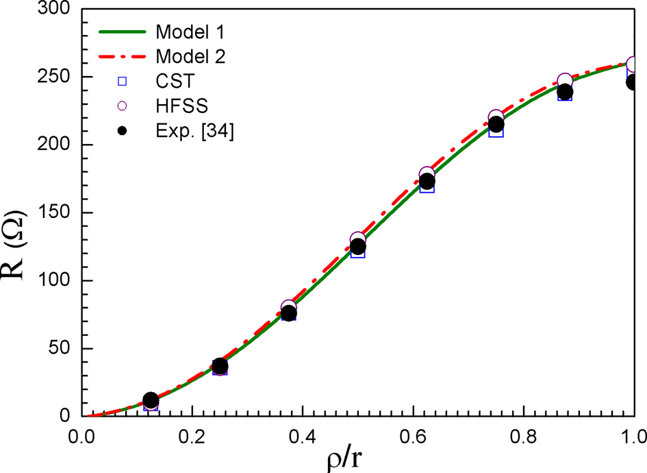
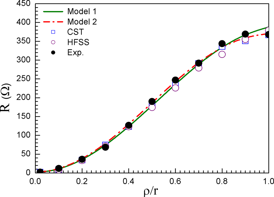
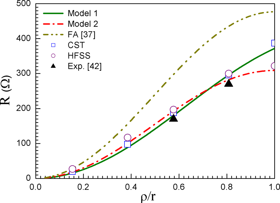
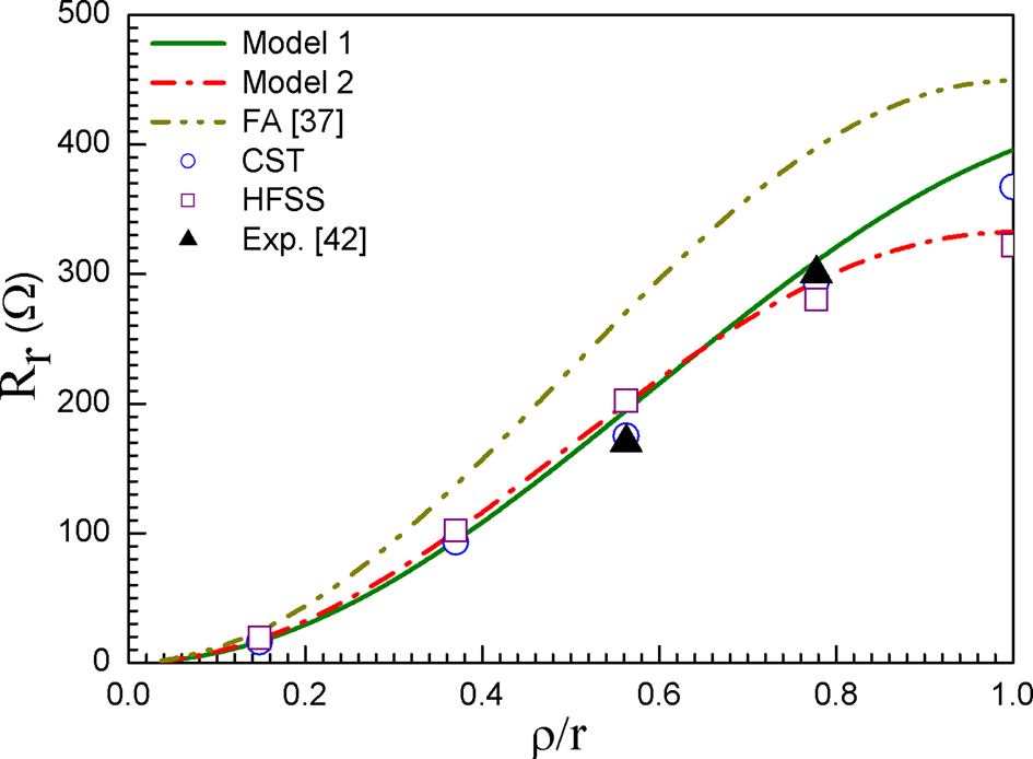
Figure 17 shows that the experimental [Reference Richards, Lo and Harrison34], simulation (HFSS, CST), and theoretical variations of R as a function of ρ/r. The presented models are again validated with new measured values depicted in Fig. 18. The models show excellent agreements with our measured values and measured values reported in [Reference Richards, Lo and Harrison34] and also support well the simulation results. The variation of R with the variation of ρ/r for electrically thick substrate antenna is shown in Figs 19 and 20. Here theoretically predicted results obtained with the presented models and the model reported in [Reference Abboud, Damiano and Papiernik37] are compared with the measured [Reference Davidovitz and Lo42] and simulated results (HFSS, CST). The proposed models show very good consistency with the measured and simulated values. But the model in [Reference Abboud, Damiano and Papiernik37] shows a big discrepancy.
Theoretical, simulation (HFSS, CST), and experimental [Reference Richards, Lo and Harrison34] variation of Rr as a function of ρ. r = 67.0 mm, h 1 = 1.5875 mm, h 2 = 0.0 mm, h 1 = h, ɛr 1 = 2.62, ɛr 2 = 1.0, tanδ 1 = 0.003, tanδ 2 = 0.000, h/λg = 0.007, d = 1.27 mm.

Theoretical, new experimental, and simulation (HFSS, CST) variation of Rr as a function of ρ. r = 25.0 mm, h 1 = 1.575 mm, h 2 = 0.0 mm, h 1 = h, ɛr 1 = 2.33, ɛr 2 = 1.0, tanδ 1 = 0.0012, tanδ 2 = 0.000, h/λg = 0.018, d = 1.27 mm.

Theoretical [present, 37], simulation (HFSS, CST), and experimental [Reference Davidovitz and Lo42] variation of Rr as a function of ρ. r = 13.0 mm, h 1 = 4.7 mm, h 2 = 0.0 mm, h 1 = h, ɛr 1 = 2.62, ɛr 2 = 1.0, tanδ 1 = 0.003, tanδ 2 = 0.000, h/λg = 0.089, d = 1.27 mm.

Theoretical [present, 37], simulation (HFSS, CST), and experimental [Reference Davidovitz and Lo42] variation of Rr as a function of ρ. r = 13.5 mm, h 1 = 3.2 mm, h 2 = 0.0 mm, h 1 = h, ɛr 1 = 2.62, ɛr 2 = 1.0, tanδ 1 = 0.003, tanδ 2 = 0.000, h/λg = 0.063, d = 1.27 mm.

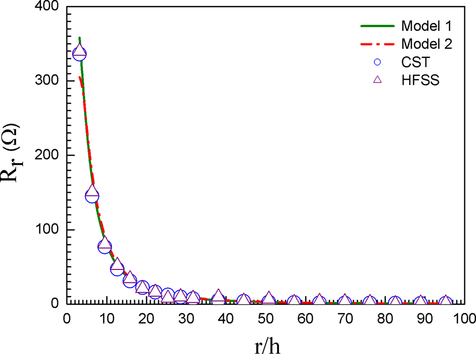
The theoretically computed and soft computed change of R with the variation of r/h is depicted in Fig. 21. The R decreases with the increase of r/h. A very close agreement is observed between simulation and computed curves for all r/h.
Theoretical and simulation (HFSS, CST) variation of Rr as a function of r/h. h 1 = 1.575 mm, h 2 = 0.0 mm, h 1 = h, ɛr 1 = 2.33, ɛr 2 = 1.0, tanδ 1 = 0.0012, tanδ 2 = 0.000, d = 1.27 mm.

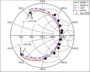
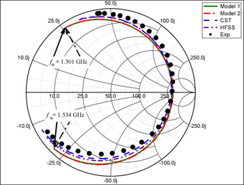
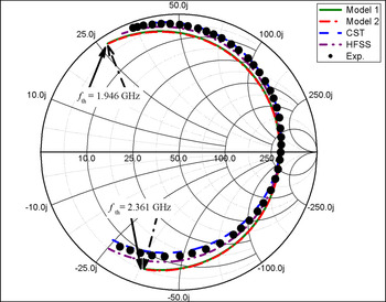
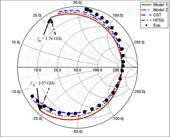
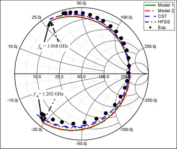
Figure 22 shows a comparison of measured [Reference Dahele, Mem and Lee32] and simulated (HFSS, CST) input impedance with the computed curves employing the presented models. The models show very close agreements with the measured and simulated values. The models are further verified in Figs 23–26 for a circular patch having the variable h/λg. The theoretical curves using the presented models are compared with simulation (HFSS, CST) and our experimental results. The models accurately calculate input impedance.
Theoretical, experimental [Reference Dahele, Mem and Lee32], and simulation (HFSS, CST) variation of input impedance with f. r = 50 mm, h 1 = 1.59 mm, h 2 = 0.0 mm, ɛr 1 = 2.32, ɛr 2 = 1.0, frav,m 1 = 1.131 GHz, frav,m 2 = 1.129 GHz, fCST = 1.121 GHz, fHFSS = 1.141 GHz, fmea = 1.128 GHz, tanδ 1 = 0.001, tanδ 2 = 0.000, ρ = 47.5 mm, d = 1.27 mm, h/λg = 0.009. Frequency increment = 0.001 GHz.

Theoretical, new experimental, and simulation (HFSS, CST) variation of input impedance with f. r = 40.0 mm, h 1 = 1.575 mm, h 2 = 0.0 mm, ɛr 1 = 2.33, ɛr 2 = 1.0, frav,m 1 = 1.405 GHz, frav,m 2 = 1.402 GHz, fCST = 1.402 GHz, fHFSS = 1.413 GHz, fmea = 1.398 GHz, tanδ 1 = 0.0012, tanδ 2 = 0.000, ρ = 32.0 mm, h/λg = 0.011, d = 1.27 mm. Frequency increment = 0.001 GHz.

Theoretical, new experimental, and simulation (HFSS, CST) variation of input impedance with f. r = 25 mm, h 1 = 1.58 mm, h 2 = 0.0 mm, ɛr 1 = 2.4, ɛr 2 = 1.0, frav,m 1 = 2.190 GHz, frav,m 2 = 2.184 GHz, fCST = 2.168 GHz, fHFSS = 2.184 GHz, fmea = 2.170 GHz, tanδ 1 = 0.0022, tanδ 2 = 0.000, ρ = 20.0 mm, h/λg = 0.018, d = 1.27 mm. Frequency increment = 0.001 GHz.

Theoretical, new experimental, and simulation (HFSS, CST) variation of input impedance with f. r = 30.0 mm, h 1 = 1.575 mm, h 2 = 0.0 mm, ɛr 1 = 2.33, ɛr 2 = 1.0, frav,m 1 = 1.861 GHz, frav,m 2 = 1.865 GHz, fCST = 1.841 GHz, fHFSS = 1.868 GHz, fmea = 1.833 GHz, tanδ 1 = 0.0012, tanδ 2 = 0.000, ρ = 24.0 mm, h/λg = 0.015, d = 1.27 mm. Frequency increment = 0.001 GHz.

Theoretical, new experimental, and simulation (HFSS, CST) variation of input impedance with f. r = 50.0 mm, h 1 = 1.575 mm, h 2 = 0.0 mm, ɛr 1 = 2.33, ɛr 2 = 1.0, frav,m 1 = 1.129 GHz, frav,m 2 = 1.127 GHz, fCST = 1.116 GHz, fHFSS = 1.135 GHz, fmea = 1.114 GHz, tanδ 1 = 0.0012, tanδ 2 = 0.000, ρ = 40.0 mm, h/λg = 0.009, d = 1.27 mm. Frequency increment = 0.001 GHz.

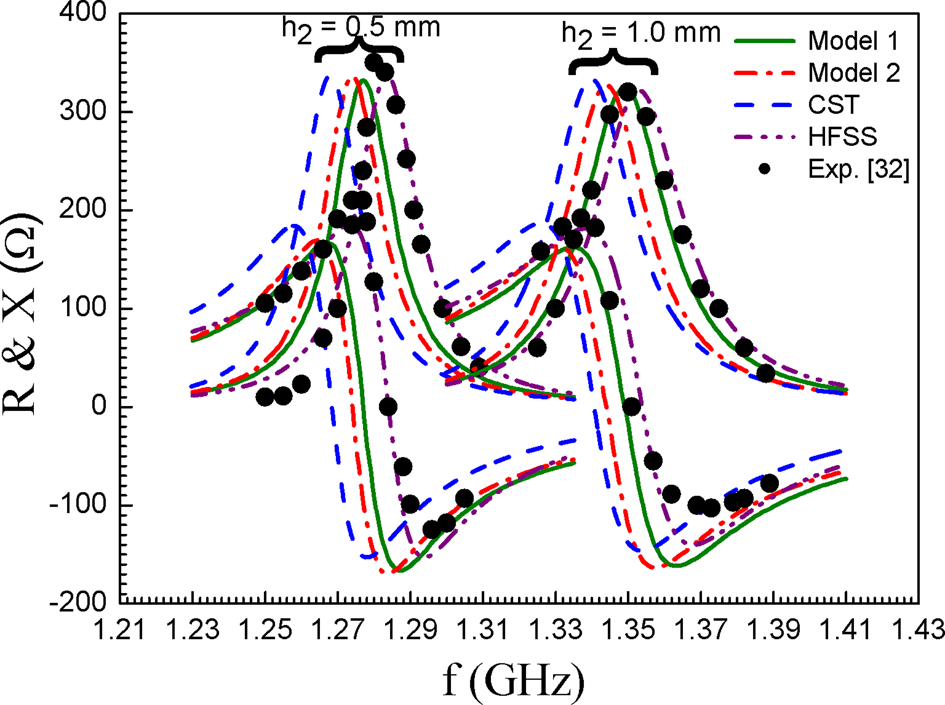
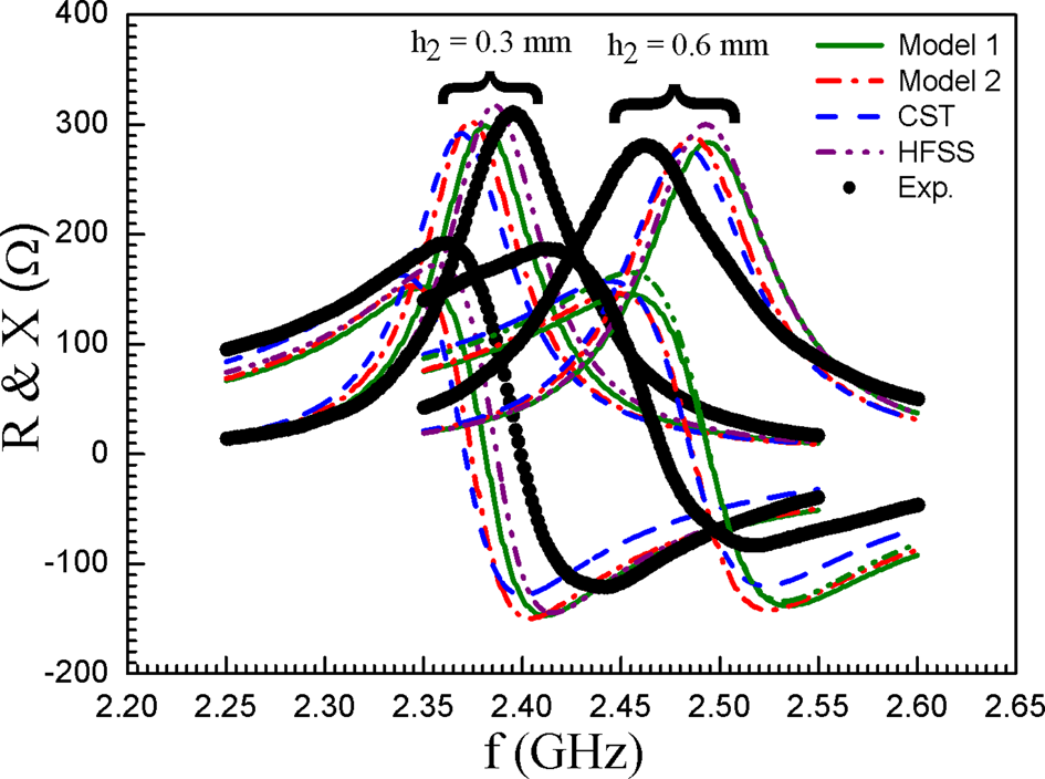
In Fig. 27, authors compare the theoretical curves employing the presented models with simulation (HFSS, CST) and experimental curves [Reference Dahele, Mem and Lee32] for two different air gap thicknesses h 2. The models are further verified with our new experimental results for two different h 2 depicted in Fig. 28. The models show very close agreements with the new measured results and measured results reported in [Reference Dahele, Mem and Lee32]. The presented models also validate well to the simulation results. From this plot, we see that the introduction of air gap causes the shift of fr to the upward. Thus, the frequency tunability is achieved with this structure. We also observe that the bandwidth is enhanced due to the introduction of air gap.
Theoretical, simulation (HFSS, CST), and experimental [Reference Dahele, Mem and Lee32] variation of resistance and reactance as a function of frequency f. r = 50.0 mm, h 1 = 1.59 mm, h 2 variable, ɛr 1 = 2.32, ɛr 2 = 1.0, tanδ 1 = 0.001, tanδ 2 = 0.000, ρ = 47.5 mm, h/λg = 0.012 (0.5 mm); h/λg = 0.014 (1.0 mm), d = 1.27 mm.

Theoretical, new experimental, and simulation (HFSS, CST) variation of resistance and reactance as a function of frequency. r = 25.0 mm, h 1 = 1.58 mm, h 2 variable, ɛr 1 = 2.40, ɛr 2 = 1.0, tanδ 1 = 0.0022, tanδ 2 = 0.000, ρ = 20.0 mm, h/λg = 0.021(0.3 mm); h/λg = 0.024(0.6 mm), d = 1.27 mm.

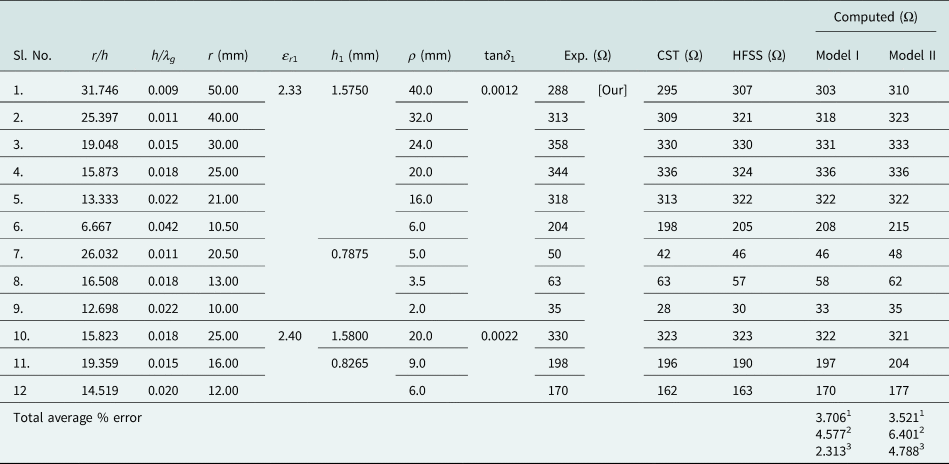
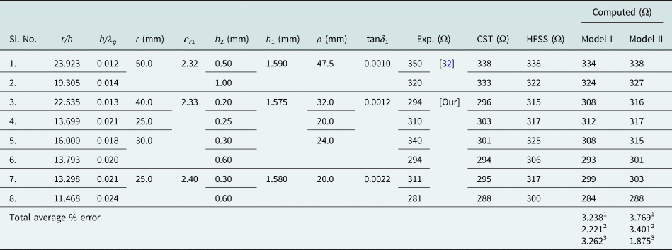
In Table 9, we have compared computed R employing the proposed models with our measured and measured values reported in [Reference Dahele, Mem and Lee32] along with simulation results (HFSS, CST) for a circular patch with variables h 2 and r/h. The total average % error shows that the present models accurately compute the input resistance at resonance.
Comparison of theoretically predicted dominant mode input resistance obtained from the present work for a circular microstrip patch with varying air gap, r/h, ɛr, h/λg with simulation (HFSS, CST) and new experimental results and experimental results from [Reference Dahele, Mem and Lee32]

ɛr 2 = 1.0.
‘1’ w.r.t Expt., ‘2’ w.r.t. CST, ‘3’ w.r.t. HFSS.
For the CST simulator, we have taken the frequency domain solver setting with S parameter error threshold value 0.01 and tetrahedral mesh properties by maximum cell per wavelength 10, per box edge 10. For HFSS, we have taken the solver setting by taking the number of passes 50, maximum delta S 0.02, fast sweep and frequency step size 0.001 GHz. Here, a personal computer having 2.80 GHz processor and 4GB RAM is used for simulation. Now, CST has taken around 9 and 7 min of time, respectively, to simulate circular patch antenna on two layers and a single layer, respectively. The HFSS has taken around 4 and 3 min to simulate those structures. But, the proposed models take only a fraction of a second to solve the same. So, the proposed models take lots of time faster than the simulators.
Radiation pattern
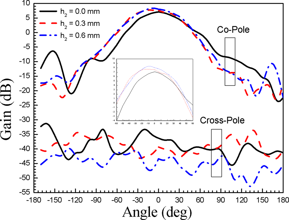
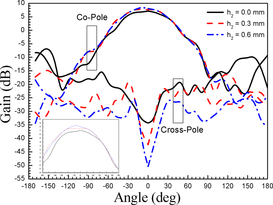
Figure 29 depicts the experimental E-plane co- and cross-polarized and Fig. 30 depicts the measured H-plane co- and cross-polarized gain pattern of a circular patch for three different h 2. The co-polarized peak gains for both planes increase with the increase of h 2. Whereas, cross-polarized peak gains for both planes are decreased with the increase of h 2.
Experimental variation of gain for different h. r = 25.0 mm, h 1 = 1.575 mm, ɛr 1 = 2.33, ɛr 2 = 1.0, tanδ 1 = 0.0012, tanδ 2 = 0.000, ρ = 6.0 mm: E-plane.

Experimental variation of gain for different h. r = 25.0 mm, h 1 = 1.575 mm, ɛr 1 = 2.33, ɛr 2 = 1.0, tanδ 1 = 0.0012, tanδ 2 = 0.000, ρ = 6.0 mm: H-plane.

Conclusion
This article presents two improved closed-form models for computing the fr, QT, B.W, D, G, XF, and Zin of a circular patch antenna excited by a coaxial probe. The presented models are based on the cavity model and parallel R-L-C circuit. The models are very simple and take very less time for implementation. The proposed models are directly applied in CAD programs. Here, we have employed a number of new expressions for determining the different performance parameters of a circular patch antenna. The presented models accurately calculate the performance parameters of a circular patch antenna for a wide range of variation of r/h, h/λg, and ɛr. The range of these variables are 2 ≤ r/h ≤ 100, 0.002 ≤ h/λg ≤ 0.22, and 2.2 ≤ ɛr ≤ 10.2. So, the proposed models are suitable for designing both electrically thick and thin substrate antenna. The models also accurately compute the input impedance and probe reactance for all probe location beneath the patch. A large number of experiments have been performed to verify the models. The presented models show that the total average percentage error for resonant frequency, probe reactance, input resistance, B.W, and gain is about 0.9, 3.5, 5, 6, and 4.5%, respectively, against the experimental results. We have also employed two commercial software to verify the models. For each structure, the HFSS takes 3–4 min, CST takes 7–9 min, whereas the proposed models take only a fraction of a second. Thus, the proposed models are ideal for the direct synthesis of circular disc antenna. The advantage of the structure is that we have achieved the frequency, bandwidth, and gain tunability without altering any antenna parameters.
 Manotosh Biswas was born in West Bengal, India, in 1976. He received his B.Tech., M.Tech., and Ph.D. degrees in Radio Physics and Electronics from the University of Calcutta, India, in 2001, 2003, and 2008, respectively. Dr. Biswas obtained the Young Scientist Award from URSI in 2005 and is a senior member of IEEE. He started his carrier in the Department of Electronics, West Bengal State University, India as a Reader in February 2009. In July 2010, he joined as a Reader in the Department of Electronics and Tele-Communication Engineering, Jadavpur University, India and currently he is serving as a Professor in the same university. His research interest includes planner antennas, dielectric resonator antennas, and metamaterials. He has published more than 29 technical journal articles and 49 technical conference proceedings articles.
 Mihir Dam was born in Kolkata, India, on January 1, 1983. He received the M.Sc. degree in Electronic Science in 2005 and the M.Tech. degree in Radio Physics and Electronics in 2007 from Calcutta University, India. He received the Ph.D. degree from Jadavpur University, India, in 2019. Currently, he is working as an Assistant Professor in the Department of Electronics, Vidyasagar College for Women. He has published more than seven technical journals and more than 15 technical conference articles. His research interest includes microstrip patch antennas, dielectric resonator antennas, etc.
 Sourav Banik was born in Kolkata, India, on November 7, 1987. He received the M.Sc. degree in Electronic Science in 2011 from the Department of Physics, Jadavpur University, India. He is currently working on his Ph.D. degree from the Department of Electronics and Telecommunications Engineering at Jadavpur University in the field of microstrip patch antennas. He has published more than four technical journals and more than seven technical conference articles.