INTRODUCTION
Plant photosynthesis provides the carbon and energy that drive most biological processes in an ecosystem. The photosynthetic model is the mathematical representation of photosynthesis and it is becoming highly valued in soil–vegetation–atmospheric interaction studies. It is generally known that parameter regionalization is the foundation of spatial application of a photosynthetic model at a canopy scale. Remote sensing (RS) improves the spatial application of the photosynthetic model greatly, by offering information on the spatial and temporal variability of important photosynthetic parameters that may be very difficult to obtain in situ.
The widely accepted, steady-state photosynthetic model proposed by Farquhar, von Caemmerer and Berry (FvCB) is detailed in Farquhar et al. (Reference Farquhar, Von Caemmerer and Berry1980). It summarizes the dependence of carbon (C) assimilation rate (A) on intercellular carbon dioxide (CO2) partial pressure (C i) as determined by saturation of Rubisco with respect to carboxylation (V cmax), electron transport as limited by ribulose bisphosphate (RuBP) regeneration (J max), or triose phosphate export. Coupled with a stomatal conductance model, often of the Ball-Berry (Ball et al. Reference Ball, Woodrow, Berry and Biggens1987) or Leuning (Leuning Reference Leuning1995) type, the FvCB model provides a more realistic description of the CO2 assimilation process. It gives a direct response to the environmental changes that couple the biochemical process and the physical process tightly in the land–atmosphere interaction of the model.
Although the FvCB model makes no attempt to treat all the steps in the photosynthetic process, as noted by Farquhar et al. (Reference Farquhar, von Caemmerer and Berry2001), it achieves a useful balance between mechanistic detail and mathematical simplicity. Owing to its excellent performance given by its simplicity and the growing availability of the required enzyme kinetic constants (Bernacchi et al. Reference Bernacchi, Portis, Nakano, von Caemmerer and Long2002), the FvCB model has been used for a wide range of studies, from analysing underlying C3 leaf biochemistry to predicting photosynthetic fluxes of ecosystems in response to global warming. Meanwhile, various modifications and improvements to the model have been developed in order to extend its application. For instance, because leaf physiological properties vary throughout the plant canopy in response to photosynthetically active radiation (PAR), the photosynthetic rate of an entire canopy can be estimated by multiplying the photosynthetic rate of the uppermost leaves in the canopy by the canopy PAR and the canopy extinction coefficient for PAR (Sellers et al. Reference Sellers, Los, Tucker, Justice, Dazlich, Collatz and Randall1996). Sellers’ work not only extends the application of the FvCB model to the canopy scale, but also establishes the foundation for a new area of couple satellite RS of spectral reflectance to estimate the absorbed PAR.
RS provides vegetation information at a large scale, which is widely used to scale up the ecosystem model integrated with the FvCB model. There are different ways to integrate the RS data with an ecosystem model, such as directly forcing and parameter estimation. As a critical indicator of vegetation condition, remote sensing leaf area index (LAI) is a variable used widely to drive the ecosystem models at the regional scale. Although the method of retrieving LAI from RS data has been improved in recent years (Haboudane et al. Reference Haboudane, Miller, Pattey, Zarco-Tejada and Strachan2004; Hasegawa et al. Reference Hasegawa, Matsuyama, Tsuzuki and Sweda2010), there are still two major difficulties in practice: (1) vegetation indices have definite limitations, which are not a single measure of a specific variable of interest (such as canopy architecture or pigment content) but depend on both the structural and biochemical properties of the canopy. Usually, vegetation indices approach their saturation levels asymptotically when the LAI exceeds 2–5 (Rautiainen Reference Rautiainen2005; Hasegawa et al. Reference Hasegawa, Matsuyama, Tsuzuki and Sweda2006). (2) There is no unique relationship between the LAI and a vegetation index of choice; a large number of relationships have been established, and a wide range of determination coefficients (0·05<R 2 < 0·66) between satellite-derived spectral indices and the LAI are found (Baret & Guyot Reference Baret and Guyot1991; Chen Reference Chen1996; Brown et al. Reference Brown, Chen, Leblanc and Cihlar2000).
The suitability of the FvCB model for describing fundamental responses of photosynthesis is such that V cmax and J max have become valuable metrics of photosynthetic performance in themselves. It is therefore vital to obtain accurate values for V cmax and J max in order to achieve good performance of the FvCB model. These two parameters are traditionally obtained by in situ measurements (Müller et al. Reference Müller, Wernecke and Diepenbrock2005; Alonso et al. Reference Alonso, Perez and Martinez-Carrasco2009). Recently, the quantitative relationship between these parameters and the RS data has just begun to be understood (Hu & Mo Reference Hu and Mo2011).
Many of the conditions that affect plant development and grain yield either favourably or adversely (i.e. fertilization treatment, rust infection, drought or precipitation events) result in a corresponding increase or reduction of the crop's photosynthetically active biomass at the canopy scale, and this response can often be captured though spectral measures such as the normalized difference vegetation index (NDVI) (Tucker Reference Tucker1979). However, the NDVI often fails to reflect plant photosynthetic capacity accurately, especially when the time of NDVI collection does not coincide with the period when the crop's photosynthetically active biomass is flourishing. Most authorities recommend collection of spectral data when the crop canopy is full (Lenney et al. Reference Lenney, Woodcock, Collins and Hamdi1996; Basnyat et al. Reference Basnyat, McConkey, Lafond, Moulin and Pelcat2004; Becker-Reshef et al. Reference Becker-Reshef, Vermote, Lindeman and Justice2010), because image acquisition before full crop canopy coverage results in spectral information that includes the contribution from the soil surface rather than from just the crop itself. Usually, the cumulative NDVI in the flourishing stage is a good indicator of plant photosynthetic capability (Basnyat et al. Reference Basnyat, McConkey, Lafond, Moulin and Pelcat2004), since it provides the aggregated assessment of plant photosynthetic capacity over time. In the present paper, regional V cmax pattern of winter wheat was derived from the model's predicted photosynthetic capacity through regressing the accumulated NDVI during the growing season and grain yield at the county level, with the assumption that the vegetation interface process (VIP) ecosystem model has good performance in yield simulation at regional scale (Hu & Mo Reference Hu and Mo2011)
The present paper compares simulated wheat yield and evapotranspiration (ET) by the VIP ecosystem model using the V cmax pattern (Hu & Mo Reference Hu and Mo2011) with the results obtained by the LAI method that used the retrieved LAI from the NDVI to drive the VIP model. Through the comparison, the intention was to explore (1) the consistency of the model performances in regional wheat yield and ET prediction with the two methods and (2) the source of simulation errors of the two methods.
MATERIALS AND METHODS
Region description
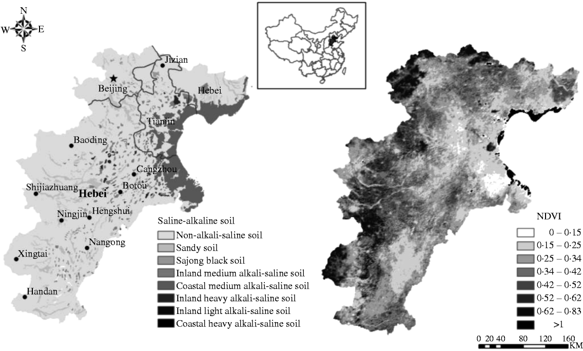
The Beijing–Tianjin–Hebei region is located in the northern part of the North China Plain (NCP), which covers Beijing, Tianjin and part of Hebei province (36°05′–40°24′N, 113°11′–119°45′E, 0–540 m asl). The prevailing cropping system is a wheat–maize rotation, which represents the traditional cropping system in the NCP and accounts for 0·9 of the cereal sowing area. The study area has a sub-humid warm temperate continental monsoon climate, with mean annual temperature of 10·8–14·1 °C and annual precipitation of 500–800 mm, which is distributed irregularly among the seasons. Approximately 0·75 of the rainfall occurs from late June to September during the maize growing season, and only 0·25 occurs in the wheat growing period from October to May. Therefore, most farmlands (c. 0·70) are irrigated fields. A part of the soil in this region is saline–alkaline soil (Fig. 1).
Geographical, saline–alkaline land map and NDVI of Beijing–Tianjin–Hebei region. The left map is Saline–alkaline land map; grey line is the province boundary. The right map is NDVI, 25 April 2002.

Model introduction
The VIP model used in the present study is a dynamic ecosystem model which simulates radiation, water, heat and CO2 transfer processes over the crop growing season (Mo & Liu Reference Mo and Liu2001; Mo et al. Reference Mo, Liu and Lin2012). It runs at a daily time-step using daily meteorological data, including daily average, maximum and minimum air temperature, atmospheric pressure, humidity, wind speed, precipitation and sunshine duration. The VIP model was used to simulate the biomass growth, grain yield and water balance of wheat in the double cropping system of the NCP.
The main biochemical processes in the VIP model include land surface energy balance, water cycle and carbon cycle, which have (1) a multi-layer canopy radiative transfer sub-model, (2) a canopy conductance/photosynthetic sub-model that distinguishes sunlit and shaded leaves, (3) a two-source soil-canopy energy balance sub-model, (4) a multi-layer soil water and heat transfer sub-model and (5) a crop growth module (Mo & Liu Reference Mo and Liu2001; Mo et al. Reference Mo, Liu, Lin and Zhao2004). Energy fluxes are described with a two-source scheme that discerns the canopy and soil surface separately. Transfer of solar radiation within the crop canopy is simulated with 20 sub-layers that distinguishes the direct and diffuse components of both the visible (300–700 nm) and near infrared (NIR, 700–1300 nm) fractions (Mo & Liu Reference Mo and Liu2001). The water cycle process deals with the total above-canopy ET and soil moisture transfer. The soil moisture budget is estimated using a six-layer scheme and described with Darcy's law (Hillel Reference Hillel1980). The carbon cycle includes assimilation via photosynthesis, crop growth and soil organic matter decomposition schemes. The daily growth of crop dry mass is expressed as the balance of gross photosynthesis, respiration and senescence (Mo et al. Reference Mo, Liu and Lin2012).
The present paper mainly concerns crop dry mass formation and water consumption of the C3 (wheat) crop. Energy transfer, the water cycle and the carbon cycle interact via ET, stomatal conductance and photosynthesis, and a detailed introduction to biochemical approaches for describing photosynthesis is given below.
The biochemical approaches to photosynthesis in the C3 crop according to Farquhar et al. (Reference Farquhar, Von Caemmerer and Berry1980), Collatz et al. (Reference Collatz, Ball, Grivet and Berry1991) and Sellers et al. (Reference Sellers, Los, Tucker, Justice, Dazlich, Collatz and Randall1996) have been employed in the present paper. The net assimilation rate of CO2 (A n, μmol C/m2/s) is expressed as
 $$A_n = \min (A_{\rm R}, A_{\rm E}, A_{\rm S} ) - R_{\rm d} $$
where A R is the Rubisco limiting rate, A E is the light-limited rate, A S is the capacity for the export or utilization of the products of photosynthesis, and R d is the leaf respiration rate (μmol C/m2/s). The Rubisco limiting rate, A R, is expressed as
 $$A_{\rm R} = V_{\rm c} \left[ {\displaystyle{{c_{\rm i} - \Gamma ^*} \over {c_{\rm i} + K_{\rm c} (1 + O_2 /K_{\rm o} )}}} \right]$$
where V c is Rubisco's maximum catalytic capacity (μmol C/m2/s), c i and O 2 are the intercellular concentrations of CO2 and O2 (Pa), respectively, Γ* is the CO2 compensation point (Pa = 0·5 O2/S, S is the Rubisco specificity for CO2 relative to O2), and K c and K o are Michaelis constants for CO2 and O2, respectively (Pa). In the VIP model, V c declines exponentially with an extinction coefficient, k v, and is expressed as
 $$V_{\rm c} = V_{{\rm c}\max} \exp ( - k_{\rm v} L)$$
where V cmax is the value of V c at the top of the canopy, k v is taken as 0·6 and L is the LAI which is determined by the leaf dry mass in the dynamic crop growth process. For more details about A E and A S, please refer to Mo & Liu (Reference Mo and Liu2001).
Daily crop dry matter production, denoted as M (mol C/m2/d), is expressed as the balance of gross photosynthesis, respiration and senescence in the vegetative stage, namely:
 $$\displaystyle{{{\rm d}M_{\rm i}} \over {{\rm d}t}} = \alpha _{\rm i} A_{\rm c} - R_{{\rm ci}} - R_{{\rm mi}} - D_{\rm i} $$
where i represents the stem (s), leaf (l) and root (r) fractions, respectively (therefore the equation was computed three times, once for each plant part), A c is the daily net photosynthesis (mol C/m2/d) at the canopy level determined by integrating the instantaneous A n values over daytime, and α is the partition coefficient (Arora & Boer Reference Arora and Boer2005), R c (mol C/m2/d) is the growth respiration, R m (mol C/m2/d) is the maintenance respiration and D (mol C/m2/d) is the senescence rate. The daily growth of LAI is determined by the daily dry mass allocated to the leaf and the specific leaf area (S LA m2g/c) (Eqn 5). Based on the results from the field tests in the study area, the specific leaf area is set as 0·07.
 $${\rm LAI} = S_{{\rm LA}} \times M_{\rm l} $$
Methods
Method of LAI retrieval from RS data (LAI method)
LAI is one of the most important variables governing canopy processes. It is related to the photosynthesis rate, the carbon and nutrient cycles, the biomass and crop growth stage (Herrmann et al. Reference Herrmann, Pimstein, Karnieli, Cohen, Alchanatis and Bonfil2011). As LAI is functionally linked to the canopy spectral reflectance, a common non-destructive surrogate for LAI is the NDVI, which is based on the reflectance of red (R) and NIR bands. However, there is a general agreement that a strong relationship exists between the fraction of absorbed PAR (F PAR) and the NDVI than that between the LAI and the NDVI (Myneni et al. Reference Myneni, Hall, Sellers and Marshak1995, Reference Myneni, Hoffman, Knyazikhin, Privette, Glassy, Tian, Wang, Song, Zhang, Smith, Lotsch, Friedl, Morisette, Votava, Nemani and Running2002). In the present study, F PAR is used to establish the link between the NDVI and LAI, and LAI is estimated by the following expression (Monteith & Unsworth Reference Monteith and Unsworth1990):
 $${\rm LAI} = {\rm LAI}_{\max} \displaystyle{{\ln (1 - F_{{\rm PAR}} )} \over {\ln (1 - F_{{\rm PAR}\max} )}}$$
where LAImax is the maximum LAI during the growing period (assumed to be 6·0), and F PAR is calculated as a linear relation of the NDVI (Sellers et al. Reference Sellers, Los, Tucker, Justice, Dazlich, Collatz and Randall1996):
 $$F_{{PAR}} = \displaystyle{{({NDVI} - {NDVI}_{\min} )(F_{{PAR}\max} - F_{{PAR}\min} )} \over {{NDVI}_{\max} - {NDVI}_{\min}}} $$
where NDVImax and NDVImin are the maximum and minimum NDVI, respectively, and F PARmax and F PARmin are the maximum and minimum F PAR corresponding to NDVImax and NDVImin, set as 0·95 and 0·001.
In the LAI method, the parameter V cmax is constant in the study area; the LAI is not controlled by leaf growth in the model but is estimated by the NDVI. The Terra-Modis 16-days NDVI are interpolated to daily time-step by the Lagrange interpolation method (Carrer & Mansur Reference Carrer and Mansur2006).
Method of V cmax retrieval from RS data (V cmax method)
The value of V cmax is affected by any factor that may affect the amount of activated enzyme (Rubisco) present, such as nitrogen limitation, insufficient irrigation and saline–alkaline soil. Under these environmental stresses, the chlorophyll content declines and induces a decline in the V cmax value. The chlorophyll content affects the properties of green vegetation to reflect the incident solar radiation, and this response can be detected by the NDVI value. Therefore, stressed vegetation or vegetation with low photosynthetic capability has reduced NDVI value (Basnyat et al. Reference Basnyat, McConkey, Lafond, Moulin and Pelcat2004), which means that the seasonal cumulative NDVI can be a good indicator of photosynthetic capability for specific vegetation. Meanwhile, plants with low photosynthetic capability produce less carbohydrate and have low crop yields. Since the crop yield and NDVI have an empirical relationship (Moriondo et al. Reference Moriondo, Maselli and Bindi2007; Ren et al. Reference Ren, Chen, Zhou and Tang2008), the regional V cmax pattern can be obtained from the NDVI through assimilating the RS NDVI and census data of grain yield at the county level into the ecosystem model (Hu & Mo Reference Hu and Mo2011).
In the V cmax method, the meteorological data, geographical data and the V cmax pattern are used to drive the VIP model. The pattern of the parameter V cmax used in the VIP model is estimated by the relationship between the NDVI and the V cmax; the LAI is controlled indirectly by the V cmax in the crop growth module. Therefore, NDVI is not used directly in the model, but only used to obtain the V cmax pattern. In the present study, the regional photosynthetic capability of the wheat was estimated by the relationship between NDVI and V cmax (Eqn 10) shown below, and the following steps were taken to deduce this relationship in the study region (Hu & Mo Reference Hu and Mo2011):
(1) Seeking the relationship between NDVI and crop yield
The linear relationship between yield and the NDVI is established by the cumulative NDVI data and the census data of grain yield. The census data is the county-level wheat yield data of the 104 counties in the study region in 2001, and the cumulative NDVI data is the corresponding county-level average value of cumulative NDVI from March to June in 2001. The regressive equation is expressed as follows:
(8)where y yield is the county-level yield of winter wheat, and x NDVI is the county-level average value of accumulative NDVI. $$y_{{yield}} = 747{\cdot}71x_{{NDVI}} + 2371{\cdot}40$$
(2) Seeking the relationship between V cmax and the crop yield by the VIP model
Different V cmax is used to drive the VIP model to obtain the simulated yield in Shijiazhuang, which is a typical area with wheat-maize rotation system in the NCP. The V cmax and the corresponding simulated yield data are used to establish the relationship between V cmax and yield, the regressive equation is expressed as follows:
(9)where y Vcmax is the value of V cmax, and x yield is the winter wheat yield.$$y_{Vc\max} = 17{\cdot}46e^{0{\cdot}0003x_{{yield}}} $$(3) Obtaining the relationship between V cmax and NDVI with the aid of crop yield.
Since the relationship between V cmax and yield is controlled by the mechanism of crop growth, the relationship between the yield and V cmax in Shijiazhuang can be scaled up to the study region. Based on the assumption that the VIP model has good performance in yield simulation at a regional scale, which means that the simulated yield is equal to the census data of grain yield, the relationship between V cmax and NDVI can be derived from the two equations above and is expressed as follows:
(10)where y Vcmax is the value of V cmax at each grid and x NDVI is the value of the accumulative NDVI at each grid.$$y_{Vc\max} = 17{\cdot}46e^{(0{\cdot}23x_{{NDVI}} + 0{\cdot}71)} $$



Data sources
Three types of data were used: geographical, meteorological and agricultural. Geographical data were used as the basic land surface information for the crop and soil, meteorological data were used as atmospheric forces to drive the VIP model and the agricultural data were used to validate the model and crop parameters.
Land surface characterization data and RS data
The land surface characterization data included the topography, land use map and soil maps. The digital elevation model was obtained from the topographic map at a 1 : 250 000 scale, which could be created using a terrain raster with a resolution as fine as 1 km.
Land use data were taken from the land use datasets developed by the Chinese Academy of Sciences from Landsat Thematic Mapper (TM) scenes with a spatial resolution of 30 × 30 m (Zhuang et al. Reference Zhuang, Liu and Liu1999; Liu et al. Reference Liu, Tian, Liu, Zhuang, Melillo and Zhang2005; datasets available online at http://www.resdc.cn/, accessed September 2010). The database includes time series data for three time periods: late 1980s, mid 1990s and late 1990s. The land use is classified into six types: farmland, mixed forest, grassland, urban land, water area and unutilized land (Liu et al. Reference Liu, Tian, Liu, Zhuang, Melillo and Zhang2005). In the present study, only farmland in the late 1990s which includes Landsat-TM scenes for 1999/2000 was taken into consideration, and the land use raster data with spatial resolution of 30 × 30 m was re-sampled to 1 × 1 km by the nearest neighbour resampling method (Parker et al. Reference Parker, Kenyon and Troxel1983).
The soil maps include a saline–alkaline land map and a soil physical texture map. In the saline–alkaline land map, the soil is divided into four types: inland alkali–saline soil, coastal alkali–saline soil, sandy soil and sajong black soil. The present paper was only concerned with the alkali–saline soil and the information was virtually retrieved from the resource's satellite images from the spring of 1978 to the spring of 1981 (Mo et al. Reference Mo, Liu, Lin and Guo2009). The soil physical texture data were retrieved from a 1 : 14 000 000 scale map (Institute of Soil Science, Academia Sinica 1986).
The RS data used in the present study were 16-day composite 1 km NDVI from 2001 to 2009. These data were sourced from the MOD13A2 NASA science data product (Huete et al. Reference Huete, Justice and van Leeuwen1999) and distributed by the Land Processes Distributed Active Archive Center (LP DAAC), located at the US Geological Survey (USGS) Earth Resources Observation and Science (EROS) Center. The land use mask derived from Landsat-TM image (http://www.resdc.cn/) was used to eliminate the influence of non-agricultural land on the NDVI signal. Consequently, all areas with non-agricultural land were masked out and NDVI values were extracted for only those areas having crops. Also excluded were all locations where the absolute range of values (maximum–minimum of the annual NDVI) was <0·1. The majority of these pixels usually indicated built-up areas. The locations where the NDVI values were beyond the scope of 0–1 were also excluded, because the majority of these pixels usually indicated surface water areas. The NDVI values obtained from satellite data can often be noisy due to persistent cloud cover over large regions. This is possible even when 16-day composited images are employed. Therefore, Savitzky–Golay filters (Chen et al. Reference Chen, Jonsson, Tamura, Gu, Matsushita and Eklundh2004) for reducing noise and constructing high-quality NDVI time-series data sets were applied.
All of the geographic information and RS images were processed for projection transformation (Lambert projection), and geometrical and atmospheric correction were used to remove the cloud effect (Kaufman & Tanre Reference Kaufman and Tanre1996).
Meteorological data
Using the inverse distance square method, the daily meteorological data were interpolated to the whole region with the meteorological data (1999–2009) from 88 meteorological stations in and around the NCP. These meteorological data, which were used to drive the model, included the daily average, maximum and minimum air temperature, atmospheric pressure, humidity, wind speed, precipitation and sunshine duration. With the exception of the sunshine duration, all of these variables were corrected with the elevation above sea level.
Agricultural data
The agricultural data included the ET of wheat in Luancheng Agricultural Experimental Station, the grain yield of winter wheat at the county scale of Beijing, Tianjin and Hebei province from 2001 to 2008 and the grain yield of winter wheat in three agricultural meteorological stations (Jinghai, Rongcheng and Zuozhou). The ET of wheat was measured by a large-scale weighting lysimeter (2001–8) in Luancheng Agricultural Experimental Station (37°51′–37°55′N, 114°39′–114°43′E), and can be obtained from Chinese Ecosystem Research Network (http://www.cerndata.ac.cn/). The census data of grain yield, taken from the China agricultural annals of 2002–9 and the provincial agricultural annals (Hebei Province Bureau of Statistics 2009), included the county-level yield data of 104 counties from 2001 to 2008. The grain yield of winter wheat at the agricultural meteorological stations can be downloaded from the China Meteorological Data Sharing Service System (CMDSSS, http://cdc.cma.gov.cn/index.jsp).
Model runs
The growth process of winter wheat was simulated from 1999 to 2009 using a daily step and a 1 km grid over the study area. The model initialization period was performed from January 1999 to September 2000, with simulation results from 2001 to 2009 being used in the analysis. Because the exact irrigation amounts were unavailable over the study area, average irrigation amount was set as 11 October, 25 March, 15 April and 5 May in each year with 60 mm of water each time, according to the most popular and traditional irrigation systems from the average of local information collected. When the LAI is estimated by the NDVI, the uniform parameter V cmax is set as 110 μmol C/m2/s for the running of the model. When the model is driven by the V cmax pre-defined pattern, the LAI is calculated by the crop growth module.
RESULTS
Validation of the different methods
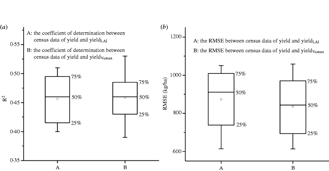
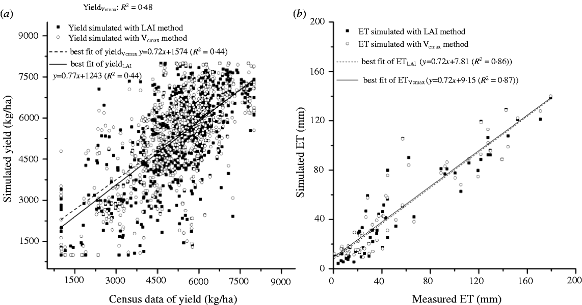
The results obtained when validating the LAI method and the V cmax method with the county-level grain yield of each year from 2001 to 2008 are shown in Fig. 2. Better performance was obtained when using the V cmax method, with an average coefficient of determination (R 2) of 0·46 and an average root mean square error (RMSE) of 836 kg/ha (which was c. 0·17 of the census data of grain yield). The RMSE of the LAI method (872 kg/ha), which was 0·20 of the census data of grain yield, was a little higher than that of the V cmax method, despite the similarity in the average R 2 of the LAI method (0·45) and the V cmax method. The relationships between the census data of grain yield and the yields simulated by the two methods from 2001 to 2008 (taken as one dataset of 8 years) are shown in Fig. 3(a). Similar linear fits were obtained via the two methods with the same R 2 (0·44). These results indicated that the county-level yields simulated by the V cmax method were more reliable than those simulated by the LAI method, although both methods give satisfactory performance.
Box plots of (a) correlation coefficients and (b) RMSE between simulated yield and census data of yield from 2001 to 2008. The squares inside the boxes correspond to the mean value and the whiskers extend to the minimum and maximum values.
Cross plots of (a) county-level simulated yield and census data of yield and (b) comparison of simulated and observed monthly ET in Luancheng Agricultural Experimental Station from 2001 to 2008.
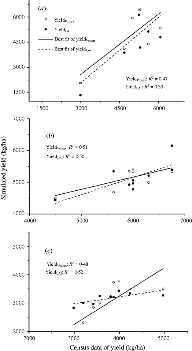
Given that the spatial variability of some factors affecting the yield may be ignored when utilizing the county-level grain yield to verify the simulated ones, some plot-level field data were picked out for verification. Since water stress is one of the main factors that limit crop yield and result in spatial variation, the validation results for irrigated fields (Rongcheng and Zuozhou) and rain-fed fields (Jinhai) are shown in Fig. 4. Although the simulated values of both methods agreed reasonably well with the field data, the R 2 between the simulated and the measured yield in the V cmax method was higher than that of the LAI method in the irrigated fields (Figs 4(a) and (b)), whereas the opposite was seen in the rain-fed fields (Fig. 4(c)). This indicates that the V cmax method only performs better than the LAI method for irrigated fields. For ET, both ET simulated with the LAI method (ETLAI) and ET simulated with the V cmax method (ETVcmax) were in good agreement with the measured ET, with R 2 of 0·86 for ETLAI and 0·87 for ETVcmax (Fig. 3(b)), indicating that there was little discrepancy between the two methods.
Cross plots of simulated yield and census data of yield of (a) Rongcheng (irrigated field), (b) Zuozhou (irrigated field) and (c) Jinghai (rain-fed field).
The above comparisons (yieldLAI and yieldVcmaxv. census data of yield, ETLAI and ETVcmaxv. measured ET) demonstrated that the performance of the V cmax method was similar to that of the LAI method in the whole study area and even better in irrigated fields.
Comparisons of the performance of the different methods
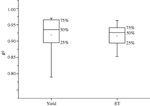
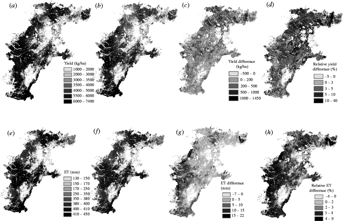
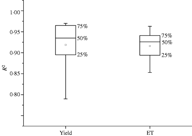
As the yield and seasonal ET simulated by the V cmax method correlated strongly with those of the LAI method, with R 2 ranging from 0·79 to 0·97 (0·85–0·96 for ET) (Fig. 5), the spatial variation of the yield and ET with the V cmax method was highly consistent with those of the LAI method (Fig. 6). However, there are two differences between the two patterns, namely the distribution frequency of the yield and ET and the area of field with high productivity and ET.
Box plots of determination coefficients of simulated results between V cmax method and LAI method from 2001 to 2009. The squares inside the boxes correspond to the mean value and the whiskers extend to the minimum and maximum values.
Maps of average simulated wheat yield and ET from 2001 to 2009. (a) yield simulated by the V cmax method (yieldVcmax), (b) yield simulated by the LAI method (yieldLAI), (legend of this map is the same as (a)), (c) yield difference between the V cmax method and LAI method (yieldVcmax minus yieldLAI), (d) relative yield difference between the V cmax method and the LAI method (yield difference divided by yieldLAI), (e) ET simulated by the V cmax method (ETVcmax), (f) ET simulated by the LAI method (ETLAI), (legend of this map is the same as (e)), (g) ET difference between the V cmax method and LAI method (ETVcmax minus ETLAI); (h) relative ET difference between the V cmax method and LAI method (ET difference divided by ETLAI).
Figure 6(c) displays the spatial variation of the yield difference (yield simulated by the V cmax method minus that by the LAI method) between the two methods. The pixels with high values mostly appear at highly productive fields, indicating that large differences between the yields simulated by the two methods appeared at the highly productive fields with higher LAI. The spatial pattern of the relative yield difference (yield difference divided by yieldLAI) in Fig. 6(d) is similar to that of the yield difference in Fig. 6(c) in most parts of the study area except in a few parts with low productivity fields. In these low productivity fields, the yield differences between the two methods (not more than 500 kg/ha) and the yield (not more than 3000 kg/ha) were both small, which caused the relative yield difference to be quite high (more than 0·1). The same phenomenon was also found in the pattern of ET difference (ET simulated by the V cmax method minus that by the LAI method) shown in Fig. 6(g) and the relative difference of the ET pattern (ET difference divided by ETLAI) shown in Fig. 6(h), which demonstrated that large differences between the two methods in simulating yield and ET also appeared in some low productivity fields due to the poor accuracy of the inter-annual yield and ET estimated with the V cmax method.
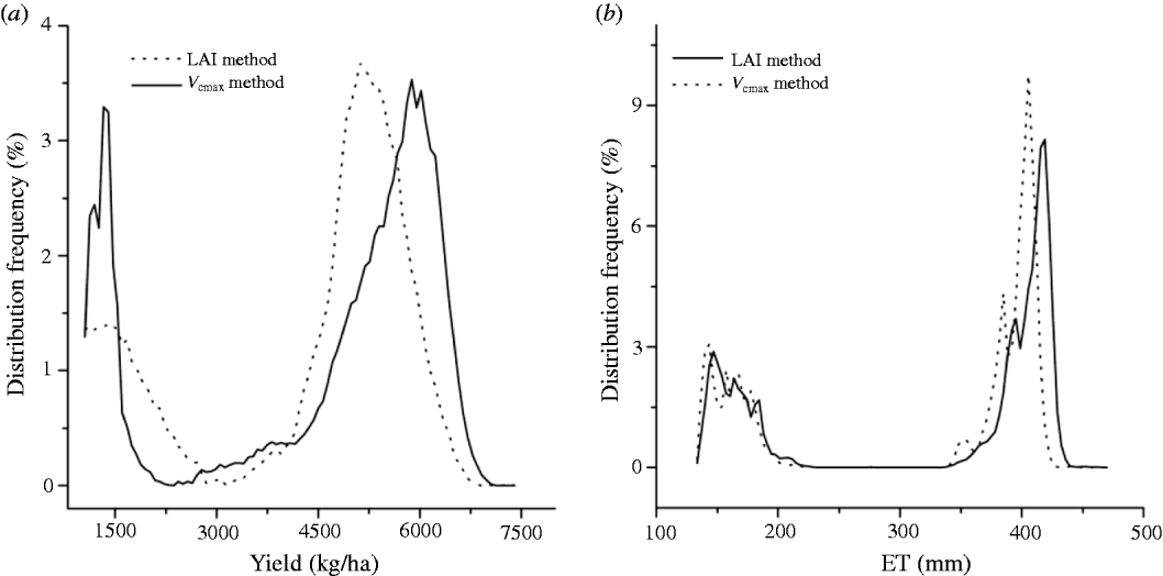
With respect to the difference of the two methods, the frequency distribution map provides a clearer picture than the spatial map. The yield data of the study area showed an interesting bimodal distribution corresponding to the rain-fed and irrigated fields, respectively. For the LAI method, the simulated yield ranged from 1000–7400 kg/ha, with the maximum frequency distribution at 1500 and 5200 kg/ha in the rain-fed and irrigated fields, respectively. For the V cmax method, the yield ranged from 1000 to 7200 kg/ha, with the maximum frequency distribution at the same yield level (1500 kg/ha) in the rain-fed field and 5900 kg/ha in the irrigated fields (Fig. 7(a)). The area of highly productive fields with yields of over 6000 kg/ha was larger for the V cmax method than the LAI method (Figs 6(a) and (b)). Further, the average simulated yield was higher for the V cmax method (4730 kg/ha) than that of the LAI method (4520 kg/ha). A similar frequency distribution pattern also appeared in the simulated ET (Fig. 7(b)). The simulated ET with the maximum frequency distribution for the V cmax method (420 mm) was higher than that for the LAI method (400 mm). This demonstrated that the area with more than 350 mm seasonal ET with the V cmax method was larger than that for the LAI method (Figs 6(e) and (f)), and the average seasonal ET simulated by the V cmax method (372 mm) was higher than that of the LAI method (360 mm) in the study area.
Distribution frequency of (a) average simulated wheat yield and (b) ET with V cmax method and LAI method.
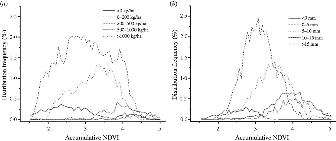
Based on the division standard used in (Figs 6(c) and (g)), the frequency distributions of the cumulative NDVI are shown in Fig. 8. As most pixels belong to the lowest difference level (0–200 kg/ha in yield difference and 0–5 mm in ET difference), there were no significant differences in the estimates of yield and ET between the two methods in most parts of the study area. The value of the cumulative NDVI with the maximum frequency distribution increased with the growth of yield difference and ET difference, indicating that the highly productive fields had remarkable differences in yield and ET simulation between the two methods.
Distribution frequency of cumulative NDVI at (a) five yield difference levels and (b) five ET difference levels.
Simulation errors of the LAI method and V cmax method
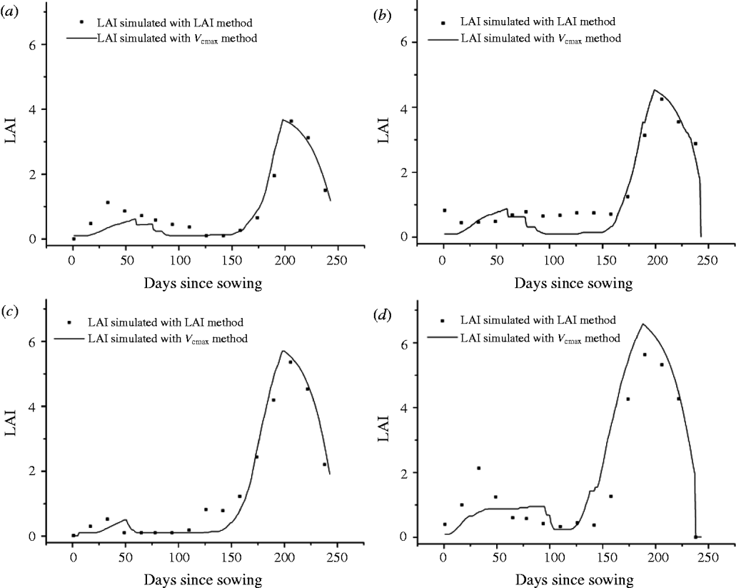
Because the NDVI saturates at high LAI values, the use of RS data introduces simulation errors in the LAI estimation. Comparing the variations of the LAI simulated by the two methods during the growth stage reveal that the underestimation of the LAI appears after the jointing stage (April) and reaches the peak at the heading stage (mid-May) (Fig. 9). At low photosynthetic capability levels (40–60 μmol C/m2/s), the difference in the LAI value is no more than 0·05. When the photosynthetic capability reaches 100–120 μmol C/m2/s, the maximum LAI value is 5·6 with the LAI method but up to 7 with the V cmax method. The V cmax method is closer to the measured value at the high photosynthetic capability levels.
Dynamic variation of average LAI during the growing season for the four V cmax value levels (a) 40–60, (b) 60–80, (c) 80–100 and (d) 100–120 μmol C/m2/s.
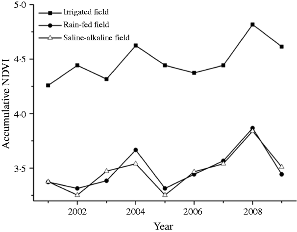
The NDVI has been proved to be a good indicator of the biomass and yield and a useful indirect tool for the evaluation of yield prediction with the two methods. The inter-annual variations of the mean cumulative NDVI values (March–June) in the irrigated fields, rain-fed fields and saline–alkaline land are shown in Fig. 10. Although the mean cumulative NDVI value in the irrigated field (4·48) is higher than that in the rain-fed field (3·49) and the saline–alkaline land (3·47), the standard deviation (SD) of cumulative NDVI in the irrigated field (0·174) is lower than that in the rain-fed field (0·186) and the saline–alkaline land (0·188), indicating that the inter-annual environmental variability in the rain-fed field and saline–alkaline land is more significant than those in the irrigated field.
Inter-annual variation of average accumulative NDVI (March–June) in the irrigated field, rain-fed field and saline–alkaline field.
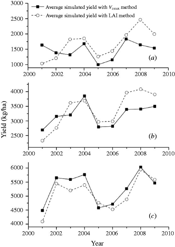
In the irrigated field, the yield simulated by the V cmax method and the LAI method showed a similar trend of annual variation (Fig. 11(c)). The correlation coefficient between the cumulative NDVI and yieldLAI (0·78) is similar to that between the cumulative NDVI and yieldVcmax (0·83). However, the yield in rain-fed field and saline–alkaline land appear as an increasing trend after 2007 in the LAI method, differing from the results in the V cmax method (Figs 11(a) and (b)).The correlation coefficient between the cumulative NDVI and yieldLAI (0·82 in the rain-fed field and 0·76 in the saline–alkaline land) is higher than that between the accumulative NDVI and yieldVcmax (0·59 in the rain-fed field and 0·55 in the saline–alkaline land). This illustrates that both the LAI method and the V cmax method can describe the inter-annual variability of yield in the irrigated field, but in the rain-fed field and the saline–alkaline field, the V cmax method shows more simulation errors and worse performance.
Inter-annual variation of average yield in the (a) rain-fed field, (b) saline–alkaline field and (c) irrigated field.
DISCUSSION
There are several sources of simulation error in the crop yield and ET simulation by the two methods. For the LAI method, the VIP model is driven by the LAI retrieved from NDVI. However, many studies illustrate that the NDVI will be saturated when the LAI value is larger than four, which results in an underestimation of the LAI at full canopy closure (Duchemin et al. Reference Duchemin, Hadria, Erraki, Boulet, Maisongrande, Chehbouni, Escadafal, Ezzahar, Hoedjes, Kharrou, Khabba, Mougenot, Olioso, Rodriguez and Simonneaux2006; Smith et al. Reference Smith, Bourgeois, Teillet, Freemantle and Nadeau2008). Although an estimation of the LAI from RS data may not be obtained by a uniform relationship, after assessing four LAI estimation approaches (stepwise multiple regression method, calibration and validation procedures, neural network based method and exponential law based method), Bsaibes et al. (Reference Bsaibes, Courault, Baret, Weiss, Olioso, Jacob, Hagolle, Marloie, Bertrand, Desfond and Kzemipour2009) reported that even in the best-performing approach, saturation problems were still observed for LAI values larger than four because of the saturation of the RS signal over the optical domain. In the present paper, the underestimation of the LAI appears after the jointing stage (April) and reaches the peak at the heading stage (mid-May). The maximum LAI value estimated by the V cmax method is closer to the measured value in the study area (Yang et al. Reference Yang, Watanabe, Zhang, Zhang, Wang and Hayashi2006; Li et al. Reference Li, Nielsen, Yua, Mac and Ahuja2010) than that by the LAI method, especially when the photosynthetic capability reaches 100–120 μmol C/m2/s, indicating that the LAI underestimation is more obvious at high photosynthetic capability levels in the LAI method. In contrast, when using the V cmax pattern to simulate the crop yield, the LAI is simulated by the ecosystem model, and the maximum leaf area is controlled by the functional mechanism of crop growth. This makes the LAI in the flourishing growth stage close to the true value and avoids the saturation problems to a given extent.
The LAI correlates significantly with plant biomass (Ozalkan et al. Reference Ozalkan, Sepetoglu, Daur and Sen2010) and yield (Murphy et al. Reference Murphy, Dawson and Jones2008), especially at the jointing stage (Moragues et al. Reference Moragues, del Moral, Moralejo and Royo2006). Combined with plant height, the LAI is responsible for 0·38 of the variation in yield (Moragues et al. Reference Moragues, del Moral, Moralejo and Royo2006). The underestimation of LAI in the flourishing stage results in underestimation of the seasonal ET and yield in the LAI method. In contrast, LAI underestimation is avoided effectively in the V cmax method at the crop flourishing stage by tracing the phenological processes of leaf growth. This makes the average yield and seasonal ET estimated by the LAI method lower than that estimated by the V cmax method.
The V cmax value is affected by any factors which may affect the amount of activated enzyme (Rubisco) present. Its average value is affected by the degree of environmental stresses, such as available nitrogen (Makino Reference Makino2003; Bruck & Guo Reference Bruck and Guo2006), heavily salinized soil and groundwater (Tester & Davenport Reference Tester and Davenport2003; James et al. Reference James, Munns, Von Caemmerer, Trejo, Miller and Condon2006). These environmental stresses will result in inter-annual variations of the V cmax pattern. Hence the V cmax method, which uses the V cmax value calculated by cumulative NDVI of a particular year, will give rise to errors in yield simulation, especially in areas with large environmental changes, such as the rain-fed field and saline–alkaline land. The present work shows that the correlation coefficient between the cumulative NDVI and yieldLAI in the rain-fed fields and saline–alkaline soils was higher than that between the accumulative NDVI and yieldVcmax, yet the correlation coefficient between the cumulative NDVI and yieldLAI in the irrigated field was similar to that between the cumulative NDVI and yieldVcmax. This illustrates that both the LAI method and the V cmax method can describe the inter-annual variability of the yield in irrigated fields, but in rain-fed fields and saline–alkaline lands, the V cmax method shows more simulation errors and worse performance due to a lack of concern for the expression of the inter-annual environmental change.
The main conclusions are that both the V cmax method and the LAI method give satisfactory results in estimation of yield and ET at a regional scale. However, the V cmax method avoids the saturation problem in highly productive areas. Therefore, both yield and ET simulated with the V cmax method are higher than that with the LAI method, and the fraction of field with a high yield in the V cmax method is larger than that in the LAI method. In low productivity fields, the V cmax method cannot describe the dramatic inter-annual variability of crop productivity and introduces larger errors in yield simulation than the LAI method.
This study was jointly supported by the Natural Science Foundation of China (NSFC) grants (31171451), the Chinese Ministry of Science and Technology Projects (2010CB428404) and the Key Project for the Strategic Science Plan in IGSNRR, CAS (2012ZD003). We thank the anonymous reviewers and the editors of the journal for their comments that improved an earlier draft of this paper.