






1 Introduction
The problem of the flow passing through a circular aperture in a plate is encountered in many practical applications, such as for example fuel injectors, cooling system for gas turbines or wind instruments. When subjected to harmonic forcing, for instance under the effect of an incident acoustic wave, the vortex sheet formed at the rim of the aperture becomes periodically modulated and acts as a spatial amplifier of Kelvin–Helmholtz instability, reorganizing the jet into an array of vortex rings. This feature is an essential part of the sound production mechanism in situations where the jet subsequently passes through a second aperture, a configuration known as ‘hole tone’ and encountered for instance in tea kettles (Henrywood & Agarwal Reference Henrywood and Agarwal2013) and bird calls (Fabre et al. Reference Fabre, Bonnefis, Charru, Russo, Citro, Giannetti and Luchini2014). The generation of vorticity is also an efficient mechanism to dissipate the acoustic energy. As a consequence, the use of multiply perforated plates traversed by a mean flow (or bias flow) is widely used as a sound attenuator device in many industrial applications, such as combustion system (Hughes & Dowling Reference Hughes and Dowling1990; Rupp, Carrotte & Macquisten Reference Rupp, Carrotte and Macquisten2012).
The unsteady, periodic flow through a circular hole in a zero-thickness plate was initially solved by Rayleigh (Reference Rayleigh1945) using inviscid, potential theory. The key result of his solution is the proportionality between the net pressure force felt from both sides of the hole and the acceleration of the fluid, so that the whole situation can be modelled by assuming that there is a rigid plug of fluid, with area
 $A_{h}=\unicode[STIX]{x03C0}R_{h}^{2}$
and equivalent length
 $\ell _{eff}$
, oscillating across the aperture, where
 $R_{h}$
is the radius of the hole.
The case where the flow has a mean component (or bias flow) in addition to the oscillating component was considered by Howe (Reference Howe1979). He introduced a key quantity, the Rayleigh conductivity
 $K_{R}$
, defined as the ratio of the acceleration of the fluid particles located within the aperture to the net force exerted on it. The real part of the conductivity generalizes the concept of equivalent length
 $\ell _{eff}$
previously introduced by Rayleigh, while its imaginary part is directly proportional to the flux of energy transferred from the imposed oscillatory flow to the jet. Under the hypothesis of high Reynolds number, low Mach number and assuming that the oscillating flow is of small amplitude with respect to the mean (or bias) flow, Howe derived a theoretical model describing the vorticity shed at the rim of the aperture and predicting the real and imaginary parts of the conductivity by analytical formulas. The main features and caveats of Howe’s model will be reviewed in § 2.5.
In recent years, a number of studies have considered the interaction between acoustics and perforated plates in more complex situations including multiple holes (Hughes & Dowling Reference Hughes and Dowling1990), turbulent flows (Tam & Kurbatskii Reference Tam, Christopher and Kurbatskii2000; Eldredge, Bodony & Shoeybi Reference Eldredge, Bodony and Shoeybi2007), acoustic liners formed by a honeycomb network of cavities (Mann et al. Reference Mann, Perot, Kim and Casalino2013; Zhang & Bodony Reference Zhang and Bodony2016) and slit resonators (Tam et al. Reference Tam, Ju, Jones, Watson and Parrott2005). However, in the applications targeted by these works, the mean flow is mostly tangential to the plate (grazing flow) and not across the hole. Coming back to situations where the holes are traversed by a mean flow (bias flow), in cases where the thickness of the hole is not small compared to its radius, experimental measurements of the impedance (Su et al. Reference Su, Rupp, Garmory and Carrotte2015) substantially deviate from Howe’s predictions, and a number of studies have proposed improvements of the original model to enlarge its range of validity (Jing & Sun Reference Jing and Sun2000; Bellucci et al. Reference Bellucci, Flohr, Paschereit and Magni2004; Yang & Morgans Reference Yang and Morgans2017). In the case where the amplitude of the oscillating flow becomes comparable to that of the mean flow, nonlinearities also lead to substantial deviations (Jing & Sun Reference Jing and Sun2002; Scarpato Reference Scarpato2014). However, in the case of small-amplitude oscillations and short holes, Howe’s model still constitutes the cornerstone for theoretical modelling of such flows (Scarpato et al. Reference Scarpato, Tran, Ducruix and Schuller2012).
In view of the above discussed literature, we can note that all available theoretical models are of inviscid nature and describe the vorticity production in terms of vortex sheets, thus these models are expected to be relevant only in the large Reynolds number limit. An alternative way, which allows us to incorporate viscous effects in a rigorous way and to consider arbitrary values of the Reynolds number, is to use linearized Navier–Stokes equations (LNSE). A number of studies have considered jet flows under this framework. Garnaud et al. (Reference Garnaud, Lesshafft, Schmid and Huerre2013) considered the spatial amplification properties of an incompressible jet using a laminar base-flow solution for
 $Re\leqslant 1000$
. Even more recent works have considered the case of compressible jets for
 $Ma\approx 0.9$
in the turbulent range (
 $Re\approx 10^{6}$
) using a mean flow obtained from experimental results (Semeraro et al.
Reference Semeraro, Lesshafft, Jaunet and Jordan2016), Reynolds-averaged Navier–Stokes (RANS) simulations (Jeun, Nichols & Jovanović Reference Jeun, Nichols and Jovanović2016) or large-eddy simulations (LES) (Schmidt et al.
Reference Schmidt, Towne, Colonius, Cavalieri, Jordan and Brès2017, Reference Schmidt, Towne, Rigas, Colonius and Brès2018). However, the focus of these studies was to characterize the spatial amplification properties of the jet and the sound radiation in the downstream domain due to vortex-shedding effects, which are different questions to the one we are considering here.
It should also be noted that the application of LNSE to jet flows is much more difficult for the high Reynolds number, laminar range
 $Re\approx [500-5000]$
which is considered in this paper than for the turbulent range. In effect, in the laminar range, the shear layers bounding the jet remain very sharp far downstream, leading to strong amplifications of convective instabilities extending very far away. It is thus difficult to design a method capturing both the spatial growth of perturbations in the axial direction, which can reach huge levels when the axial distance and the Reynolds number are large, and the coupling between the flow rate and the pressure jump, which is relevant when considering the possible coupling with an acoustical system. On the other hand, in the turbulent range, the shear layers of the jet spread rapidly in the downstream direction, leading to stabilization of the convective instabilities within a distance of approximately ten diameters of the jet.
The objectives of the present paper can thus be summarized in three main points.
(i) First, we wish to design a numerical approach based on the linearized Navier–Stokes equations, to compute the Rayleigh conductivity of the flow through a hole in the laminar but high Reynolds number range. We will introduce a convenient method based on a change of variable of the axial coordinate
 $x$
in the complex plane (inspired by the perfectly matching later method used in linear acoustics) which allows us to perform accurate computations up to
$Re\approx 10^{4}$
.
(ii) Secondly, we wish to reconsider the case of a hole of zero thickness initially investigated by Howe. We document the structure of base flow, with particular focus on the vena contracta phenomenon. We then describe the spatial structures corresponding to the linear response of the jet to harmonic forcing. The velocity and vorticity components of these structures allow us to describe the spatial amplification by the jet, while the pressure components give access to the Rayleigh conductivity. We will compute and display the Rayleigh conductivities (as well as the equivalent concept of impedance) as functions of forcing frequency and Reynolds number in the range
$10^{2}$
–
$10^{4}$
and compare with the inviscid predictions of Howe.(iii) Finally, the third objective is to assess the validity of the linearized Navier–Stokes equations with respect to perturbations of finite amplitude
$\unicode[STIX]{x1D700}$
. For this purpose, we will conduct a direct numerical simulation (DNS) of the forced axial–symmetric Navier–Stokes equations in the range
$\unicode[STIX]{x1D700}=$
[
$10^{-4}$
–
$10^{-1}$
]. Results show that the impedances are effectively well predicted by linearized Navier–Stokes equations (LNSE) up to
$\unicode[STIX]{x1D700}=10^{-1}$
, despite the fact that the evolution of vorticity perturbations in the jets are strongly nonlinear.


As briefly discussed in the bibliographical review, in the case where the plate is not thin and the holes are sufficiently long, different mechanisms take place and the jet can cease to act as a sound damper to become a sound generator (Jing & Sun Reference Jing and Sun2000; Yang & Morgans Reference Yang and Morgans2017). The conductivity/impedance concepts are useful tools to characterize the mechanisms in this case. A full characterization of the impedance of finite-thickness holes using the method introduced here as well as a discussion of impedance-based instability criteria will be presented in a forthcoming paper.
2 Problem definition and review of inviscid models
2.1 Problem definition
The situation considered here is the flow of a viscous fluid of density
 $\unicode[STIX]{x1D70C}$
and viscosity
 $\unicode[STIX]{x1D708}$
through a circular hole or radius
 $R_{h}$
and area
 $A_{h}=\unicode[STIX]{x03C0}R_{h}^{2}$
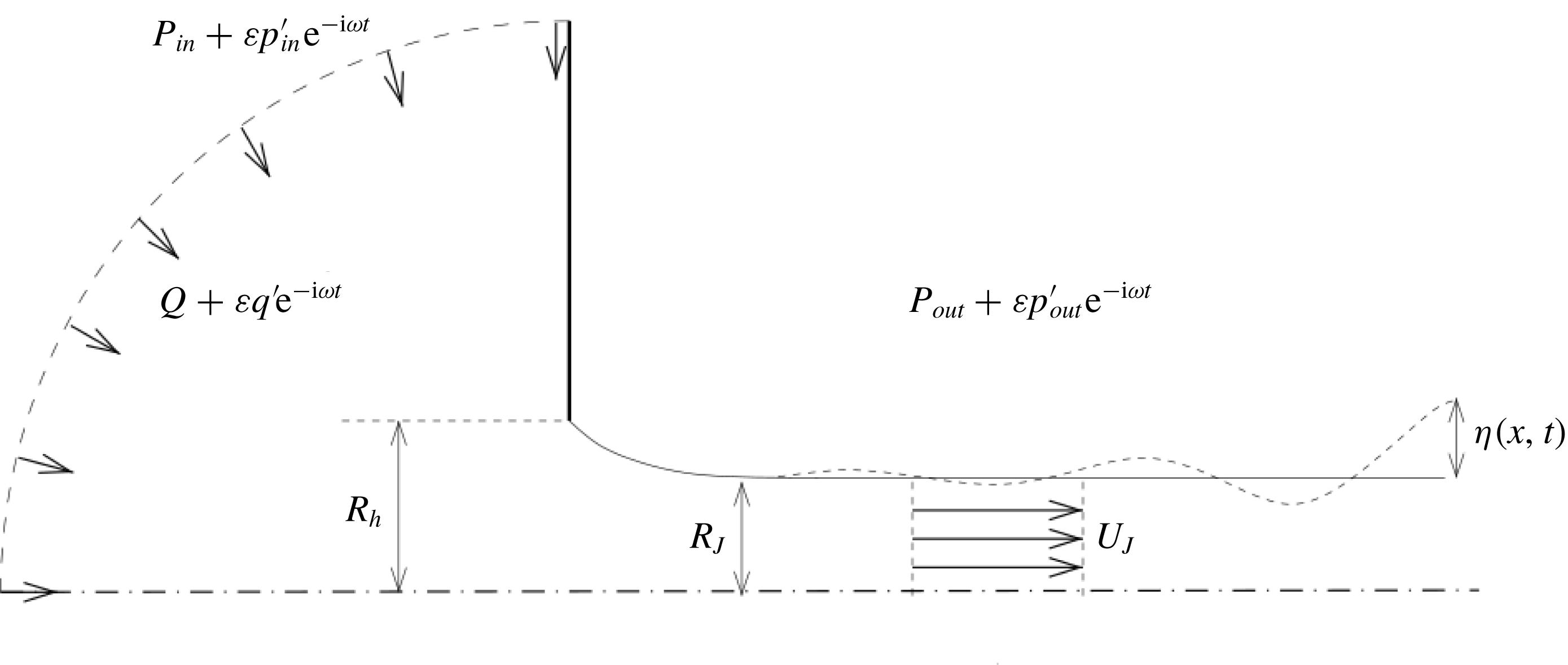
inside a planar thin plate of a thickness that is negligible with respect to the radius, connecting an inner and an outer open domain, as shown in figure 1. We note by
 $Q$
the mean volumetric flow rate across the aperture, and from that latter quantity we classically define the mean velocity as
 $U_{M}=Q/A_{h}$
. Thus the Reynolds number of the flow is defined as:
 $$\begin{eqnarray}Re=\frac{2R_{h}U_{M}}{\unicode[STIX]{x1D708}}\equiv \frac{2Q}{\unicode[STIX]{x03C0}R_{h}\unicode[STIX]{x1D708}}.\end{eqnarray}$$
When subjected to harmonic forcing with frequency
 $\unicode[STIX]{x1D714}$
, a second dimensionless parameter naturally emerges: the dimensionless frequency
 $\unicode[STIX]{x1D6FA}$
(or Strouhal number) defined as:
 $$\begin{eqnarray}\unicode[STIX]{x1D6FA}=\frac{\unicode[STIX]{x1D714}R_{h}}{U_{M}}.\end{eqnarray}$$
The final goal of our study is to characterize the interaction of the jet with acoustic waves, and in the general case this calls for a description using compressible equations. However, in many situations, it is justified to consider that the flow is locally incompressible, and hence to assume a uniform density
 $\unicode[STIX]{x1D70C}$
of the fluid. This simplification is justified under two hypotheses. First, the Mach number
 $Ma=U_{M}/c_{0}$
based on the mean velocity of the jet must be small enough. Secondly, all length scales charactering the aperture (here, the only relevant one is the radius
 $R_{h}$
since the thickness is assumed to be zero) have to be small compared to the acoustic wavelength
 $\unicode[STIX]{x1D706}_{ac}=2\unicode[STIX]{x03C0}c_{0}/\unicode[STIX]{x1D714}$
. This latter hypothesis is often referred to in acoustic textbooks as the acoustic compactness hypothesis. In dimensionless terms, the hypothesis can be formulated as
 $\unicode[STIX]{x1D706}_{ac}/R_{h}=2\unicode[STIX]{x03C0}/(Ma\unicode[STIX]{x1D6FA})\gtrsim 10$
, so for the largest frequencies considered here (
 $\unicode[STIX]{x1D6FA}\approx 6$
) it is valid up to
 $Ma\approx 0.1$
. For a flow of air through a typical hole of radius
 $R_{h}=1~\text{mm}$
, the condition
 $Ma\approx 0.1$
corresponds to
 $Re\approx 4500$
, confirming the relevance of the range of parameters investigated in the present paper.
Sketch of the oscillating flow through a circular aperture in a thin plate.
Under these two hypotheses, it is justified to assume that, far away from the hole, the pressure levels in the upstream and downstream regions tend to uniform values noted respectively by
 $p_{in}(t)$
and
 $p_{out}(t)$
. In the harmonic regime, the upstream and downstream pressure levels as well as the flow rate will be expanded as:
 $$\begin{eqnarray}\left(\begin{array}{@{}c@{}}p_{in}(t)\\ p_{out}(t)\\ q(t)\end{array}\right)=\left(\begin{array}{@{}c@{}}P_{in}\\ P_{out}\\ Q\end{array}\right)+\unicode[STIX]{x1D700}\left(\begin{array}{@{}c@{}}p_{in}^{\prime }\\ p_{out}^{\prime }\\ q^{\prime }\end{array}\right)\text{e}^{-\text{i}\unicode[STIX]{x1D714}t}+\text{c.c.},\end{eqnarray}$$
where
 $\unicode[STIX]{x1D700}$
is a given amplitude of the harmonic perturbation and
 $\unicode[STIX]{x1D714}\in \mathbb{R}$
is the oscillation rate. The interaction of the jet with external systems can thus be characterized by the sole relationship between the pressure drop
 $[\,p_{in}^{\prime }-p_{out}^{\prime }]$
and the flow rate
 $q^{\prime }$
of the harmonic part.
Ultimately, if one wants to introduce the jet in the description of an acoustic system of much larger dimensions, the description (2.3) can be matched with an external solution derived from the equations of acoustics. Such a matching is not conducted here but examples will be given in a forthcoming paper.
2.2 Steady flow
The steady flow corresponding to the present situation is globally characterized by the mean pressure drop
 $[P_{in}-P_{out}]$
and the mean flow rate
 $Q$
. In the inviscid case, a classical model to relate these quantities was proposed by Levi-Civita and Prandtl. The model consists of a vortex sheet formed at the hole and surrounding the jet (see figure 1). After several diameters, the jet becomes parallel, but with a radius
 $R_{J}$
smaller than that of the hole. We classically call the ratio of surfaces
 $\unicode[STIX]{x1D6FC}=(\unicode[STIX]{x03C0}R_{J}^{2})/(\unicode[STIX]{x03C0}R_{h}^{2})$
the vena contracta coefficient. This coefficient is classically associated with the pressure loss across the aperture. Assuming a constant velocity
 $U_{J}$
inside the jet (see figure 1), the conservation of flux through the hole leads to
 $Q=\unicode[STIX]{x03C0}R_{J}^{2}U_{J}=\unicode[STIX]{x03C0}R_{h}^{2}U_{M}^{2}$
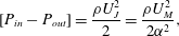
. Applying the Bernoulli theorem along streamlines passing through the hole thus leads to
 $$\begin{eqnarray}[P_{in}-P_{out}]=\frac{\unicode[STIX]{x1D70C}U_{J}^{2}}{2}=\frac{\unicode[STIX]{x1D70C}U_{M}^{2}}{2\unicode[STIX]{x1D6FC}^{2}},\end{eqnarray}$$
that links the pressure jump across the hole and the mean velocity (or flow rate) inside it. Theoretical inviscid calculations by Prandtl and Levi-Civita provided the value
 $\unicode[STIX]{x1D6FC}=0.5$
, that represents also the lower limit for this coefficient. Smith & Walker (Reference Smith and Walker1923), instead, estimated the vena contracta coefficient
 $\unicode[STIX]{x1D6FC}=\unicode[STIX]{x03C0}/(2+\unicode[STIX]{x03C0})\approx 0.611$
for round inviscid jets discharging in open spaces. This value has been found to agree very well with experiments (Cummings & Eversman Reference Cummings and Eversman1983) and numerical calculations (Scarpato, Ducruix & Schuller Reference Scarpato, Ducruix and Schuller2011) at very high Reynolds number.
2.3 Unsteady flow: conductivity and impedance concepts
We now consider the relationship between the pressure jump and the flow rate in the unsteady case, under the hypothesis of harmonic perturbations (2.3). As explained in the introduction, the Rayleigh conductivity (
 $K_{R}$
) is defined as the proportionality coefficient between the acceleration of the fluid particles located within the hole and the pressure jump across the hole. More specifically,
 $$\begin{eqnarray}K_{R}=\frac{-\text{i}\unicode[STIX]{x1D714}\unicode[STIX]{x1D70C}q^{\prime }}{(p_{in}^{\prime }-p_{out}^{\prime })}.\end{eqnarray}$$
The conductivity is, in the general case, a complex quantity, and has the dimension of a length. Following Howe, it is classically noted
 $K_{R}=2R_{h}(\unicode[STIX]{x1D6FE}-\text{i}\unicode[STIX]{x1D6FF})$
. The real part
 $\unicode[STIX]{x1D6FE}$
represents the inertia of the system, while the imaginary part
 $\unicode[STIX]{x1D6FF}$
is directly related to the average value of the power absorbed by the hole. In effect, for harmonic perturbations described with the convention (2.2), the power is given by
 $$\begin{eqnarray}\langle \unicode[STIX]{x1D6F1}\rangle =\langle ([p_{in}^{\prime }-p_{out}^{\prime }]\text{e}^{-\text{i}\unicode[STIX]{x1D714}t}+\text{c.c.})(q^{\prime }\text{e}^{-\text{i}\unicode[STIX]{x1D714}t}+\text{c.c.})\rangle =2\text{Re}([p_{in}^{\prime }-p_{out}^{\prime }]\bar{q^{\prime }}),\end{eqnarray}$$
where the brackets
 $\langle \cdot \rangle$
represent the averaging over a complete period of oscillation
 $2\unicode[STIX]{x03C0}/\unicode[STIX]{x1D714}$
,
 $\text{Re}$
means the real part and the overbar denotes the complex conjugate. Using the definition of the conductivity, this formula directly leads to
 $$\begin{eqnarray}\langle \unicode[STIX]{x1D6F1}\rangle =\frac{4R_{h}\unicode[STIX]{x1D6FF}}{\unicode[STIX]{x1D70C}\unicode[STIX]{x1D714}}|p_{in}^{\prime }-p_{out}^{\prime }|^{2}.\end{eqnarray}$$
So, when
 $\unicode[STIX]{x1D6FF}>0$
, this term represents a resistance (or the ability to absorb acoustic energy), meaning that exciting the jet at a given frequency necessitates the provision of energy by an outer system.
As an alternative to the Rayleigh conductivity, we can also define the impedance of the aperture (
 $Z_{h}$
) as the ratio between the pressure jump and the flow rate:
 $$\begin{eqnarray}Z_{h}=\frac{(p_{in}^{\prime }-p_{out}^{\prime })}{q^{\prime }}\quad \left(=\frac{-\text{i}\unicode[STIX]{x1D714}\unicode[STIX]{x1D70C}}{K_{R}}\right)\!.\end{eqnarray}$$
The impedance is also a complex quantity, with physical dimension
 $\text{Mass}\cdot \text{Length}^{-2}\cdot \text{Time}^{-1}$
. In the following we decompose it as
 $$\begin{eqnarray}Z_{h}=\frac{\unicode[STIX]{x1D70C}U_{M}}{R_{h}^{2}}(Z_{R}+\text{i}Z_{I}),\end{eqnarray}$$
where
 $Z_{R}$
is the dimensionless resistance and
 $Z_{I}$
is the dimensionless reactance. It is easy to verify that the equation (2.6) for the power absorbed by the hole can be written as function of
 $Z_{R}$
as follows:
 $$\begin{eqnarray}\langle \unicode[STIX]{x1D6F1}\rangle =2\frac{\unicode[STIX]{x1D70C}U_{M}}{R_{h}^{2}}Z_{R}|q^{\prime }|^{2}.\end{eqnarray}$$
The Rayleigh conductivity and the impedance are conceptually and practically interchangeable quantities, and both have been used in the literature to characterize the interaction of a jet flow with acoustic fields. In the case of thin holes acting as a sound attenuators, most authors have used the conductivity as initially introduced by Howe. On the other hand, in cases where the jet can act as an energy source for external acoustic systems, leading to instabilities, it proves to be more convenient to employ the impedance (Fabre et al. Reference Fabre, Bonnefis, Charru, Russo, Citro, Giannetti and Luchini2014; Yang & Morgans Reference Yang and Morgans2016). In the present paper, we will use both concepts. A more detailed discussion of impedance-based instability criteria and a parametric study of the impedance of long holes will be given in a forthcoming paper.
2.4 The classical Rayleigh solution in the absence of mean flow
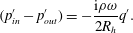
The problem initially solved by Rayleigh (Reference Rayleigh1945) is the simplest situation corresponding to the absence of mean flow. In this case, the problem admits an analytical solution under the framework of potential flow theory. This solution yields a direct proportionality between the flow acceleration and the pressure jump, namely
 $$\begin{eqnarray}(p_{in}^{\prime }-p_{out}^{\prime })=-\frac{\text{i}\unicode[STIX]{x1D70C}\unicode[STIX]{x1D714}}{2R_{h}}q^{\prime }.\end{eqnarray}$$
The classical interpretation of this result is that the fluid in the vicinity of the hole behaves as a simple solid plug with mass
 $m=\unicode[STIX]{x1D70C}\unicode[STIX]{x03C0}R_{h}^{2}\ell _{eff}$
oscillating across the hole, where
 $\ell _{eff}$
is the equivalent length of the plug given by
 $\ell _{eff}=\unicode[STIX]{x03C0}R_{h}/2$
.
When reformulated in terms of conductivity (respectively impedance) and using the non-dimensionalization choices introduced in the previous section, the Rayleigh solution thus corresponds to
 $\unicode[STIX]{x1D6FE}=1;\unicode[STIX]{x1D6FF}=0$
(respectively
 $Z_{R}=0;Z_{I}=-\text{i}\unicode[STIX]{x1D6FA}/2$
). An obvious consequence is that, under this model, the power absorbed by the hole predicted by (2.10) is exactly zero.
2.5 Review and criticism of Howe’s inviscid model
We now review and discuss in more detail the classical model of Howe already mentioned in the introduction. Howe models the jet as a cylindrical vortex sheet of constant radius
 $R_{h}$
formed at the rim of the aperture. He subsequently assumes a vorticity perturbation of this vortex sheet with the form
 $$\begin{eqnarray}\unicode[STIX]{x1D709}^{\prime }=\unicode[STIX]{x1D70E}H(x)\unicode[STIX]{x1D6FF}(r-R_{h})\exp [-\text{i}\unicode[STIX]{x1D714}(t-x/U_{c})],\end{eqnarray}$$
where
 $\unicode[STIX]{x1D6FF}$
and
 $H$
are respectively the Dirac and Heaviside functions,
 $U_{c}$
the assumed convection velocity of vorticity structures and
 $\unicode[STIX]{x1D70E}$
the amplitude of the vorticity perturbation. This later parameter is determined by imposing a Kutta condition (Crighton Reference Crighton1985), requiring finite velocity and pressure fluctuations at the rim of the hole. Starting from this point, and going through a series of very technical mathematical transformations, Howe was eventually able to predict the Rayleigh conductivity under the following analytical form:
 $$\begin{eqnarray}K_{R}=2R_{h}(\unicode[STIX]{x1D6FE}-\text{i}\unicode[STIX]{x1D6FF})=2R_{h}\left\{1+\frac{(\unicode[STIX]{x03C0}/2)I_{1}(\unicode[STIX]{x1D6FA}^{H})\text{e}^{-\unicode[STIX]{x1D6FA}^{H}}-\text{i}K_{1}(\unicode[STIX]{x1D6FA}^{H})\sinh (\unicode[STIX]{x1D6FA}^{H})}{\unicode[STIX]{x1D6FA}^{H}[(\unicode[STIX]{x03C0}/2)I_{1}(\unicode[STIX]{x1D6FA}^{H})\text{e}^{-\unicode[STIX]{x1D6FA}^{H}}+\text{i}K_{1}(\unicode[STIX]{x1D6FA}^{H})\cosh (\unicode[STIX]{x1D6FA}^{H})]}\right\}\!,\end{eqnarray}$$
where
 $I_{1}$
and
 $K_{1}$
are the order-one modified Bessel functions of respectively first and second kind and
 $\unicode[STIX]{x1D6FA}^{H}=\unicode[STIX]{x1D714}R_{h}/U_{c}$
is the Strouhal number.
Despite its mathematical rigor, a number of starting hypotheses of Howe’s model are questionable. The main caveats of the model can be summarized in four points:
(i) First, the study models the mean flow as a cylindrical vortex sheet with radius
$R_{h}$
, and constant velocity
$U_{M}$
, hence completely overlooks the vena contracta phenomenon discussed above. In a subsequent step of his analysis (p. 215 of his paper), Howe intended to incorporate partially this effect in his model, but this a posteriori modification remains imperfect.(ii) Secondly, Howe’s model assumes that the perturbation affects only the strength of the vortex sheet but not its location, so that the perturbed vortex sheet is assumed to remain perfectly cylindrical. A better starting point would be to assume a vortex sheet with location given by (see figure 1):
(2.14)where$$\begin{eqnarray}r_{J}(r)=R_{J}+\unicode[STIX]{x1D700}\unicode[STIX]{x1D702}(x,r,t)=R_{J}+\unicode[STIX]{x1D700}\unicode[STIX]{x1D702}^{\prime }(r)\exp [\text{i}k(\unicode[STIX]{x1D714})x-\text{i}\unicode[STIX]{x1D714}t],\end{eqnarray}$$
$k(\unicode[STIX]{x1D714})=k_{r}+\text{i}k_{i}$
is a complex wavenumber which has to be determined as a function of the frequency
$\unicode[STIX]{x1D714}$
. The inviscid stability analysis of this model is a classical problem whose solution can be found, for instance, in Batchelor & Gill (Reference Batchelor and Gill1962) or in Abid, Brachet & Huerre (Reference Abid, Brachet and Huerre1993). For completeness, this problem is reviewed in appendix A.(iii) Thirdly, the starting point of Howe’s analysis (2.12) assumes that the perturbations are convected at a constant velocity
$U_{c}$
which is assumed to be half the velocity of the jet. This choice is justified by analogy with the classical result for the Kelvin–Helmholtz instability of a planar vortex sheet. This choice is a questionable simplification and it would seem more rigorous to predict
$U_{c}$
using spatial stability analysis of the cylindrical vortex sheet model, namely
$U_{c}=k_{r}/\unicode[STIX]{x1D714}$
. This analysis shows that for small frequencies the convection velocity is actually closer to the velocity of the jet than half its value (see appendix A).(iv) Finally, Howe completely ignores the fact that perturbations of the vortex sheet are spatially amplified in addition to being convected.





According to the two last criticisms, it would thus seem more appropriate to replace the starting point (2.12) by the following ansatz:
 $$\begin{eqnarray}\unicode[STIX]{x1D709}^{\prime }=\unicode[STIX]{x1D70E}H(x)\unicode[STIX]{x1D6FF}(r_{J}(r)-R_{J}-\unicode[STIX]{x1D700}\unicode[STIX]{x1D702}^{\prime }(r)\exp [\text{i}k(\unicode[STIX]{x1D714})x-\text{i}\unicode[STIX]{x1D714}t])\exp [\text{i}k(\unicode[STIX]{x1D714})x-\text{i}\unicode[STIX]{x1D714}t].\end{eqnarray}$$
We have not intended to reconstruct the whole analysis from this modified starting point, an option which would anyway not address the first criticism discussed above (vena contracta effect) and would remain limited to the high Reynolds number range. Instead, our chosen approach to address the problem is to compute the impedance (or alternatively the conductivity) through a global resolution of the linearized Navier–Stokes equations (LNSE) for given values of the Reynolds number.
3 The viscous problem: analysis and numerical method for the linear approach
3.1 General equations
Taking the diameter of the hole
 $D_{h}=2R_{h}$
as a length scale and the mean velocity
 $U_{M}$
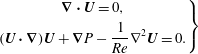
as a velocity scale, the problem is governed by the axial–symmetric incompressible dimensionless Navier–Stokes equations:
 $$\begin{eqnarray}\left.\begin{array}{@{}c@{}}\displaystyle \unicode[STIX]{x1D735}\boldsymbol{\cdot }\boldsymbol{u}=0,\\ \displaystyle \unicode[STIX]{x2202}_{t}\boldsymbol{u}+(\boldsymbol{u}\boldsymbol{\cdot }\unicode[STIX]{x1D735})\boldsymbol{u}+\unicode[STIX]{x1D735}p-\displaystyle \frac{1}{Re}\unicode[STIX]{x1D6FB}^{2}\boldsymbol{u}=0,\end{array}\right\}\end{eqnarray}$$
where
 $\boldsymbol{u}(x,r,t)=(u_{x},u_{r})$
and
 $p$
is the reduced pressure. The variables
 $x$
and
 $r$
are respectively the axial and radial coordinate while
 $u_{x}$
and
 $u_{r}$
represent the axial and radial velocity components.
The flow is further decomposed into a base flow
 $(\boldsymbol{U},P)$
associated with the mean flux
 $Q$
and a harmonic perturbation
 $\unicode[STIX]{x1D700}(\boldsymbol{u}^{\prime },p^{\prime })\text{e}^{-\text{i}\unicode[STIX]{x1D714}t}$
associated with the oscillating flow rate
 $q^{\prime }\text{e}^{-\text{i}\unicode[STIX]{x1D714}t}$
. A crucial hypothesis in this treatment is that the amplitude of the harmonic perturbation is small, namely
 $\unicode[STIX]{x1D700}\ll 1$
. Inserting this decomposition into the Navier–Stokes equations (3.1) and linearizing, two different sets of partial differential equations are obtained:
(i) First, the leading order yields the base-flow equations:
(3.2)The link between the base flow$$\begin{eqnarray}\left.\begin{array}{@{}c@{}}\displaystyle \unicode[STIX]{x1D735}\boldsymbol{\cdot }\boldsymbol{U}=0,\\ \displaystyle (\boldsymbol{U}\boldsymbol{\cdot }\unicode[STIX]{x1D735})\boldsymbol{U}+\unicode[STIX]{x1D735}P-\frac{1}{Re}\unicode[STIX]{x1D6FB}^{2}\boldsymbol{U}=0.\end{array}\right\}\end{eqnarray}$$
$(\boldsymbol{U},P)$
and the quantities
$P_{in}$
,
$P_{out}$
,
$Q$
introduced in § 2 is given by the asymptotic matching conditions and flow rate definition as follows: (3.3)$$\begin{eqnarray}\displaystyle & \displaystyle P(x,r)\rightarrow P_{in}\quad \text{for }\sqrt{x^{2}+r^{2}}\rightarrow \infty \text{and }x<0, & \displaystyle\end{eqnarray}$$
(3.4)$$\begin{eqnarray}\displaystyle & \displaystyle P(x,r)\rightarrow P_{out}\quad \text{for }\sqrt{x^{2}+r^{2}}\rightarrow \infty \text{and }x>0, & \displaystyle\end{eqnarray}$$
(3.5)where$$\begin{eqnarray}\displaystyle & \displaystyle \int _{{\mathcal{S}}}\boldsymbol{U}\boldsymbol{\cdot }\boldsymbol{n}\,\text{d}S=Q, & \displaystyle\end{eqnarray}$$
${\mathcal{S}}$
is any surface traversed by the flow and
$\boldsymbol{n}$
a normal unitary vector oriented in the direction of the flow.(ii) Secondly, the
$\unicode[STIX]{x1D700}$
-order yields the linearized Navier–Stokes equations (LNSE) governing the perturbation: (3.6)The link with the quantities$$\begin{eqnarray}\left.\begin{array}{@{}c@{}}\displaystyle \unicode[STIX]{x1D735}\boldsymbol{\cdot }\boldsymbol{u}^{\prime }=0,\\ \displaystyle -\text{i}\unicode[STIX]{x1D714}\boldsymbol{u}^{\prime }+(\boldsymbol{U}\boldsymbol{\cdot }\unicode[STIX]{x1D735})\boldsymbol{u}^{\prime }+(\boldsymbol{u}^{\prime }\boldsymbol{\cdot }\unicode[STIX]{x1D735})\boldsymbol{U}+\unicode[STIX]{x1D735}p^{\prime }-\frac{1}{Re}\unicode[STIX]{x1D6FB}^{2}\boldsymbol{u}^{\prime }=0.\end{array}\right\}\end{eqnarray}$$
$p_{in}^{\prime }$
,
$p_{out}^{\prime }$
,
$q^{\prime }$
introduced in § 2 and allowing to define the impedance/conductivity is: (3.7)$$\begin{eqnarray}\displaystyle & \displaystyle p^{\prime }(x,r)\rightarrow p_{in}^{\prime }\quad \text{for }\sqrt{x^{2}+r^{2}}\rightarrow \infty \text{and }x<0, & \displaystyle\end{eqnarray}$$
(3.8)$$\begin{eqnarray}\displaystyle & \displaystyle p^{\prime }(x,r)\rightarrow p_{out}^{\prime }\quad \text{for }\sqrt{x^{2}+r^{2}}\rightarrow \infty \text{and }x>0, & \displaystyle\end{eqnarray}$$
(3.9)$$\begin{eqnarray}\displaystyle & \displaystyle \int _{{\mathcal{S}}}\boldsymbol{u}^{\prime }\boldsymbol{\cdot }\boldsymbol{n}\,\text{d}S=q^{\prime }. & \displaystyle\end{eqnarray}$$











Note that, as is customary when dealing with incompressible flows, the pressure is defined up to an arbitrary constant. We can choose this constant by setting
 $P_{out}=0$
and
 $p_{out}^{\prime }=0$
in (3.4) and (3.8), so that the mean pressure drop and fluctuating pressure drop are actually given by
 $[P_{in}-P_{out}]=P_{in}$
,
 $[p_{in}^{\prime }-p_{out}^{\prime }]=p_{in}^{\prime }$
.
With the addition of no-slip conditions
 $\boldsymbol{U}=\boldsymbol{u}^{\prime }=\mathbf{0}$
on the upstream and downstream surfaces of the plate (noted
 $\unicode[STIX]{x1D6E4}_{w}$
) and symmetry conditions
 $U_{r}=u_{r}^{\prime }=0$
;
 $\unicode[STIX]{x2202}U_{x}/\unicode[STIX]{x2202}r=\unicode[STIX]{x2202}u_{x}^{\prime }/\unicode[STIX]{x2202}r=0$
at the axis (noted
 $\unicode[STIX]{x1D6E4}_{axis}$
), the set of (3.2)–(3.9) completely defines the nonlinear problem allowing us to compute the vena contracta coefficient
 $\unicode[STIX]{x1D6FC}$
and the linear problem allowing us to compute the impedance/conductivity.
In practice, the boundary conditions at
 $\sqrt{x^{2}+r^{2}}$
have to be imposed at the boundaries of a finite computational domain, both upstream and downstream. Treatment of these boundary conditions requires special attention and is detailed in the next sections.
Structure of the mesh
 $M_{1}$
obtained at the end of the mesh adaptation process, and nomenclature of boundaries. The mesh is adapted to both the base flow for
 $Re=1000$
and the harmonic perturbation for
 $\unicode[STIX]{x1D714}=2$
. The inset shows a zoom of the mesh structure in the range
 $X\in [-0.5;0.8]R_{h}$
and
 $R\in [0.5;1.3]R_{h}$
. Note that owing to the coordinate mapping, the actual dimension of the outlet domain is
 $[x_{max},r_{max}]=[1022+306i,337]$
.
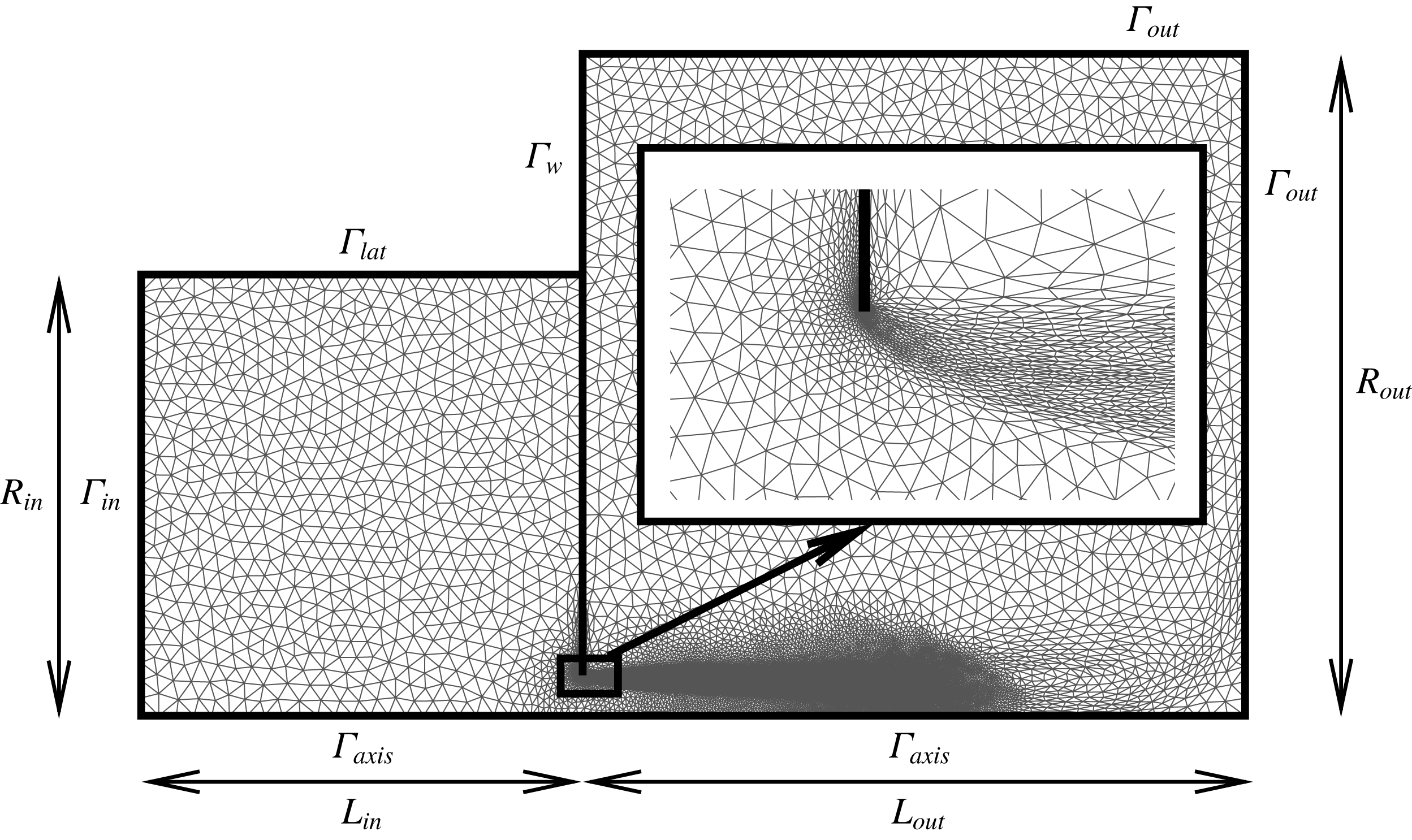
3.2 Upstream domain
As sketched in figure 1, the upstream domain is expected to originate from an upstream container of large dimension, and sufficiently far away from the hole. Moreover, the flow is assumed to be radially convergent. However, in the numerical implementation, it is necessary to specify a given geometry for this upstream domain. Here, we chose to assume that the upstream region is a closed cavity of cylindrical section, with radius
 $R_{in}$
and length
 $L_{in}$
. The volumetric flux conditions (3.5) and (3.9) are imposed by assuming that both the base flow and the perturbation velocities are constant along the bottom of the cavity, noted
 $\unicode[STIX]{x1D6E4}_{in}$
(see figure 2), i.e.
 $$\begin{eqnarray}\left.\begin{array}{@{}c@{}}\boldsymbol{U}=Q/S_{in}\boldsymbol{n}\\ \boldsymbol{u}^{\prime }=q^{\prime }/S_{in}\boldsymbol{n}\end{array}\right\}\quad \text{on }\unicode[STIX]{x1D6E4}_{in},\end{eqnarray}$$
where
 $S_{in}=\unicode[STIX]{x03C0}R_{in}^{2}$
is the area of the bottom wall. The values of
 $Q$
and
 $q^{\prime }$
have been selected in order to have a mean velocity equal to one into the hole, for both the base flow and the perturbation. The pressure levels
 $P_{in}$
and
 $p_{in}^{\prime }$
, which are required for the calculation of the mean pressure loss (and the vena contracta coefficient) and the impedance (or conductivity), are extracted by averaging along the inlet boundary:
 $$\begin{eqnarray}\left.\begin{array}{@{}c@{}}\displaystyle P_{in}=2\unicode[STIX]{x03C0}/S_{in}\int _{0}^{R_{in}}P(r)r\,\text{d}r\\ \displaystyle {p^{\prime }}_{in}=2\unicode[STIX]{x03C0}/S_{in}\int _{0}^{R_{in}}p^{\prime }(r)r\,\text{d}r\end{array}\right\}\quad \text{on }\unicode[STIX]{x1D6E4}_{in}.\end{eqnarray}$$
Since the upstream cavity used in our mesh definition is expected to represent an upper domain of infinite extend, its precise geometry has no real importance, but is dimension has to be large enough so that the results are independent of this geometry. In practice we verified that the choice
 $L_{in}=R_{in}=10R_{h}$
fulfils this condition. Finally, at the lateral wall of the cavity for
 $r=R_{in}$
(noted
 $\unicode[STIX]{x1D6E4}_{lat}$
), we simply choose no-penetration (
 $u_{r}=0$
) and no-stress (
 $\unicode[STIX]{x2202}_{r}u_{x}=0$
) conditions for both base flow and perturbation. This condition ensures that the volumetric flux imposed at the bottom of the cavity effectively corresponds to the one traversing the hole, preventing the occurrence of an unphysical boundary layer that would be obtained using a no-slip condition.
3.3 Downstream domain: boundary conditions and change of coordinates
The treatment of the outlet boundary conditions is a delicate point here, as the structure of the perturbation leads to some difficulties, especially when the Reynolds number becomes large. In effect, due to the strongly spatially unstable nature of the jet, all perturbations are strongly amplified along the axial direction. In particular, the pressure field
 $p^{\prime }(x,r)$
can be reach huge levels (reaching
 $10^{15}$
or even more for
 $Re\approx 3000$
) along the axis (
 $r=0$
) for large
 $x$
, and this conflicts with the necessity of imposing the boundary condition
 $p_{out}^{\prime }=0$
at a finite distance
 $x_{max}$
corresponding to the boundary of the computational domain.
To detail the origin of the problem and introduce the idea used to overcome it, let us review the classical modelling of the Kelvin–Helmholtz instability for a planar shear layer of zero thickness in the inviscid case. The formal derivation can be found in any classical textbook on hydrodynamical stability (see for example Drazin & Reid (Reference Drazin and Reid2004) or Charru (Reference Charru2011)). Consider as base flow a shear layer separating two regions of constant axial velocity, namely
 $u_{x}=U$
for
 $r<0$
and
 $u_{x}=0$
for
 $r>0$
. Now assume that the perturbation consists of a displacement of the shear layer with the form
 $$\begin{eqnarray}\unicode[STIX]{x1D702}(x,r,t)\propto \text{e}^{\text{i}kx-\text{i}\unicode[STIX]{x1D714}t},\end{eqnarray}$$
and assume a similar modal expansion for the velocity potential in the upper and lower regions. Matching the two regions at the interface leads to the classical dispersion relation:
 $$\begin{eqnarray}c\equiv \frac{\unicode[STIX]{x1D714}}{k}=\frac{1\pm \text{i}}{2}U.\end{eqnarray}$$
In a temporal stability framework, this means that a perturbation with a real wavenumber
 $k$
is convected downstream with a phase velocity
 $U/2$
and temporally amplified with a growth rate
 $Uk/2$
. On the other hand, in a spatial stability framework which is more relevant here, a perturbation with real frequency
 $\unicode[STIX]{x1D714}$
will be spatially amplified downstream with a complex wavenumber
 $k$
and will diverge at
 $x\rightarrow +\infty$
. This divergence forbids a global resolution of the function
 $\unicode[STIX]{x1D702}(x,t)$
when the variable
 $x$
is real. However, the problem disappears if we consider an analytical continuation of the function
 $\unicode[STIX]{x1D702}(x,t)$
with a complex variable
 $x$
. More specifically, as
 $\arg (k)=-\unicode[STIX]{x03C0}/4$
, the function
 $\unicode[STIX]{x1D702}(x,t)$
becomes convergent as soon as
 $|x|\rightarrow \infty$
in a direction of the complex plane verifying
 $\unicode[STIX]{x03C0}/4<\arg (x)<5\unicode[STIX]{x03C0}/4$
. These considerations suggest a possible way to overcome the problem, namely using a complex coordinate change
 $x={\mathcal{G}}_{x}(X)$
which maps a (real) numerical coordinate
 $X$
defined over a finite-size computational downstream domain
 $X\in [-L_{in};L_{out}]$
, onto the physical coordinate
 $x$
in such a way that it enters the complex plane and follows a direction where the perturbation is spatially damped.
The coordinate mapping effectively transforms the outlet location
 $X=L_{out}$
into a location
 $x=x_{max}={\mathcal{G}}_{x}(L_{out})$
located in the complex plane. In order for the boundary conditions at the outlet
 $X=L_{out}$
of the computational domain to best represent the physical boundary condition at
 $|x|\rightarrow \infty$
, it is desirable for
 $x_{max}={\mathcal{G}}_{x}(L_{out})$
to be as large as possible. This can be achieved using coordinate stretching in order to have short numerical domains and large physical ones.
Combining both ideas, namely stretching and complex mapping, we designed the following mapping function from numerical coordinate
 $X$
to physical coordinate
 $x$
:
 $$\begin{eqnarray}\displaystyle x={\mathcal{G}}_{x}(X) & = & \displaystyle \frac{X}{\displaystyle \left[1-\left(\frac{X}{L_{A}}\right)^{2}\right]^{2}}\left[1+\text{i}\unicode[STIX]{x1D6FE}_{c}\tanh \left(\frac{X}{2L_{C}}\right)^{2}\right]\quad \text{for }X>0,\nonumber\\ \displaystyle & = & \displaystyle X\quad \text{for }X<0.\end{eqnarray}$$
This function is characterized by three parameters which have the following interpretation. First, the parameter
 $L_{C}$
controls the transition range from real coordinate to complex coordinate. For
 $X\ll L_{C}$
the mapping is almost identity
 $({\mathcal{G}}_{x}(X)\approx X)$
so that the transition with the upstream, unmapped domain is as smooth as possible. For
 $X\approx L_{c}$
the imaginary part of the corresponding physical coordinate
 $x$
gradually increases. For
 $X\gg L_{c}$
the argument of
 $x$
asymptotes to a constant value, namely
 $\arg (x)\approx \tan ^{-1}(\unicode[STIX]{x1D6FE}_{c})$
. The third parameter
 $L_{A}$
controls the stretching effect associated with the coordinate mapping. This parameter has to be chosen so that
 $L_{A}>L_{out}$
.
 $L_{A}\rightarrow \infty$
means no coordinate stretching, so that the real part of
 $x_{max}$
is the same as the dimension
 $L_{out}$
of the computational domain, while if
 $L_{A}-L_{out}$
is small the corresponding
 $x_{max}$
is rejected very far away in the complex plane.
Finally, although the issue is less crucial with respect to the axial coordinate, we also used a mapping
 $r={\mathcal{G}}_{r}(R)$
to stretch the radial coordinate from
 $R\in [0,R_{out}]$
to
 $r\in [0,r_{out}]$
in order to enlarge the effective radial dimension of the physical domain. Here there is no point in using a complex deformation, so we used the following mapping function:
 $$\begin{eqnarray}\displaystyle r={\mathcal{G}}_{r}(R) & = & \displaystyle R_{M}+\frac{R-R_{M}}{\displaystyle \left[1-\left(\frac{R-R_{M}}{R_{A}-R_{M}}\right)^{2}\right]^{2}}\quad \text{for }X>0\text{ and }R>R_{A},\nonumber\\ \displaystyle & = & \displaystyle R\quad \text{otherwise}.\end{eqnarray}$$
This function leaves the radial coordinate unchanged in the region
 $r<R_{M}$
where the jet develops, but it stretches the limit of the domain from
 $R_{out}$
to
 $r_{out}={\mathcal{G}}_{r}(R_{out})$
which is very large as soon as
 $R_{A}$
is close to
 $R_{out}$
(with the constraint
 $R_{A}>R_{out}$
).
Having explained this change of coordinates, it remains to specify the numerical boundary conditions effectively used at the boundaries of the numerical domain
 $R=R_{out}$
(corresponding to
 $r=r_{out}$
) and
 $X=L_{out}$
(corresponding to
 $x=x_{max}$
). In the framework of finite elements, the usual way to impose outlet conditions is to take advantage of integration by parts leading to the weak formulation. The most natural condition emerging in this way is the zero-traction condition, namely
 $-p\boldsymbol{n}+Re^{-1}\unicode[STIX]{x1D735}\boldsymbol{u}\boldsymbol{\cdot }\boldsymbol{n}=0$
. In the present case, we used the zero-traction condition as an approximation of the physical condition
 $p=0$
for both the base-flow and perturbation computations. This choice is justified if the viscous stresses are negligible in the vicinity of the boundaries of the domain, which turns out to be the case here.
We stress that using the present method, outflow boundary conditions are effectively applied at a location
 $x_{max}$
located in the complex plane. The validity of the method is not justified by rigorous mathematical argument, but only by the fact that it effectively works. Detailed validations are given in § B.1 of this paper. In particular, we show that at low Reynolds numbers results obtained with and without complex mapping are identical, and are independent of the precise choice of the parameters (
 $\unicode[STIX]{x1D6FE}_{c},L_{C},L_{A}$
) for the mapping function.
Note that the idea of using a complex coordinate mapping is not completely new. Indeed, the method is conceptually similar to the perfectly matching layer (PML) method, which is a numerical approach largely used in electromagnetics and acoustics to impose non-reflection boundary conditions in wave propagation problems (see Colonius (Reference Colonius2004) for a complete review). In stability studies of incompressible flows, complex coordinate mappings have also been used in linear problems involving a single spatial coordinate and characterized by a critical layer singularity (see for instance Fabre, Sipp & Jacquin Reference Fabre, Sipp and Jacquin2006) and mathematical theorems are available to justify how to choose the mapping as a function of the singularities of the problem (see for example Bender & Orszag (Reference Bender and Orszag2013)). However, we are not aware of any usage of such methods to get rid of convective amplifications (which is a different issue compared to reflexion of waves along boundaries and critical layer singularities). The usage of complex mappings for solving a nonlinear problem (i.e. computation of the base flow) involving two spatial coordinates is also totally new to our knowledge.
3.4 Numerical implementation
The numerical resolution of the problem was performed with a finite element method, using the FreeFem++ (http://www.freefem.org) open source code (Hecht (Reference Hecht2012)). The procedure follows the classical approach initially introduced by Sipp & Lebedev (Reference Sipp and Lebedev2007). The only notable originalities are the introduction of the complex mapping into the weak formulation, and the use of mesh adaptation using the adaptmesh command provided by the Freefem++ (see Fabre et al. Reference Fabre, Sabino, Citro, Bonnefis and Giannetti2018 for a demonstration of the efficiency of this method for solving linear and nonlinear problems arising from stability analysis).
In order to solve the problem, the base flow and perturbation equations have first to be expressed in terms of the mapped coordinates. The treatment of both sets of equations in very similar so we document only the base-flow equations. First, the spatial derivatives have to be modified as follows:
 $$\begin{eqnarray}\left.\begin{array}{@{}c@{}}\displaystyle \unicode[STIX]{x2202}_{x}\equiv {\mathcal{H}}_{x}(X)\unicode[STIX]{x2202}_{X}\quad \text{with }{\mathcal{H}}_{x}=\frac{1}{\unicode[STIX]{x2202}_{X}{\mathcal{G}}_{x}(X)},\\ \displaystyle \unicode[STIX]{x2202}_{r}\equiv {\mathcal{H}}_{r}(R)\unicode[STIX]{x2202}_{R}\quad \text{with }{\mathcal{H}}_{r}=\frac{1}{\unicode[STIX]{x2202}_{R}{\mathcal{G}}_{r}(R)}.\end{array}\right\}\end{eqnarray}$$
The steady incompressible Navier–Stokes equations (3.2) thus take the following form:
 $$\begin{eqnarray}\left.\begin{array}{@{}c@{}}\displaystyle {\mathcal{H}}_{x}\unicode[STIX]{x2202}_{X}U_{x}+{\mathcal{H}}_{r}/r\unicode[STIX]{x2202}_{R}(rU_{r})=0,\\ \displaystyle \mathscr{C}\{U_{x}\}+{\mathcal{H}}_{x}\unicode[STIX]{x2202}_{X}P-\frac{1}{Re}[{\mathcal{H}}_{x}\unicode[STIX]{x2202}_{X}({\mathcal{H}}_{x}\unicode[STIX]{x2202}_{X}U_{x})+{\mathcal{H}}_{r}/r\unicode[STIX]{x2202}_{R}(r{\mathcal{H}}_{r}\unicode[STIX]{x2202}_{r}U_{x})]=0,\\ \displaystyle \mathscr{C}\{U_{r}\}+{\mathcal{H}}_{r}\unicode[STIX]{x2202}_{R}P-\frac{1}{Re}[{\mathcal{H}}_{x}\unicode[STIX]{x2202}_{X}({\mathcal{H}}_{x}\unicode[STIX]{x2202}_{X}U_{r})-U_{r}/r^{2}+{\mathcal{H}}_{r}/r\unicode[STIX]{x2202}_{R}(r{\mathcal{H}}_{r}\unicode[STIX]{x2202}_{r}U_{r})]=0,\end{array}\right\}\end{eqnarray}$$
where, from (3.15),
 $r={\mathcal{G}}_{r}(R)$
and
 $\mathscr{C}\{\cdot \}=U_{x}{\mathcal{H}}_{x}\unicode[STIX]{x2202}_{X}(\cdot )+U_{r}{\mathcal{H}}_{r}\unicode[STIX]{x2202}_{R}(\cdot )$
. The weak formulation is classically obtained by multiplying by test functions
 $[U_{x}^{+},U_{r}^{+},P^{+}]$
and integrating over the domain. Note that this integration has to be done over the physical domain, so in terms of the numerical variables the elementary volume of integration is
 $\text{d}V=2\unicode[STIX]{x03C0}r\,\text{d}r\,\text{d}x=2\unicode[STIX]{x03C0}({\mathcal{H}}_{x}{\mathcal{H}}_{r})^{-1}r\,\text{d}R\,\text{d}X\equiv 2\unicode[STIX]{x03C0}({\mathcal{H}}_{x}{\mathcal{H}}_{r})^{-1}{\mathcal{G}}_{r}(R)\,\text{d}R\,\text{d}X$
. After integration by parts of the pressure gradient and Laplacian terms of equation (3.17), we are thus lead to the following weak formulation of the mapped Navier–Stokes equations:
 $$\begin{eqnarray}\displaystyle & & \displaystyle -\int [U_{x}^{+}(U_{x}{\mathcal{H}}_{x}\unicode[STIX]{x2202}_{X}U_{x}+U_{r}{\mathcal{H}}_{r}\unicode[STIX]{x2202}_{R}U_{x})+U_{r}^{+}(U_{x}{\mathcal{H}}_{x}\unicode[STIX]{x2202}_{X}U_{r}+U_{r}{\mathcal{H}}_{r}\unicode[STIX]{x2202}_{R}U_{r})]\,\text{d}V\nonumber\\ \displaystyle & & \displaystyle \qquad +\,\int [P({\mathcal{H}}_{x}\unicode[STIX]{x2202}_{X}U_{x}^{+}+{\mathcal{H}}_{r}\unicode[STIX]{x2202}_{R}U_{r}^{+}+U_{r}^{+}/r)-P^{+}({\mathcal{H}}_{x}\unicode[STIX]{x2202}_{X}U_{x}+{\mathcal{H}}_{r}\unicode[STIX]{x2202}_{R}U_{r}+U_{r}/r)]\,\text{d}V\nonumber\\ \displaystyle & & \displaystyle \qquad -\,\frac{1}{Re}\int [{\mathcal{H}}_{x}^{2}\unicode[STIX]{x2202}_{X}U_{x}\unicode[STIX]{x2202}_{X}U_{x}^{+}+{\mathcal{H}}_{r}^{2}\unicode[STIX]{x2202}_{R}U_{x}\unicode[STIX]{x2202}_{R}U_{x}^{+}]\,\text{d}V\nonumber\\ \displaystyle & & \displaystyle \qquad -\,\frac{1}{Re}\int [{\mathcal{H}}_{x}^{2}\unicode[STIX]{x2202}_{X}U_{r}\unicode[STIX]{x2202}_{X}U_{r}^{+}+{\mathcal{H}}_{r}^{2}\unicode[STIX]{x2202}_{R}U_{r}\unicode[STIX]{x2202}_{R}U_{r}^{+}+U_{r}U_{r}^{+}/r^{2}]\,\text{d}V\nonumber\\ \displaystyle & & \displaystyle \quad =0.\end{eqnarray}$$
Note that with this formulation, the no-traction boundary conditions at the outlet boundary, as well as the symmetry condition at the axis and the zero tangential stress condition at the lateral wall of the cavity are automatically satisfied thanks to the integration by parts. The other boundary conditions are imposed by penalization.
The LNSE (3.6) is treated in a similar way, leading to the following weak formulation:
 $$\begin{eqnarray}\displaystyle & & \displaystyle \text{i}\unicode[STIX]{x1D714}\int [U_{x}^{+}u_{x}^{\prime }+U_{r}u_{r}^{\prime }]\,\text{d}V\nonumber\\ \displaystyle & & \displaystyle \qquad +\,\int [U_{x}^{+}(U_{x}{\mathcal{H}}_{x}\unicode[STIX]{x2202}_{X}u_{x}^{\prime }+u_{x}^{\prime }{\mathcal{H}}_{x}\unicode[STIX]{x2202}_{X}U_{x}+u_{r}^{\prime }{\mathcal{H}}_{r}\unicode[STIX]{x2202}_{R}U_{x}+U_{r}{\mathcal{H}}_{r}\unicode[STIX]{x2202}_{R}u_{x}^{\prime })]\,\text{d}V\nonumber\\ \displaystyle & & \displaystyle \qquad +\,\int [+U_{r}^{+}(U_{x}{\mathcal{H}}_{x}\unicode[STIX]{x2202}_{X}u_{r}+u_{x}^{\prime }{\mathcal{H}}_{x}\unicode[STIX]{x2202}_{X}U_{r}+u_{r}^{\prime }{\mathcal{H}}_{r}\unicode[STIX]{x2202}_{R}U_{r}+U_{r}{\mathcal{H}}_{r}\unicode[STIX]{x2202}_{R}u_{r}^{\prime })]\,\text{d}V\nonumber\\ \displaystyle & & \displaystyle \qquad -\,\int [p^{\prime }({\mathcal{H}}_{x}\unicode[STIX]{x2202}_{X}U_{x}^{+}+{\mathcal{H}}_{r}\unicode[STIX]{x2202}_{R}U_{r}^{+}+U_{r}^{+}/r)+P^{+}({\mathcal{H}}_{x}\unicode[STIX]{x2202}_{X}u_{x}^{\prime }+{\mathcal{H}}_{r}\unicode[STIX]{x2202}_{R}u_{r}^{\prime }+u_{r}^{\prime }/r)]\,\text{d}V\nonumber\\ \displaystyle & & \displaystyle \qquad +\,\frac{1}{Re}\int [{\mathcal{H}}_{x}^{2}\unicode[STIX]{x2202}_{X}u_{x}^{\prime }\unicode[STIX]{x2202}_{X}U_{x}^{+}+{\mathcal{H}}_{r}^{2}\unicode[STIX]{x2202}_{R}u_{x}^{\prime }\unicode[STIX]{x2202}_{R}U_{x}^{+}]\,\text{d}V\nonumber\\ \displaystyle & & \displaystyle \qquad +\,\frac{1}{Re}\int [{\mathcal{H}}_{x}^{2}\unicode[STIX]{x2202}_{X}u_{r}^{\prime }\unicode[STIX]{x2202}_{X}U_{r}^{+}+{\mathcal{H}}_{r}^{2}\unicode[STIX]{x2202}_{R}u_{r}^{\prime }\unicode[STIX]{x2202}_{R}U_{r}^{+}+u_{r}^{\prime }U_{r}^{+}/r^{2}]\,\text{d}V\nonumber\\ \displaystyle & & \displaystyle \quad =0.\end{eqnarray}$$
Once the weak formulation is written, the discrete matrices are assembled using classical Taylor–Hood
 $(P_{2},P_{2},P_{1})$
finite elements for the spatial discretization. The use of mesh adaptation to generate a efficient mesh is done in a way very similar to that explained in Fabre et al. (Reference Fabre, Sabino, Citro, Bonnefis and Giannetti2018). The procedure is as follows:
(i) we generate an initial coarse mesh using the Delaunay–Voronoi triangulation of the domain;
(ii) we use Newton iteration to compute a base flow at a moderate value of the Reynolds (for instance
$Re=10$
);(iii) we adapt the mesh to the base-flow solution of the previous step and recompute the base flow on the resulting mesh;
(iv) we repeat points (ii) and (iii) for gradually increasing values the Reynolds number up
$Re=1000$
.After this stage, we are guaranteed to have a mesh yielding converged results for base-flow characteristics;
(v) we solve the linear problem for a value of
$\unicode[STIX]{x1D714}$
in the range of interest, adapt the mesh to fit with the corresponding structure and recompute the base flow on the resulting mesh.


After this stage, we are ensured to have a mesh yielding converged results for both the base flow and the perturbation for a given
 $\unicode[STIX]{x1D714}$
. For even better efficiency, it is also possible to do the last mesh adaptation
 $(v)$
for two values of
 $\unicode[STIX]{x1D714}$
spanning the range of parameters in which converged results are expected.
To obtain the results presented in the next sections, two different meshes were designed in this way. The first mesh, noted
 $\mathbb{M}_{0}$
, is generated without the use of complex mapping, with a large domain corresponding to
 $L_{out}=x_{max}=80$
. This mesh was used to compute impedances at low Reynolds number (up to 1000) and to plot the base-flow characteristics. The second, noted
 $\mathbb{M}_{1}$
, uses complex mapping and was used for most results at larger Reynolds number values. The structure of this mesh
 $\mathbb{M}_{1}$
is illustrated in figure 2.
Additional meshes were designed for convergence tests and for demonstrations of the robustness of the complex mapping technique. Details are given in appendix B. The full characteristics of all meshes designed in this study (including
 $\mathbb{M}_{0}$
and
 $\mathbb{M}_{1}$
) are given in table 3, in § B.2. We mention that the number of grid points
 $n_{t}$
in
 $\mathbb{M}_{1}$
is approximately half the value compared to mesh
 $\mathbb{M}_{0}$
.
4 Results for the steady base flow
The first step in the approach is the computation of the base flow. We report two examples of base flows calculated at
 $Re=500$
(figure 3) and
 $Re=3000$
(figure 4). Here, computations are done in physical coordinates using mesh
 $\mathbb{M}_{0}$
. In both cases the streamlines show the transition across the hole from a radially converging flow to a quasi-parallel flow. They also indicate an entrainment effect of the outer flow which is also a well-known feature of such flows. Moreover, observing the axial velocity profiles in the upper part of figures 3(b) and 4(b), we can note that the jet becomes more parallel as the Reynolds number increases. In these figures, we also report the velocity profile into the hole, consisting in an almost constant profile with
 $U_{M}=1$
and dimensions equal to the radius of the hole
 $R_{h}$
.
We calculated also the vorticity of the base flow as
 $\unicode[STIX]{x1D6EF}=\unicode[STIX]{x2202}_{x}U_{r}-\unicode[STIX]{x2202}_{r}U_{x}$
, reported in the lower part of figures 3 and 4. As can be observed, the jet is bounded by a very thin shear layer with high levels of vorticity, especially at high Reynolds numbers, agreeing with the inviscid theory used by many authors (Howe Reference Howe1979; Yang & Morgans Reference Yang and Morgans2016, Reference Yang and Morgans2017). Moreover, from the lower part of figures 3(b) and 4(b), we noted that the vorticity reaches its highest levels near the hole and is then attenuated while it is convected downstream.
(a) Base flow for
 $Re=500$
(in physical coordinates
 $(x,r)$
, without mapping). Upper part: axial velocity
 $U_{x}$
and streamlines. Lower part: vorticity
 $\unicode[STIX]{x1D6EF}$
. (b) Profiles of the axial velocity (upper) and vorticity (lower) at
 $x=0$
(— ⋅ ⋅ —),
 $x=5R_{h}$
(– –) and
 $x=10R_{h}$
(——).

Same as figure 3 but for
 $Re=3000$
.

Radius of the shear layer
 $r_{s}(x)$
for
 $Re=100$
(——),
 $Re=500$
(– –),
 $Re=1500$
(— ⋅ —),
 $Re=2000$
(— —) and
 $Re=3000$
(— ⋅ ⋅ —). The vertical thick line represents the edge of the hole.
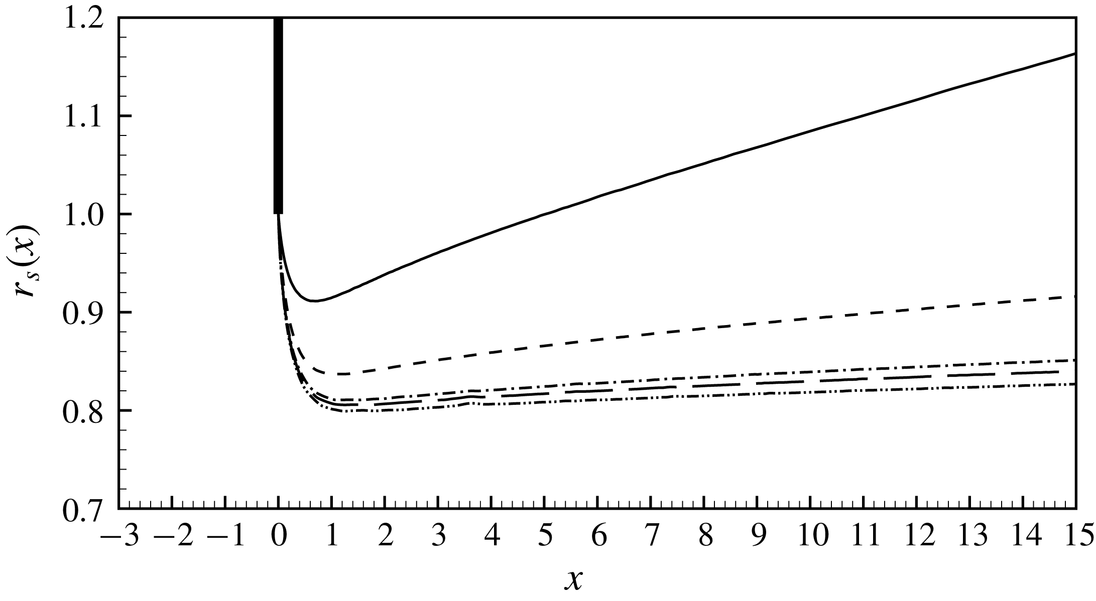
The radius of the shear layer
 $r_{s}(x)$
can be extracted from the base-flow fields by localizing the streamline growing up from the edge of the hole. The actual shape of the jet has a great influence on the calculation of the impedance and many analytical models are based on its reconstruction from experimental or numerical data (Jing & Sun Reference Jing and Sun2000; Mendez & Eldredge Reference Mendez and Eldredge2009; Yang & Morgans Reference Yang and Morgans2016). We reported our results in figure 5 for various Reynolds numbers. For
 $Re=100$
the jet is not parallel: the inertia of the flow is low and the jet is accelerated only for a short distance; then, the effect of viscosity leads to a diffusion of the jet. For higher Reynolds numbers, instead, the inertial effects dominate the system: the fluid is accelerated for a long distance and the radius of the jet diverges very far (not reported here). Moreover, it is very clear that the jet is almost parallel and for high Reynolds numbers the radius of the jet is approximately
 $R_{J}\approx 0.8$
.
Vena contracta coefficient as a function of
 $Re$
. The circles (○) indicate the values of the vena contracta coefficient corresponing to the Reynolds number reported in figure 5.
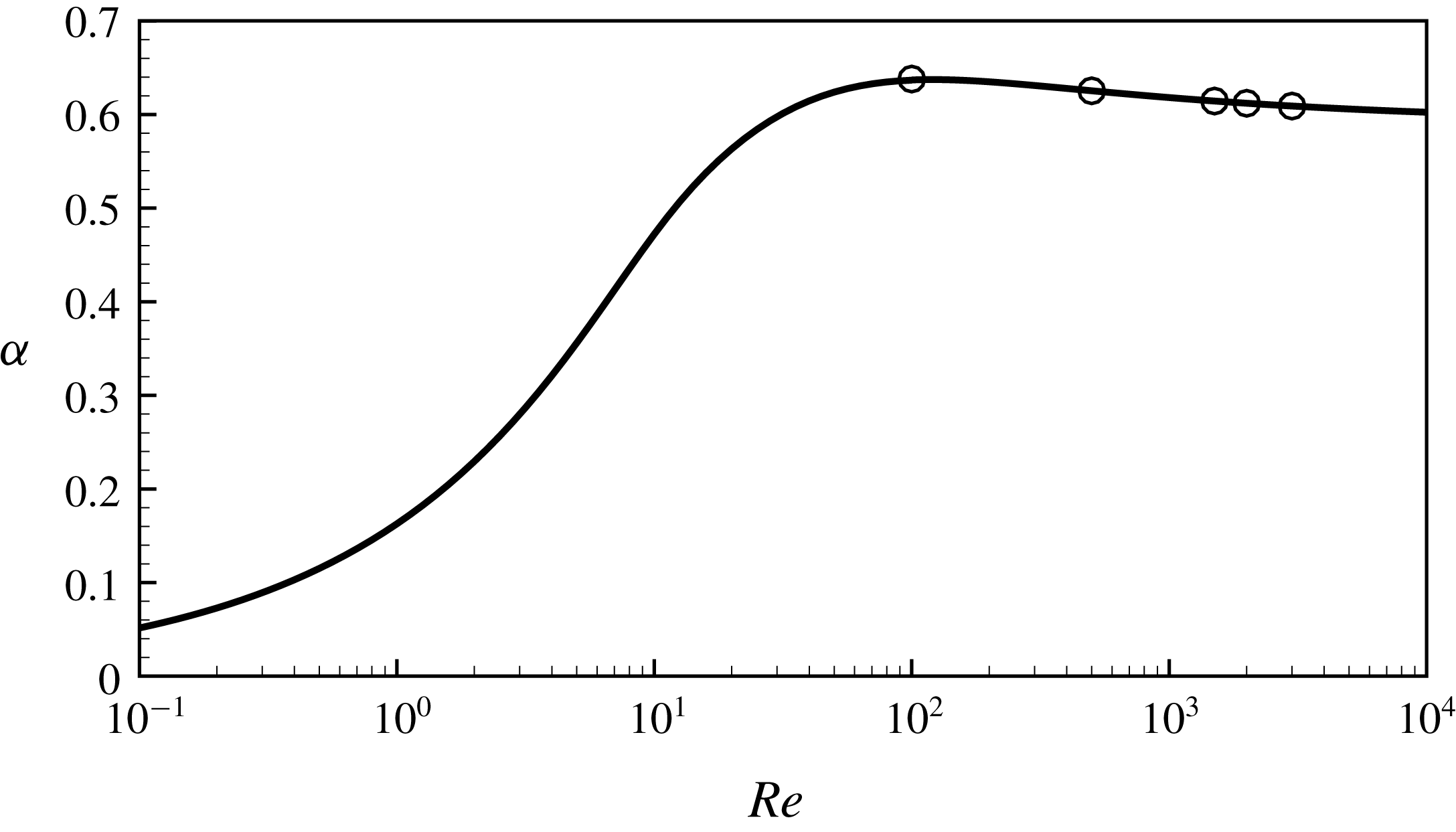
As recalled in § 2.2, this effect is classically measured through the introduction of the vena contracta coefficient
 $\unicode[STIX]{x1D6FC}$
which is directly related to the pressure drop
 $[P_{in}-P_{out}]$
. We calculated the vena contracta coefficient by inverting the equation (2.4) as a function of the Reynolds number. The results are shown in figure 6: we note that the curve grows with the Reynolds number, then it reach a maximum at
 $Re\approx 120$
and then it assumes an asymptotic behaviour as
 $Re\rightarrow \infty$
, leading to
 $\unicode[STIX]{x1D6FC}\approx 0.61$
, which is in agreement with classical results (Smith & Walker Reference Smith and Walker1923). Finally, we estimated the radius of the ideal jet at large Reynolds number using the relation
 $R_{J}\approx R_{h}\sqrt{\unicode[STIX]{x1D6FC}}\approx 0.78$
, where
 $\unicode[STIX]{x1D6FC}$
is the classically assumed
 $0.61$
: this value is in very good agreement with the value
 $R_{J}\approx 0.8$
extracted from the figure 5.
5 Results for the unsteady flow
5.1 Structure of the unsteady flow for
$Re=500$

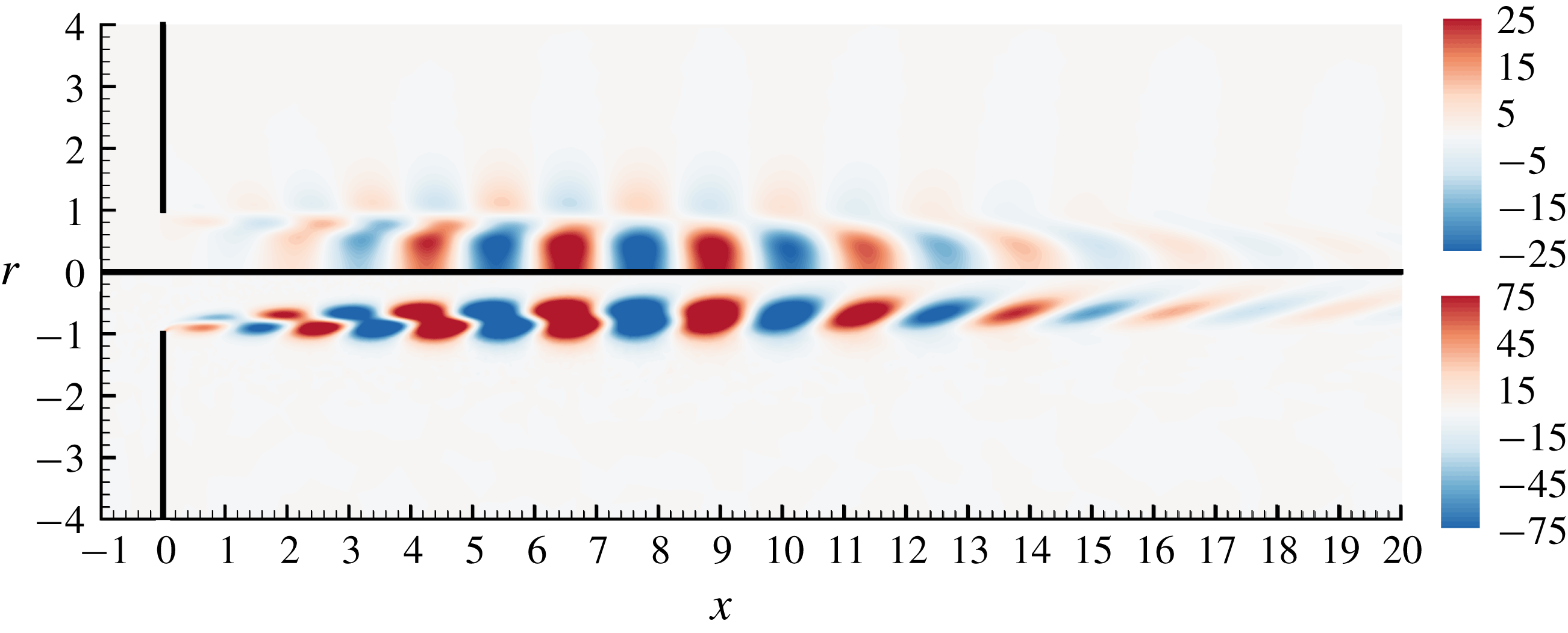
Let us now investigate the structure of the flow perturbation due to harmonic forcing. Figure 7 displays this structure for a moderate value of the Reynolds number, namely
 $Re=500$
, and for
 $\unicode[STIX]{x1D6FA}=3$
, computed in physical coordinates without mapping (mesh
 $\mathbb{M}_{0}$
). As can be observed, the effect of a periodic forcing is to generate vortical structures in the jet which are amplified and convected in the downstream direction. In the case plotted, the maximum level is reached at approximately
 $x\approx 8$
. Progressing further downstream, the perturbations are no longer amplified but begin to slowly decrease, until they vanish for
 $x\gtrsim 20$
. This is consistent with the fact that for
 $x\gtrsim 8$
the shear layer bounding the jet has diffused (as documented in figure 3
b) and is not steep enough to sustain a spatial instability.
Harmonic perturbation for
 $\text{Re}=500,\unicode[STIX]{x1D6FA}=3$
computed in physical coordinates
 $(x,r)$
(mesh
 $\mathbb{M}_{0}$
). Real part of the axial velocity component
 $u_{x}^{\prime }$
(upper) and vorticity
 $\unicode[STIX]{x1D709}^{\prime }$
(lower).
Harmonic perturbation for
 $\text{Re}=500,\unicode[STIX]{x1D6FA}=3$
(in physical coordinates
 $(x,r)$
; mesh
 $\mathbb{M}_{0}$
) on the axis of symmetry. Real (——) and imaginary (– –) part of the axial velocity component
 $u_{x}^{\prime }$
(thin lines) and pressure
 $p^{\prime }$
(thick lines).
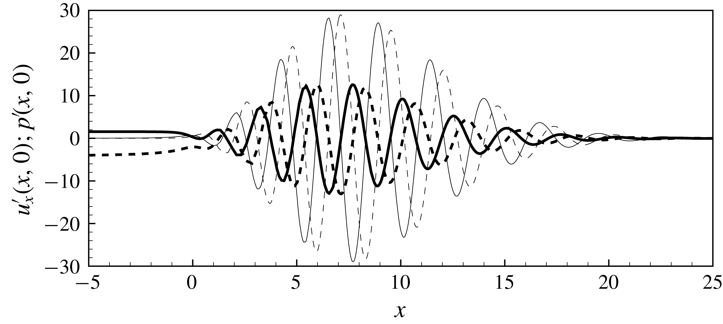
In figure 8 we display the values taken along the axis of the jet of the axial velocity
 $u_{x}^{\prime }(x,0)$
and the pressure
 $p^{\prime }(x,0)$
associated with the harmonic perturbation previously described. One can clearly observe that the pressure perturbation asymptotes to different limit values in the upstream and downstream domains, allowing us to deduce the pressure jump
 $[p_{in}^{\prime }-p_{out}^{\prime }]$
which is the key parameter allowing us to define the impedance and/or the conductivity. In the upstream region the asymptote is reached rapidly and the pressure is almost constant with
 $p^{\prime }(x,0)\approx p_{in}^{\prime }=1.8-3i$
for
 $x\lesssim -3$
. On the other hand, in the downstream region, the asymptotic limit (which amounts to
 $p_{out}^{\prime }=0$
owing to the way the boundary conditions are introduced in the problem, see § 3) is only reached for
 $x\gtrsim 25$
, after the spatial growth and subsequent decay.
Harmonic perturbation for
 $\text{Re}=500,\unicode[STIX]{x1D6FA}=3$
(in numerical coordinates
 $(X,R)$
with complex mapping; mesh
 $\mathbb{M}_{1}$
). Real part of the axial velocity component
 $u_{x}^{\prime }$
(upper) and vorticity (lower).
5.2 Efficiency of the complex mapping technique
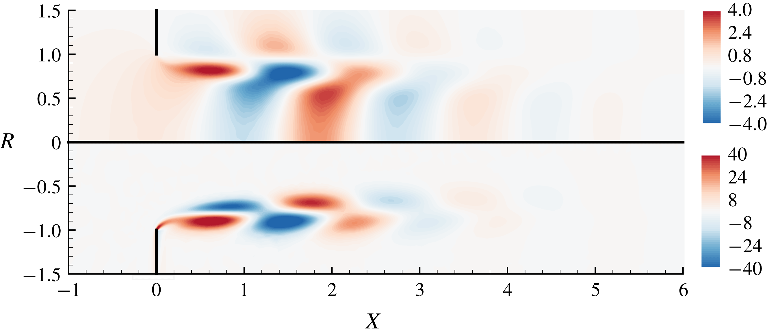
Figure 9 displays the structure of the perturbation for the same parameters as in figure 7, but using the complex mapping technique (with mesh
 $\mathbb{M}_{1}$
). Accordingly, the structure is plotted as function of the (real) numerical coordinates
 $[X,R]$
. As one can observe, the complex mapping technique completely fulfils the goal of getting rid of the strong spatial amplification in the downstream direction.
Of course, the spatial structure displayed in figure 9 has no physical meaning as soon as
 $X>0$
, because a point
 $(X,R)$
in the numerical domain corresponds to a point
 $(x,r)$
in the physical domain for some complex
 $x$
defined by
 $x=G(X)$
, and there is no easy way to access the structure of the perturbation for some real
 $x$
. However, since our focus is on the impedance of the jets, we are not interested in a full characterization of the perturbation field but only by a determination of the associated pressure jump.
(a) Pressure contours of the perturbation
 $p^{\prime }$
computed in physical coordinates (mesh
 $\mathbb{M}_{0}$
; upper part) and with the complex mapping (mesh
 $\mathbb{M}_{1}$
; lower part). (b) Pressure of the perturbation on the symmetry axis
 $p^{\prime }(X,0)$
with (——) and without (– –) the complex mapping (
 $Re=500$
;
 $\unicode[STIX]{x1D6FA}=3$
).
Same as figure 10(a,b) but for
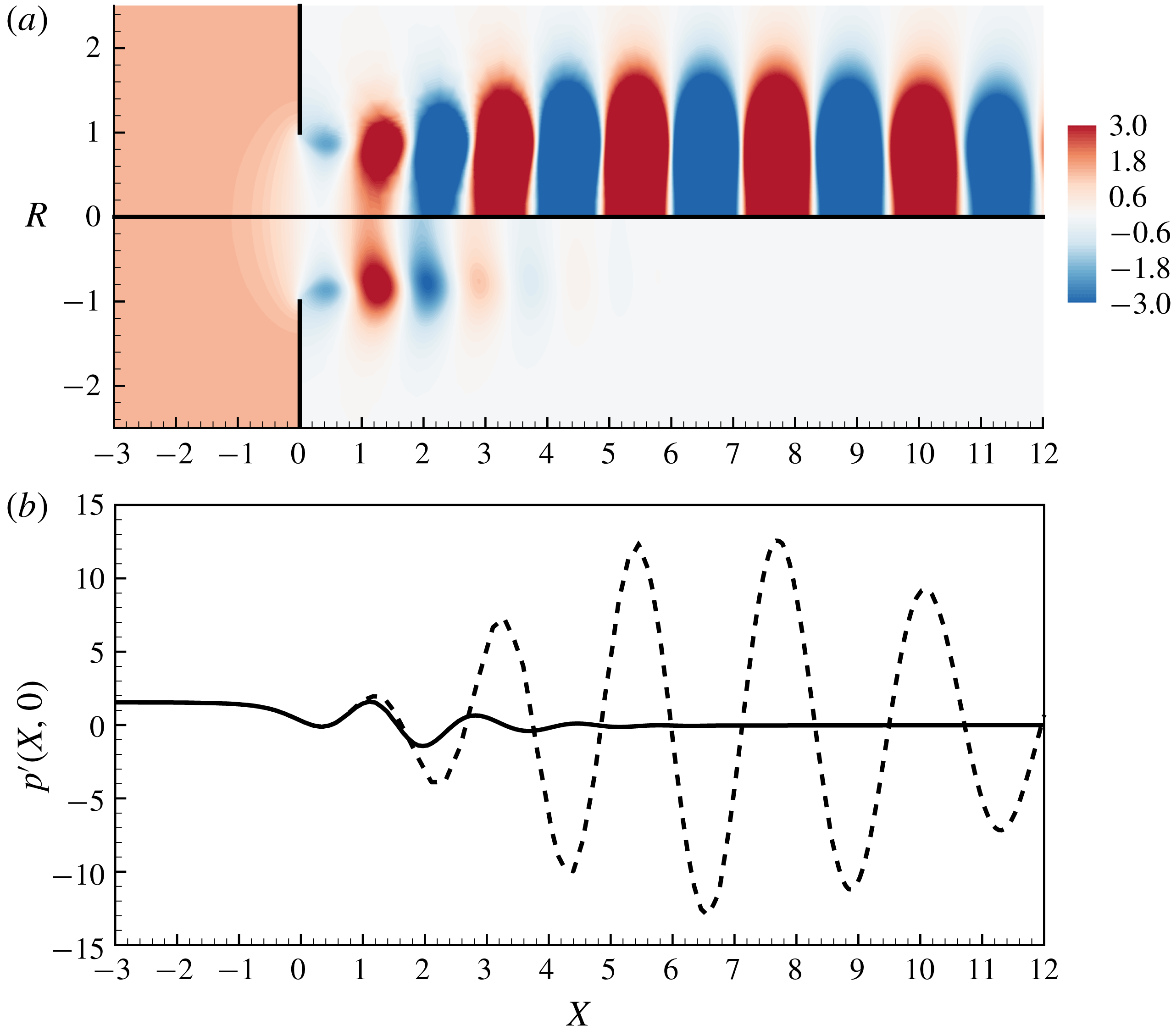
 $Re=1000$
. The inset (c) displays a zoom in the near hole region in order to catch the pressure jump across the hole.
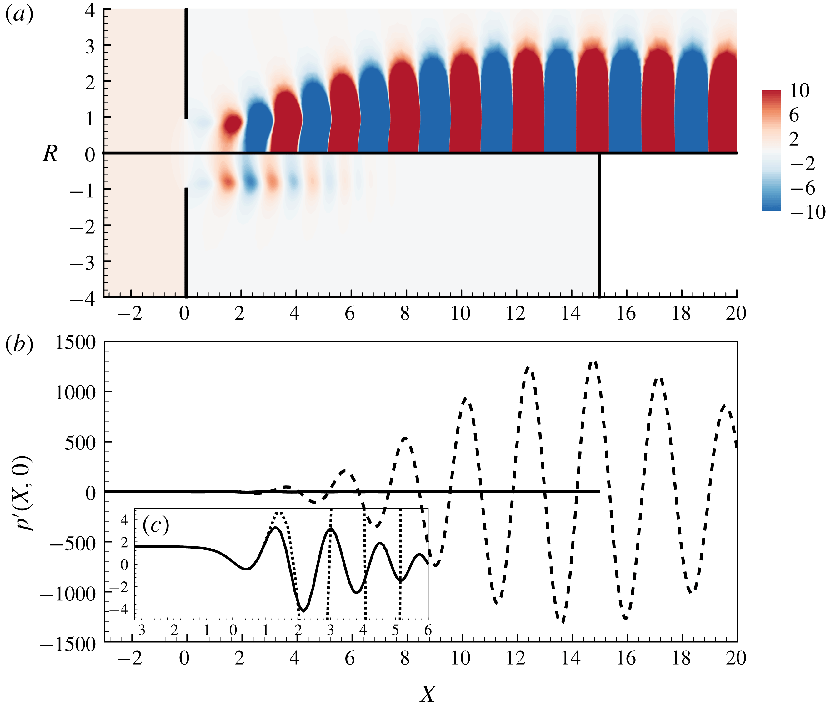
Figure 10 compares the results obtained with and without complex mapping (again for
 $\text{Re}=500$
and
 $\unicode[STIX]{x1D6FA}=3$
), focussing on the pressure component
 $p^{\prime }$
(real part) of the harmonic disturbance. In figure 10(a) the same iso-levels are used for both results without complex mapping (upper half) and with complex mapping (lower half). The comparison shows again that the structure computed without complex mapping quickly grows to reach large values, saturating the iso-levels, while the structure computed with complex mapping nicely decays to rapidly reach zero. Figure 10(b) complements the comparison with plots of the pressure field along the axis. The comparison confirms that in the inlet region (
 $X<0$
) the results exactly coincide. For
 $0<X\lesssim 1.25$
the results with complex mapping remain qualitatively similar to the ones without mapping while for
 $X\gtrsim 1.25$
they become completely different and rapidly decay to zero. This not surprising, as our definition the mapping function defining our mesh contains a parameter
 $L_{C}=1.25$
such that for
 $X<L_{C}$
the corresponding physical variable
 $x=G_{x}(X)$
is almost real while for
 $X>L_{C}$
it is fully complex.
Let us now consider the case
 $\text{Re}=1000$
,
 $\unicode[STIX]{x1D6FA}=3$
. The pressure
 $p^{\prime }$
of the harmonic disturbance is plotted in figure 11(a,b), with the same conventions as in figure 10. Inspection shows that the results without complex mapping lead to the same difficulties as for
 $Re=500$
but the spatial growth is much more pronounced. In this case, the pressure levels reach an amplitude of order
 $10^{3}$
for
 $x\approx 15$
and the asymptotic value
 $p_{out}^{\prime }=0$
is only reached for
 $x\gtrsim 70$
. This justifies that fact that, to correctly resolve this mode, we had to design the dimension of the mesh
 $\mathbb{M}_{0}$
to be as large as
 $L_{out}=80$
. On the other hand, results obtained with complex mapping behave very similarly as for
 $Re=500$
, and the asymptotic limit
 $p_{out}^{\prime }=0$
is reached quite rapidly, for
 $X\gtrsim 8$
.
In figure 11(b), the pressure levels of the results with and without complex mapping are so different that it is impossible to check that the pressure
 $p^{\prime }$
effectively asymptotes to the same limits
 $p_{in}^{\prime }$
and
 $p_{out}^{\prime }$
in both cases. To remedy this, figure 11(c) shows a zoom of the results in figure 11(b), in the region close to the hole. This representation confirms that the two computations lead to identical results in the upstream region where no mapping is used (and in particular that the upstream limit
 $p_{in}^{\prime }$
is the same), and that for the case using complex mapping the downstream limit is reached after only a few oscillations with amplitudes of order one.
Figures 10 and 11 thus confirm that the use of complex mapping is a convenient and efficient way to access to the pressure jump
 $p_{in}^{\prime }-p_{out}^{\prime }$
associated with the harmonic perturbation without having to deal with the strong spatial amplifications. It is worth pointing out that in this method is also computationally economical, as the number of point in mesh
 $\mathbb{M}_{1}$
is approximately half that of the unmapped case
 $\mathbb{M}_{0}$
. The figures also indicate that the difficulties encountered when solving the problem in physical coordinates without mapping become worse as the Reynolds number becomes large. In practice, as soon as
 $Re\gtrsim 1500$
, the huge levels reached by the perturbations in the far-field region lead to round-off errors and it becomes impossible to accurately resolve the near-field region. We verified that enlarging the domain of dimension
 $L_{out}$
to even larger than 80 does not improve the results. Using ‘sponge’ regions with artificially large viscosity was also tried as an alternative idea to get rid of the problems associated with huge spatial amplifications, but this idea proved to be unsuccessful. In the end the only efficient way we found to obtain reliable results for
 $Re\gtrsim 1500$
was to use the complex mapping technique. An illustration of the failure of the resolution in physical variables for large Reynolds is given in § B.1 (figures 20 and 21).
Note that in order to be consistent, the base flow also needs to be computed with the same numerical coordinates. The structure of the base flow in mapped coordinates has no physical meaning for the same reasons as the harmonic perturbation, but we verified that the pressure jump and the associated vena contracta coefficient are identical to the results in physical coordinates. We detail this in appendix C, and display an example of base flow obtained in such a way in figure 25.
5.3 Impedance and conductivity
Having illustrated the structure of the perturbation due to a harmonic forcing and justified the validity of the numerical method, we now come to the most important result of this work, namely prediction of the impedance as function of
 $Re$
and
 $\unicode[STIX]{x1D6FA}$
.
(a) Resistance
 $Z_{R}$
and (b) reactance
 $-Z_{I}/\unicode[STIX]{x1D6FA}$
for
 $Re=100$
(——),
 $Re=500$
(– –),
 $Re=1500$
(— ⋅ —),
 $Re=2000$
(— —) and
 $Re=3000$
(— ⋅ ⋅ —).
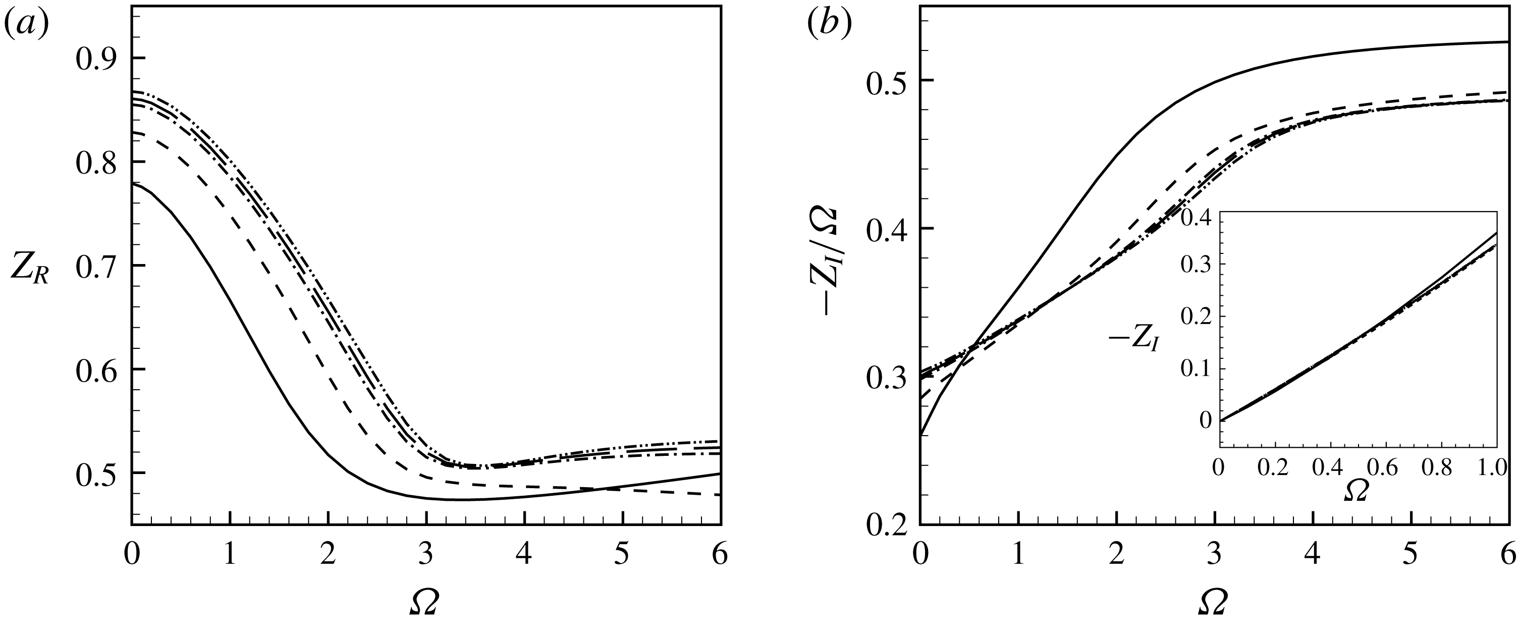
Figure 12 displays the real and imaginary parts of the impedance, calculated according to equation (2.8), as a function of the forcing frequency
 $\unicode[STIX]{x1D6FA}$
at various Reynolds numbers.
As for the resistance (panel
 $a$
), only the case
 $Re=100$
is notably different from the other ones. On the other hand, the results obtained for
 $Re>1500$
seem to collapse in a unique curve, indicating that a large Reynolds number asymptotic regime is attained after this value. The resistance is maximum in the low-frequency limit
 $\unicode[STIX]{x1D6FA}\approx 0$
, with a value
 $Z_{R}\approx 0.85$
which will be explained in the next section. As
 $\unicode[STIX]{x1D6FA}$
is increased,
 $Z_{R}$
first decreases to reach a minimum for
 $\unicode[STIX]{x1D6FA}\approx 3.5$
and then it reaches a quasi-constant value equal to
 $0.53$
. Moreover, one can observe that the resistance increases with the Reynolds number for all values of the frequency
 $\unicode[STIX]{x1D6FA}$
. One can note that the resistance is always positive, meaning that, according to equation (2.10), the jet is an energy sink and so, in order to excite the jet at a given frequency, we need to provide energy from an outer system, as recently observed by Howe (Reference Howe1979) for an inviscid flow.
The reactance
 $Z_{I}$
is documented in panel (
 $b$
). As this quantity turns out to be a negative and approximately linear function of
 $\unicode[STIX]{x1D6FA}$
, it is more practical to plot
 $-Z_{I}/\unicode[STIX]{x1D6FA}$
as a function of
 $\unicode[STIX]{x1D6FA}$
. Under this representation, we can make the same observation as for the resistance, regarding the existence of a high Reynolds number asymptotic regime for
 $Re\gtrsim 1500$
, and the notable difference of the case
 $Re=100$
. Note that in the high-frequency range, the curves indicate an asymptotic trend given by
 $Z_{I}/\unicode[STIX]{x1D6FA}\approx 0.5$
. This value matches with that predicted by the simple Rayleigh model (§ 2.3), indicating that, for large frequencies, the impedance of the hole is at leading order the same as in the absence of a mean flow.
We now document the results using the equivalent concept of conductivity (see § 2.2), and compare these with the predictions of Howe’s model. Just as for the impedance, the results for
 $Re\gtrsim 1500$
collapse onto a single curve characterizing a high Reynolds number asymptotic regime. In figure 13 we plot with a thick line the results obtained for
 $Re=3000$
which are representative of this regime.
(a) Real part
 $\unicode[STIX]{x1D6FE}$
and (b) imaginary part
 $\unicode[STIX]{x1D6FF}$
of the Rayleigh conductivity. Plain lines: LNSE results for
 $\text{Re}=3000$
. Dash-dotted lines: Howe’s original model. Dotted lines: Howe’s modified model.
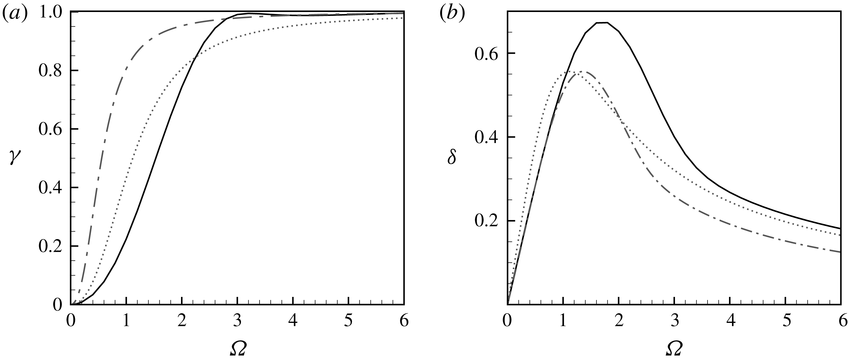
As explained in § 2.5, Howe’s expression for the conductivity (2.13) is expressed in terms of
 $\unicode[STIX]{x1D6FA}^{H}=\unicode[STIX]{x1D714}R_{h}/U_{c}$
where
 $U_{c}$
is the convection velocity of the structures along the vortex sheet, which choice is one of the most questionable points of the analysis. In the initial model, Howe disregarded the vena contracta phenomenon and assumed a jet with radius
 $R_{h}$
and velocity
 $U_{J}=U_{M}$
. Then, assuming
 $U_{c}=U_{M}/2$
leads to
 $\unicode[STIX]{x1D6FA}^{H}=2\unicode[STIX]{x1D6FA}$
. The values for
 $\unicode[STIX]{x1D6FE}$
and
 $\unicode[STIX]{x1D6FF}$
obtained with this choice are plotted in the figure with dash-dotted lines. As can be seen, in this initial version, Howe’s model rather badly agrees with our LNSE results. In a subsequent step of his analysis, Howe argued that the effect of the vena contracta can be partly accounted for by using the more appropriate choice
 $U_{J}=2U_{M}$
. This choice leads to
 $U_{c}=U_{M}$
and hence
 $\unicode[STIX]{x1D6FA}^{H}=\unicode[STIX]{x1D6FA}$
. The predictions of this modified model are plotted by the dashed lines in the figure. As can be seen, the agreement with LNSE results is improved but the curves still differ notably, especially as for the imaginary part
 $\unicode[STIX]{x1D6FF}$
(panel
 $b$
) in the range
 $\unicode[STIX]{x1D6FA}\approx 2$
where Howe’s modified model underestimates the numerically computed one by approximately
 $30\,\%$
. On the other hand, the model overestimates the real part
 $\unicode[STIX]{x1D6FE}$
for
 $\unicode[STIX]{x1D6FA}\lesssim 2$
by approximately
 $10\,\%$
and underestimates it for
 $\unicode[STIX]{x1D6FA}\gtrsim 2$
by the same amount.
As discussed in § 2.5, the result of Howe is expressed in terms of a non-dimensional frequency
 $\unicode[STIX]{x1D6FA}^{H}=\unicode[STIX]{x1D6FA}R_{h}/U_{c}$
based on the convection velocity of vorticity structures along the vortex sheet
 $U_{c}$
, whose precise value is questionable. In figure 13 we followed the original choice of Howe
 $U_{c}=U_{M}$
which leads to
 $\unicode[STIX]{x1D6FA}^{H}=\unicode[STIX]{x1D6FA}$
. We also tried to compare the results using improved modellings of
 $U_{c}$
, leading only to mild ameliorations of the agreement.
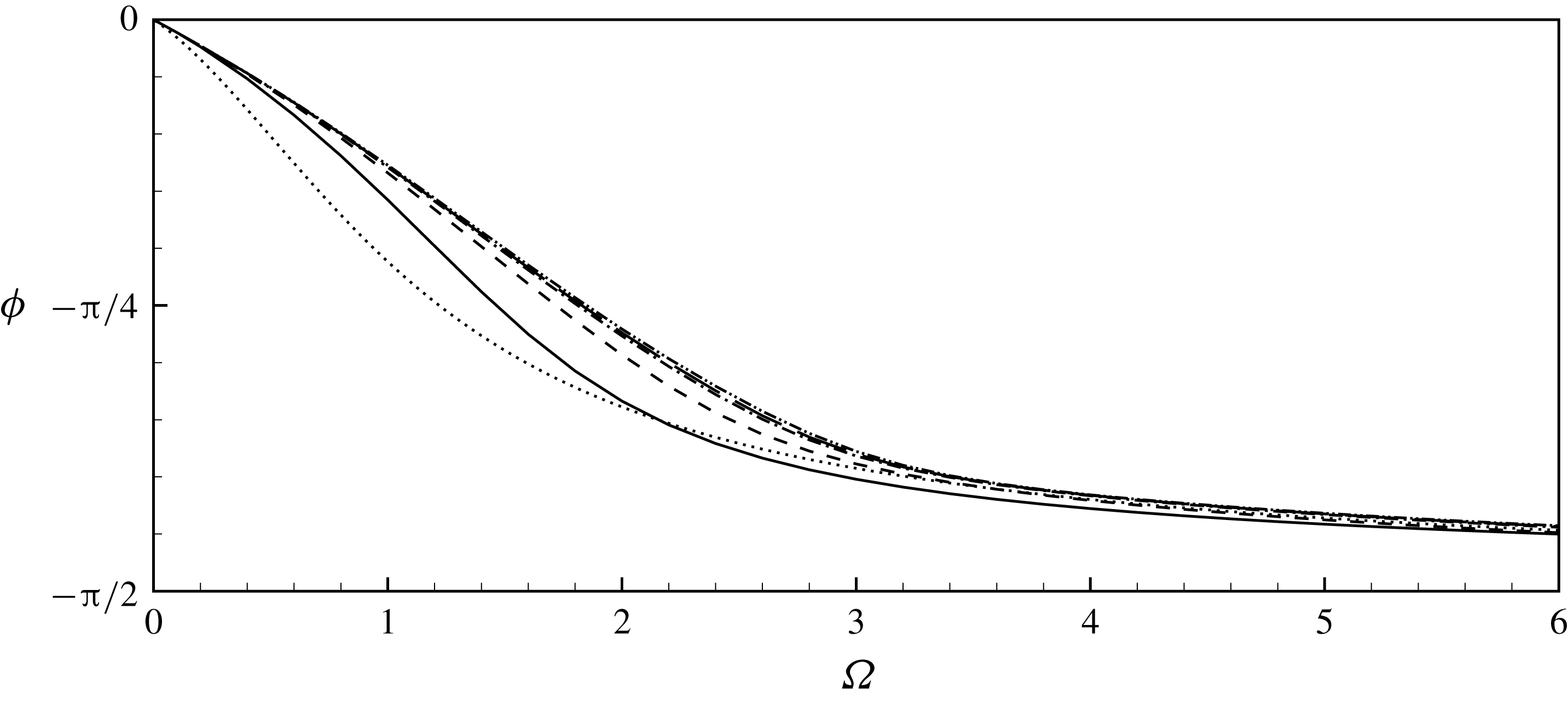
Argument
 $\unicode[STIX]{x1D719}$
of the impedance, for
 $Re=100$
(——),
 $Re=500$
(– –),
 $Re=1500$
(— ⋅ —),
 $Re=2000$
(— —) and
 $Re=3000$
(— ⋅ ⋅ —), and from Howe’s modified model
 $(\cdots )$
.
Finally, a useful quantity which can be extracted from the impedance is the delay angle of the pressure with respect to the velocity:
 $$\begin{eqnarray}\unicode[STIX]{x1D719}=\text{arg}(Z_{h})=\tan ^{-1}\left(\frac{Z_{I}}{Z_{R}}\right)\!.\end{eqnarray}$$
This quantity has been used in a number of experiments, as it allows us to discriminate the cases where the impedance is mainly resistive (
 $\unicode[STIX]{x1D719}\approx 0$
) from the ones where it is mainly reactive (
 $\unicode[STIX]{x1D719}\approx -\unicode[STIX]{x03C0}/2$
). This quantity is plotted in figure 14, confirming that the behaviour switches from purely resistive to purely reactive as the frequency is increased. We also observe in this plot a collapse of the curves obtained in the high Reynolds number asymptotic regime
 $Re\gtrsim 1500$
. The angle
 $\unicode[STIX]{x1D719}$
extracted from Howe’s modified model is also plotted in the figure (note that in terms of conductivity, the definition of
 $\unicode[STIX]{x1D719}$
translates into
 $\unicode[STIX]{x1D719}=\unicode[STIX]{x03C0}/2-\text{arg}(K_{R})=-\text{tan}^{-1}(\unicode[STIX]{x1D6FE}/\unicode[STIX]{x1D6FF})$
). Again, a substantial deviation is observed, especially in the range of intermediate frequencies
 $\unicode[STIX]{x1D6FA}\approx 2$
where the deviation can be as large as
 $\unicode[STIX]{x03C0}/12\equiv 15^{\circ }$
. Oddly, the inviscid Howe model turns out to give better predictions for the case
 $Re=100$
than for the high Reynolds number regime.
5.4 The quasi-static limit for
$\unicode[STIX]{x1D6FA}\rightarrow 0$

We have observed that in the limit of small frequencies (
 $\unicode[STIX]{x1D6FA}\rightarrow 0$
), the impedance becomes purely real and tends to a constant value. This limit value can be predicted using a quasi-static approximation, and this property will be used to verify the consistency of our impedance calculations. As explained in § 2.3 for a steady flow, the pressure jump and the mean velocity across the hole are related through the Bernoulli equation which can be written in the form (2.4)
 $$\begin{eqnarray}\unicode[STIX]{x0394}p=\frac{\unicode[STIX]{x1D70C}u_{M}^{2}}{2\unicode[STIX]{x1D6FC}^{2}(Re_{M})}.\end{eqnarray}$$
Assuming
 $\unicode[STIX]{x0394}p=\unicode[STIX]{x0394}P+\unicode[STIX]{x0394}p^{\prime }$
and
 $u_{M}=U_{M}+u_{M}^{\prime }$
, inserting into (5.2) with
 $Re_{M}=(U_{M}+u_{M}^{\prime })R_{h}/\unicode[STIX]{x1D708}=Re(1+u_{M}^{\prime }/U_{M})$
and linearizing leads to
 $$\begin{eqnarray}\unicode[STIX]{x0394}P+\unicode[STIX]{x0394}p^{\prime }\approx \frac{\unicode[STIX]{x1D70C}U_{M}^{2}}{2\unicode[STIX]{x1D6FC}^{2}}+\frac{\unicode[STIX]{x1D70C}u_{M}^{\prime }U_{M}}{\unicode[STIX]{x1D6FC}^{2}}\left(1-\frac{1}{\unicode[STIX]{x1D6FC}}\frac{\unicode[STIX]{x2202}\unicode[STIX]{x1D6FC}}{\unicode[STIX]{x2202}Re}\right)\!.\end{eqnarray}$$
Remembering now that
 $\unicode[STIX]{x0394}P=(\unicode[STIX]{x1D70C}U_{M}^{2})/(2\unicode[STIX]{x1D6FC}^{2})$
, this equation allows us to obtain a prediction for the impedance which is assumed to be valid in the quasi-static limit (
 $\unicode[STIX]{x1D6FA}\rightarrow 0$
):
 $$\begin{eqnarray}Z_{QS}=\frac{\unicode[STIX]{x0394}p^{\prime }}{\unicode[STIX]{x03C0}R_{h}^{2}u_{M}^{\prime }}=\frac{\unicode[STIX]{x1D70C}U_{M}}{\unicode[STIX]{x1D6FC}^{2}\unicode[STIX]{x03C0}R_{h}^{2}}\left(1-\frac{1}{\unicode[STIX]{x1D6FC}}\frac{\unicode[STIX]{x2202}\unicode[STIX]{x1D6FC}}{\unicode[STIX]{x2202}Re}Re\right)\!.\end{eqnarray}$$
Table 1 compares the impedance computed using the method of the previous section for a small value of the frequency, namely
 $\unicode[STIX]{x1D6FA}=10^{-6}$
, to the quasi-static prediction (5.4) obtained using the base-flow characteristics computed in § 4. One can note that the results agree with a less than
 $1\,\%$
error. Finally, we can note that the term
 $(1/\unicode[STIX]{x1D6FC})(\unicode[STIX]{x2202}\unicode[STIX]{x1D6FC}/\unicode[STIX]{x2202}Re)Re$
in (5.4) is small because
 $\unicode[STIX]{x1D6FC}$
is a slowly varying function of
 $Re$
. The fourth column of table 1 gives the prediction of the quasi-static impedance obtained when neglecting this term. The comparison shows that this simplified prediction is still an excellent approximation, and slightly overestimates the actual value, except for the case
 $Re=100$
, where it underestimates it. This is consistent with the fact that the
 $\unicode[STIX]{x1D6FC}-Re$
curve reaches a maximum for
 $Re\approx 120$
(see figure 6).
The low-frequency limit was also addressed by Howe in the framework of his model. A Taylor series of expression (2.13) leads to
 $\unicode[STIX]{x1D6FF}\approx \unicode[STIX]{x03C0}\unicode[STIX]{x1D6FA}^{H}/4$
(equation 3.15(b) of Howe’s paper), which, when expressed in terms of impedance, translates into
 $Z_{R}\approx (2/\unicode[STIX]{x03C0})(U_{c}/U_{M})\approx 0.637(U_{c}/U_{M})$
. Thus, the choice
 $U_{c}/U_{M}=1$
made by Howe actually yields a prediction for
 $Z_{R}$
which underestimates the high Reynolds number value by approximatively
 $37\,\%$
. Note that this mismatch can also be observed in figure 13(b) regarding the initial slope of the curve
 $\unicode[STIX]{x1D6FF}(\unicode[STIX]{x1D6FA})$
. This error in the quasi-static limit may be cancelled using an ad hoc choice of
 $U_{c}/U_{M}$
, but as previously explained, such a modification does not improve substantially the agreement in other ranges of
 $\unicode[STIX]{x1D6FA}$
.
Values of the impedance in the low-frequency range. Comparison of values obtained numerically with a very small
 $\unicode[STIX]{x1D6FA}$
, quasi-static approximation (5.4) and simplified approximation obtained assuming
 $\unicode[STIX]{x2202}\unicode[STIX]{x1D6FC}/\unicode[STIX]{x2202}Re=0$
.
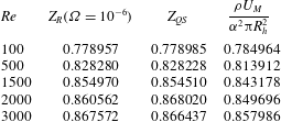
6 Direct numerical simulations of a harmonically forced jet
In order both to validate the linearized approach for small amplitudes and to investigate the influence of nonlinearities for larger amplitudes, we performed direct numerical simulations by integrating in time the Navier–Stokes equations (3.1) for a harmonically forced jet. The DNS are performed using FreeFem++ on the same mesh
 $\mathbb{M}_{0}$
as used in the previous section for resolution in physical coordinates (note that the complex mapping technique is fitted to the resolution of the linearized problem but is not relevant for nonlinear simulations). The numerical code used for time integration is very similar to the one used in Marquet et al. (Reference Marquet, Sipp, Chomaz and Jacquin2008). The equations are advanced in time using a partly implicit second-order accurate scheme. The time derivatives are approximated using a three-step backward finite difference scheme. The pressure, the Laplacian term and the continuity equation are implicit while the convective terms are explicit and treated using a characteristics method (Boukir et al.
Reference Boukir, Maday, Métivet and Razafindrakoto1997).
As initial conditions, we used the steady solution of the Navier–Stokes equations
 $[\boldsymbol{U};P]$
obtained as described in § 3.4. We used the same boundary conditions as for the LNSE, namely no stress on
 $\unicode[STIX]{x1D6E4}_{w}$
, symmetry on
 $\unicode[STIX]{x1D6E4}_{axis}$
, stress-free conditions on
 $\unicode[STIX]{x1D6E4}_{lat}$
and traction free on
 $\unicode[STIX]{x1D6E4}_{out}$
. At the inflow, we forced the problem on the axial velocity component as follows:
 $$\begin{eqnarray}\left.\begin{array}{@{}c@{}}\displaystyle u_{x}(t)=U_{in}[1+\unicode[STIX]{x1D700}\sin (\unicode[STIX]{x1D714}t)]\\ \displaystyle u_{r}=0\end{array}\right\}\quad \text{on }\unicode[STIX]{x1D6E4}_{in},\end{eqnarray}$$
where
 $U_{in}=Q/S_{in}$
and
 $Q$
has been selected as just discussed in § 3.2. The pressure drop
 $\unicode[STIX]{x0394}p(t)$
necessary to define the impedance is then extracted using
 $$\begin{eqnarray}\unicode[STIX]{x0394}p(t)=p_{in}(t)-p_{out}(t)=2\unicode[STIX]{x03C0}/S_{in}\int _{0}^{R_{in}}p(r,t)r\,\text{d}r-2\unicode[STIX]{x03C0}/S_{out}\int _{0}^{R_{out}}p(r,t)r\,\text{d}r.\end{eqnarray}$$
For the simulations, we fixed the Reynolds number to
 $Re=1000$
and investigated the effect of both the frequency in the range
 $\unicode[STIX]{x1D6FA}\in [0.5-4]$
and the amplitude in the range
 $\unicode[STIX]{x1D700}\in [10^{-4},10^{-1}]$
.
Vorticity snapshot at (a)
 $\unicode[STIX]{x1D6FA}=0.5$
, (b)
 $\unicode[STIX]{x1D6FA}=2$
, (c)
 $\unicode[STIX]{x1D6FA}=4$
for
 $\unicode[STIX]{x1D700}=10^{-2}$
,
 $Re=1000$
and
 $t=25$
. The line with arrows is the edge of the jet, i.e. the streamline originating from the edge of the hole.
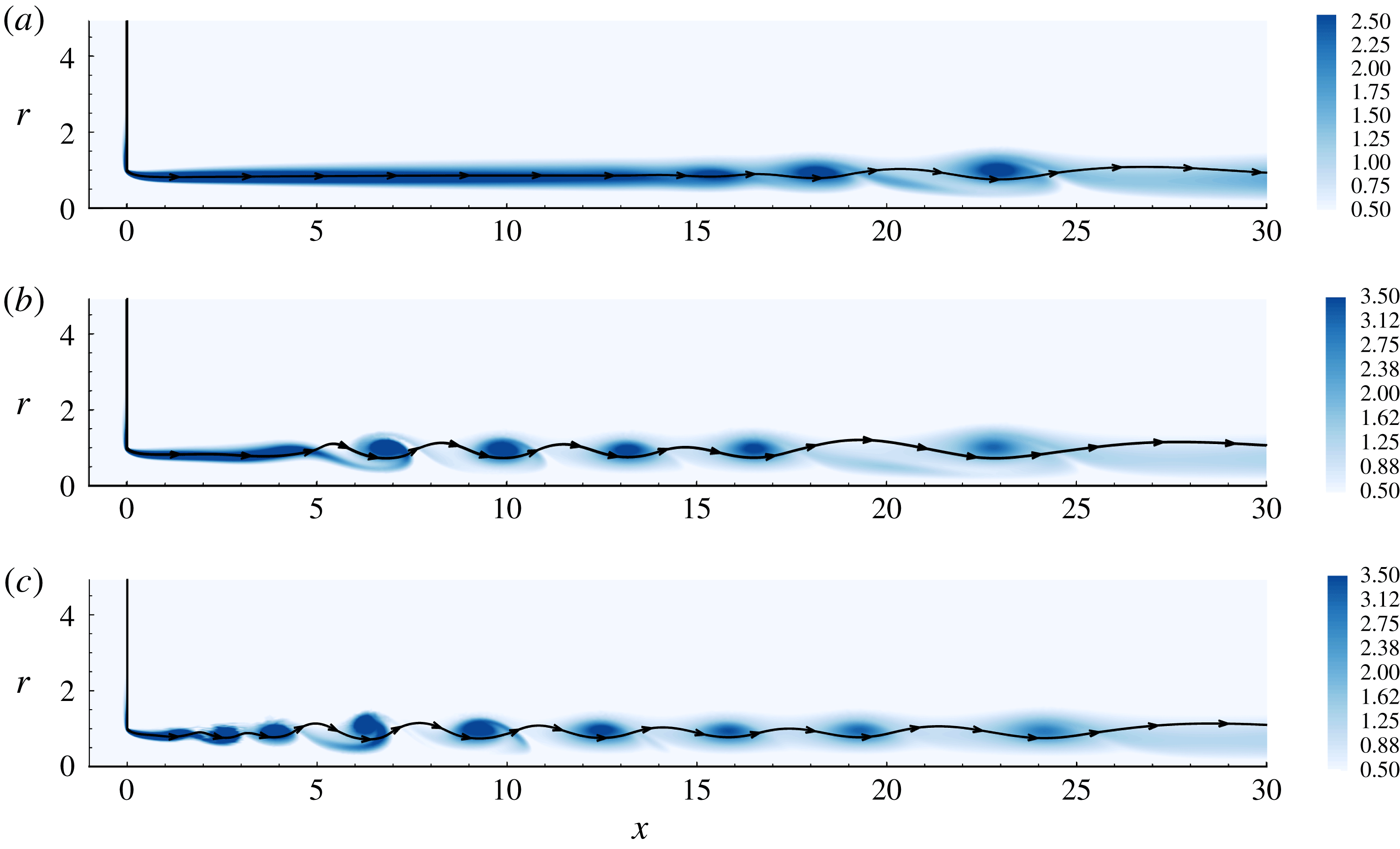
Figure 15 displays a snapshot of the vorticity for
 $\unicode[STIX]{x1D700}=10^{-2}$
and
 $\unicode[STIX]{x1D6FA}=0.5$
,
 $2$
and
 $4$
. We also display the streamline originating from the edge of the hole, which can be identified with the surface of the jet
 $\unicode[STIX]{x1D702}(x,t)$
of figure 1. We can observe that, under the effect of forcing, the shear layer bounding the jet reorganises into an array of vortices which are convected downstream. Note that the distance at which the vortex array appears is much larger in the lower-frequency case, because the spatial instability of the jet is less active at low frequencies. The overall structure of the vorticity is consistent with studies which have used DNS of a harmonically forced to characterize the spatial amplification process (Kiya, Ido & Akiyama Reference Kiya, Ido and Akiyama1996; Shaabani-Ardali, Sipp & Lesshafft Reference Shaabani-Ardali, Sipp and Lesshafft2017).
Time series of the pressure drop
 $\unicode[STIX]{x0394}p(t)$
and the velocity at
 $(x,r)=(10,0.5)$
for
 $\unicode[STIX]{x1D6FA}=0.5$
(a,b) and
 $\unicode[STIX]{x1D6FA}=2$
(c,d). Full line is for
 $\unicode[STIX]{x1D700}=0.1$
and dashed line is for
 $\unicode[STIX]{x1D700}=0.05$
.
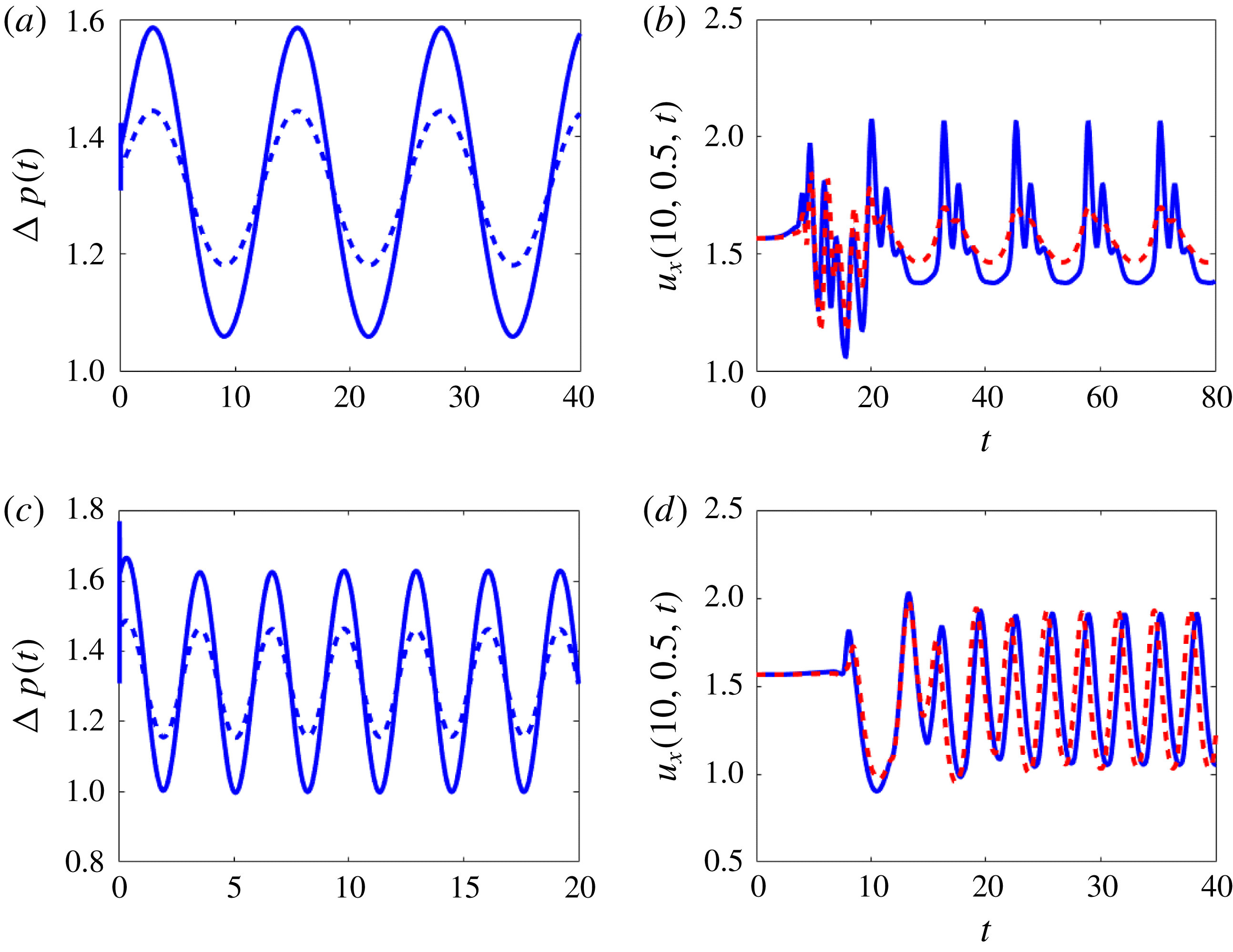
Figure 16 displays the time series of the pressure drop
 $\unicode[STIX]{x0394}p(t)$
(panels
 $a$
and
 $c$
) and the axial velocity at position
 $(x,r)=(10,0.5)$
, chosen to be in the region where roll-up occurs. Two values of the frequency and amplitude are chosen, namely
 $\unicode[STIX]{x1D6FA}=0.5;2$
and
 $\unicode[STIX]{x1D700}=0.1;0.05$
. The plots of the pressure drop show that this quantify is remarkably sinusoidal, even for the largest values of the amplitude. The oscillation levels for
 $\unicode[STIX]{x1D700}=0.1$
are approximately twice those for
 $\unicode[STIX]{x1D700}=0.05$
, confirming that the pressure drop is indeed proportional to the forcing. Remarkably, in all cases displayed, the pressure almost instantaneously stabilizes to a sinusoidal limit cycle, and a transient regime is almost unnoticeable, except for the very first time steps. The velocity signals show a rather different behaviour. For
 $\unicode[STIX]{x1D6FA}=0.5$
, the signal is very far from sinusoidal and displays a rich harmonic content. This confirms that the roll-up process occurring in this region is strongly nonlinear. The limit cycle at
 $x=10$
also takes time to establish, a fact associated with the time of convection of vortex structures. It is finally remarkable that the amplitude of oscillation for
 $\unicode[STIX]{x1D700}=0.1$
is not double compared to that for
 $\unicode[STIX]{x1D700}=0.05$
. This is also observed for
 $\unicode[STIX]{x1D6FA}=2$
, where the cases with
 $\unicode[STIX]{x1D700}=0.1$
and
 $\unicode[STIX]{x1D700}=0.05$
saturate to a limit cycle (closer to sinusoidal in this case) of same amplitude.
The pressure signal can be analysed in a finer way by decomposing into as a Fourier series in the form:
 $$\begin{eqnarray}\unicode[STIX]{x0394}p(t)=\unicode[STIX]{x0394}p_{0}+\mathop{\sum }_{j=1}^{\infty }\unicode[STIX]{x0394}p_{j}\sin (j\unicode[STIX]{x1D6FA}t-\unicode[STIX]{x1D719}_{j}).\end{eqnarray}$$
In practice, approximately 10 periods of oscillations were computed and the Fourier analysis was done after removing the first half of the time series, which is sufficient to discard the transient effect, as documented above. Figure 17 displays the discrete spectra, namely the absolute value of the amplitudes
 $|\unicode[STIX]{x0394}p_{j}|$
as a function of
 $j$
, extracted from all performed DNS. The
 $j=0$
component
 $\unicode[STIX]{x0394}p_{0}$
corresponds to the pressure drop associated with the mean flow, and is almost independent of
 $\unicode[STIX]{x1D700}$
. The
 $j=1$
component
 $\unicode[STIX]{x0394}p_{1}$
corresponds to the amplitude at the fundamental forcing frequency. This quantity is observed to be proportional to
 $\unicode[STIX]{x1D700}$
, confirming that the response to forcing is essentially linear. The components
 $\unicode[STIX]{x0394}p_{j}$
with
 $j>0$
correspond to the higher harmonics. These components are generally smaller than
 $10^{-4}$
, hence negligible. The case
 $\unicode[STIX]{x1D700}=10^{-1}$
leads to the largest values for the higher harmonics, but they still remain one order of magnitude smaller than the response at the driving frequency.
Discrete spectra of
 $\unicode[STIX]{x0394}p(t)$
for
 $\unicode[STIX]{x1D700}=10^{-1}$
(○),
 $\unicode[STIX]{x1D700}=10^{-2}$
(▫),
 $\unicode[STIX]{x1D700}=10^{-3}$
(♢),
 $\unicode[STIX]{x1D700}=10^{-4}$
(▿) and (a)
 $\unicode[STIX]{x1D6FA}=0.5$
, (b)
 $\unicode[STIX]{x1D6FA}=2$
and (c)
 $\unicode[STIX]{x1D6FA}=4$
.
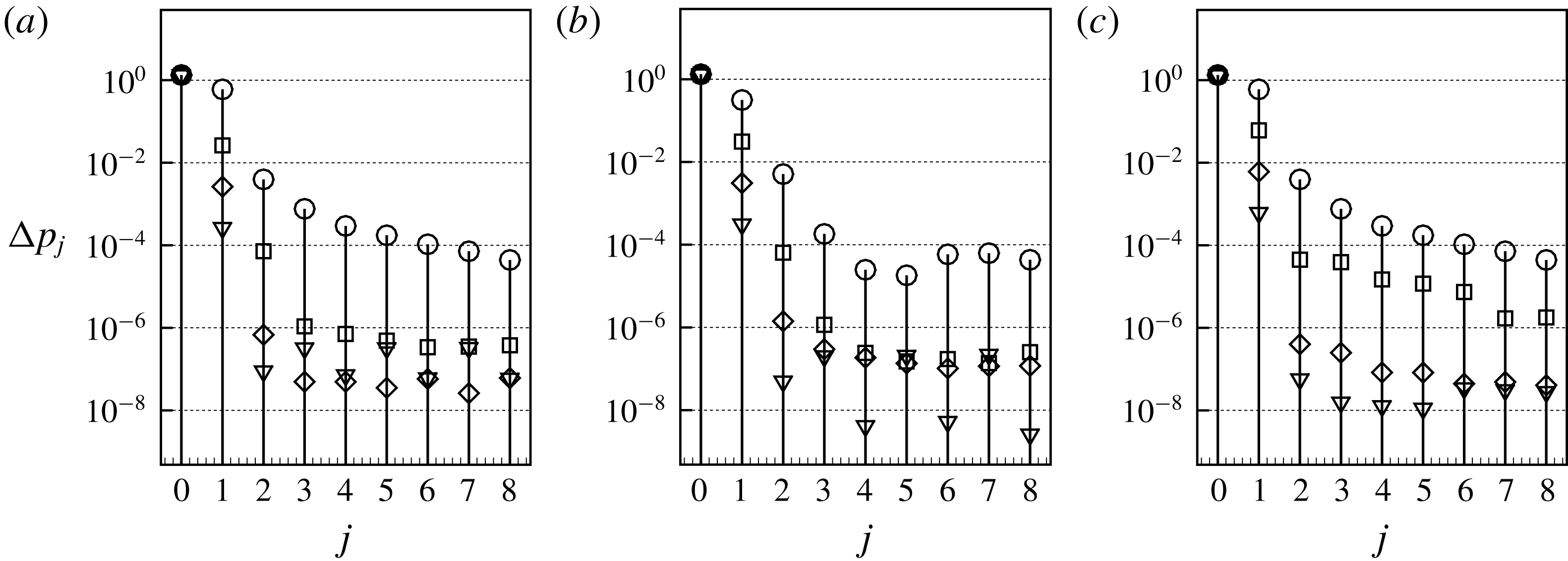
Truncating the Fourier series to the two first terms, i.e.
 $$\begin{eqnarray}\unicode[STIX]{x0394}p(t)\approx \unicode[STIX]{x0394}p_{0}+\unicode[STIX]{x0394}p_{1}\sin (\unicode[STIX]{x1D714}t-\unicode[STIX]{x1D719}_{1})\end{eqnarray}$$
and remembering that the flow rate can be written as
 $$\begin{eqnarray}q(t)=\underbrace{U_{in}\unicode[STIX]{x03C0}R_{in}^{2}}_{q_{0}}+\underbrace{U_{in}\unicode[STIX]{x03C0}R_{in}^{2}\unicode[STIX]{x1D700}}_{q_{1}}\sin (\unicode[STIX]{x1D714}t),\end{eqnarray}$$
we can calculate the impedance using only the first Fourier component of the pressure:
 $$\begin{eqnarray}\left.\begin{array}{@{}c@{}}\displaystyle Z_{R}=\unicode[STIX]{x0394}p_{1}/q_{1}\cos (\unicode[STIX]{x1D719}_{1}),\\ Z_{I}=\unicode[STIX]{x0394}p_{1}/q_{1}\sin (\unicode[STIX]{x1D719}_{1}).\end{array}\right\}\end{eqnarray}$$
Comparison between the DNS and the linear approximation in terms of pressure drop of the mean (base) flow and impedances.
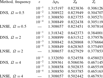
Table 2 displays the mean pressure drop
 $\unicode[STIX]{x0394}p_{0}$
and the impedance deduced from the DNS results for all cases simulated, and compares them to the LNSE results of §§ 4 and 5.
As for
 $\unicode[STIX]{x0394}p_{0}$
, the LNSE results displayed in the table actually correspond to the pressure drop associated with the base flow, namely the steady solution of the NSE, while the DNS results correspond to the mean flow obtained by time averaging. There is a subtle difference between these concepts (Barkley Reference Barkley2006), and the difference is expected to be of order
 $\unicode[STIX]{x1D700}^{2}$
. This is in agreement with the fact that deviations are only notable for the largest amplitude
 $\unicode[STIX]{x1D700}=10^{-1}$
.
As for the impedances, it is remarkable that the LNSE results provide an excellent approximation to the DNS results, with a relative error less than
 $1\,\%$
except for high frequency and large where it increases a little (we found the maximum relative error to be approximately
 $4\,\%$
at
 $\unicode[STIX]{x1D714}=4$
and
 $\unicode[STIX]{x1D700}=0.1$
).
7 Summary and discussion
The main goal of this study was to reconsider the classical problem of the response of an axisymmetric jet through a circular aperture through a plate of small thickness to harmonic forcing. This problem was initially considered by Howe who proposed an inviscid model which is still the basis of most studies of this problem. However a number of starting hypotheses of Howe’s model are questionable. In order to reconsider the problem on more rigorous grounds, our chosen approach has been to numerically solve the problem using the linearized Navier–Stokes equations (LNSE).
The first step of the LNSE approach consists of computing a base flow corresponding to the steady laminar flow through the aperture. Section 4 was devoted to the description of this base flow. Upstream of the aperture, it essentially consists of a radially convergent flow, while downstream of the aperture, the flow forms a quasi-parallel jet bounded by a thin vorticity layer originating from the rim. As classically observed in experiments, the radius of the jet is smaller than the radius of the aperture. We documented this effect in terms of the vena contracta coefficient
 $\unicode[STIX]{x1D6FC}$
. Our numerical results indicate an almost constant value
 $\unicode[STIX]{x1D6FC}\approx 0.61$
in the range
 $10^{3}<Re<10^{4}$
, in agreement with classical experiments.
The second step of the LNSE approach consists of solving a linear problem for small-amplitude disturbances with harmonic temporal dependence. A standard implementation of this method, starting from a formulation in terms of physical coordinates
 $(x,r)$
on a numerical domain ‘large enough’ to resolve correctly the structure of the linear perturbation (typically
 $[r_{max},x_{max}]=[20,80]$
), was first tried. This first implementation was found to lead to difficulties in the high Reynolds number range, leading to the impossibility of obtaining reliable results as soon as
 $Re\gtrsim 1000$
. These difficulties were analysed, and the problem was found to be linked to the strong spatial amplification properties of the jet. To overcome these difficulties, a convenient method was designed, which consists of reformulating the problems in terms of a mapped complex coordinate
 $X(x)$
. The idea of using complex coordinates is not new in linear acoustics, and is at the basis of the perfectly matched layer (PLM) method to prevent reflections of the acoustic waves on the boundaries of the domain. However, to our knowledge, the use of such a method in strictly incompressible problems is new. We show that an appropriate choice of the mapping function allows us to get rid of the spatial amplification of the perturbation in the axial, mapped direction.
Although the spatial structure of the perturbation no longer has a physical interpretation when computed using complex coordinates, we demonstrated that the global quantities depending only on the pressure jump across the hole, such as the vena contracta coefficient and the impedances, are well resolved. This method thus allows us to obtain meaningful results using a much smaller numerical domain (typically
 $[R_{max},L_{out}]=[15,15]$
) and incidentally a much lighter numerical grid.
Using this method, we then characterized the response of the jet to harmonic forcing by computing its impedance, namely the ratio between the fluctuating pressure jump and fluctuating flow rate across the aperture, which is a key quantity used by acousticians to characterize the interaction of jet flows with acoustic fields. In all cases the real part of the impedance was found to be positive, meaning that exciting the jet at a given frequency necessitates the provision of energy from an outer system. Moreover, the impedance was found to become independent of the precise value of
 $Re$
as soon as
 $Re\gtrsim 1500$
, indicating the existence of a high Reynolds number asymptotic regime.
Results in this high Reynolds number regime were compared to predictions of Howe’s model. The comparison was done in terms of the Rayleigh conductivity, which is a concept directly related to the impedance and used by a fraction of the acoustic community as an alternative. Comparison shows substantial deviations, especially in the range of intermediate non-dimensional frequencies, indicating that some of the hypotheses underlying Howe’s model are too restrictive.
Finally, to confirm the validity of our linearized approach, we also performed direct numerical simulations considering harmonic perturbations with small but finite amplitude
 $\unicode[STIX]{x1D700}$
. The spatial structure of the perturbations computed in this way showed a rapid saturation of the spatial instability towards an array of vortex rings, very different from the structure computed using LNSE. Despite this, the values of the impedance extracted from these DNS, as well as the properties of the mean flow, were found to be in excellent agreement with LNSE results, with a maximum relative error of only a few per cent for
 $\unicode[STIX]{x1D700}=0.1$
. This result confirms that the LNSE is an efficient method to predict the impedance, even in cases where the spatial evolution of the perturbations is rapidly dominated by nonlinear effects.
We end this discussion with a few closing remarks. First, coming back to the complex mapping technique used in the LNSE approach, we stress that this method was designed to overcome a mathematical difficulty linked to the linear problem, namely strong spatial amplification extending very far away in the axial direction. As such, this method is not suited to a direct numerical solution in the nonlinear regime, and the DNS presented in § 6 were thus performed in physical coordinates. On the other hand, the method is potentially usable for studying the linear stability of large class of flows characterized by nearly parallel spatially unstable regions, such as the wakes of blunt or profiled bodies. We are currently investigating the applicability of complex mapping for such problems.
Secondly, since our whole approach relies on an assumed laminar base flow, one may question the applicability of our results when considering turbulent jets. Although the precise threshold is difficult to predict, transition to turbulence in such jets is typically thought to take place in the range
 $Re\in [10^{3}-10^{4}]$
. However, when transition takes place, turbulence is only observed in the downstream region located after the near-field vena contracta region which remains essentially laminar. Having observed in our DNS that the nonlinear evolution of vortex structures in the far field does not affect the value of the impedance, we can postulate that the same is true regarding nonlinear effects due to turbulence, and thus that our results, obtained under the hypothesis of a laminar flow, are actually applicable to turbulent jets in a large range of parameters.
Third, in the whole study, we have only considered axisymmetric disturbances to the flow. Non-axisymmetric disturbances also exist in such flows, and in high Reynolds number jets their signature has been detected among turbulent structures (Sasaki et al. Reference Sasaki, Piantanida, Cavalieri and Jordan2017). However, such non-axisymmetric disturbances are not associated with a net flow rate through the hole. So, they are expected to be much less coupled to acoustic disturbances, and indeed it is not possible to describe them in terms of an impedance.
Finally, we have mentioned in the introduction that in the case where the thickness of the plate is not small compared to the radius of the hole, the jet can cease to act as a sound damper to become a sound generator, leading to the possibility of self-sustained oscillations of the jet. In such a case, the impedance concept is a useful tool to characterize the instability mechanism, and the numerical method designed in the present paper is directly applicable to investigation of such instabilities. A parametric study of the response of jets through plates of finite thickness to harmonic forcing is underway and will be presented in a forthcoming paper.
Appendix A. Inviscid stability analysis of a cylindrical vortex sheet
In this appendix we review the stability analysis of a cylindrical vortex sheet, a classical problem first addressed by Batchelor & Gill (Reference Batchelor and Gill1962).
A.1 Equations
We consider as a base flow a cylindrical jet with a top-hat profile, with radius
 $R_{J}$
and velocity
 $U_{J}$
:
 $$\begin{eqnarray}U_{x}(r)=\left\{\begin{array}{@{}ll@{}}U_{J} & \text{if }r<R_{J};\\ 0 & \text{if }r>R_{J}.\end{array}\right.\end{eqnarray}$$
This corresponds to a cylindrical shear layer. The stability analysis of this flow can be studied by adding small perturbations in potential form, both inside (
 $\unicode[STIX]{x1D719}_{o}$
) and outside (
 $\unicode[STIX]{x1D719}_{i}$
) the jet. These perturbations are searched in eigenmode form as follows:
 $$\begin{eqnarray}\unicode[STIX]{x1D719}_{i}=AI_{m}(kr)\text{e}^{\text{i}(kx-\unicode[STIX]{x1D714}t)};\quad \unicode[STIX]{x1D719}_{o}=BK_{m}(kr)\text{e}^{\text{i}(kx-\unicode[STIX]{x1D714}t)};\quad \unicode[STIX]{x1D702}=C\text{e}^{\text{i}(kx-\unicode[STIX]{x1D714}t)},\end{eqnarray}$$
where
 $r=R_{J}+\unicode[STIX]{x1D702}$
is the location of the jet edge.
The matching conditions at
 $r=R$
are continuity of the pressure (
 $p_{i}=p_{o}$
), and kinematical conditions connecting the temporal derivative of
 $\unicode[STIX]{x1D702}$
to the radial velocity
 $\unicode[STIX]{x2202}\unicode[STIX]{x1D719}/\unicode[STIX]{x2202}r$
. Hence:
 $$\begin{eqnarray}\displaystyle & \displaystyle \text{i}(\unicode[STIX]{x1D714}-kU_{J})\unicode[STIX]{x1D719}_{i}(R_{J})=\text{i}\unicode[STIX]{x1D714}\unicode[STIX]{x1D719}_{o}(R_{J}), & \displaystyle\end{eqnarray}$$
 $$\begin{eqnarray}\displaystyle & \displaystyle -\text{i}\unicode[STIX]{x1D714}\unicode[STIX]{x1D702}=(\unicode[STIX]{x2202}\unicode[STIX]{x1D719}_{o}/\unicode[STIX]{x2202}r)_{r=R_{J}}, & \displaystyle\end{eqnarray}$$
 $$\begin{eqnarray}\displaystyle & \displaystyle \text{i}(kU_{J}-\unicode[STIX]{x1D714})\unicode[STIX]{x1D702}=(\unicode[STIX]{x2202}\unicode[STIX]{x1D719}_{i}/\unicode[STIX]{x2202}r)_{r=R_{J}}. & \displaystyle\end{eqnarray}$$
Eliminating constants
 $A,B,C$
, we get the following dispersion relation:
 $$\begin{eqnarray}D(\unicode[STIX]{x1D714},k)=(\unicode[STIX]{x1D714}-kU_{J})^{2}+L_{0}(kR_{J})\unicode[STIX]{x1D714}^{2}=0,\end{eqnarray}$$
where
 $$\begin{eqnarray}L_{0}(k)=-\frac{I_{0}^{\prime }(kR_{J})K_{0}(kR_{J})}{I_{0}(kR_{J})K_{0}^{\prime }(kR_{J})}.\end{eqnarray}$$
Note that this dispersion relation generalizes the classical one for Kelvin–Helmholtz instability of an infinitely thin shear layer (obtained by replacing
 $L_{0}(k)$
by one). In the short-wavelength range (
 $kR_{J}\gg 1$
),
 $L_{0}$
is close to one and the problem is effectively equivalent to the planar shear layer. On the other hand, in the long-wavelength range (
 $kR_{J}\gg 1$
),
 $L_{0}$
tends to zero leading to different trends.
A.2 Temporal stability analysis
In a temporal stability framework (
 $k\in \mathbb{R}$
), the dispersion relation leads to:
 $$\begin{eqnarray}c=\frac{\unicode[STIX]{x1D714}}{k}=U_{J}\frac{1\pm \text{i}\sqrt{L_{0}}}{1+L_{0}},\end{eqnarray}$$
where
 $c=c_{r}+\text{i}c_{i}$
is the phase velocity. The real part of the phase velocity represents the convection velocity of the disturbance, which corresponds to the term noted
 $U_{c}$
in Howe’s model. In the short-wave range,
 $L_{0}\approx 1$
leading to
 $c_{r}=U_{J}/2$
, which is the classical result for a planar shear layer. On the other hand, in the long-wave range, the asymptotic trends becomes
 $c_{r}\approx U_{J}$
.
A.3 Spatial stability analysis
In a spatial stability framework, which is more relevant here,
 $\unicode[STIX]{x1D714}\in \mathbb{R}$
and the problem has to be solved for the complex eigenvalue
 $k$
. The dispersion relation has no analytical solution but is easily solved numerically. Results are reported in figure 18. The spatial amplification rate
 $-k_{i}$
and the real part of the wavenumber
 $k_{r}$
(related to the wavelength) are both increasing functions of
 $\unicode[STIX]{x1D714}$
. In the spatial framework one can still define the convection velocity of perturbations as
 $c_{r}=Re(\unicode[STIX]{x1D714}/k)$
. This quantity is plotted in the figure with a thick line. We observe that the spatial analysis essentially leads to the same conclusion, namely the convection velocity of perturbations is close to
 $U_{J}/2$
in the high-frequency (i.e. short-wavelength) regime and close to
 $U_{J}$
in the low-frequency (i.e. long-wavelength) regime.
Spatial stability analysis of a top-hat jet: – –,
 $k_{r}$
;
 $\cdots \,$
,
 $-k_{i}$
; ——,
 $c_{r}=Re(\unicode[STIX]{x1D714}/k)$
.
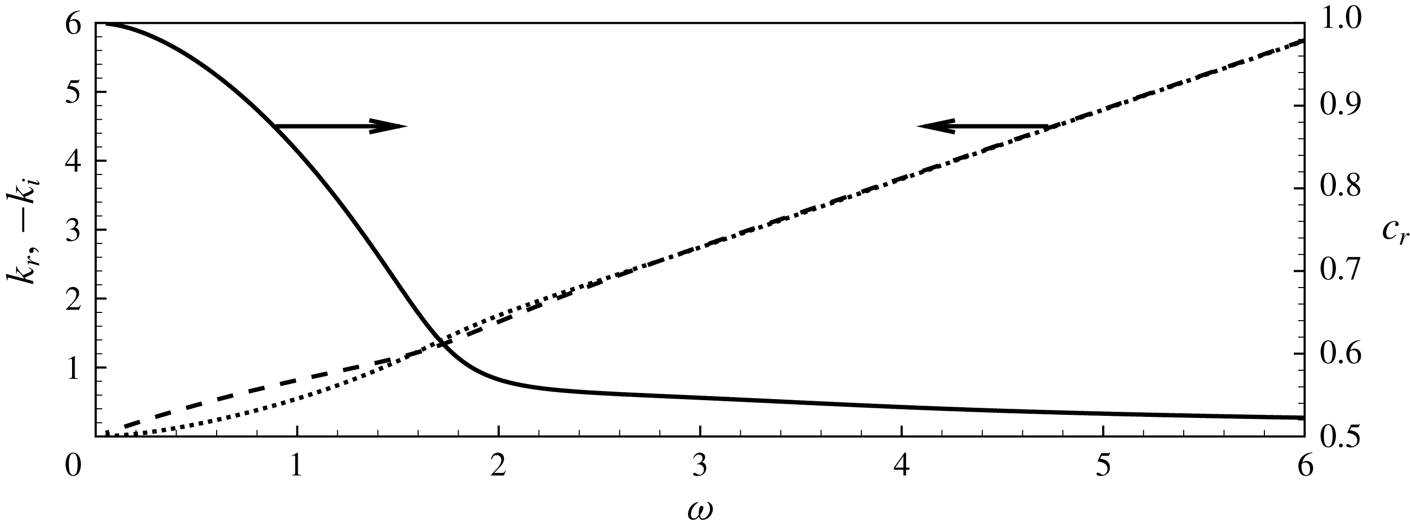
Appendix B. Numerical validations
In this appendix, we provide additional results obtained by varying the defining the mesh dimensions, grid density as well as the parameters defining the complex mapping function. All meshes used in the study are described in table 3. Meshes
 $\mathbb{M}_{0}$
and
 $\mathbb{M}_{1}$
are the reference meshes used in the paper, respectively without and with the use of complex mapping. Meshes
 $\mathbb{M}_{2-7}$
are additional meshes using complex mapping, with different choices for the dimensions, parameters and/or density. Meshes
 $\mathbb{M}_{8-9}$
are additional meshes without complex mapping, with different dimensions in the axial direction.
B.1 Complex mapping validation
We first provide a few additional results to illustrate the failure of the resolution in physical coordinates to compute the impedance for large Reynolds numbers, and the efficiency of the complex mapping technique to resolve it.
Comparison between the results of impedances obtained using the complex coordinate mapping (—♢—, mesh
 $\mathbb{M}_{1}$
) and without mapping with
 $L_{out}=40R_{h}$
(—○—, mesh
 $\mathbb{M}_{8}$
) and
 $L_{out}=80R_{h}$
(—▫—, mesh
 $\mathbb{M}_{0}$
) at
 $Re=500$
.
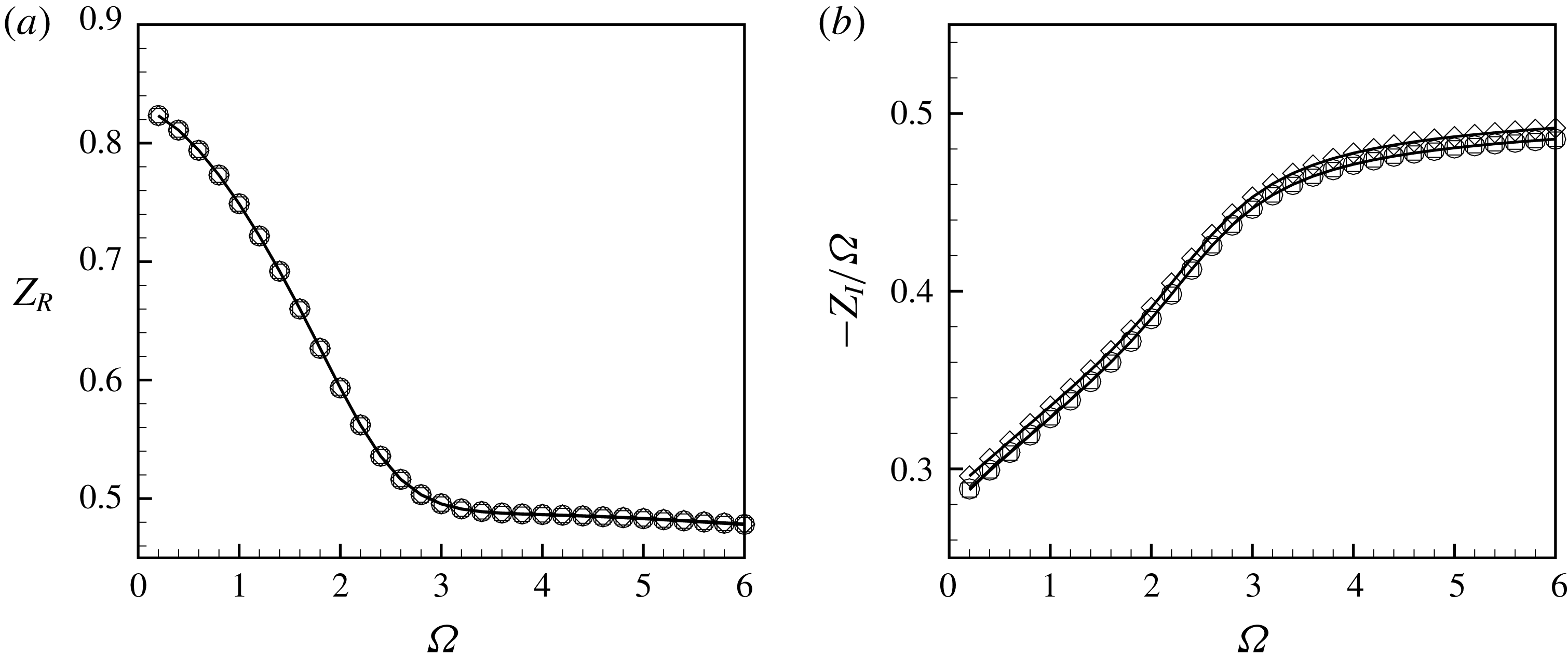
Description of numerical meshes
 $\mathbb{M}_{0{-}9}$
in term of dimensions, mapping parameters and number of triangles
 $n_{t}$
.
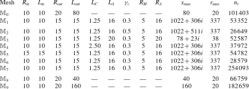
Impedances computed using the complex coordinate mapping (—♢—, mesh
 $\mathbb{M}_{1}$
) and without mapping with
 $L_{out}=80R_{h}$
(—○—, mesh
 $\mathbb{M}_{0}$
) and
 $L_{out}=160R_{h}$
(—▫—, mesh
 $\mathbb{M}_{9}$
) at
 $Re=2000$
.
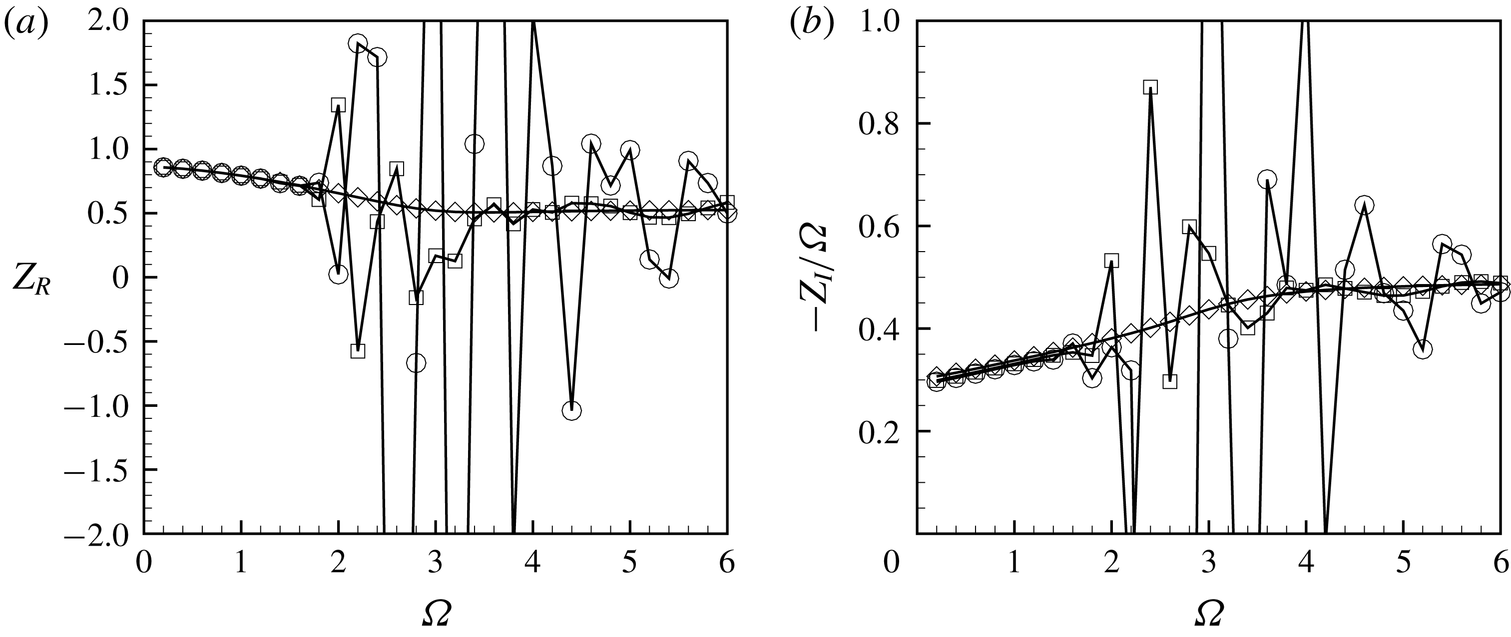
Figure 19 displays a comparison between the impedances for
 $Re=500$
calculated using the reference meshes as well as an additional mesh
 $\mathbb{M}_{8}$
designed without complex mapping and a with a shorter axial dimension. As one can observe, in this range of Reynolds number, results obtained with and without complex mapping are almost identical: the curves are perfectly overlapped for
 $Z_{R}$
whereas for
 $Z_{I}$
a little difference exists but with relative errors less than
 $1\,\%$
.
Figure 20 present a similar comparison for
 $Re=2000$
, using this time an additional mesh without complex mapping of longer axial dimension (mesh
 $\mathbb{M}_{9}$
with
 $L_{out}=160R_{h}$
). From the figure, it is clear that the computation of the impedance without the mapping is impossible. The reference mesh
 $\mathbb{M}_{0}$
leads to non-physical oscillations in the range
 $\unicode[STIX]{x1D6FA}\gtrsim 2$
. Doubling the size of the domain does not lead to notable improvements, and the use of complex mapping proves to be the only way to obtain reliable results.
Pressure perturbation on the symmetry axis for
 $Re=2000$
and
 $\unicode[STIX]{x1D6FA}=3$
computed with complex mapping (mesh
 $\mathbb{M}_{1}$
; ——) and without complex mapping (mesh
 $\mathbb{M}_{9}$
with
 $L_{out}=160R_{h}$
; – –).
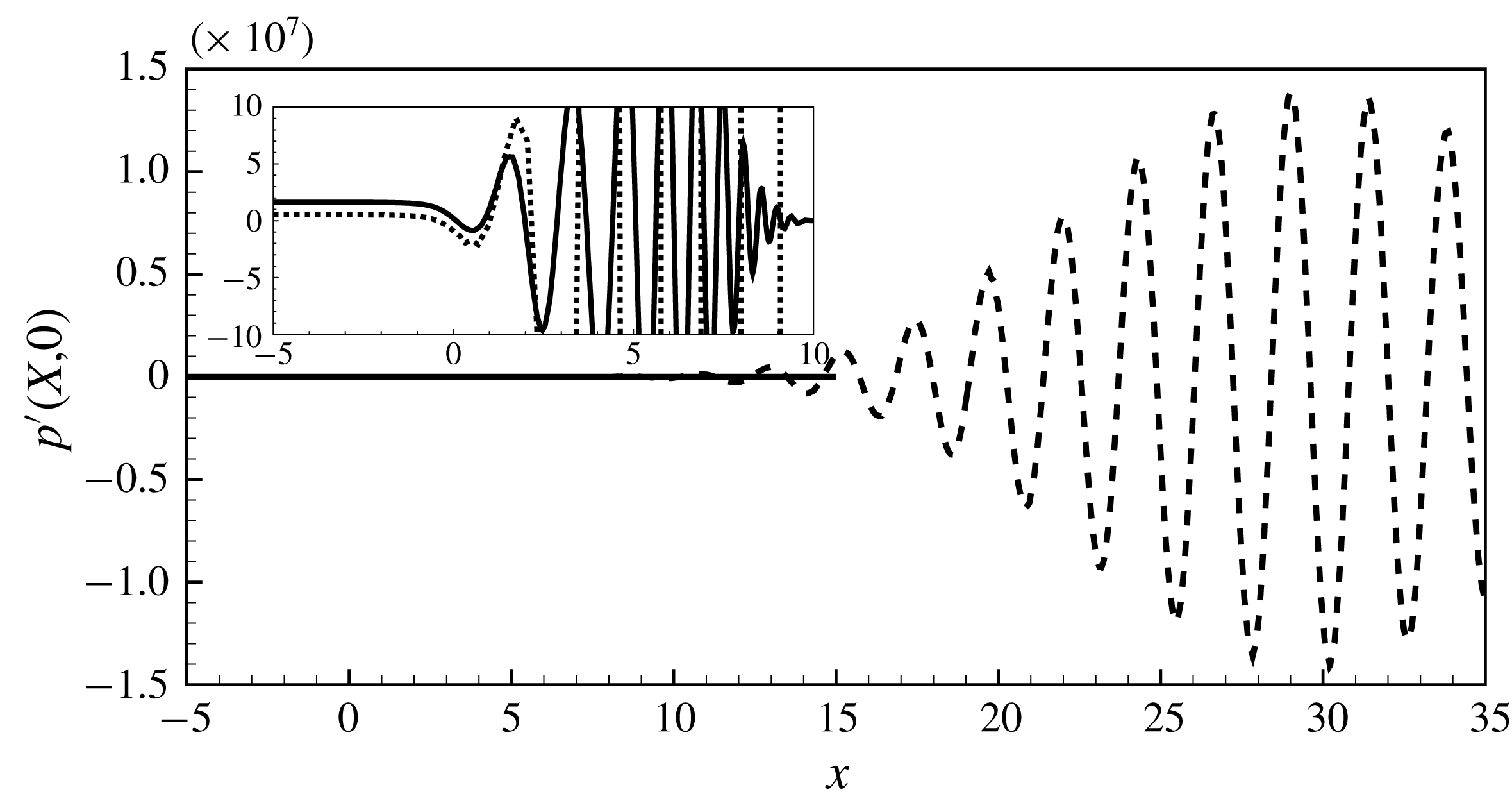
To illustrate further the failure of the numerical resolution without complex mapping, we report in figure 21 the pressure of the perturbation on the symmetry axis for
 $Re=2000$
and
 $\unicode[STIX]{x1D6FA}=3$
. As can be seen, the amplitudes in physical coordinates reach levels of order
 $10^{7}$
. As a consequence, round-off errors can occur, leading to an error propagation in all the domain and so a wrong pressure level at inlet. This is visible in the inset displaying a zoom in of the inlet region, showing a mismatch between the results with and without complex mapping.
B.2 Robustness of the complex mapping
In order to validate the mapping and to verify its robustness, we performed a sensitivity analysis of the impedances to geometrical and mapping parameters variation.
(a) Real part and (b) imaginary part of the impedance at
 $\text{Re}=3000$
computed with the mesh
 $\mathbb{M}_{1}$
(—▫—),
 $\mathbb{M}_{2}$
(—▵—),
 $\mathbb{M}_{3}$
(—▿—),
 $\mathbb{M}_{4}$
(—♢—) and
 $\mathbb{M}_{5}$
(—○—).
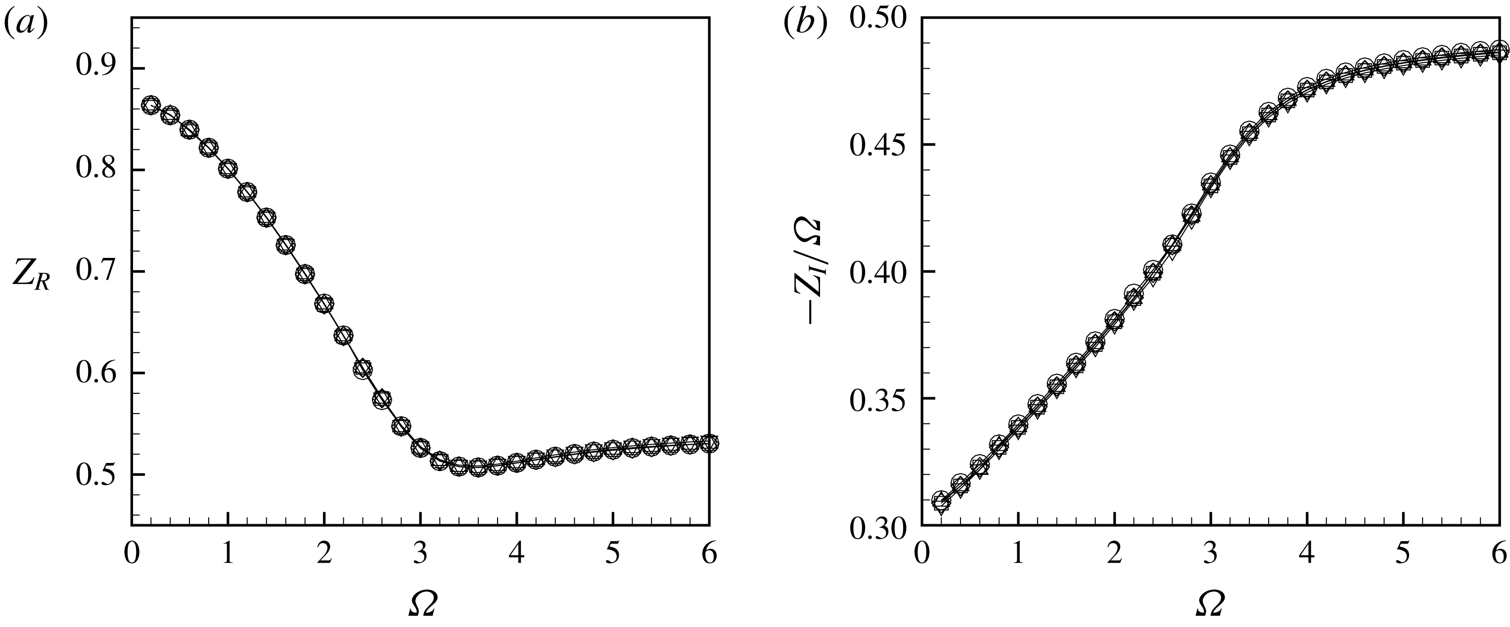
In figure 22 we compare the impedances for at
 $Re=3000$
, computed with meshes
 $\mathbb{M}_{1-5}$
. One can observe that the curves are all overlaid on the reference curves, namely the mesh
 $\mathbb{M}_{1}$
used to calculate the impedances in § 5.3, showing the robustness and the efficiency of the mapping formula used.
Finally, the last numerical issue is about the thickness of the hole. In the whole paper we assume a zero-thickness hole, but to generate the mesh we had to specify a small but finite value. We set it to
 $10^{-4}$
and we verified that results were insensitive to this length.
(a) Real part and (b) imaginary part of the impedance at
 $\text{Re}=3000$
computed with the mesh
 $\mathbb{M}_{1}$
(—▫—),
 $\mathbb{M}_{6}$
(—○—) and
 $\mathbb{M}_{7}$
(—♢—).
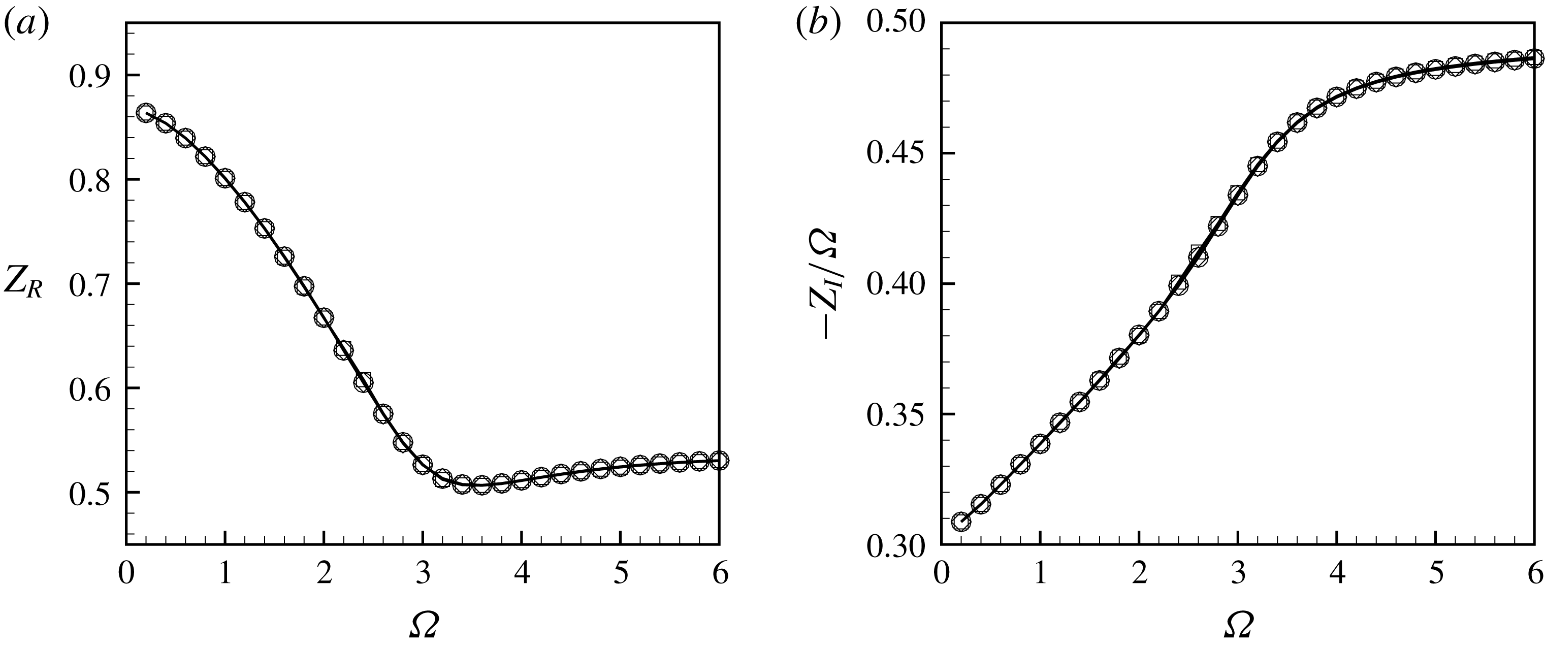
Relative error calculated on the absolute value of the impedance between the meshes
 $\mathbb{M}_{6}-\mathbb{M}_{7}$
(– –♢– –) and the meshes
 $\mathbb{M}_{1}-\mathbb{M}_{7}$
(—○—) at
 $Re=3000$
.
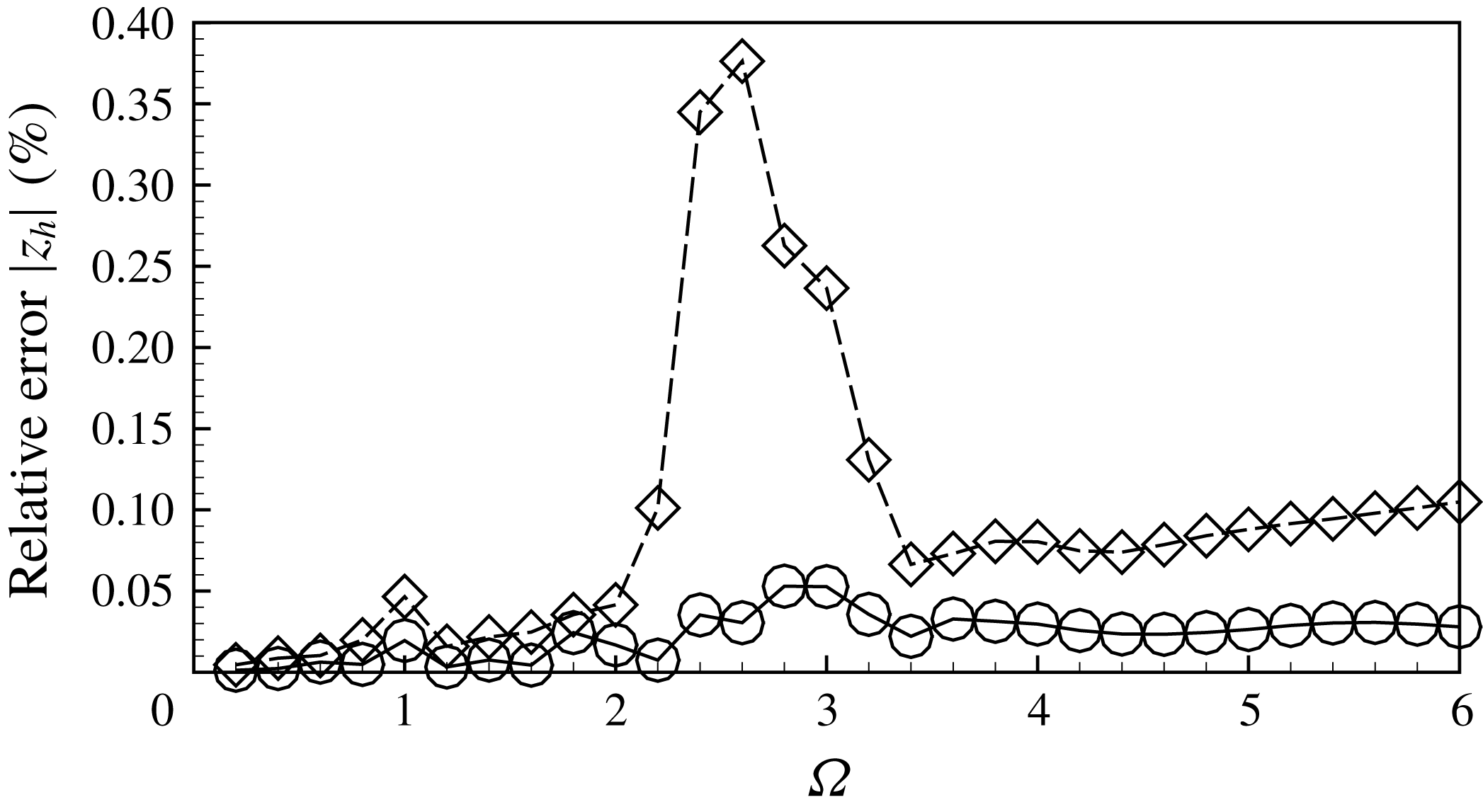
B.3 Mesh convergence
The last issue to consider for numerical validation is the sensitivity of the results to the grid density. As explained in § 3, the mesh generation process involves mesh adaptation thanks to the adaptmesh command of the FreeFem++ software. Although the procedure is automatic, its efficiency can be tuned by specifying an interpolation error parameter. Mesh
 $\mathbb{M}_{1}$
was obtained using the default value
 $5\times 10^{-3}$
. Two additional meshes were designed, respectively with interpolation errors of
 $10^{-2}$
(mesh
 $\mathbb{M}_{6}$
) and
 $10^{-3}$
(mesh
 $\mathbb{M}_{7}$
). Table 4 gives the number of triangles
 $n_{t}$
of each of these meshes, as well as the corresponding number of degrees of freedom (
 $n_{d.o.f}$
) of the finite element discretization. In the last two columns of the table, we report the values obtained for the vena contracta coefficient for
 $Re=500$
and
 $Re=2000$
with each of these meshes. One can observe that results are accurate up to the fourth digit. In figure 23 we compare the impedances computed with each of these meshes for
 $Re=3000$
. The figure shows that the curves are completely overlapped. We also quantified the relative error of the meshes
 $\mathbb{M}_{1}$
and
 $\mathbb{M}_{6}$
with respect to
 $\mathbb{M}_{7}$
for all the frequencies. From figure 24 we can observe that the maximum relative error committed using the mesh
 $\mathbb{M}_{6}$
is around
 $0.38\,\%$
, whereas the maximum error is reduced to
 $0.005\,\%$
using the mesh
 $\mathbb{M}_{1}$
.
Characteristic of the meshes used for the convergence analysis using the mapping parameters reported in table 3 and convergence of the base flow. Note that
 $n_{d.o.f.}$
is the number of degrees of freedom of the mesh.

B.4 Numerical efficiency
One of the advantages of using LNSE compared to full DNS is that the first approach only requires resolution of a small number of linear problems, while the second one requires time integration of the equations over a long time covering several periods of oscillation to ensure convergence. In this section we demonstrate the numerical efficiency of the method by indicating in table 5 the CPU time required for the various steps of the analysis. As can be seen, the amount of time to obtain an impedance curve
 $Z(\unicode[STIX]{x1D6FA})$
in the range
 $\unicode[STIX]{x1D6FA}\in [0-6]$
(including generation of the base flow and adapted mesh, and resolution of elementary problems for 100 values of
 $\unicode[STIX]{x1D6FA}$
spanning the range) on a standard computer is of the order of 15 min using resolution in real coordinates, and can be reduced to as small as 6 min using the complex mapping method.
As a comparison, using the DNS time stepping we have used for generating the results displayed in § 6, using
 $\mathbb{M}_{0}$
, a time step
 $\text{d}t=2\times 10^{-3}$
and performing 40 000 time steps to cover several oscillation periods required a total CPU time of approximately 15 h, for a single value of the parameters
 $\unicode[STIX]{x1D6FA}$
and
 $\unicode[STIX]{x1D716}$
.
CPU time on a standard computer (MacBook Pro 2012, 2.5 GHz Intel Core
 $i5$
, 4 Gb RAM) required for computation of a base flow and generation of an adapted mesh following the procedure explained in § 4, resolution of a linear problem for a single value of
 $\unicode[STIX]{x1D6FA}$
and full parametric study of the impedance, including generation of base flow and mesh, and resolution of 100 linear problems in the range
 $\unicode[STIX]{x1D6FA}\in [0-6]$
.

Appendix C. The complex base flow
As mentioned in § 3 and detailed in appendix B, as soon as
 $Re>1500$
, converged results for the impedance can only be obtained using the complex mapping technique. In the present implementation of the method, we chose to compute the base flow in the same coordinates. In this appendix we briefly document the structure of the base flow when computed in this way.
Real (upper part) and imaginary (lower part) of the axial velocity
 $U_{x}$
of the base flow at
 $Re=3000$
.
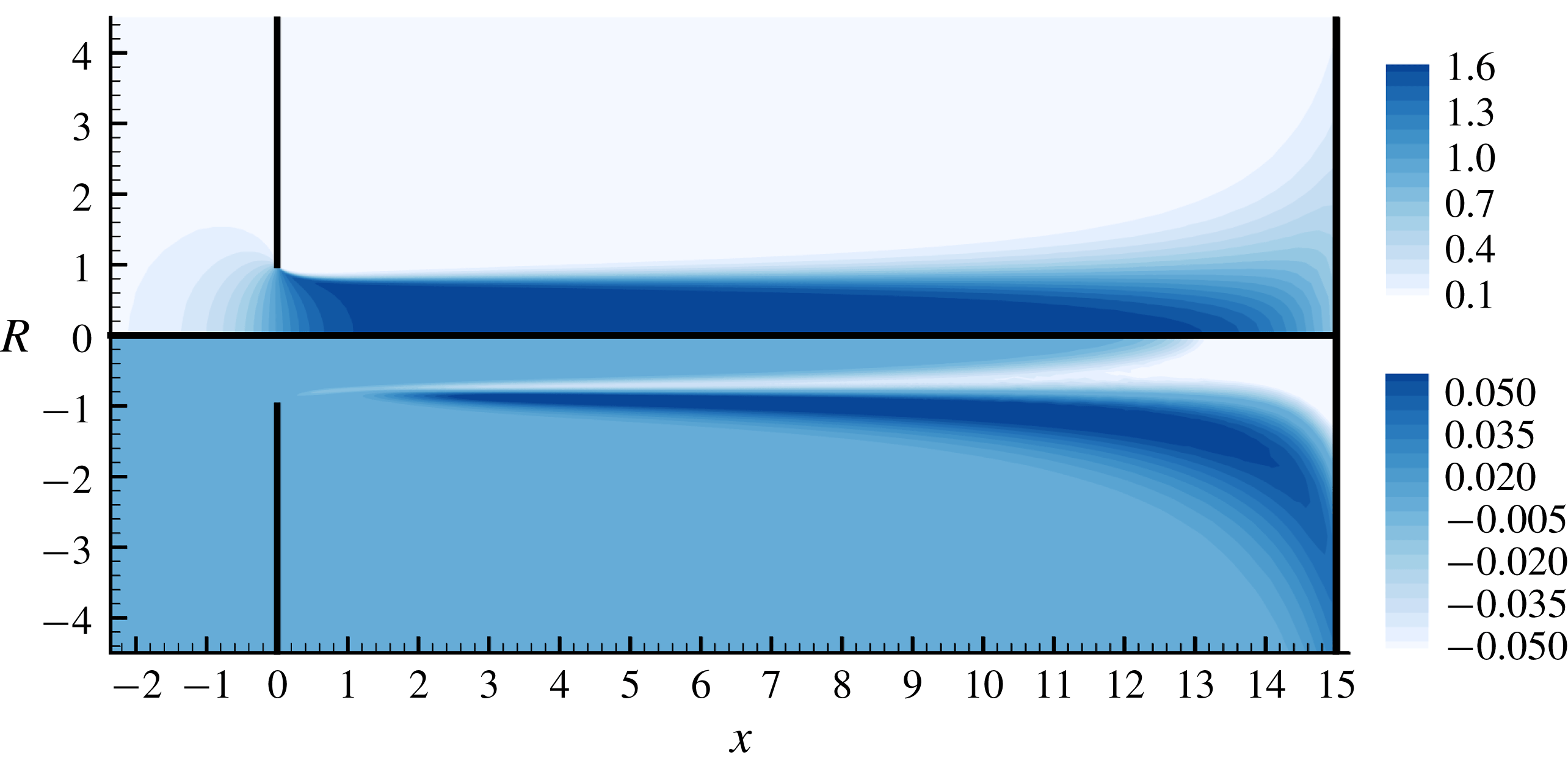
Figure 25 displays the axial velocity component of the base flow
 $U_{x}$
obtained in this way. This quantity is actually the analytical continuation of the axial velocity (displayed in figure 4) in the complex
 $x$
-plane. The real part (upper plot) has a structure similar to the one in real coordinates plotted in figure 4, but one can observe that the thin shear layer rapidly enlarges as one progresses along the
 $X$
direction. This is mostly an effect of the stretching involved in the coordinate mapping: the computation is made with
 $L_{out}=15$
and
 $L_{A}=16$
, so that the position in the
 $X$
direction corresponding to
 $|x|\rightarrow \infty$
is actually just a little outside of the computational domain.
The lower part displays the imaginary part of
 $U_{x}$
. Here the complex coordinate mapping is done with
 $L_{C}=1.25$
, so the imaginary part becomes significant above this value in the
 $X$
direction.



