This article offers forecasts made on July 22, 2010, for the 2010 state legislative elections. Most work in the election forecasting field has been done on presidential and U.S. House elections. Less has been done for U.S. Senate elections, and almost none for gubernatorial or state legislative elections. This year will see much attention directed at the 43 state legislatures holding elections, because many will have the responsibility for drawing new district lines based on the 2010 census. Furthermore, of those chambers with elections scheduled in 2010, seven currently contain one party with less than a 5% margin of control. With so much at stake, these will clearly be contests to watch.
The forecasts based on the following analysis predict that the Republicans will gain control of 11 legislative chambers, leaving them with a total of 46 of 98 partisan chambers.Footnote 1
MODELING STATE LEGISLATIVE ELECTIONS
Underlying the model used here is research showing partisanship to be stable for many voters, therefore making the strength of a party in a given area relative to other areas similar from one election to the next. Voters who are less attached to a particular party tend to reward the incumbent party for good times and punish them for bad. Furthermore, these swing voters prefer policy moderation in government and vote to promote this preference. These theoretical considerations are reflected in the independent variables used in the model, described in the following sections.
The unit of analysis of the statistical model on which the forecasts were based was the state legislative election, yielding a total of 75,693 cases. Data between 1968 and 2008 from 48 states were included in the analysis, with Nebraska, Louisiana, and, for some years, Minnesota excluded.Footnote 2 Uncontested elections were not examined, since these can be called in advance. The dependent variable in the analysis was the percentage of the two-party vote received by the Democrats, and state legislative election data were drawn from Carsey et al. (Reference Carsey, Niemi, Berry, Powell and Snyder2008a; Reference Carsey, Niemi, Berry, Powell and Snyder2008b).Footnote 3
Whenever possible, independent variables matching those in Klarner's Reference Klarner2008 forecasts were used. Four categories of independent variables were used: district characteristics, candidate characteristics, national-level factors, and state-level factors. District characteristics were measured by the percent of the two-party vote that the Democrats received in a district's last state legislative election, with 0 or 100 put into the appropriate uncontested elections. Presidential vote returns at the state legislative level were not available. A variable was coded 1 for seats that were Democratic and uncontested in the prior election, −1 for seats that were Republican and uncontested, and 0 for other cases. This variable was labeled “Contestation Advantaget−1,” for reasons that will be provided. The coefficient of this variable was hypothesized to be negative in sign, because a district with an uncontested election in the last period was not assumed to be equivalent to a district in which one party won all the votes. The presence of free-for-all multi-member districts (FFA MMDs) necessitated adjustment of this variable for such districts. An FFA MMD might have been undercontested in a prior election. For example, only two Democrats might have run in a district with three seats, which would hurt their electoral prospects. This adjustment involved finding a fraction that divided the number of Democratic candidates by the number of seats and subtracting it by a second fraction derived for Republican candidates.
When redistricting had altered districts since the last election, district- and candidate-level variables were coded as missing and imputed with Gary King's Amelia program (King et al. Reference King, Honaker, Joseph and Scheve2001; Honaker et al. Reference Honaker, Joseph, King, Scheve and Singh2001). Numerous sources including Hardy, Heslop, and Anderson (Reference Hardy, Heslop and Anderson1981); Hardy, Heslop, and Blair (Reference Hardy, Heslop and Blair1993); and Weber (Reference Weber1995; Reference Weber and Governments2005) were consulted to determine when redistricting occurred.Footnote 4 Had I assumed that new legislative districts only came into effect in the first election in a district after a decennial census, 7.5% of cases would have been miscoded.
Although uncontested elections were excluded from the analysis, undercontested elections in FFA MMDs were not. The variable “Contestation Advantage” was measured in the same way as the lagged variable described previously, except in the current period, to capture the advantage that contestation would give a party.
For single-member districts (SMDs),Footnote 5 a variable was coded 1 for an election with a Democratic incumbent, −1 for an election with a Republican incumbent, and 0 for other cases to capture the well-known tendency for incumbents to achieve a greater share of the vote (Jacobson Reference Jacobson2004). For FFA MMDs, the incumbency variable consisted of one fraction, determined by the number of Democratic candidates who were incumbents divided by the number of seats in the FFA MMD, minus a second fraction, determined by the number of Republican candidates who were incumbents divided by the number of seats in the FFA MMD. Furthermore, I included a variable that measured whether a seat had been vacated because of state legislative term limits. This variable was coded 1 if the seat was held by the Democrats in the prior election, −1 if it was held by the Republicans, and 0 in other cases. For FFA MMDs, the variable had an analogous adjustment to the other candidate-level variables. This variable's coefficient was expected to be positive, because some of the incumbency effect was hypothesized to be caused by the retirement of incumbents with dim electoral prospects (Engstrom and Monroe Reference Engstrom and Monroe2006). A dummy variable coded 1 was included when a chamber had any incumbents facing term limits.
Berry, Berkman, and Schneiderman (Reference Berry, Berkman and Schneiderman2000) found that incumbents did better in state legislatures that had more funding than incumbents in legislatures for which funding was lower. Legislative budgets include such items as legislator salaries, postage and brochures, staff salaries, other staff expenses, travel allowances, and other items that may aid reelection. Accordingly, biennial funding for the legislature, per legislator, deflated by the revised 2009 version of the Berry-Fording-Hanson (Berry, Fording, and Hanson Reference Berry, Fording and Hanson2000) state cost-of-living index, was included in the model and interacted with the incumbency variable (measured in thousands of 2007 dollars), the measure used by Berry, Berkman, and Schneiderman (Reference Berry, Berkman and Schneiderman2000).Footnote 6
A variable that measured the prior elective experience of non-incumbents was not available. However, whether a state senate candidate was a former state lower house member was included in the model. This variable, labeled “Former State House Member” was coded 1 when such a candidate was a Democrat, −1 when such a candidate was a Republican, and 0 in other cases. The variable was adjusted in an analogous way to those previously described for FFA MMDs. A dummy variable indicating whether an election was a state senate election was also included.
I hypothesized that the decision mechanisms that voters use in elections at the national level influence their votes for state legislators. According to this belief, as the public approves more of the president's performance or the state of the national economy, the more they reward the president's “team.” In this model, presidential approval was measured by the percent of people who approved of the job performance of the president in the Gallup survey closest to 123 days before the election, which was July 1 in 2010. That figure was multiplied by −1 in the case of a Republican president, which necessitated the inclusion of a dummy variable coded 1 when the president was a Democrat. The strength of the economy was measured by percentage change in real personal income between the first quarters of the years prior to and of the election, and this figure was multiplied by −1 during a Republican presidency. Changes in real personal income were theorized to be the best overall summary of economic health (Bartels and Zaller Reference Bartels and Zaller2001). Furthermore, I posited that voters are more likely to vote against legislators of the president's party in presidential midterm years to moderate policy. A variable labeled “National Midterm Penalty” was coded 1 in midterm election years with a Democratic president, −1 in Republican midterm years, and 0 in other years. Although most state legislative elections occurred in even numbered years, the presence of 3,128 odd-year elections appreciably increased the information available to assess the impact of national-level factors by doubling the number of years analyzed.Footnote 7
State-level analogues to the national-level factors were included in the model whenever possible. Unfortunately, the availability of gubernatorial approval data was limited, so that variable was not included in the analysis. However, measures for a number of other state-level factors were available. The state economy was measured as described previously, but at the state level, and deflated by the state cost-of-living indicator already described. Percent change in real income growth across the states in 2010 displayed notable differences, and taking state cost-of-living into account markedly altered the ranking of states' economic health. This variable was multiplied by −1 when the governor was Republican and by 1 when the governor was a Democrat.Footnote 8 A state-level midterm penalty variable was also included (Bailey and Fullmer Reference Bailey and Fullmer2008). For state elections with four-year gubernatorial terms, the variable was coded 1 during Democratic governors' terms, −1 during Republican governors' terms, and 0 during gubernatorial election years.
For all independent variables, a lagged component was also included. Lagged variables of all independent variables are necessary to capture time-series dynamics (De Boef and Keele Reference De Boef and Keele2008). For example, say there are two districts in which the Democrats received 65% of the vote, but one district had a Democratic incumbent while the other did not. All else being equal, the latter district would be more Democratic in its voting disposition. Failing to control for lagged incumbency would therefore distort the meaning of the lagged dependent variable. Here, lagged independent variables were expected to have the opposite sign as their nonlagged components. As reported in the following, when the nonlagged component was statistically significant, the lagged component was statistically significant with the opposite sign five out of seven times.
The existence of FFA MMDs necessitated a second round of analysis. For example, say that an FFA MMD had three seats and three candidates from each major party. If the Democrats received 55% of the vote, they would win either two or three seats. In the elections examined here, 36% of FFA MMDs saw split delegations, when at least one Democrat and one Republican were elected from the same district. Secondary models converting votes into seats at the district level were therefore constructed (not shown), the results of which were used in the Monte Carlo analysis described later.
Multi-level modeling was used, with level-3 error terms for years and level-2 error terms for state-years. Likelihood ratio tests found that the inclusion of the level-2 and/or level-3 error terms were necessary (p < .0000). Not taking year or state-year level error terms into account would have biased and shrunk the Monte Carlo-produced forecast confidence intervals described in the following section (Klarner Reference Klarner2008).
RESULTS
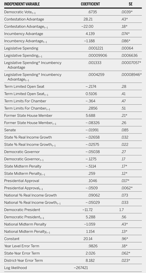
Many of the factors that were posited to have an association with Democratic success in state legislative elections were found to do so. Table 1 displays the results of the analysis. Unless noted, all nonlagged variables' coefficients were statistically significant and showed the expected signs. The prior Democratic share of the vote was associated with the current vote, and the negative coefficient associated with “Contestation Advantaget−1” indicated that a prior uncontested election was not equivalent to 100% of the vote for that party. Incumbents received larger percentages of the vote than non-incumbents, and the interaction term between incumbency and legislative spending indicated that the incumbency effect was greater in better-funded legislatures. The lagged variable that measured the interaction between incumbency and legislative spending had a positive sign, contrary to expectations. This unexpected outcome may mean that the impact of prior spending carried over to the next election. The variable measuring open seats caused by term limits was not found to be associated with candidates' success. Taken as a whole, these findings indicate that the resources of office, and not strategic retirements, account for the incumbency effect. Senate challengers who were former members of their states' lower houses did substantially better than candidates who had not been members of a lower house. Such challengers received 5.7% more of the vote.
Determinants of State Legislative Election Outcomes, 1968–2008

Note. The dependent variable is the Democratic percent of the two-party vote. *p < .05, one-tailed test.
The variable “State Midterm Penalty” indicated that legislators who shared the party of the governor lost about 0.4% of the vote. No evidence was found to indicate that the health of the state economy influenced state legislative elections. National factors did surprisingly well in the model. An increase of 1% in presidential approval or real national income growth was associated with a 0.10% and 0.09%, respectively, increase in votes for legislators of the president's party. Although the observed impact of presidential approval was probably not due to chance (p < .05), the state of the national economy failed to achieve statistical significance. These effects were similar in magnitude to those found for the U.S. House by Klarner (Reference Klarner2008). Last, state legislative candidates of the president's party were found to receive about 1% fewer votes than candidates from the out-party, an impact greater than that found for the state midterm penalty.
A final test computed the model for the years 1968 to 2006 and made forecasts for the 2008 elections in the same manner as for the 2010 elections described later. Results are not shown, as they were substantively the same as those shown in table 1. Predictions for individual-level races were made and a Monte Carlo analysis was conducted to compute the probability that a particular chamber would be won by the Democrats. Random variables were generated two thousand times to reflect the three different levels of error terms, as well as the uncertainty associated with the independent variables' coefficients (Beck Reference Beck, Campbell and Garand2000). Predictions at the district level were aggregated to the chamber and added to the number of seats the Democrats held in the uncontested elections, as well as to the seats not up for election. Control of the chamber was called two thousand times on the basis of these simulations.
At the district level, the predictions were reasonably accurate, although biased in a Democratic direction. The average two-party Democratic predicted vote for the 3,015 contested elections of 2008 was 52.1%, but the estimates averaged 55.6%. When the actual percentage of the Democratic vote was regressed on the predicted percentage, the resulting standard error of the estimate was 7.85 (8.04 for SMDs only). For SMDs, 89.0% of contested races were called correctly (2,486 out of 2,793), and 93.8% of SMDs were called correctly when uncontested elections (there were 2,133 uncontested SMDs) were included.Footnote 9
When 3.5% was added to all Republicans' vote percentages, accuracy only improved slightly. Additionally, forecast errors were not larger or smaller by state in a statistically significant sense. Table 1 reports a much larger district-level (level-1) error term than did the level-2 and level-3 error term estimates. These findings indicate that noise at the district level was by far the largest source of error and may well be caused by the absence of presidential vote returns in the model.
Of the 84 chambers up for election, seven were called incorrectly, including one that ended up with tied control (91.7% correct). However, this split chamber should be reclassified as correct, because the direction of change was correctly predicted, making the percent correctly predicted 92.9%. Seven chambers switched party control as a result of the elections (not including two that became split and one that was previously split), and four of these were called correctly by the model. However, if the three chambers that involved splits are considered, seven switches out of 10 were correctly called. The model accurately predicted that the Alaska state senate would be split, giving this outcome a 37.7% chance, a greater predicted probability than the 35.3% chance of Republican control or the 27.0% chance of Democratic control. For the other two splits, the direction of change was correctly forecast. The model also predicted 10 switches of party control, meaning there were only three false positives. One standard with which to judge how well the model performed is to compare it against a “naïve model,” which predicts that party control will not switch. That model had an 88.1% correct forecast, reducing forecast error by two-fifths (11.9% to 7.1%) with the model used here.
FORECASTS
This article makes forecasts for 5,271 districts in 81 chambers in 43 states.Footnote 10 By July 15, 2010, 22 states had held their primaries, enabling candidate characteristics to be coded for 2,570 districts (48.8%). Furthermore, by this date, filing deadlines had passed in all but two states, which allowed me to code candidate characteristics of many races with certainty. In an additional 930 races (17.6% of the 5,271 districts), no candidates had filed for one major party's primary, which allowed the race to be called for the other party. Another 1,541 districts (29.2%) had either no incumbent among the filers or an incumbent unchallenged in the primary, which allowed incumbency to be coded. This left 4.3% of races in which an incumbent (or incumbents) was being challenged and the general election would be contested.
The Monte Carlo analysis was conducted once with these 4.3% of races coded in as pro-Democratic of a direction as possible regarding incumbency, and once with pro-Republican codes. The 41 cases in which there was uncertainty about whether a former house member would run in a contested general senate election were dealt with in the same way. In most cases, these low and high estimates did not differ markedly, but one exception is noted below.
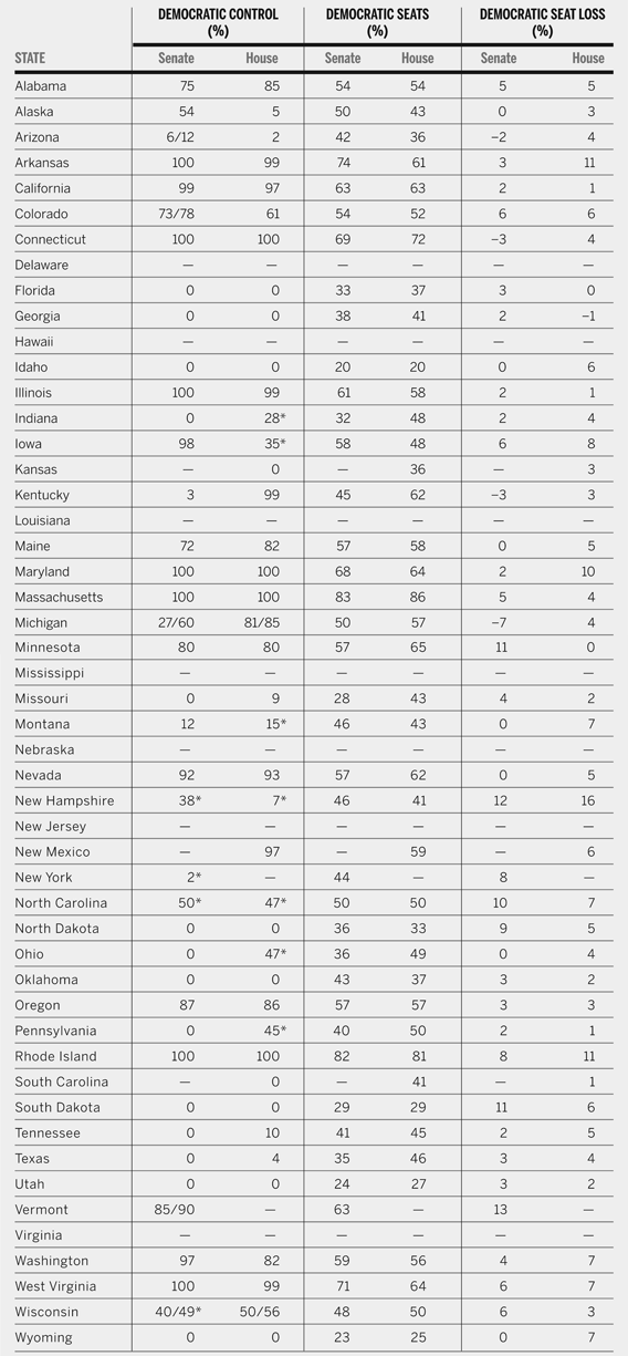
Table 2 reports the percent probability that the Democrats will control a given chamber after the election.Footnote 11 Forecasts of the percentage of seats held by the Democrats are also reported in the table, as well as the change in that percent in a pro-Republican direction.Footnote 12 Asterisks denote a predicted switch in party control. The model predicted that the Republicans would take control of 11 state legislative chambers, including the Indiana, Iowa, Montana, New Hampshire, North Carolina, Ohio, and Pennsylvania houses, and the New Hampshire, New York, North Carolina, and Wisconsin senates. The model predicted a 54% chance that the Alaska senate will stay split.Footnote 13
Forecast Chance of Democratic Control by State Legislative Chamber, 2010

* = a predicted switch in party control. Cells with two percentages represent a low and high predicted probability that the chamber will be won by the Democrats.
Differences in pro-Democratic and pro-Republican estimates of the probability of Democratic control were below 5% for all but five chambers. The Michigan senate had a 31% chance of Democratic control with pro-Republican codes, and a 67% chance of Democratic control with pro-Democratic codes. This instability was caused by 29 out of 38 districts that had term-limited incumbents. The resulting large field of primary candidates included many former house members, who may win or lose these contests. This outcome highlighted the importance of the primaries for party control. The Michigan senate Democrats were predicted to increase their seats by 7% in a Republican year. Why? Seventeen of the term-limited incumbents are Republicans.
Table 2 also indicates that several chambers that will have the primary responsibility for redistricting appreciable numbers of U.S. House districts will be fiercely contested, with between 28% and 61% probability of Democratic control. These states include Colorado, Indiana, Iowa, Michigan, North Carolina, Ohio, Pennsylvania, and Wisconsin, with a total of 115 U.S. House seats.Footnote 14 For state legislative elections, the Midwest is shaping up to be a battleground.