Quantification of added-mass effects using particle image velocimetry data for a translating and rotating flat plate

S. J. Corkery; H. Babinsky; W. R. Graham

doi:10.1017/jfm.2019.231

Quantification of added-mass effects using particle image velocimetry data for a translating and rotating flat plate

Published online by Cambridge University Press: 10 May 2019

and

S. J. Corkery*: Affiliation:
Department of Engineering, University of Cambridge, Cambridge CB2 1PZ, UK
H. Babinsky: Affiliation:
Department of Engineering, University of Cambridge, Cambridge CB2 1PZ, UK
W. R. Graham: Affiliation:
Department of Engineering, University of Cambridge, Cambridge CB2 1PZ, UK
*: †Email address for correspondence: sjc276@cam.ac.uk

Article contents

Abstract
Introduction
Theoretical description of the vortex sheets
Quantification of $\unicode[STIX]{x1D6FE}^{b}$ from particle image velocimetry
Description of the experiments
Results
Lost circulation compensation
Conclusion
References

Rights & Permissions

Abstract

Added mass characterises the additional force required to accelerate a body when immersed in an ideal fluid. It originates from an asymmetric change to the surrounding pressure field so the fluid velocity satisfies the no-through-flow condition. This is intrinsically linked with the production of boundary vorticity. A body in potential flow may be represented by an inviscid vortex sheet and added-mass forces determined using impulse methods. However, most fluids are not inviscid. It has been theorised that viscosity causes the ‘added-mass vorticity’ to form in an intensely concentrated boundary layer region, equivalent to the inviscid distribution. Experimentally this is difficult to confirm due to limited measurement resolution and the presence of additional boundary layer vorticity, some the result of induced velocities from free vorticity in the flow field. The aim of this paper is to propose a methodology to isolate the added-mass vorticity experimentally with particle image velocimetry, and confirm that it agrees with potential flow theory even in separated flows. Experiments on a flat-plate wing undergoing linear and angular acceleration show close agreement between the theoretical and measured added-mass vorticity distributions. This is demonstrated to be independent of changes to flow topology due to flow separation. Flow field impulse and net force are also consistent with theory. This paper provides missing experimental evidence coupling added mass and the production of boundary layer vorticity, as well as confirmation that inviscid unsteady flow theory describes the added-mass effect correctly even in well-developed viscous flows.

JFM classification

Low-Reynolds-number flows: Low-Reynolds-number flows Vortex Flows: Vortex Flows

Information

Type: JFM Papers
Information: Journal of Fluid Mechanics , Volume 870 , 10 July 2019, pp. 492 - 518
DOI: https://doi.org/10.1017/jfm.2019.231 [Opens in a new window]
Copyright: © 2019 Cambridge University Press

1 Introduction

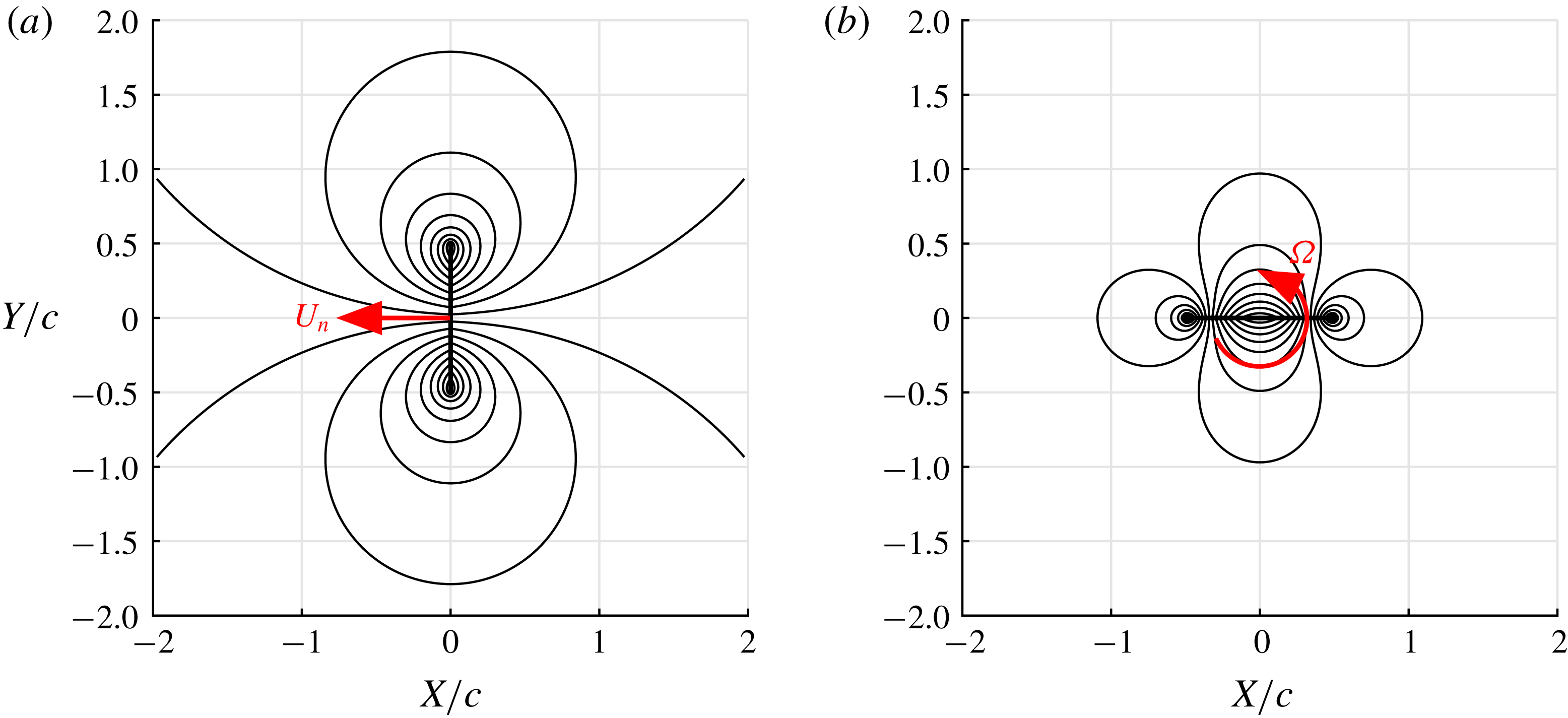
Added or virtual mass is an unsteady fluid dynamic effect that has been discussed in the literature for over a century (refer to Lamb Reference Lamb1895; Darwin Reference Darwin1953; Brennen Reference Brennen1982; Benjamin Reference Benjamin1986; Saffman Reference Saffman1992). It describes an increase in the force required to accelerate a body at a given rate when immersed in a fluid compared to the equivalent kinematics in a vacuum. While the mass of the body is unchanged whether surrounded by fluid (or not), Darwin (Reference Darwin1953) showed that a physical volume of fluid is ‘carried’ by a body during its motion in potential flow. This is the so-called ‘drift volume’, the mass of which corresponds to the added mass. Take, for example, an infinitely thin two-dimensional flat plate in an inviscid, incompressible and irrotational fluid. If the fluid and plate are both initially at rest, and the plate is accelerated in either a translational or angular manner, then the surrounding fluid must also accelerate to accommodate the changing velocity of the plate. This gives rise to the flow fields shown in figure 1. The acceleration is actioned by pressure waves that propagate from the plate surface, at infinite speed for an incompressible fluid. A difference in surface pressures across the thickness of the plate generates a net force (or moment) on the plate. The flow field experiences a net change in momentum to match the impulse (in the classical mechanics sense) applied to the plate; equivalently the kinetic energy of the flow is changed to match the work done. The additional force required to accelerate the plate is proportional to the rate of linear or angular acceleration. For the translating plate shown in figure 1(a), the proportionality constant (added mass) is equal to the mass per unit length of a cylindrical volume of fluid with a diameter equal to the chord.

Figure 1.

Streamlines for a flat plate with chord length $c$ in potential flow: (a) translation with velocity $U_{n}$ ; (b) rotation with angular velocity $\unicode[STIX]{x1D6FA}$ about the mid-chord. Streamlines are shown for the moving-body reference frame.

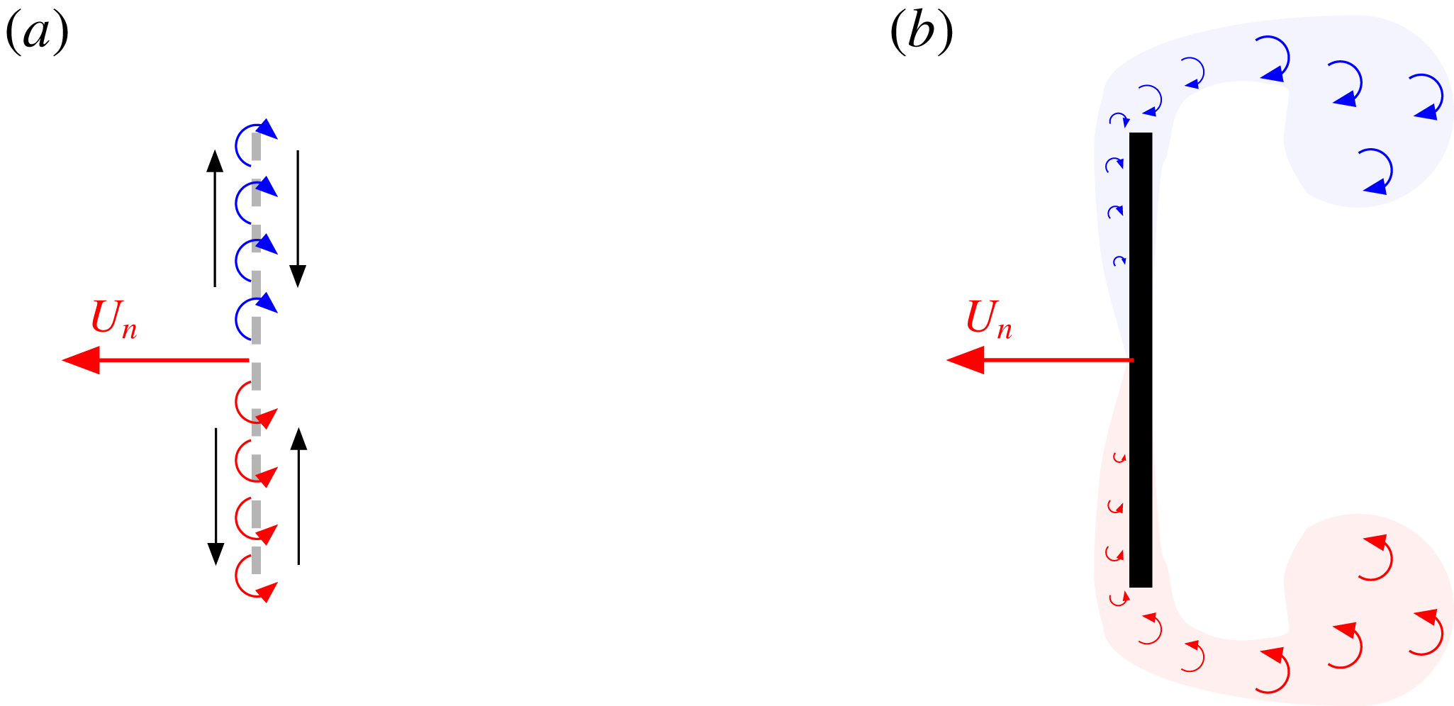
An alternative representation of the added-mass effect can be made by considering flow field vorticity. In potential flow theory, a body may be represented by an inviscid and infinitely thin vortex sheet on its surface, in an otherwise irrotational flow (Saffman Reference Saffman1992). As illustrated in figure 2(a) for the case of a translating plate, the strength of the vortex sheet is given by the discontinuous ‘slip’ in velocity either side of the plate. By application of the Biot–Savart law, the velocity of the flow field, momentum and force can be determined uniquely by this distribution of vorticity. The resulting impulse-derived force (see Wu (Reference Wu1981) or appendix A) is identical to the added-mass force obtained directly from the pressure field.

For applications of practical interest, however, the working fluid is not inviscid and, as shown in figure 2(b), the flow field can be significantly different from that of potential flow. Diffusion causes vorticity to be transmitted from the surface of a body into the adjacent fluid. When subjected to a strong adverse pressure gradient, such as that about sharp edges, the resulting boundary layer can separate. Vorticity is thus shed into the bulk flow, giving a rotational, non-potential, field. An additional problem arises when applying the inviscid interpretation for added mass to a viscous flow field. The no-slip condition means that the aforementioned surface slip velocity cannot occur; rather, when a body accelerates, vorticity must diffuse into the lower region of the boundary layer. Leonard & Roshko (Reference Leonard and Roshko2001) and Eldredge (Reference Eldredge2010) have argued that the added-mass force on a body is proportional to the rate at which new vorticity is generated on the body surface, with an identical singular distribution to that given by inviscid theory. This is regardless of viscous effects and consequential changes to flow topology. Graham, Pitt Ford & Babinsky (Reference Graham, Pitt Ford and Babinsky2017) assumed a similar process to identify the added-mass contribution to the forces derived from experimental data. This ‘added-mass vorticity’ diffuses from the surface and into the surrounding flow over time periods of the order of the Reynolds number, greater than the convective time scale. In practice, it is therefore confined to an intensely spatially concentrated region.

Figure 2.

Schematic comparing vorticity distributions between potential flow (a) and a viscous flow field (b). In the viscous fluid, vorticity is diffused and advected from the plate surface, whereas vorticity is contained in an infinitely thin layer for the inviscid fluid. Red and blue colours correspond to positive and negative vorticity, respectively.

This leads to the motivation behind the present work. While the existence of the added-mass vorticity has been theorised, there are no experimental flow field measurements confirming its presence and demonstrating its independence of the bulk rotational flow. The wealth of measurements taken in the literature utilising particle image velocimetry (PIV) to resolve the flow field around an accelerating body, such as that about pitching, plunging or rotating aerofoils, have spatial resolutions of the order of a boundary layer thickness (see Poelma, Dickson & Dickinson Reference Poelma, Dickson and Dickinson2006; Rival, Prangemeier & Tropea Reference Rival, Prangemeier and Tropea2009; Buchner et al. Reference Buchner, Buchmann, Kilany, Atkinson and Soria2012; Pitt Ford & Babinsky Reference Pitt Ford and Babinsky2013; Polet, Rival & Weymouth Reference Polet, Rival and Weymouth2015). The intention of such investigations is to capture wide regions of the flow field, including starting vortices, which reduces spatial resolution. It is questionable whether with such measurements the distribution of added-mass attributed vorticity can be resolved and isolated from changes made to the flow field resulting from other viscous effects.

In this paper a methodology to isolate the added-mass vorticity experimentally (with PIV) is proposed. Measurements are taken for a flat-plate wing undergoing translation and rotation. These test cases are used because any planar kinematics may be decomposed into a combination of such motions. From the resulting data the added-mass attributed component of vorticity, located within the boundary layer, is quantified. This is compared with the vortex sheet predicted using potential flow theory to demonstrate that the potential solution is valid, even for cases with significant flow separation. Using the measures of added-mass attributed vorticity, flow field impulse and force on the plate are calculated. These are also compared with the potential flow solutions for a plate undergoing comparable kinematic motion, thereby investigating the effect of PIV resolution on the determination of impulse and force quantities. The work therefore further develops understanding of unsteady incompressible flows, the limitations of a common measurement technique, and may inform future reduced-order models of such flows.

2 Theoretical description of the vortex sheets

A potential flow model is used to determine the ‘theoretical’ added-mass vortex sheet, as well as the sheet attributable to velocities induced on the plate from vorticity in the bulk flow field. The approach is based on the work of Graham et al. (Reference Graham, Pitt Ford and Babinsky2017), who derived these quantities for a flat-plate wing translating with constant angle of incidence. In this work the method is extended to incorporate rotation about the mid-chord.

2.1 Problem geometry

Figure 3.

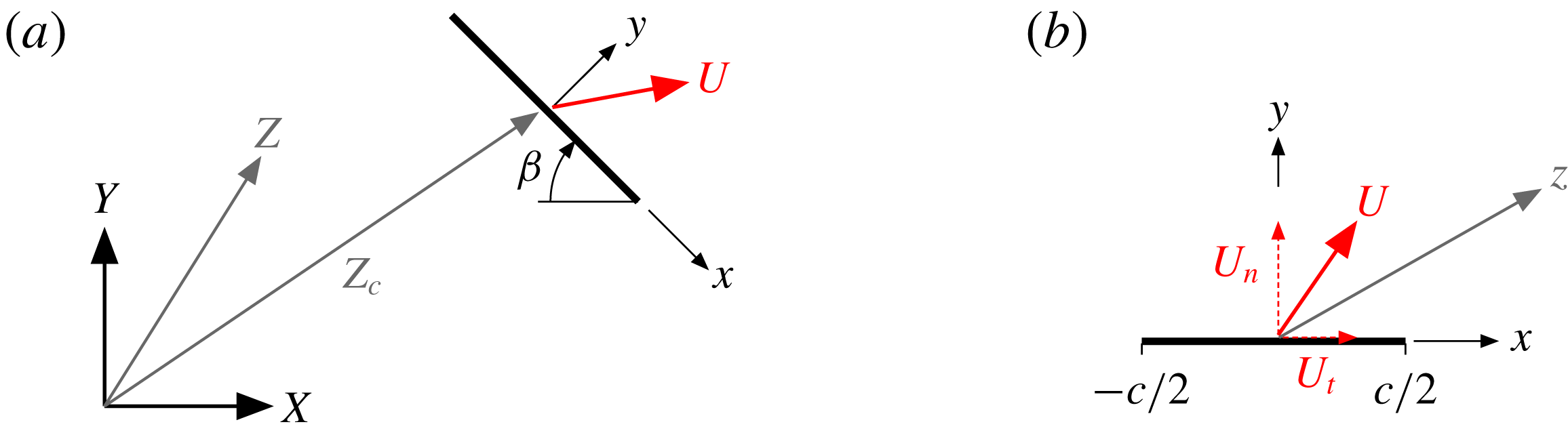
Problem geometry and coordinates frames: (a) global ‘fixed’ coordinate frame and (b) plate frame.

The geometry of the problem is shown in figure 3. The flow field is assumed to be unbounded and at rest at an infinite distance from the globally ‘fixed’ $XY$ coordinate system origin. Positions in the flow field are given in complex vector notation $Z=X+\text{i}Y$ . The plate, with chord length $c$ , has the position $Z_{c}=X_{c}+\text{i}Y_{c}$ defined at the mid-chord and complex velocity $U=\text{d}Z_{c}/\text{d}t$ . For many calculations it is simpler to work in a plate reference frame $xy$ . As shown in figure 3(b), this is centred at the mid-chord with $x$ in the plate tangential direction and $y$ in the plate-normal direction, oriented at an angle $\unicode[STIX]{x1D6FD}$ to the $XY$ coordinate frame. Positions in the flow field relative to the plate frame are given by the complex position $z=x+\text{i}y$ , related to the global frame by

(2.1)

$$\begin{eqnarray}z=\text{e}^{\text{i}\unicode[STIX]{x1D6FD}}(Z-Z_{c}).\end{eqnarray}$$

The plate velocity vector $U$ can be resolved into a component normal to the plate $U_{n}$ ( $y$ direction) and a tangential component $U_{t}$ ( $x$ direction). Only the plate-normal velocity $U_{n}$ is of importance, as the tangential component does not contribute to the velocity difference across the plate. The angular velocity of the plate is $\unicode[STIX]{x1D6FA}=-\text{d}\unicode[STIX]{x1D6FD}/\text{d}t$ .

2.2 Vortex sheet

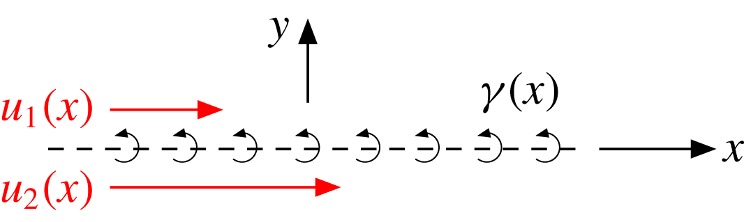
In inviscid flow about an infinitely thin flat plate, there is generally a discontinuity in surface flow velocity across the plate. As defined by (2.2) and illustrated in figure 4, the difference in this surface ‘slip’ velocity is equivalent to a vortex sheet. In this context the vortex sheet represents the vorticity contained by boundary layers either side of the plate. For a real flow boundary layer, vorticity is spread across a finite thickness, but as the viscosity of the fluid reduces to zero, the vorticity becomes confined to an infinitely thin layer. Eldredge (Reference Eldredge2010) and Graham et al. (Reference Graham, Pitt Ford and Babinsky2017) argued that the vortex sheet has two constituent parts as given by (2.3). The first, $\unicode[STIX]{x1D6FE}^{nc}$ , is attributed to body motion in an otherwise irrotational flow. This is the vortex sheet associated with added mass. It has the defining characteristic of zero net circulation and is given the superscript $nc$ for ‘non-circulatory’. The second constituent part, $\unicode[STIX]{x1D6FE}^{c}$ , is attributed to vorticity located away from the plate in the bulk flow field, with the plate at rest. For this component it is assumed that $\unicode[STIX]{x1D6FE}^{c}$ is of such strength that self-induced velocities (in the plate-normal direction) are equal and opposite to those induced by the free vorticity, so that the no-penetration condition is satisfied. It is allocated the superscript $c$ for ‘circulatory’ as it may often (but not necessarily) have net circulation. Thus

(2.2)

$$\begin{eqnarray}\displaystyle \unicode[STIX]{x1D6FE}^{b}(x) & = & \displaystyle u_{2}(x)-u_{1}(x)\end{eqnarray}$$

(2.3)

$$\begin{eqnarray}\displaystyle & = & \displaystyle \unicode[STIX]{x1D6FE}^{nc}+\unicode[STIX]{x1D6FE}^{c}.\end{eqnarray}$$

2.2.1 Non-circulatory ‘added-mass’ vortex sheet

Figure 4.

Representation of the plate as a vortex sheet $\unicode[STIX]{x1D6FE}(x)$ , given by the difference in surface slip velocities $u_{1}(x)$ and $u_{2}(x)$ .

The non-circulatory vortex sheet constituent, $\unicode[STIX]{x1D6FE}^{nc}$ , may be readily obtained from the complex potential for a translating rotating ellipse given by Milne-Thomson (Reference Milne-Thomson1986) by setting the thickness of the minor axis to zero (the streamfunction and potential function are also given by Lamb (Reference Lamb1895)). It is given by (2.4), the derivation of which may be found in appendix A. The sheet comprises a component due to translation in the direction normal to the chord ( $\unicode[STIX]{x1D6FE}_{t}^{nc}$ ) and a component due to rotation about the mid-chord point ( $\unicode[STIX]{x1D6FE}_{r}^{nc}$ ). Each component is of such strength that the no-penetration condition is satisfied for the respective kinematic motion in an otherwise quiescent potential flow. Thus

(2.4)

$$\begin{eqnarray}\unicode[STIX]{x1D6FE}^{nc}=\underbrace{-2U_{n}\frac{x}{\sqrt{(c/2)^{2}-x^{2}}}}_{\unicode[STIX]{x1D6FE}_{t}^{nc}}-\underbrace{\unicode[STIX]{x1D6FA}\frac{2x^{2}-(c/2)^{2}}{\sqrt{(c/2)^{2}-x^{2}}}}_{\unicode[STIX]{x1D6FE}_{r}^{nc}}.\end{eqnarray}$$

Hereafter (2.4) will be referred to as the ‘theoretical’ added-mass vortex sheet. This theoretical added-mass vortex sheet will be later compared with an ‘experimental’ added-mass vortex sheet that is extracted from PIV data of a flow field.

2.2.2 Circulatory ‘shed vorticity’ vortex sheet

Figure 5.

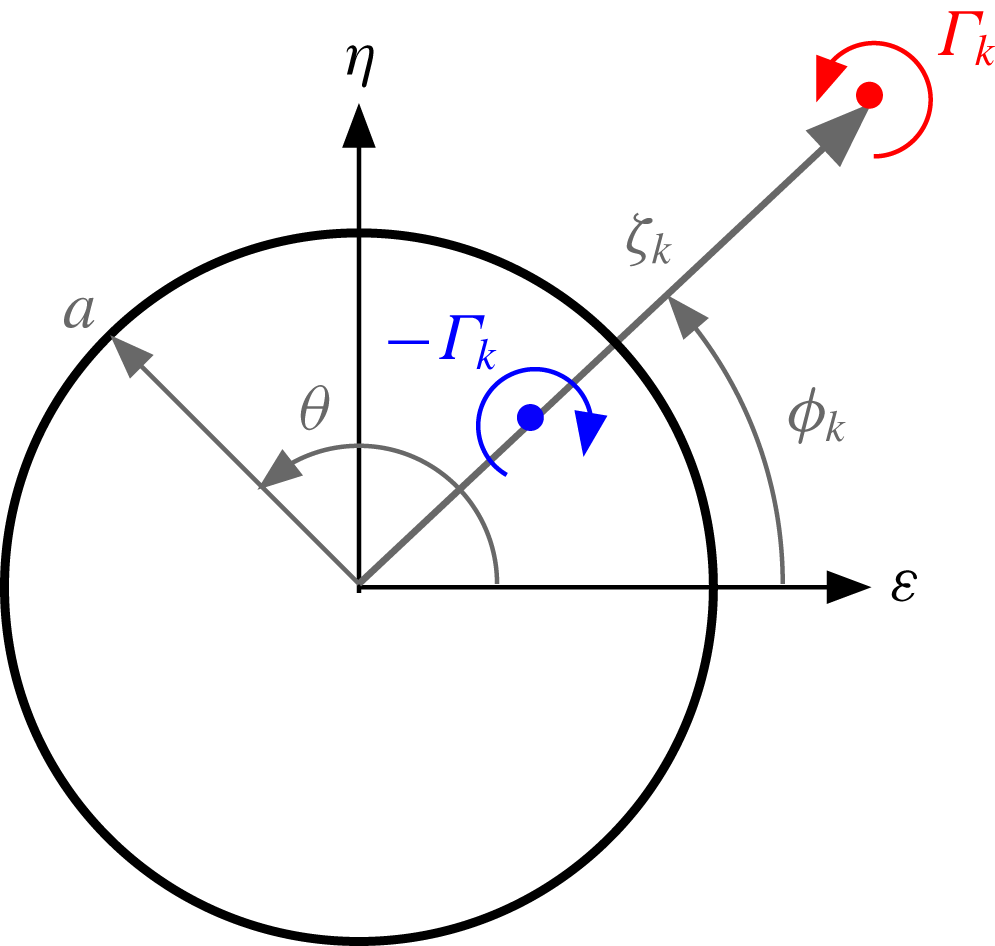
Schematic of a vortex element with circulation $\unicode[STIX]{x1D6E4}_{k}$ in the mapped circle frame, showing the corresponding ‘mirror’ with circulation $-\unicode[STIX]{x1D6E4}_{k}$ .

The circulatory vortex sheet constituent, $\unicode[STIX]{x1D6FE}^{c}$ , is found using the potential flow model described by Graham et al. (Reference Graham, Pitt Ford and Babinsky2017). External vortices are used to calculate the circulatory vortex sheet by their mirror images in a circle frame mapping of the flow field. This model is therefore ‘data-driven’, as the position and circulation of each external vortex will be determined using PIV data of a physical flow field. For complex geometries a panel code may be used to find the equivalent $\unicode[STIX]{x1D6FE}^{c}$ for a body subject to flow induced by external vortices; however, for a simple flat plate the mapping method allows an exact analytical expression to be derived. The plate is mapped to a circle with radius $a=c/4$ using the relation,

(2.5)

$$\begin{eqnarray}z=\unicode[STIX]{x1D701}+\frac{(c/4)^{2}}{\unicode[STIX]{x1D701}},\end{eqnarray}$$

where $\unicode[STIX]{x1D701}=\unicode[STIX]{x1D716}+\text{i}\unicode[STIX]{x1D702}$ , a position vector in the mapped frame. The mapped frame is illustrated in figure 5. In the mapped frame the circle is subject to the same condition as the plate (flow cannot pass through its surface and circulation is unchanged). As illustrated, a single vortex with circulation $\unicode[STIX]{x1D6E4}_{k}$ is located in the flow field at the position $\unicode[STIX]{x1D701}_{k}$ . This represents a single element from a field of vorticity. To satisfy the no-penetration condition, ‘mirror’ vortices must be placed inside the circle. This ensures that the circle circumference is a streamline of the flow by balancing the radial velocity component that the free vortex induces on the circle boundary. According to Saffman (Reference Saffman1992) there are an infinite number of mirror vortex combinations that satisfy this condition. The solution given by Graham et al. (Reference Graham, Pitt Ford and Babinsky2017) satisfies conservation of global circulation and the circle boundary condition with just a single mirror vortex of circulation $-\unicode[STIX]{x1D6E4}_{k}$ at a location $\unicode[STIX]{x1D701}_{k,mir}=(a^{2}/|\unicode[STIX]{x1D701}_{k}|)\text{e}^{\text{i}\unicode[STIX]{x1D719}_{k}}$ . The free vortex and its mirror may be used to find $\unicode[STIX]{x1D6FE}^{c}$ by calculating the surface slip velocities in the plate frame. These are obtained here using the complex potential method. The complex potential, defined as $F_{k}(\unicode[STIX]{x1D701})=\unicode[STIX]{x1D6F7}_{k}+\text{i}\unicode[STIX]{x1D6F9}_{k}$ with $\unicode[STIX]{x1D6F7}_{k}$ and $\unicode[STIX]{x1D6F9}_{k}$ being the potential function and streamfunction for the vortex pair, is

(2.6)

$$\begin{eqnarray}F_{k}(\unicode[STIX]{x1D701})=-\text{i}\frac{\unicode[STIX]{x1D6E4}_{k}}{2\unicode[STIX]{x03C0}}\ln \left(\frac{\unicode[STIX]{x1D701}-\unicode[STIX]{x1D701}_{k}}{\unicode[STIX]{x1D701}-\unicode[STIX]{x1D701}_{k,mir}}\right).\end{eqnarray}$$

The flow velocity ( $u_{k},v_{k}$ ) in the plate frame is given by

(2.7)

$$\begin{eqnarray}u_{k}-\text{i}v_{k}=\frac{\text{d}F_{k}}{\text{d}z}=\frac{\text{d}F_{k}}{\text{d}\unicode[STIX]{x1D701}}\left(\frac{\text{d}z}{\text{d}\unicode[STIX]{x1D701}}\right)^{-1}.\end{eqnarray}$$

Evaluating the derivatives yields

(2.8)

$$\begin{eqnarray}u_{k}-\text{i}v_{k}=\frac{\text{i}\unicode[STIX]{x1D6E4}_{k}}{2\unicode[STIX]{x03C0}}\frac{\unicode[STIX]{x1D701}^{2}(\unicode[STIX]{x1D701}_{k,mir}-\unicode[STIX]{x1D701}_{k})}{(\unicode[STIX]{x1D701}^{2}-(c/4)^{2})(\unicode[STIX]{x1D701}-\unicode[STIX]{x1D701}_{k,mir})(\unicode[STIX]{x1D701}-\unicode[STIX]{x1D701}_{k})}.\end{eqnarray}$$

To calculate the strength of the vortex sheet, the velocity tangential to the surface of the plate ( $u_{k}$ ) is required. The plate surface corresponds to the cylinder surface in the complex frame, given by $\unicode[STIX]{x1D701}=a\text{e}^{\text{i}\unicode[STIX]{x1D703}}$ . Therefore, at the plate surface equation (2.8) gives

(2.9)

$$\begin{eqnarray}u_{k}(\unicode[STIX]{x1D703})=\frac{-\unicode[STIX]{x1D6E4}_{k}}{\unicode[STIX]{x03C0}c\sin \unicode[STIX]{x1D703}}\frac{(c/4)^{2}-|\unicode[STIX]{x1D701}_{k}|^{2}}{|\unicode[STIX]{x1D701}_{k}|^{2}-{\textstyle \frac{1}{2}}|\unicode[STIX]{x1D701}_{k}|c\cos (\unicode[STIX]{x1D703}-\unicode[STIX]{x1D719}_{k})+(c/4)^{2}}.\end{eqnarray}$$

Here $\unicode[STIX]{x1D703}$ , the angle from the $\unicode[STIX]{x1D716}$ axis to a position on the cylinder surface (anticlockwise positive), is related to the plate frame by $x=(c/2)\cos \unicode[STIX]{x1D703}$ . The vortex sheet attributable to the vortex pair is equal to the velocity difference either side of the plate,

(2.10)

$$\begin{eqnarray}\unicode[STIX]{x1D6FE}_{k}^{c}(\unicode[STIX]{x1D703})=u_{k}(-\unicode[STIX]{x1D703})-u_{k}(\unicode[STIX]{x1D703}),\end{eqnarray}$$

with $0\leqslant \unicode[STIX]{x1D703}\leqslant \unicode[STIX]{x03C0}$ . Finally, an arbitrary number of vortices ( $n$ ) will be measured in the flow field, so the total circulatory vortex sheet is found by linear superposition,

(2.11)

$$\begin{eqnarray}\unicode[STIX]{x1D6FE}^{c}=\mathop{\sum }_{k=1}^{n}\unicode[STIX]{x1D6FE}_{k}^{c}.\end{eqnarray}$$

Because the location of each vortex is to come from PIV data in the plate frame, a conversion from the real to the mapped frame is needed. Solving for the roots of (2.5) gives the inverse mapping

(2.12)

$$\begin{eqnarray}\unicode[STIX]{x1D701}=\frac{z\pm \sqrt{z^{2}-4(c/4)^{2}}}{2}.\end{eqnarray}$$

As there are two solutions to (2.12), one inside the mapped circle and the other outside, only the outer solution ( $|\unicode[STIX]{x1D701}|\geqslant a$ ) is used.

2.3 Potential flow model summary

A potential model has been derived to obtain the distribution of boundary layer vorticity for a flat-plate wing undergoing arbitrary translation and rotation kinematic motions through a viscous and separated flow. The boundary layer is represented by a vortex sheet of strength $\unicode[STIX]{x1D6FE}^{b}=\unicode[STIX]{x1D6FE}^{nc}+\unicode[STIX]{x1D6FE}^{c}$ . Through linear superposition the non-circulatory term $\unicode[STIX]{x1D6FE}^{nc}$ consists of a component attributed to translation $\unicode[STIX]{x1D6FE}_{t}^{nc}$ , and another due to rotation $\unicode[STIX]{x1D6FE}_{r}^{nc}$ . The circulatory term $\unicode[STIX]{x1D6FE}^{c}$ is due to vorticity in the bulk flow field. Using PIV data it is possible to determine $\unicode[STIX]{x1D6FE}^{c}$ experimentally. It is apparent that, if the boundary layer vortex sheet $\unicode[STIX]{x1D6FE}^{b}$ can also be quantified experimentally, then the component directly attributable to added mass ( $\unicode[STIX]{x1D6FE}^{nc}$ ) may be isolated from flow field measurements. Further limiting the kinematic motion to just translation or rotation enables independent measurements of $\unicode[STIX]{x1D6FE}_{t}^{nc}$ and $\unicode[STIX]{x1D6FE}_{r}^{nc}$ to be obtained. These may then be compared to the theoretical distributions given by (2.4), thereby testing the validity of the potential flow solution for added mass in separated viscous flows.

Figure 6.

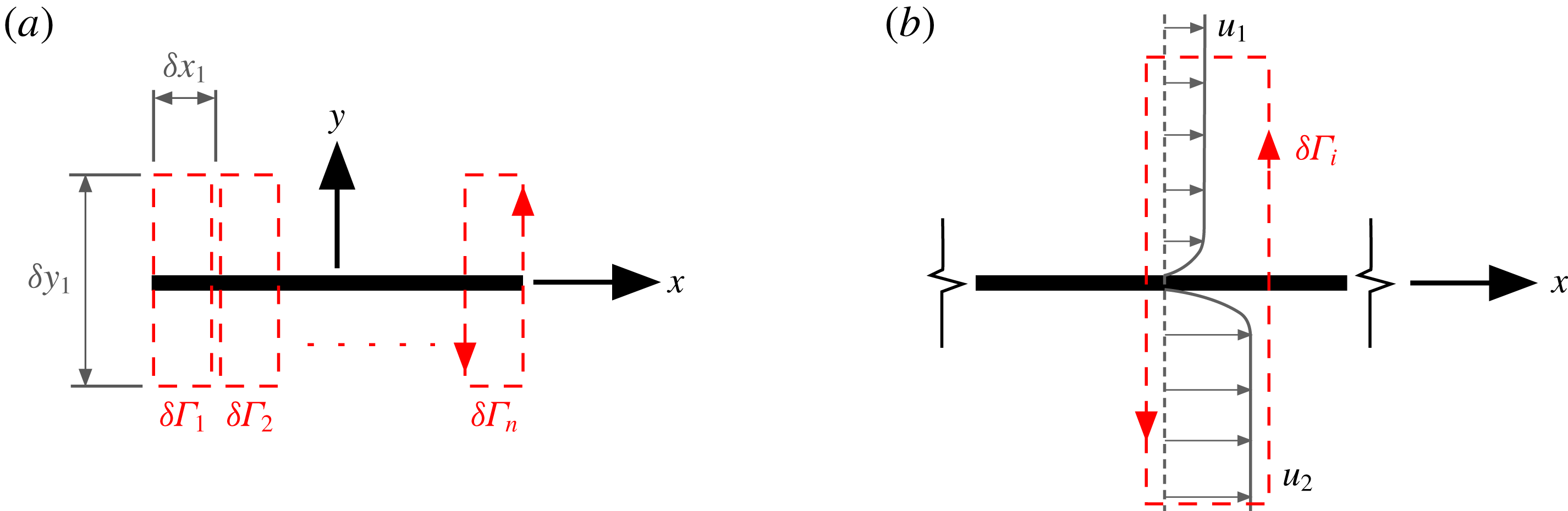
Elements used for the calculation of the boundary layer circulation: (a) overview showing integration contour elements distributed across the plate chord; (b) schematic showing a single integration element encompassing boundary layers.

3 Quantification of $\unicode[STIX]{x1D6FE}^{b}$ from particle image velocimetry

In the introductory section, it was observed that the difficulty with directly resolving the vorticity in the boundary layer using PIV (to obtain a measure of $\unicode[STIX]{x1D6FE}^{b}$ ) stems from the requirement that typically large regions of the flow field must be captured to include starting vortices. There is a compromise between field of view and spatial resolution, the former often taking priority. Furthermore, the added-mass attributed vorticity is generated in an ‘intensely concentrated’ region of the boundary layer adjacent to the wall. In this region the scattering of laser light from the surface results in a loss of measurements due to saturation of the camera sensor. With such an experimental set-up it is unlikely that velocity gradients within the boundary layer, and added-mass attributed vorticity in particular, can be resolved directly. It is, however, possible to infer the boundary layer vorticity by application of Stokes’ theorem,

(3.1)

$$\begin{eqnarray}\unicode[STIX]{x1D6E4}=\int _{A}\unicode[STIX]{x1D714}\,\text{d}A=\oint \boldsymbol{u}\boldsymbol{\cdot }\mathbf{d}\boldsymbol{l}.\end{eqnarray}$$

The surface integral of vorticity over an area $A$ (circulation) is equal to the closed line integral of the velocities about the circumference. Even for a near-singular and unmeasurable distribution of vorticity, the circulation can be determined by the entirely measurable flow field velocities nearby.

Figure 7.

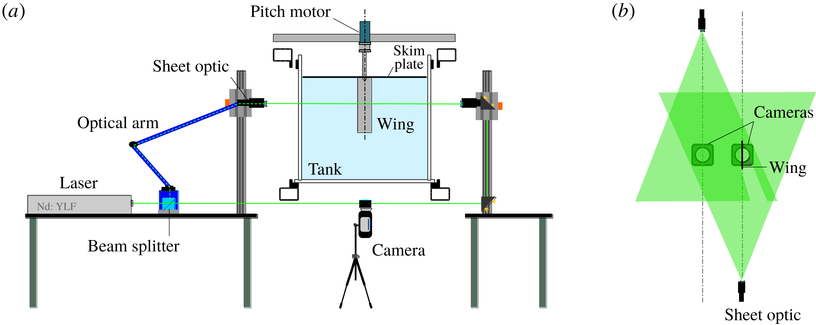
Schematic of towing tank, PIV and flow visualisation configurations: (a) end view; (b) top view showing the laser overlap plane and camera set-up. Adapted from Stevens & Babinsky (Reference Stevens and Babinsky2017).

With the present problem the ‘singularity’ is not a point vortex free in the flow field, but rather is in the form of a boundary layer over the surface of a plate. The question is what happens to the integration contour that crosses over the surface? In this case a body of finite cross-sectional area can be treated as an area of fluid with equivalent kinematic and geometric properties. When undergoing pure translation the ‘body fluid’ is irrotational and when in pure rotation it has uniform vorticity with magnitude twice the rate of angular rotation (Wu Reference Wu1981). Applying this condition allows an integration contour to cross over the body surface as if the flow field and body geometry were a continuum. The circulation of a segment of the boundary layer can therefore be measured. For the plate geometry, elements of circulation ( $\unicode[STIX]{x1D6FF}\unicode[STIX]{x1D6E4}_{n}$ ) are calculated using the contours of integration shown in figure 6(a). It is assumed here that the plate used for experiments is infinitely thin and no correction for finite thickness has been made. The circulation of vorticity contained in the boundary layer may then be equated to that of the vortex sheet, $\int _{A}\unicode[STIX]{x1D714}\,\text{d}A=\int \unicode[STIX]{x1D6FE}\,\text{d}x$ , and a local estimate of a boundary layer equivalent vortex sheet can be found by dividing the circulation of each element by the element width:

(3.2)

$$\begin{eqnarray}\unicode[STIX]{x1D6FE}_{n}^{b}\approx \unicode[STIX]{x1D6FF}\unicode[STIX]{x1D6E4}_{n}/\unicode[STIX]{x1D6FF}x_{n}.\end{eqnarray}$$

For the boundary layers shown in figure 6(b), application of this method returns a vortex sheet of strength $\unicode[STIX]{x1D6FE}_{n}^{b}=u_{2}-u_{1}$ . A measure of the integral boundary layer vorticity can therefore be obtained without requiring measurement of velocity gradients within the boundary layer. The spatial resolution (in the $x$ direction) is, however, limited by the underlying PIV grid resolution. For the current experiment, the plate was discretised into 50 area elements, over a distance of $1.0c$ in the $x$ direction ( $\unicode[STIX]{x1D6FF}x=0.02c$ ). This is similar to the PIV resolution, which is described later. Each element had a height of $\unicode[STIX]{x1D6FF}y=0.25c$ , which was selected as it is sufficiently large to include the boundary layer, while largely avoiding ‘free’ vorticity in the bulk flow field (shown later in figures 8 and 9). If any free vorticity is encompassed by the contours of integration, it will be excluded from the circulatory vortex sheet calculation $\unicode[STIX]{x1D6FE}^{c}$ , and is instead assigned as local boundary layer vorticity. This is to be avoided where possible.

4 Description of the experiments

PIV and flow visualisation experiments were performed on a flat plate undergoing linear acceleration at $90^{\circ }$ incidence (surge) and on a plate rotated ‘impulsively’ about the mid-chord. These experiments were selected to isolate the translation and rotation components of the non-circulatory vortex sheet, given by (2.4). Experiments were performed in the water towing tank shown schematically in figure 7(a). The plate has a chord of 120 mm, thickness of 4 mm and immersed span of 480 mm. While this gives a physical aspect ratio of 4, a skim plate was used on the upper end at the waterline to reduce free surface effects and give an effective aspect ratio of 8 due to the mirror effect. A stepping motor is used for pitch actuation.

For both test cases the added-mass force and flow field impulse acquired using PIV are compared with the theoretical potential flow equivalent. This requires knowledge of the kinematics of the plate in the measurement plane. For the surge case the instantaneous acceleration was measured using an ADXL335 three-component micro-electromechanical accelerometer embedded within the plate. Velocity was measured using a linear quadrature encoder with step resolution of 1 mm. Data from each of these sensors are acquired at 5 kHz. For the rotation experiment the angular position is assumed to be equal to the prescribed motion from the stepping motor. It should be noted that the plate is not infinitely stiff, so the prescribed and actual motions at the measurement plane can differ due to vibration. A more detailed analysis of vibration of the set-up is given by Corkery, Babinsky & Harvey (Reference Corkery, Babinsky and Harvey2018). The embedded accelerometer corrects for the vibration-attributed difference for the translation case; however, vibration and other discrepancies from the prescribed motion are unaccounted for in the rotation case.

4.1 PIV and flow visualisation

PIV was taken using a commercial LaVision Flowmaster two-dimensional PIV set-up. For the surge case a dual camera and a dual light sheet configuration as shown in figure 7(b) was used. This enabled the acquisition of vectors across the full plane without camera view obstruction or shadow region effects. A similar configuration was used for the rotating plate experiment; however, now the laser centre axes coincide and a single camera was used. Regions of the flow field obstructed from the field of view of a single camera were masked and the flow field in regions measured by both cameras was averaged. All PIV data were acquired at the physical mid-span of the wing and the flow is assumed to be two-dimensional. Titanium dioxide seeding particles were illuminated using a Nd:YLF 527 nm wavelength laser and recorded with a Phantom M310 camera. For the surge case the frame rate was 200 Hz, while 50 Hz was used for the rotation case. Vector fields for the surge case were computed using sequential image frames with an initial interrogation window of $64~\text{pixel}\times 64~\text{pixel}$ , followed by a nominal $16~\text{pixel}\times 16~\text{pixel}$ deformable interrogation window with two passes and 50 % overlap. For the rotation case the vector fields were computed using an initial window of $32~\text{pixel}\times 32~\text{pixel}$ , followed by two passes with a nominally $12~\text{pixel}\times 12~\text{pixel}$ deformable interrogation window and also 50 % overlap. Each PIV measurement presented is an ensemble average of five test runs. Dye flow visualisation was performed by injecting a milk-based dye mixture at points where flow is entrained into the shear layer leaving the edges of the plate. For the surge case, the injection locations were approximately 4 mm from each plate edge, on the leeward face. For the rotation case dye was injected on the advancing faces at an equivalent location. Dye was illuminated with the dual laser light sheet described above, albeit with a defocused beam width of approximately 20 mm to allow for illumination of dye that has advected slightly in the spanwise direction.

4.2 Plate kinematics

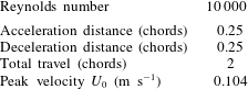
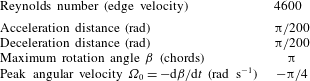
General kinematic parameters for the surge and rotation cases are given in tables 1 and 2, respectively. For the surging profile the plate underwent nominally constant acceleration over a distance of 0.25 chord lengths, travelled at constant velocity for 1.5 chord lengths and decelerated over a distance of 0.25 chords. The total travel distance is thus 2 chords. Both the dye flow visualisation and PIV were carried out at a Reynolds number of 10 000 as calculated from the peak velocity. For the rotation case, the plate was nominally ‘impulsively’ rotated in the clockwise direction from rest to a constant angular velocity ( $\unicode[STIX]{x1D6FA}=-\unicode[STIX]{x03C0}/4~\text{rad}~\text{s}^{-1}$ ) about an axis at the mid-chord. Based on the plate chord and edge velocity the Reynolds number is 4600. After rotating $180^{\circ }$ the plate was impulsively decelerated to rest. It is recognised that a perfectly impulsive motion is impossible due to both finite plate stiffness and torque limitations. For the calculations of pitching moment using potential theory, it is assumed that the angular acceleration is constant over a time equal to the PIV sample period (0.02 s). Based on the stepping motor commanded motion, the actual acceleration period is likely to be lower than 0.02 s, but PIV-based measures of impulse are limited by the camera frame rate, so the same limitation is placed on the potential theory-based estimate.

Table 1.

Surging plate kinematics.

Table 2.

Rotating plate kinematics.

5 Results

5.1 Flow topology

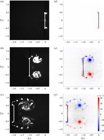
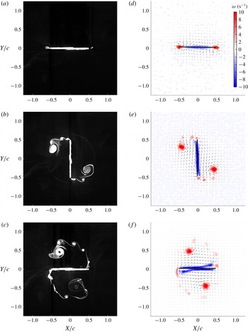
Dye flow visualisation and PIV for the surging case are shown in figure 8, while figure 9 gives the corresponding measurements for the rotation case. The PIV data show contours of vorticity (red, anticlockwise positive; blue, negative) and arrows with flow direction. For each data element, the vorticity was calculated by taking the trapezoidal closed line integral of velocity through the centroid of each adjacent element (size $2\unicode[STIX]{x0394}l\times 2\unicode[STIX]{x0394}l$ , where $\unicode[STIX]{x0394}l$ is the data point element width). This gives a circulation, which divided by the area enclosed by the integration contour ( $4\unicode[STIX]{x0394}l^{2}$ ) gives the vorticity.

In the surge case the following can be observed.

(i) At $X_{c}/c=-0.02$ , the plate undergoes maximum acceleration but still has low velocity. The start of two vortices is visible in the flow field. PIV shows a (faint) region of negative vorticity at the top half of the plate and positive vorticity on the lower half.
(ii) At $X_{c}/c=-1.00$ , the plate is translating at constant velocity. A pair of counter-rotating vortices behind the upper and lower plate edges are visible in both the dye flow and PIV. Clear regions of boundary layer vorticity are visible in the PIV, but cannot be seen in the flow visualisation.
(iii) At $X_{c}/c=-1.98$ , the plate has decelerated to almost a complete stop. The pair of vortices has moved downstream relative to the plate and the shear layers feeding each vortex can be seen. Discrete blobs of dye are visible in the shear layer; these are the result of the Kelvin–Helmholtz instability and show the accumulation of vorticity from the shear layer into discrete rollers. Again, there is a clear region of boundary layer vorticity. This appears to be shedding off the plate edges as the plate is near rest and flow induced by the primary vortices moves in the $-X$ direction.

For the rotation case the following can be observed.

(i) At $\unicode[STIX]{x1D6FD}\approx 1^{\circ }$ , the plate has started motion and is rotating at constant angular velocity. The dye flow visualisation does not show any vortices in the flow field. The PIV, however, shows a strong distribution of positive vorticity at the plate edges and negative vorticity towards the centre.
(ii) At $\unicode[STIX]{x1D6FD}=90^{\circ }$ , the plate is midway through the rotation and is moving at constant angular velocity. A positive vortex, fed by a visible shear layer, has shed at each plate edge. Again a Kelvin–Helmholtz instability is seen. There are clearly defined regions of negative boundary layer vorticity visible in the PIV, which are not seen in the dye flow visualisation.
(iii) At $\unicode[STIX]{x1D6FD}=180^{\circ }$ , the plate is travelling at constant angular velocity, but is about to encounter the deceleration impulse. The pair of vortices has moved further ‘downstream’ relative to the circumferential path of the plate edges. The Kelvin–Helmholtz instability is less coherent. This appears to be a result of secondary flow separation interacting with the primary shear layer. The secondary separation can be seen by the thickening of the negative boundary layer vorticity towards the plate edges.

Both the surge and rotation test cases have shown distributions of boundary layer vorticity during their motions. It is this vorticity that is expected to have a component attributable to the added-mass effect. In the following sections this component is quantified and compared with potential theory.

Figure 8.

Dye flow visualisation (a–c) and PIV flow field measurements (d–f) for the surge test case: (a,d) $X_{c}/c=-0.02$ ; (b,e) $X_{c}/c=-1.00$ ; (c,f) $X_{c}/c=-1.98$ . Only every fourth velocity vector is shown; $Re=10\,000$ .

Figure 9.

Dye flow visualisation (a–c) and PIV flow field measurements (d–f) for the rotating plate case: (a,d) $\unicode[STIX]{x1D6FD}\approx 1^{\circ }$ ; (b,e) $\unicode[STIX]{x1D6FD}=90^{\circ }$ ; (c,f) $\unicode[STIX]{x1D6FD}=180^{\circ }$ . Only every fourth velocity vector is shown. $Re=4600$ .

5.2 Single-sided flow field circulation

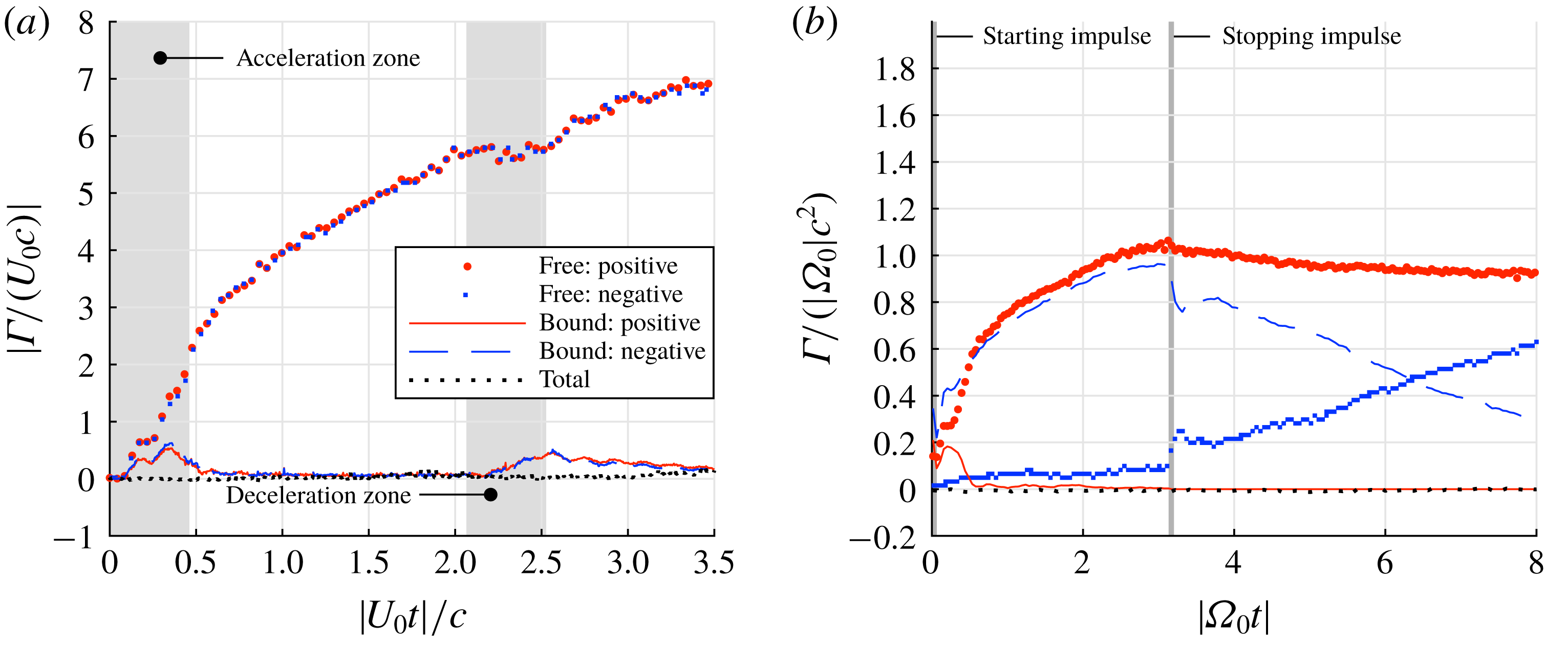
Separate sums of positive and negative elements of circulation in the flow field are plotted in figure 10. The circulation elements are categorised as those that are ‘bound’, which means they are included in the boundary layer areas of integration described in § 3, and those that are ‘free’, i.e. in the bulk flow field. Both test cases show zero total circulation throughout the measurement period, as expected. In figure 10(b) the discontinuities in circulation components at the start and end of the angular motion suggest that added-mass attributable vorticity is captured by the PIV data bracketing each acceleration period. After the deceleration impulse at $|\unicode[STIX]{x1D6FA}_{0}t|=\unicode[STIX]{x03C0}$ the gradual increase in negative free circulation, and reduction in bound negative circulation, result from the formation of a stopping vortex shed at each edge of the plate.

Figure 10.

Sums of the boundary layer and bulk flow circulation elements: (a) surge case; (b) rotation case.

5.3 Non-circulatory vortex sheets

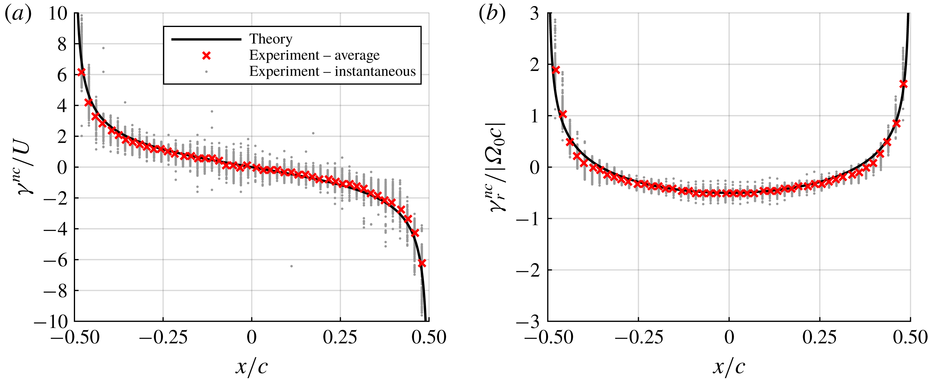
The added-mass vortex sheet $\unicode[STIX]{x1D6FE}^{nc}$ is obtained by taking direct measurements of the boundary layer vortex sheet $\unicode[STIX]{x1D6FE}^{b}$ and subtracting the component attributed to free vorticity in the flow field $\unicode[STIX]{x1D6FE}^{c}$ (refer to §§ 2 and 3). In potential flow theory the theoretical added-mass vortex sheet is proportional to the respective translation or angular velocities (see (2.4)). Acceleration of the plate creates the vortex sheet, but once constant velocity is reached it will persist unchanged. Therefore, by normalising the added-mass vortex sheet strength with the kinematic velocity, it is possible to obtain a universal distribution that is independent of both velocity and acceleration rate. This is the ‘theory’ line given in figure 11. If, as expected, the experimental measurements of the added-mass vorticity are also independent of viscous effects such as separation, the normalised measurements should also be constant. This is advantageous as a sequential average may be taken to reduce random error attributable to measurement noise. For the surge case the average of frames between $X_{c}/c=-0.02$ and $X_{c}/c=-1.98$ is taken (530 measurements). The very start ( $-0.02\leqslant X_{c}/c\leqslant 0$ ) and end of motion ( $-2\leqslant X_{c}/c\leqslant -1.98$ ) are avoided to prevent normalising the measured added-mass vortex sheet by vanishingly small velocity values. For the rotating case, frames between $\unicode[STIX]{x1D6FD}=1^{\circ }$ and $\unicode[STIX]{x1D6FD}=179^{\circ }$ are used (approximately 100 measurements). The normalised, experimentally attained, added-mass vortex sheets are included in figure 11. This is in striking agreement with the theoretical distribution.

Figure 11.

Comparison of measured and potential flow vortex sheets between potential theory and experiment for the surge (a) and rotation (b) cases.

The agreement between measurement and theory shows that vorticity is generated in the physical flow field when the plate is accelerated, with a distribution close (if not identical) to that predicted with inviscid theory. It can further be deduced that the distribution of this non-circulatory vortex sheet is unchanged by viscous effects and the corresponding changes to flow topology because most of the measurements utilised in the averaging process were taken when the flow was in a state of severe separation. This can be shown more clearly by considering the instantaneous PIV.

5.4 Instantaneous non-circulatory vortex sheet

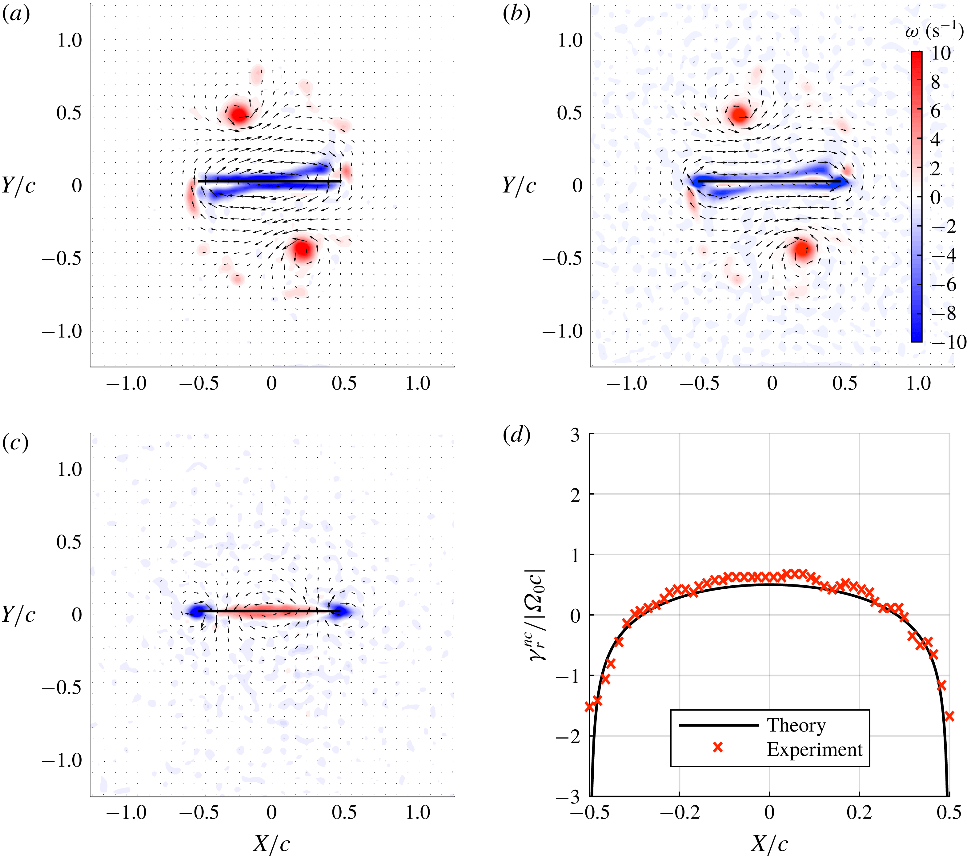
To demonstrate further that the inviscid added-mass vortex sheet distribution is also correct for a fully developed viscous flow field with significant separation, and hence with considerable topological differences from the potential flow, the flow field over the deceleration impulse for the rotation case is considered. Figure 12(a) shows the flow field before the deceleration impulse ( $\unicode[STIX]{x1D6FD}=180^{\circ -}$ ) and figure 12(b) shows the flow field immediately after ( $\unicode[STIX]{x1D6FD}=180^{\circ +}$ ). The flow fields are similar, with the strengths and positions of each shed vortex practically unchanged; however, there is a slight difference in the vorticity near the surface of the plate.

Obviously some change must have happened to the flow field when the plate is suddenly brought to rest in order to satisfy the no-penetration condition. This change can be identified by taking the difference in the flow field before and after the impulse. The change to the flow field is shown in figure 12(c) and the corresponding change to the boundary layer vortex sheet is given by figure 12(d). It is immediately visible that the change made to the flow field is equivalent, albeit inverse, to that produced during the starting motion shown previously in figure 9(d). Over the deceleration period the topological change to the flow field has resulted in the creation of non-circulatory boundary layer vorticity, which exactly destroys that created during the initial acceleration phase (see figures 9 d and 11 b). It can therefore be concluded that, even in a highly separated viscous flow field, changes due to acceleration are equivalent to those of potential flow. The evidence thus confirms that the added-mass force on the plate (or flow field) is equivalent to the potential solution for all flows, whether inviscid and attached, or viscous with significant separation.

The rotation case has also revealed a second method for quantifying the added-mass vorticity. Taking the difference between consecutive PIV frames isolates changes in vorticity including those attributable to diffusion, advection, experimental noise and added-mass effects. For bodies undergoing high rates of acceleration the latter source is dominant. The distribution of added-mass attributed vorticity, generated due to a change in velocity between consecutive measurement frames, may then be quantified directly using the methodology described in § 3. This approach is less rigorous than the potential flow-based model described in § 2, but is significantly simpler to implement and may be useful in situations where there are large accelerations.

Figure 12.

PIV data of the flow field at $\unicode[STIX]{x1D6FD}=180^{\circ }$ : (a) before the deceleration impulse, $\unicode[STIX]{x1D6FD}=180^{\circ -}$ ; (b) after the impulse, $\unicode[STIX]{x1D6FD}=180^{\circ +}$ ; (c) the change to the flow field for the rotation test case; (d) the change to the bound vortex sheet across the deceleration impulse compared with potential theory. Only every fourth PIV vector is shown.

5.5 Impulse and forces from PIV

Since it is possible to extract the added-mass attributable vortex sheets for each PIV frame, the added-mass contribution to the flow field impulse and forces can be quantified and compared with potential theory. Discretisation of the measured vortex sheet, however, can result in significant errors. As shown in figure 11, the measured vortex sheet is truncated at the edges, whereas the theoretical distribution tends to infinity. As a result, an integration of the measured vortex sheet using the discrete points can give errors up to 25 %. To compensate, an analytical function is fitted to the experimental data, which reduces the error to approximately 5 %. Further details, and the quantification of errors using an artificial flow field, are given in § B.1. The impulse for the ‘full’ flow field, that is, the sum of the contributions of bound and free vorticity, is found directly from the elemental vorticity, as discretisation errors are comparatively negligible. Theoretical impulse and force values are calculated using the potential flow solution derived in appendix A. For the surge case, the kinematics are based on sensor data. For the rotation case the kinematics are equal to the prescribed plate motion, as a measure of actual kinematics is unavailable.

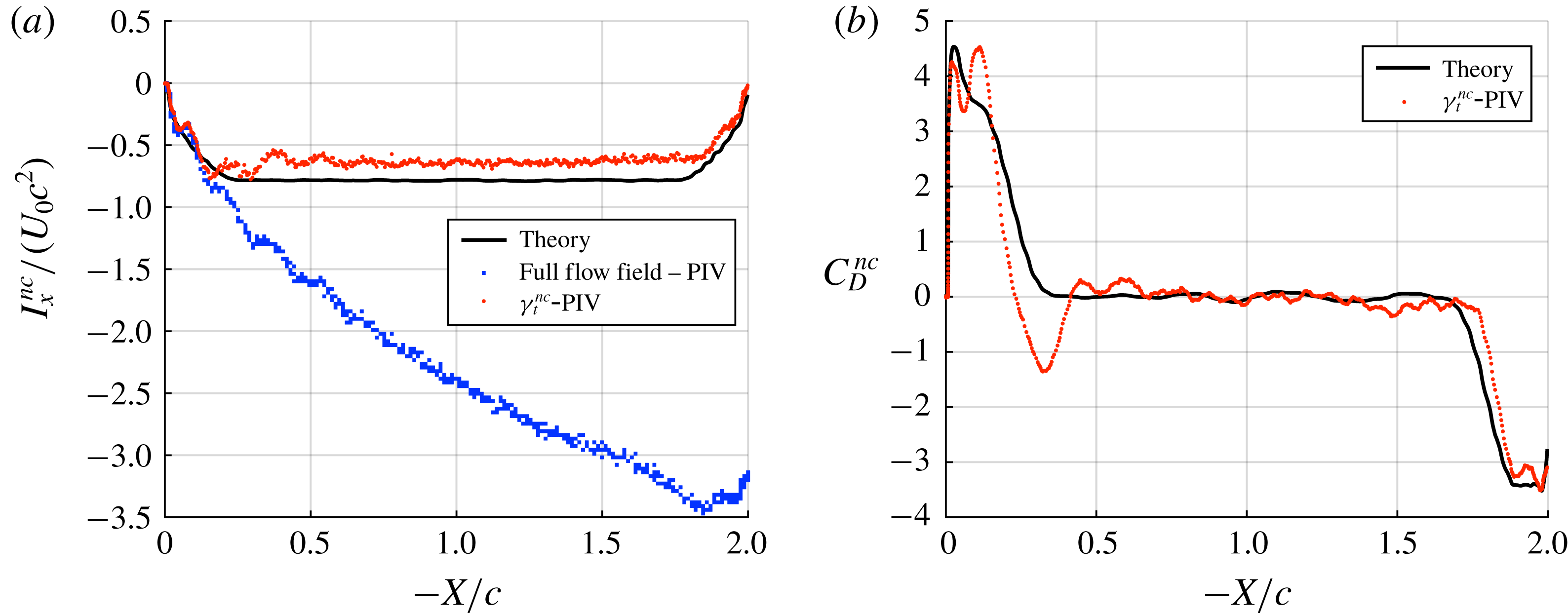
The impulse for the surge case is shown in figure 13(a). During the initial acceleration period $0\leqslant -X_{c}/c\leqslant 0.25$ , the impulse from all three methods matches relatively well. This implies that added-mass effects are dominant. The impulse based on PIV shows some oscillations, which are the result of wing vibration. During the constant-velocity phase $0.25\leqslant -X_{c}/c\leqslant 1.75$ the measure of the impulse from the PIV-derived non-circulatory vortex sheet ( $\unicode[STIX]{x1D6FE}_{t}^{nc}$ -PIV) fits theory relatively well, albeit being slightly lower in magnitude. Given the excellent fit initially, this may be the result of slight three-dimensional effects. Over the deceleration region, agreement between $\unicode[STIX]{x1D6FE}_{t}^{nc}$ -PIV and theory is reasonable. The drag force coefficient attributed to added mass is given in figure 13(b). There is relatively good agreement across the range of the experiment, albeit the PIV-derived measurement is significantly lower than theory in the range $0.25\leqslant -X_{c}/c\leqslant 0.5$ .

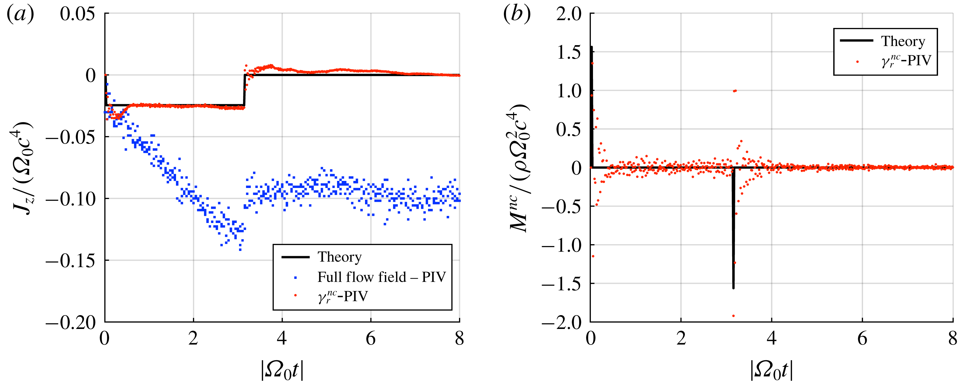
For the rotation case the first moment of impulse is given by figure 14(a). Considering the full flow field, the regions of high angular acceleration at the start ( $|\unicode[STIX]{x1D6FA}_{0}t|=0$ ) and end of plate kinematic motion ( $|\unicode[STIX]{x1D6FA}_{0}t|=\unicode[STIX]{x03C0}$ ) are clearly evident as discontinuities in the first moment of impulse. During the phase of constant angular rotation, the evolution of the first moment of impulse is remarkably linear. Now considering the added-mass-only components, there is excellent agreement between the theoretical first moment of impulse and that derived from the measure of the non-circulatory vortex sheet ( $\unicode[STIX]{x1D6FE}_{r}^{nc}$ -PIV). The magnitude of the discontinuities at the start and end of kinematic motion are relatively accurately captured by the measured vortex sheet. Furthermore, $\unicode[STIX]{x1D6FE}_{r}^{nc}$ -PIV deviates little from theory over the constant angular velocity region. Further agreement between theory and experiment for the added-mass attributable pitching moment is shown in figure 14(b). As predicted, the measured moment ( $\unicode[STIX]{x1D6FE}_{r}^{nc}$ -PIV) is approximately zero for the entirety of the motion, except during the acceleration impulses. The scattering of $\unicode[STIX]{x1D6FE}_{r}^{nc}$ -PIV after each acceleration impulse decays asymptotically, which suggests that it is caused by damped torsional vibration of the plate.

Figure 13.

Surge case: (a) impulse compared between potential theory, the experimentally measured full flow field and the measured non-circulatory bound vortex sheet; (b) comparison of the added-mass attributed drag force coefficient between theory and the measured non-circulatory bound vortex sheet. For clarity, drag force coefficients are filtered using a bidirectional moving window average with a window period of 0.15 s.

Figure 14.

Rotation case: (a) first moment of impulse compared between potential theory, the experimentally measured full flow field and the measured non-circulatory bound vortex sheet; (b) comparison of the added-mass attributed pitching moment between theory and the measured non-circulatory bound vortex sheet. No filtering is employed.

6 Lost circulation compensation

In this work, excellent agreement has been demonstrated between measures of the non-circulatory vortex sheet, impulse and force with potential theory. This would not have been the case if the circulation measured within the flow field were not conserved (see § 5.2). The circulatory vortex sheet $\unicode[STIX]{x1D6FE}^{c}$ has a net circulation equal and opposite to that of all the bulk flow vorticity. The methodology for determining $\unicode[STIX]{x1D6FE}^{c}$ described in § 2.2.2 is based on the premise that the position and circulation of each bulk flow vortex element can be measured. Errors arise when a vortex element leaves the measurable field of view, which causes the circulation of $\unicode[STIX]{x1D6FE}^{c}$ to change in error by the circulation ‘lost’. Fortunately it is possible to partially compensate for this effect. Consider a flow field comprising of just the plate and a free vortex of circulation $\unicode[STIX]{x1D6E4}_{k}$ , both within an area $A$ that represents the measurable field of view. The plate must have a circulation of $-\unicode[STIX]{x1D6E4}_{k}$ . If the total circulation within $A$ ( $\unicode[STIX]{x1D6E4}_{in}$ ) is found using a closed contour of integration,

(6.1)

$$\begin{eqnarray}\unicode[STIX]{x1D6E4}_{in}=\oint _{A}\boldsymbol{u}\boldsymbol{\cdot }\mathbf{d}\boldsymbol{l},\end{eqnarray}$$

then $\unicode[STIX]{x1D6E4}_{in}$ will be zero. Now if the free vortex moves outside of $A$ , calculation of $\unicode[STIX]{x1D6E4}_{in}$ will return a non-zero result (the circulation of the plate). The net circulation outside of the observable area $A$ ( $\unicode[STIX]{x1D6E4}_{out}$ ), must be equal and opposite to that measured within $A$ to conserve circulation across the whole flow field:

(6.2)

$$\begin{eqnarray}\displaystyle \unicode[STIX]{x1D6E4}_{out} & = & \displaystyle -\unicode[STIX]{x1D6E4}_{in}\end{eqnarray}$$

(6.3)

$$\begin{eqnarray}\displaystyle & = & \displaystyle -\oint _{A}\boldsymbol{u}\boldsymbol{\cdot }\mathbf{d}\boldsymbol{l}.\end{eqnarray}$$

The circulation lost outside the measurement window is therefore determinable; however, its position is unknown. The lost circulation could be in the form of a single point vortex outside the observation window, or arbitrarily distributed. As described in § 2.2.2, the location of each external vortex and the mirror vortices within the mapped circle must be known to calculate the distribution of $\unicode[STIX]{x1D6FE}^{c}$ . However, it could be assumed that the vorticity outside the measurement window is sufficiently far from the plate that it is effectively at infinity. A single mirror vortex of circulation $-\unicode[STIX]{x1D6E4}_{out}$ would therefore be placed at the circle origin. This may not be unreasonable if there is a relatively large measurement field of view either side of the plate. The vortex sheet $\unicode[STIX]{x1D6FE}_{m}^{c}$ that arises due to the missing circulation can be found from (2.10) with the condition that the position of the external vortex $\unicode[STIX]{x1D701}_{k}\rightarrow \infty$ and replacing $\unicode[STIX]{x1D6E4}_{k}$ with $\unicode[STIX]{x1D6E4}_{out}$ . Equation (2.10) becomes

(6.4)

$$\begin{eqnarray}\unicode[STIX]{x1D6FE}_{m}^{c}=\frac{-\unicode[STIX]{x1D6E4}_{out}}{\unicode[STIX]{x03C0}\sqrt{\left({\displaystyle \frac{c}{2}}\right)^{2}-x^{2}}}.\end{eqnarray}$$

The contribution to the circulatory vortex sheet of vortices that have drifted outside the measurement window can therefore be approximated. More sophisticated corrections might also be possible in specific cases, if the location of the lost vorticity is approximately known.

7 Conclusion

Added mass is an unsteady fluid dynamic effect that has been discussed in the literature for over a century. Despite being initially characterised for an inviscid fluid, it is equally applicable for viscous and highly separated flows, a point that has been theoretically argued, but never experimentally demonstrated. In this paper we propose a method for isolating vorticity attributed to added mass using PIV. The technique does not require impractically high-resolution PIV data, as velocity gradients within the boundary layer need not be resolved. The method was applied to separate surging and rotating flat-plate wing kinematic cases. Excellent agreement between the PIV-acquired and potential theory-derived added-mass attributed vorticity was shown. Fair agreement was also found between the theoretical and measured impulse and force. The measurements therefore demonstrate the applicability of the potential flow result for viscous and highly separated flows. It may be concluded that viscous effects (diffusion and consequently the advection of vorticity from the surface of a body) result in the transport of vorticity into the wake. Viscous effects are therefore accounted for by the ‘circulatory’ terms: the measure of free vorticity and the calculated circulatory attached vortex sheet. The added-mass vortex sheets are dependent only on the body geometry and kinematics, and may be recovered experimentally after accounting for the circulatory terms.

While this work in part simply experimentally confirms existing theories, it also represents a significant advance in our understanding of the capabilities of PIV to quantify unsteady external flows. In particular, it shows that with careful experimental design the added-mass effect may be intentionally captured; or, equivalently, that vorticity or circulation attributable to the added-mass phenomenon may be a source of ‘contamination’ when determining the circulation of vortices shed into a flow field. For the calculation of the circulation of a vortex close to the surface of a body using closed contours of integration, contours that cross or are interpolated over the boundaries of a body will include added-mass effects regardless of body-containing vector treatment.

With the availability of complete PIV velocity field information of unsteady aerodynamic experiments, such as that described in this paper, it is suggested that velocity vectors within a body in the flow field be prescribed a velocity equal to the rigid-body kinematics instead of simple masking. Vorticity subsequently calculated will include a distribution attributable to the added-mass mechanism, albeit spatially averaged over each wall element. Measures of integral quantities such as impulse and force derived from the flow field vorticity will incorporate added-mass effects. Such measures have surprisingly little error for reasonable PIV vector resolutions.

Complete velocity field information may, however, not be available. Many PIV datasets have incomplete or spurious velocities near a body due to shadow effects and surface reflections. Since added mass is an effect that is quantified by boundary vorticity, the masking of vectors close to a body will remove its contribution to the impulse and forces subsequently derived. For incomplete vector fields, this work therefore supports the correction method developed by Graham et al. (Reference Graham, Pitt Ford and Babinsky2017), which utilises the potential flow vortex sheet to augment a separated viscous flow field.

Acknowledgements

The authors would like to acknowledge Schlumberger Limited, Churchill College and the Cambridge Commonwealth Trusts for funding this work.

Appendix A.

The potential flow about an ellipse undergoing arbitrary translation and rotation about the centroid is given in various forms by Lamb (Reference Lamb1895) and Milne-Thomson (Reference Milne-Thomson1986). In this appendix we start from the complex potential given by Milne-Thomson (Reference Milne-Thomson1986), and take the limiting case where the ellipse thickness is zero to obtain flow velocities, bound vortex sheet distributions as well as net flow field impulse and force for a flat plate.

A.1 General solution

In a manner similar to the derivation for flow about a plate due to an external point vortex derived in § 2.2.2, conformal mapping will be used to find the flow field about the plate. Positions in the circle plane are once again $\unicode[STIX]{x1D701}=\unicode[STIX]{x1D716}+\text{i}\unicode[STIX]{x1D702}$ , while positions in the plate plane are $z=x+\text{i}y$ . The transform

(A 1)

$$\begin{eqnarray}z=\frac{c}{4}\left(\unicode[STIX]{x1D701}+\frac{1}{\unicode[STIX]{x1D701}}\right),\end{eqnarray}$$

maps a circle with unit radius to a flat plate with chord $c$ . The complex potential, $F(\unicode[STIX]{x1D701})=\unicode[STIX]{x1D719}+\text{i}\unicode[STIX]{x1D713}$ , is

(A 2)

$$\begin{eqnarray}F(\unicode[STIX]{x1D701})=-A\unicode[STIX]{x1D701}^{-1}-B\unicode[STIX]{x1D701}^{-2},\end{eqnarray}$$

with

(A 3a,b )

$$\begin{eqnarray}A=\text{i}U_{n}\frac{c}{2},\quad B=\frac{\unicode[STIX]{x1D6FA}}{4}\left(\frac{c}{2}\right)^{2}.\end{eqnarray}$$

The complex velocity about the plate, $u-\text{i}v$ , is given by $\text{d}F/\text{d}z$ . Using the chain rule and equations (A 1) and (A 2) gives

(A 4)

$$\begin{eqnarray}u-\text{i}v=\frac{A\unicode[STIX]{x1D701}+2B}{{\displaystyle \frac{c}{4}}\unicode[STIX]{x1D701}(\unicode[STIX]{x1D701}^{2}-1)}.\end{eqnarray}$$

A.2 Surface velocity and bound vortex sheet

The surface of the plate corresponds to the circumference of the circle in the circle plane, defined by

(A 5)

$$\begin{eqnarray}\unicode[STIX]{x1D701}=\text{e}^{\text{i}\unicode[STIX]{x1D703}}.\end{eqnarray}$$

Substituting (A 5) and (A 3) into (A 4) gives the velocity on the surface of the plate as a function of the angle $\unicode[STIX]{x1D703}$ , angular velocity $\unicode[STIX]{x1D6FA}$ and the plate-normal velocity $U_{n}$ . Separating into real and imaginary terms and simplifying yields

(A 6)

$$\begin{eqnarray}\frac{\text{d}F}{\text{d}z}=\overbrace{U_{n}{\displaystyle \frac{\cos \unicode[STIX]{x1D703}}{\sin \unicode[STIX]{x1D703}}}+\unicode[STIX]{x1D6FA}{\displaystyle \frac{c}{4}}\frac{\cos 2\unicode[STIX]{x1D703}}{\sin \unicode[STIX]{x1D703}}}^{u}-\text{i}\overbrace{\left(U_{n}+\unicode[STIX]{x1D6FA}{\displaystyle \frac{c}{2}}\cos \unicode[STIX]{x1D703}\right)}^{v}.\end{eqnarray}$$

Because the plate is oriented on the $x$ axis, the vertical component $v$ is equal to the plate velocity while the horizontal component $u$ is equal to the instantaneous surface ‘slip’ velocity. The vortex sheet, defined in § 2.2, is equal to the difference in the horizontal velocity component either side of the plate:

(A 7)

$$\begin{eqnarray}\unicode[STIX]{x1D6FE}^{nc}(\unicode[STIX]{x1D703})=\underbrace{-2U_{n}\frac{\cos \unicode[STIX]{x1D703}}{\sin \unicode[STIX]{x1D703}}}_{translation}-\underbrace{\unicode[STIX]{x1D6FA}\frac{c}{2}\frac{\cos 2\unicode[STIX]{x1D703}}{\sin \unicode[STIX]{x1D703}}}_{rotation}.\end{eqnarray}$$

This expression is valid for the range $0\leqslant \unicode[STIX]{x1D703}\leqslant \unicode[STIX]{x03C0}$ . The $\sin \unicode[STIX]{x1D703}$ terms in the denominators of both the translation and rotation components indicate that the magnitude of the vortex sheet is infinite at the plate edges.

To relate the polar coordinates back to Cartesian we use the mapping relation given by (A 1). Substituting $\unicode[STIX]{x1D701}=\text{e}^{\text{i}\unicode[STIX]{x1D703}}$ gives

(A 8)

$$\begin{eqnarray}z=x=\frac{c}{2}\cos \unicode[STIX]{x1D703}.\end{eqnarray}$$

The vortex sheet strength may be written in terms of the Cartesian coordinate $x$ ,

(A 9)

$$\begin{eqnarray}\unicode[STIX]{x1D6FE}^{nc}(x)=\underbrace{-2U_{n}\frac{x}{\sqrt{(c/2)^{2}-x^{2}}}}_{translation}-\underbrace{\unicode[STIX]{x1D6FA}\frac{2x^{2}-(c/2)^{2}}{\sqrt{(c/2)^{2}-x^{2}}}}_{rotation}.\end{eqnarray}$$

A.3 Linear impulse and force

From the bound vortex sheet the flow field impulse (or ‘first moment of vorticity’) and force may be found using the relations given by Wu (Reference Wu1981). For a continuous two-dimensional vorticity distribution the relations are

(A 10a,b )

$$\begin{eqnarray}I_{x}=\int _{A}y\unicode[STIX]{x1D714}\,\text{d}A,\quad I_{y}=-\int _{A}x\unicode[STIX]{x1D714}\,\text{d}A.\end{eqnarray}$$

For a vortex sheet the impulse components become line integrals,

(A 11a,b )

$$\begin{eqnarray}I_{x}=\int y\unicode[STIX]{x1D6FE}(x,y)\,\text{d}l,\quad I_{y}=-\int x\unicode[STIX]{x1D6FE}(x,y)\,\text{d}l,\end{eqnarray}$$

where $l$ represents the distance along the sheet. Here, the sheet is restricted to the $x$ axis, $\text{d}l=\text{d}x$ and $I_{x}=0$ . The integral for $I_{y}$ can be evaluated by expressing the integral in polar form. The result is

(A 12)

$$\begin{eqnarray}I_{y}=\unicode[STIX]{x03C0}\frac{c^{2}}{4}U_{n}.\end{eqnarray}$$

From (A 12) it can be seen that the flow field impulse is independent of the angular velocity of the plate and is proportional to its normal velocity $U_{n}$ . The force on the plate is

(A 13)

$$\begin{eqnarray}\displaystyle F_{y} & = & \displaystyle -\unicode[STIX]{x1D70C}\frac{\text{d}I_{y}}{\text{d}t}\nonumber\\ \displaystyle & = & \displaystyle -\unicode[STIX]{x1D70C}\unicode[STIX]{x03C0}\frac{c^{2}}{4}\frac{\text{d}U_{n}}{\text{d}t}.\end{eqnarray}$$

A.4 First moment of impulse and mid-chord moment

In a similar manner the pitching moment about the mid-chord of the plate can be found. From Wu (Reference Wu1981), the second moment of vorticity, $\unicode[STIX]{x1D6FD}$ , for a continuous vorticity field in two dimensions is

(A 14)

$$\begin{eqnarray}\unicode[STIX]{x1D6FD}_{z}=\int _{A}(x^{2}+y^{2})\unicode[STIX]{x1D714}\,\text{d}A.\end{eqnarray}$$

Writing this as a line integral and substituting the polar forms of the integrand components, we obtain

(A 15)

$$\begin{eqnarray}\unicode[STIX]{x1D6FD}_{z}=-\frac{\unicode[STIX]{x03C0}}{4}\left(\frac{c}{2}\right)^{4}\unicode[STIX]{x1D6FA}.\end{eqnarray}$$

This is related to the first moment of impulse ( $J_{z}$ ) by

(A 16)

$$\begin{eqnarray}J_{z}=-{\textstyle \frac{1}{2}}\unicode[STIX]{x1D6FD}_{z},\end{eqnarray}$$

and the moment acting on the wing is given by

(A 17)

$$\begin{eqnarray}\displaystyle M & = & \displaystyle -\unicode[STIX]{x1D70C}\frac{\text{d}J_{z}}{\text{d}t}\nonumber\\ \displaystyle & = & \displaystyle -\unicode[STIX]{x1D70C}\frac{\unicode[STIX]{x03C0}}{8}\left(\frac{c}{2}\right)^{4}\frac{\text{d}\unicode[STIX]{x1D6FA}}{\text{d}t}.\end{eqnarray}$$

Appendix B.

B.1 Vortex sheet discretisation error

PIV data are a discretised representation of a continuous flow field. Consequently, the discretisation can be a source of error when it comes to extracting distributions of bound vorticity, impulse and force quantities. Here this error is quantified by generating an artificial flow field, from which the non-circulatory bound vortex sheet $\unicode[STIX]{x1D6FE}^{nc}$ is ‘measured’ using the methodology described in §§ 2 and 3. Separate flow fields were generated for both the translation and rotation motions using the potential flow solution given in appendix A. Velocity vectors were calculated at points given by a high-resolution structured grid with approximately 600 vectors per chord ( $c/\unicode[STIX]{x0394}l$ , where $\unicode[STIX]{x0394}l$ is the distance between adjacent vector elements). Secondary variable-resolution vector grids were used to represent PIV data points. These had vector resolutions of $c/\unicode[STIX]{x0394}l=25$ , 50 and 100 vectors per chord. For each secondary grid point the velocity was found by averaging the velocities at the high-resolution grid points over an area of $2\unicode[STIX]{x0394}l\times 2\unicode[STIX]{x0394}l$ , thereby replicating the spatial averaging which arises during the calculation of PIV vectors using a cross-correlation of particle images. (The PIV data were processed with a 50 % interrogation window overlap; therefore the cross-correlation area is four times that with no overlap.) For the calculation of bound circulation the plate was divided into 50 integration contours, with a height of 0.25 chord lengths to match the experimental processing configuration.

Figure 15.

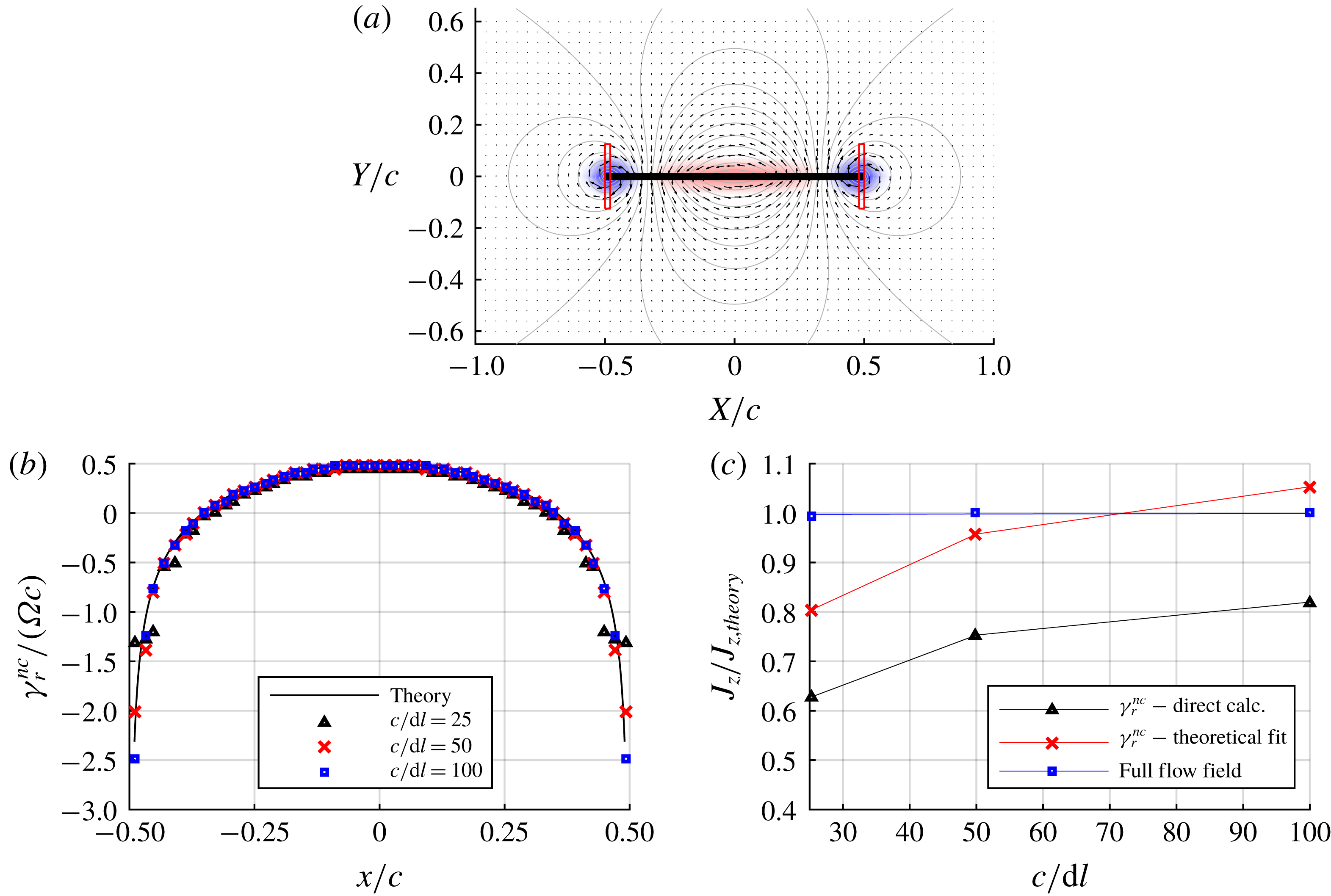
Quantification of discretisation errors using an artificially generated flow field for the rotating plate case. (a) Artificial flow field for $c/\unicode[STIX]{x0394}l=25$ . Shaded areas show the vorticity field, contours show the potential flow streamfunction while the rectangles at each plate edge show the first and last contours for the calculation of bound circulation. (b) The measured non-circulatory vortex sheet compared with potential theory. (c) Ratio of the measured to theoretical first moment of impulse. In panel (c): blue squares, first moment of impulse calculated from vorticity in the full flow field; black triangles, non-circulatory vortex sheet as directly measured; red crosses, analytical function fitted to the measured non-circulatory vortex sheet.

The flow field for the grid resolution of 25 vectors per chord is shown in figure 15(a). The red boxes are the first and last integration contours used for the calculation of bound circulation, the shaded background indicates vorticity calculated using the low-resolution vector field with the method described in § 5.1, and the contours show the potential flow streamfunction. The averaging process spreads vorticity past the left and right boundaries of the integration contours; thus some of the vorticity will be falsely allocated as ‘free’ in the flow field. Measurements of the non-circulatory bound vortex sheet, $\unicode[STIX]{x1D6FE}_{r}^{nc}$ , for each grid resolution are given in figure 15(b). Each measure of the bound vortex sheet approximately follows the theoretical value, albeit the lower resolutions show significant deviation from theory at the plate edges where there are large gradients in vorticity.

The first moment of impulse, $J_{z}$ , was calculated in three ways. One method uses all vorticity in the flow field, as determined from the secondary vector field. In discretised form, the second moment of vorticity given by (A 14) is

(B 1)

$$\begin{eqnarray}\unicode[STIX]{x1D6FD}_{z}=\mathop{\sum }_{k=1}^{n}(x_{k}^{2}+y_{k}^{2})\unicode[STIX]{x1D714}_{k}(\unicode[STIX]{x0394}l)^{2},\end{eqnarray}$$

where the subscript $k$ is the index for each vortex element in the discretised flow field. With (A 16), $J_{z}$ can therefore be found from the measured vorticity elements. This is the line identified by blue square markers shown in figure 15(c), scaled by the theoretical potential flow value given by (A 16). Despite the significant smoothing of vorticity around the plate surface, the resolution of the secondary grid has negligible effect on the first moment of impulse. Given reasonable vector resolution, the result suggests that, if vector elements contained by an arbitrary body are prescribed velocities equal to the rigid-body kinematics, subsequent calculation of vorticity from the velocity field will result in surface vortex sheets being represented in a spatially averaged form in the discretised vector field. Impulse and force quantities derived from such a discretised flow field will therefore include added-mass effects.

The problem with directly calculating impulse (and moments thereof) from flow field vorticity is that the added-mass contribution is superimposed with other vorticity sources. To isolate the added-mass component, impulse is calculated from the measure of $\unicode[STIX]{x1D6FE}^{nc}$ acquired from the procedure outlined in § 2.3. For the rotation case, this is given by the line identified by black triangles in figure 15(c). The significant error may in part be attributed to relatively high measurement error at the plate edges.

Figure 16.

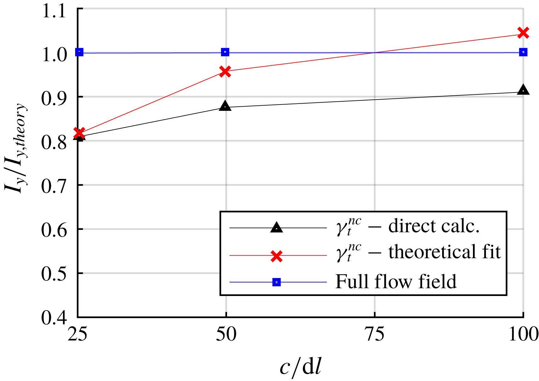
Ratio of measured to theoretical impulse for the translation case. Blue square markers – impulse derived from elemental vorticity over the entire flow field. Black triangles – the non-circulatory vortex sheet as directly measured. Red crosses – analytical function fitted to the measured non-circulatory vortex sheet.

For the purpose of extracting the portion of the impulse (and moments thereof) attributed to the non-circulatory vortex sheet, it is proposed that some of the discretisation error may be corrected by fitting the analytical non-circulatory vortex sheet function given by (2.4) to the measurements. For each kinematic case, rotation or translation, the analytical function is a geometrical ‘mode shape’ that is scaled by the instantaneous velocity. Provided the measures of the non-circulatory vortex sheet follow the geometric shape (this was demonstrated in § 5.3), a measure of the plate kinematics $U_{n}$ or $\unicode[STIX]{x1D6FA}$ may be obtained by using a least-squares fit or similar. Then impulse and force may be directly calculated from the analytical solutions given in appendix A. This is the line identified by red cross markers in figure 15(c). For the lowest vector resolution case, the error is halved to 20 %, whereas it is within $\pm 5\,\%$ for $c/\unicode[STIX]{x0394}l=50$ and 100. Each of the impulse measures for the translation case are given in figure 16. Once again errors are negligible when impulse is calculated using all elemental vorticity. The error is approximately half that of the rotation case for impulse calculated from the measured non-circulatory vortex sheet, and is comparable to the rotation case for the fitted vortex sheet.

B.2 PIV vector element error

The measurement error for each PIV vector point was estimated based on the work of Raffel et al. (Reference Raffel, Willert, Wereley and Kompenhans2007) and Nobach & Bodenschatz (Reference Nobach and Bodenschatz2009), who quantified error sources through simulations with synthetically generated particles. The error (in pixels) for each cross-correlated interrogation window may be expressed as

(B 2)

$$\begin{eqnarray}\sum \unicode[STIX]{x1D716}_{PIV}=\unicode[STIX]{x1D716}_{bias}+\unicode[STIX]{x1D716}_{rms_{0}}+\unicode[STIX]{x1D716}_{rms_{\unicode[STIX]{x1D6FF}}}+\unicode[STIX]{x1D716}_{rms_{\unicode[STIX]{x1D70C}}}+\unicode[STIX]{x1D716}_{rms_{i}}.\end{eqnarray}$$

The root-mean-square (r.m.s.) error $\unicode[STIX]{x1D716}_{rms_{0}}$ is due to random variation in particle image diameter, $\unicode[STIX]{x1D716}_{rms_{\unicode[STIX]{x1D6FF}}}$ is attributed to image displacement, $\unicode[STIX]{x1D716}_{rms_{\unicode[STIX]{x1D70C}}}$ results from particle density in each interrogation window and $\unicode[STIX]{x1D716}_{rms_{i}}$ from variation in particle intensity due to particle motion in the direction perpendicular to the laser plane. The consistent bias error $\unicode[STIX]{x1D716}_{bias}$ is attributed to in-plane loss of particle pairs. An estimate for each parameter is given in table 3. The peak particle displacement for the surge and rotation cases is approximately 4 and 6 pixels, respectively. With a total random error of 0.145 pixel, for each case the random error for an individual test run is 3.6 % and 2.4 %. Following batch averaging, the sum of random errors reduce to 1.6 % and 1.1 % as random error scales with $1/\sqrt{N}$ , where $N$ is the number of samples (Adrian & Westerweel Reference Adrian and Westerweel2011). The bias errors are 0.25 % and 0.16 % for the surge and rotation cases, respectively. The total error in velocity is estimated to be less than 2 % for both the rotation and surge test cases.

Table 3.

Contributions to PIV data error (pixels). Estimated from Raffel et al. (Reference Raffel, Willert, Wereley and Kompenhans2007) and Nobach & Bodenschatz (Reference Nobach and Bodenschatz2009).

References

Adrian, R. J. & Westerweel, J. 2011 Particle Image Velocimetry. Cambridge University Press.Google Scholar

Benjamin, T. B. 1986 Note on added mass and drift. J. Fluid Mech. 169, 251–256.Google Scholar

Brennen, C. E.1982 A review of added mass and fluid inertial forces. Tech. Rep. CR 82.010. Naval Civil Engineering Laboratory.Google Scholar

Buchner, A. J., Buchmann, N., Kilany, K., Atkinson, C. & Soria, J. 2012 Stereoscopic and tomographic PIV of a pitching plate. Exp. Fluids 52 (2), 299–314.Google Scholar

Corkery, S. J., Babinsky, H. & Harvey, J. K. 2018 On the development and early observations from a towing tank-based transverse wing–gust encounter test rig. Exp. Fluids 59 (9), 135.Google Scholar

Darwin, C. 1953 Note on hydrodynamics. Math. Proc. Cambridge Philos. Soc. 49 (2), 342–354.Google Scholar

Eldredge, J. D. 2010 A reconciliation of viscous and inviscid approaches to computing locomotion of deforming bodies. Exp. Mech. 50 (9), 1349–1353.Google Scholar

Graham, W. R., Pitt Ford, C. W. & Babinsky, H. 2017 An impulse-based approach to estimating forces in unsteady flow. J. Fluid Mech. 815, 60–76.Google Scholar

Lamb, H. 1895 Hydrodynamics. Cambridge University Press.Google Scholar

Leonard, A. & Roshko, A. 2001 Aspects of flow-induced vibration. J. Fluids Struct. 15 (3–4), 415–425.Google Scholar

Milne-Thomson, L. M. 1986 Theoretical Hydrodynamics, 5th edn. Macmillan.Google Scholar

Nobach, H. & Bodenschatz, E. 2009 Limitations of accuracy in PIV due to individual variations of particle image intensities. Exp. Fluids 47 (1), 27–38.Google Scholar

Pitt Ford, C. W. & Babinsky, H. 2013 Lift and the leading-edge vortex. J. Fluid Mech. 720, 280–313.Google Scholar

Poelma, C., Dickson, W. B. & Dickinson, M. H. 2006 Time-resolved reconstruction of the full velocity field around a dynamically-scaled flapping wing. Exp. Fluids 41 (2), 213–225.Google Scholar

Polet, D. T., Rival, D. E. & Weymouth, G. D. 2015 Unsteady dynamics of rapid perching manoeuvres. J. Fluid Mech. 767, 323–341.Google Scholar

Raffel, M., Willert, C. E., Wereley, S. T. & Kompenhans, J. 2007 Particle Image Velocimetry: A Practical Guide, 2nd edn. Springer.Google Scholar

Rival, D. E., Prangemeier, T. & Tropea, C. 2009 The influence of airfoil kinematics on the formation of leading-edge vortices in bio-inspired flight. Exp. Fluids 46 (5), 823–833.Google Scholar

Saffman, P. G. 1992 Vortex Dynamics. Cambridge University Press.Google Scholar

Stevens, P. R. R. J. & Babinsky, H. 2017 Experiments to investigate lift production mechanisms on pitching flat plates. Exp. Fluids 58 (1), 7.Google Scholar

Wu, J. C. 1981 Theory for aerodynamic force and moment in viscous flows. AIAA J. 19 (4), 432–441.Google Scholar

Figure 1.Streamlines for a flat plate with chord length $c$ in potential flow: (a) translation with velocity $U_{n}$; (b) rotation with angular velocity $\unicode[STIX]{x1D6FA}$ about the mid-chord. Streamlines are shown for the moving-body reference frame.

Figure 2.Schematic comparing vorticity distributions between potential flow (a) and a viscous flow field (b). In the viscous fluid, vorticity is diffused and advected from the plate surface, whereas vorticity is contained in an infinitely thin layer for the inviscid fluid. Red and blue colours correspond to positive and negative vorticity, respectively.

Figure 3.Problem geometry and coordinates frames: (a) global ‘fixed’ coordinate frame and (b) plate frame.

Figure 4.Representation of the plate as a vortex sheet $\unicode[STIX]{x1D6FE}(x)$, given by the difference in surface slip velocities $u_{1}(x)$ and $u_{2}(x)$.

Figure 5.Schematic of a vortex element with circulation $\unicode[STIX]{x1D6E4}_{k}$ in the mapped circle frame, showing the corresponding ‘mirror’ with circulation $-\unicode[STIX]{x1D6E4}_{k}$.

Figure 6.Elements used for the calculation of the boundary layer circulation: (a) overview showing integration contour elements distributed across the plate chord; (b) schematic showing a single integration element encompassing boundary layers.

Figure 7.Schematic of towing tank, PIV and flow visualisation configurations: (a) end view; (b) top view showing the laser overlap plane and camera set-up. Adapted from Stevens & Babinsky (2017).

Table 1.Surging plate kinematics.

Table 2.Rotating plate kinematics.

Figure 8.Dye flow visualisation (a–c) and PIV flow field measurements (d–f) for the surge test case: (a,d) $X_{c}/c=-0.02$; (b,e) $X_{c}/c=-1.00$; (c,f) $X_{c}/c=-1.98$. Only every fourth velocity vector is shown; $Re=10\,000$.

Figure 9.Dye flow visualisation (a–c) and PIV flow field measurements (d–f) for the rotating plate case: (a,d) $\unicode[STIX]{x1D6FD}\approx 1^{\circ }$; (b,e) $\unicode[STIX]{x1D6FD}=90^{\circ }$; (c,f) $\unicode[STIX]{x1D6FD}=180^{\circ }$. Only every fourth velocity vector is shown. $Re=4600$.

Figure 10.Sums of the boundary layer and bulk flow circulation elements: (a) surge case; (b) rotation case.

Figure 11.Comparison of measured and potential flow vortex sheets between potential theory and experiment for the surge (a) and rotation (b) cases.

Figure 12.PIV data of the flow field at $\unicode[STIX]{x1D6FD}=180^{\circ }$: (a) before the deceleration impulse, $\unicode[STIX]{x1D6FD}=180^{\circ -}$; (b) after the impulse, $\unicode[STIX]{x1D6FD}=180^{\circ +}$; (c) the change to the flow field for the rotation test case; (d) the change to the bound vortex sheet across the deceleration impulse compared with potential theory. Only every fourth PIV vector is shown.

Figure 13.Surge case: (a) impulse compared between potential theory, the experimentally measured full flow field and the measured non-circulatory bound vortex sheet; (b) comparison of the added-mass attributed drag force coefficient between theory and the measured non-circulatory bound vortex sheet. For clarity, drag force coefficients are filtered using a bidirectional moving window average with a window period of 0.15 s.

Figure 14.Rotation case: (a) first moment of impulse compared between potential theory, the experimentally measured full flow field and the measured non-circulatory bound vortex sheet; (b) comparison of the added-mass attributed pitching moment between theory and the measured non-circulatory bound vortex sheet. No filtering is employed.

Figure 15.Quantification of discretisation errors using an artificially generated flow field for the rotating plate case. (a) Artificial flow field for $c/\unicode[STIX]{x0394}l=25$. Shaded areas show the vorticity field, contours show the potential flow streamfunction while the rectangles at each plate edge show the first and last contours for the calculation of bound circulation. (b) The measured non-circulatory vortex sheet compared with potential theory. (c) Ratio of the measured to theoretical first moment of impulse. In panel (c): blue squares, first moment of impulse calculated from vorticity in the full flow field; black triangles, non-circulatory vortex sheet as directly measured; red crosses, analytical function fitted to the measured non-circulatory vortex sheet.

Figure 16.Ratio of measured to theoretical impulse for the translation case. Blue square markers – impulse derived from elemental vorticity over the entire flow field. Black triangles – the non-circulatory vortex sheet as directly measured. Red crosses – analytical function fitted to the measured non-circulatory vortex sheet.

Table 3.Contributions to PIV data error (pixels). Estimated from Raffel et al. (2007) and Nobach & Bodenschatz (2009).

Article contents

Quantification of added-mass effects using particle image velocimetry data for a translating and rotating flat plate

Abstract

JFM classification

Information

1 Introduction

2 Theoretical description of the vortex sheets

2.1 Problem geometry

2.2 Vortex sheet

2.2.1 Non-circulatory ‘added-mass’ vortex sheet

2.2.2 Circulatory ‘shed vorticity’ vortex sheet

2.3 Potential flow model summary

3 Quantification of $\unicode[STIX]{x1D6FE}^{b}$ from particle image velocimetry

4 Description of the experiments

4.1 PIV and flow visualisation

4.2 Plate kinematics

5 Results

5.1 Flow topology

5.2 Single-sided flow field circulation

5.3 Non-circulatory vortex sheets

5.4 Instantaneous non-circulatory vortex sheet

5.5 Impulse and forces from PIV

6 Lost circulation compensation

7 Conclusion

Acknowledgements

Appendix A.

A.1 General solution

A.2 Surface velocity and bound vortex sheet

A.3 Linear impulse and force

A.4 First moment of impulse and mid-chord moment

Appendix B.

B.1 Vortex sheet discretisation error

B.2 PIV vector element error

References

Save article to Kindle

Save article to Dropbox

Save article to Google Drive

Reply to: Submit a response

Your details

You have entered the maximum number of contributors

Conflicting interests